Saving Money for Analytical Workloads in the Cloud

Abstract.

As users migrate their analytical workloads to cloud databases, it is becoming just as important to reduce monetary costs as it is to optimize query runtime. In the cloud, a query is billed based on either its compute time or the amount of data it processes. We observe that analytical queries are either compute- or IO-bound and each query type executes cheaper in a different pricing model. We exploit this opportunity and propose methods to build cheaper execution plans across pricing models that complete within user-defined runtime constraints. We implement these methods and produce execution plans spanning multiple pricing models that reduce the monetary cost for workloads by as much as 56%. We reduce individual query costs by as much as 90%. The prices chosen by cloud vendors for cloud services also impact savings opportunities. To study this effect, we simulate our proposed methods with different cloud prices and observe that multi-cloud savings are robust to changes in cloud vendor prices. These results indicate the massive opportunity to save money by executing workloads across multiple pricing models.

1. Introduction

As analytic workloads migrate to cloud data warehouses, users care just as much about saving money as they do about optimizing workload runtime. Even modest savings on one workload become significant over time if the workload runs repeatedly. For example, saving $140 on an analytics workload that runs twice a day to update recommendations will save $100,000 a year, and organizations may have many such workloads that power different applications such as filling dashboards to visualize complex data patterns or managing ETL pipelines (What is OLAP?, [n.d.]; Tejada, [n.d.]; Snowflake ETL, [n.d.]; Goff, [n.d.]; Martinez, 2021; Google ETL, [n.d.]; Dashboard, [n.d.]).

While cloud providers offer many tools to tune database performance, there are no mechanisms to directly save money. Thus, users are increasingly employing setup-specific solutions to save costs such as working with consulting groups like McKinsey, the DuckBill group, or CloudZero (The Duckbill Group, [n.d.]; CloudZero, [n.d.]; McKinsey, [n.d.]) to tune databases, turn off unused resources, and optimally utilize allocated resources.

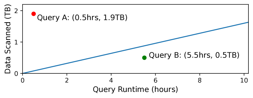
Figure 1. Size scanned (TB) vs. runtime (hours). Boundary for $6.25/TB (pay-per-byte) vs. $1/hour (pay-per-compute).

A blue line with slope of 0.16 separates a red point labelled Query A at coordinates (0.5 hours run, 1.9TB scanned) and a green point labelled Query B at coordinates (5.5 hours run, 0.5 TB scanned).

In this paper, we identify opportunities to reduce the monetary cost of running analytical workloads in the cloud. The key insight is simple. Queries consume IO and CPU; but cloud databases’ pricing models charge for IO or CPU time, to keep pricing simple. This opens an opportunity to save money by cleverly scheduling queries in a cloud database with a favorable pricing model.

The two most prominent pricing models for cloud databases are pay-per-compute and pay-per-byte. In a pay-per-compute model the user pays for computation time, e.g., in AWS Redshift (Armenatzoglou et al., 2022), while in pay-per-byte the user pays for the amount of data scanned irrespective of compute time, e.g., in Google BigQuery (BigQuery, [n.d.]).

CPU-bound queries execute cheaper in pay-per-byte models, vice versa for IO-bound queries. Figure 1 plots query runtime (hours) on the $x$ axis and the amount of data scanned (terabytes) on the $y$ axis. We consider one cloud database charging $6.25/TB (pay-per-byte) and one charging $1/hour (pay-per-compute). Queries on the blue line cost the same in both databases, e.g. one that runs for 6.25 hours and scans 1TB. Query A runs fast but reads 1.9TB (e.g., a simple scan query). It costs less in the pay-per-compute database, so it is above the line. Query B scans 0.5TB but runs slower (e.g., window operations), so it costs less in the pay-per-byte database. Running each query in the pricing model most beneficial for it is cheaper than running both queries in a single cloud database.

All workloads have runtime constraints, even if they are loose. For example, a user with a nightly workload that usually finishes by 2 am may prefer to delay the completion time up to 8am if they can save money (BigQuery Reliability, [n.d.]). This distills the problem we explore in this paper: given an analytical workload (a set of queries and data) and a workload runtime constraint, we propose two algorithms to exploit money saving opportunities that arise from the observations above:

• O1: Inter-Query Algorithm. We propose an algorithm that takes a set of queries, data, a workload runtime constraint, and a set of cloud databases and identifies which queries should execute in which databases to save money within the runtime constraint.

• O2: Intra-Query Algorithm. We propose an algorithm that, given a single query, a query runtime constraint, and a set of target cloud databases finds subqueries to execute in each cloud database to reduce query cost within the runtime constraint.

Where these complementary techniques are best applied is workload dependent, e.g., a workload with 3 expensive queries may benefit more from O2 than O1, so we consider each in isolation. However, both O1 and O2 require moving data, ensuring cloud database SQL syntax compatibility, and, more importantly, managing the costs of data movement. To exploit O1 and O2 without modifying user setups, we implement middleware called Arachne between users and the cloud that takes a workload and runtime constraint, executes O1–O2, migrates data, and yields cheaper execution plans when these exist under the runtime constraint.

We use Arachne to study the impact of O1–O2 on workload costs under runtime constraints. We build execution plans across Amazon Redshift (pay-per-compute) (Armenatzoglou et al., 2022) and Google BigQuery (pay-per-byte) (BigQuery, [n.d.]) to evaluate Arachne, and we carefully configure these systems to the best of our ability (Scaer et al., 2020; Burman et al., 2022; BigQuery Optimizing, [n.d.]; Sharma and Fu, [n.d.]).

Our results show that there are massive opportunities for saving money. We achieve up to 57% savings (we run workloads for $104 while the original cost $243) with an inter-query plan across pricing models that has a nearly 10 hour slowdown. On another workload, an inter-query plan saves 55% with a 3-hour speedup. We also achieve up to 90% savings on a query via an intra-query plan.

We simulate varying cloud prices and study multi-cloud savings and runtime-cost tradeoffs as prices change. We see that savings are robust to price changes and that varying egress fees–what cloud vendors charge to move data out of a cloud–can aid or fully prevent data movement. In summary, the contributions of this paper are:

• We observe cost saving opportunities for analytical workloads by exploiting different cloud pricing models.

• We design two algorithms to exploit those opportunities.

• We implement the algorithms on a system called Arachne, to realize savings for real workloads.

• We evaluate Arachne (and the algorithms it implements) using prominent cloud databases and provide a simulation to shed light on the impact of market prices on saving opportunities.

Next, Section 2 presents background and the cost saving opportunity. Sections 3 and 4 present the inter- and intra-query algorithms to exploit O1 and O2, and Section 5 presents Arachne. We evaluate savings opportunities in Section 6 and present related work in Section 7 and conclusions in Section 8.

2. Background and Opportunities

We provide background on analytical workloads in the cloud in Section 2.1, characterize the savings opportunity in Section 2.2, and present the problem statement in Section 2.3.

2.1. Executing Analytics Workloads in the Cloud

2.1.1. Cloud Data Warehouses and Pricing Models

We differentiate infrastructure-as-a-service (IaaS) from platform-as-a-service (PaaS) and within PaaS, we separate pay-per-compute from pay-per-byte.

IaaS vs PaaS. In IaaS, OLAP databases (e.g., Trino (Sethi et al., 2019) or Apache Hive (Thusoo et al., 2010a)) are manually deployed and maintained on virtual machines and billed by compute time. In contrast, PaaS (e.g., Google BigQuery (BigQuery, [n.d.]), AWS Redshift (Armenatzoglou et al., 2022), Microsoft Azure Synapse (Azure Synapse, [n.d.]), or Snowflake (Dageville et al., 2016)) deploy and maintain databases for users to directly use. PaaS charges more than IaaS for these services.

Pay-per-compute vs Pay-per-byte. Two of the most common PaaS pricing models are pay-per-compute, which charges for the amount and duration of computing resources, and pay-per-byte, which charges for the bytes read by a query regardless of runtime.

Table 1. Prices for pay-per-compute (PPC), pay-per-byte (PPB), storage, and egress. Systems in evaluation are bolded.

Pricing Model	Database	Cost
PPC	Amazon Redshift–ra3.xlplus	$1.086/hr
PPC	Amazon Redshift–ra3.4xlarge	$3.26/hr
PPC	Azure Synapse 100 DWU	$1.20/hr
PPC	Azure Synapse 500 DWU	$6/hr
PPC	Snowflake Small (AWS US-East)	$4/hr
PPC	n2-standard-32 VM (GCP)	$1.55/hr
PPC/PPB	Amazon Redshift Spectrum	RS + $5/TB
PPB	Google BigQuery	$6.25/TB
PPB	Amazon Athena	$5/TB
PPB	Azure Synapse Serverless	$5/TB

Cloud Vendor	Storage	Writes	Reads	Egress
GCP (us-east1)	$0.023/GB-mo	$0.05/10k ops	$0.004/10k ops	$120/TB
S3 (us-east)	$0.023/GB-mo	$0.05/10k ops	$0.004/10k ops	$90/TB
Azure	$0.018/GB-mo	$0.065/10k ops	$0.005/10k ops	$87/TB

2.1.2. Breakdown of Cloud Costs

Loading data into a cloud database and executing a workload incurs the following costs:

• Blob Storage cost: Most cloud databases access data from blob storage (e.g., AWS S3), and storing data there has a cost (see Table 1). In S3 (us-east) it costs $23/month to store 1TB of data.

• Read/Write cost: Blob storage systems charge for API calls, e.g., read/write calls to store and retrieve data from blob storage. For instance, it costs $0.05 to perform 10,000 write operations in S3.

• Loading cost: While data is loaded into a machine, such a machine must be operative and thus consuming compute resources.

• Egress cost: Transferring data out of a cloud or between regions incurs per-byte charges. A 1TB transfer from GCP costs $120.

• Query Processing cost: Query execution can be billed per-byte or per-compute. BigQuery charges $6.25/TB scanned.

Running an analytics workload in the cloud involves four steps. In Step 1, data is collected from sources (e.g., on-premise repositories, sensors) and moved to the cloud, incurring data transfer and storage costs. In Step 2, data is loaded into a cloud database incurring read/write and loading costs. Moving data between clouds exacerbates these costs, so our algorithms account for this potential cost increase. In Step 3, users pay to execute queries against the data in the cloud database. Finally, in Step 4 query results are returned to users to use in downstream tasks, e.g., reporting, filling dashboards (BigQuery analytics, [n.d.]; Datta, 2022), potentially incurring egress costs. While all four steps incur costs, costs for Steps 1 and 4 depend on the input and output data, which are mostly fixed for a given workload. We concentrate on Steps 2 and 3 which involve cloud databases and dominate the total cost. We specifically focus on reducing the cost of Step 3 and, to the extent that data movement is needed, Step 2.

2.2. Cost Saving Opportunity and Challenges

We now exploit the insight that migrating CPU- or IO-bound queries or subqueries to an analytical system with a beneficial pricing model presents an cost saving opportunity.

Given the size scanned by a query ($S$), query runtime ($R$), per-byte cost ($\alpha_{S}$), and per-compute cost ($\alpha_{R}$), we observe that $\alpha_{S}\times S=\alpha_{R}\times R\implies S=\frac{\alpha_{R}}{\alpha_{S}}\times R$. So a query that runs for $R$ seconds costs the same in pay-per-compute as one that reads $\frac{\alpha_{R}}{\alpha_{S}}\times R$ bytes in pay-per-byte. This equation represents the blue line in Figure 1 that delineates the most beneficial pricing model for a query.

Arachne needs query runtimes to exploit savings opportunities within runtime constraints. Unfortunately, there are few accurate approaches to estimating query runtime ($R$) Instead, Arachne collects query runtime via a profiling stage described in Section 5.2.

Adapting to Cloud Vendor Pricing. This analysis only requires query cost and runtime, so Arachne can support other pricing models. For tiered pricing models–such as egress where in AWS the first 10TB/month cost $90/TB and the next 40TB/month cost $85/TB–Arachne can track usage and adjust pricing constants accordingly.

Arachne must also track cloud price changes to keep its analysis accurate, as users do today. However, pricing changes happen rarely and are announced well in advance. Google announced a recent BigQuery price increase 3 months in advance (BigQuery Pricing Change, [n.d.]) while Redshift pricing for current generation hardware has not changed for years.

2.3. Problem Statement and Approach

We now formally present the goal of this work. Given a workload of queries $Q$ and tables $T$ that execute on a source execution backend $X_{s}$ under a runtime constraint, we consider a set of execution backends (each of which may offer a different pricing model) and find inter- and intra-query plans (O1–O2) that save money within the runtime constraint. Users choose which algorithms to run on their workload, as O1 and O2 do not need to be deployed together.

Approach. To solve the problem statement, we build a proof-of-concept, Arachne, which implements the inter- and intra-query algorithms and shows empirically that it is possible to save money on analytical workloads by scheduling queries and subqueries across clouds. Arachne does not require modifications to existing setups, e.g., where data is stored, and it handles all needed data movement. Arachne relies on an offline profiling stage to gather query plans, runtimes, and costs to save money and meet runtime constraints.

We note that these algorithms can only honor runtime constraints up to the accuracy of the profiles, e.g., if cloud databases dramatically vary a query’s runtime between iterations, the algorithms cannot compute accurate runtime or cost estimates for plans. We discuss this further with profiling in Section 5.2.

3. Inter-Query Execution Plan

We now present the inter-query algorithm to exploit O1. We discuss the setup (Section 3.1) and algorithm intuition (Section 3.2.1), present the algorithm (Section 3.2.2), and compare it to an optimal inter-query algorithm (Section 3.2.3) to understand its quality.

3.1. Algorithmic Setup and Goal

We consider an analytics workload with a set of tables $T$, queries $Q$, and a workload runtime constraint. We assume that initially a user employs a source execution backend $X_{s}$, paying storage costs for $T$ in $X_{s}$, and paying execution costs for $Q$ in $X_{s}$.

Given a second execution backend, $X_{d}$, the algorithm chooses a subset of queries $W\subseteq Q$ to execute in $X_{d}$ such that the overall workload costs are reduced without breaking the runtime constraint. To run a query in $X_{d}$, all tables that the query scans must migrate from $X_{s}$ to $X_{d}$, so the algorithm must account for migration costs. The algorithm requires the following inputs:

• The set of tables $T$ and queries $Q$ in the workload.

• $DEADLINE$ is an optional workload runtime constraint.

• The source $X_{s}$ and destination $X_{d}$ execution backends e.g., AWS Redshift or Google BigQuery.

• A set of cloud prices P = $(p_{blob},p_{read},p_{write},p_{sec},p_{byte}$). $p_{blob}$ per-byte for blob storage, $p_{read}$ read and $p_{write}$ write cost, and execution backend costs $p_{sec}$ for per-compute pricing models and $p_{byte}$ for per-byte pricing models (example prices in Table 1)

• The egress cost $e$ to move from $X_{s}$ to $X_{d}$ e.g., $90/TB out of AWS.

• A function $s$ which returns the size of a given table. This is measured via cloud storage APIs and is defined for the sake of notation.

• Functions $C_{X_{i}}$ and $R_{X_{i}}$ which take a query $q$ and return the cost and runtime respectively of $q$ in an execution backend $X_{i}$.

All the above inputs are easy to obtain except for $C_{X_{i}}$ and $R_{X_{i}}$, which are obtained during a profiling stage, explained in Section 5. We now formalize the algorithm’s goal.

Considering the Problem as a Bipartite Graph. We construct a bipartite graph $G=(T,Q,E)$, with tables $T$ and queries $Q$. We draw an edge $(t\in T,q\in Q)\in E$ if query $q$ scans base table $t$.

We next assign weights $\sigma_{q}$ to each query $q\in Q$ and $\mu_{t}$ for each table $t\in T$. $\sigma_{q}$ represents the query savings achieved by moving query $q$ to the other execution backend, i.e.,

(1) $$\sigma_{q}=C_{X_{d}}(q)-C_{X_{s}}(q)$$

$\mu_{t}$ represents the migration costs for a table, which is the cost of moving $t$ from $X_{s}$ to $X_{d}$, loading $t$ into $X_{d}$, reading and writing $t$ from blob storage, and temporarily storing $t$ in blob storage. If each table requires $K$ read/write operations, we can express $\mu_{t}$ as:

(2) $$\mu_{t}=e\times s(t)+(p_{read}+p_{write})\times(s(t)/K)+p_{blob}\times s(t)$$

In Figure 2 we show an example of this model with three tables $T=\{t_{1},t_{2},t_{3}\}$ and three queries $Q=\{q_{1},q_{2},q_{3}\}$. We draw edges to represent query dependencies e.g., $q_{3}$ scans tables $t_{2},t_{3}$.

The algorithm’s goal is to find a subset of tables that maximizes query savings. Concretely, for $S\subseteq T$ let $N(S)$ be the set of queries scanning tables in $S$ and let $N^{-1}(q\in Q)$ be the set of tables $q$ scans. Our goal is to find $S_{\theta}$ in Equation 3. For example, in Figure 2 we move tables $t_{2},t_{3}$ and queries $q_{2},q_{3}$ to $X_{d}$, saving (3+4)-(2+4)=$1.

(3) $$S_{\theta}=\operatorname*{arg\,max}_{S\subset T}\sum\limits_{q\in N(S)}{\sigma_{q}}-\sum\limits_{s\in S}{\mu_{s}}$$

3.2. Inter-Query Algorithm

Now we provide the intuition for our greedy strategy to exploit O1 (Section 3.2.1), and present the inter-query algorithm (Section 3.2.2). Finally, we assess the quality of the greedy algorithm by comparing it to an optimal (but much slower) min-cut algorithm (Section 3.2.3).

3.2.1. Intuition for the Greedy Strategy

At each iteration, the greedy algorithm computes the maximum savings achievable (upper bound) by moving queries depending on $t$ to $X_{d}$ for each table $t$. It removes the table with the least upper bound and records the cost and runtime of the resulting inter-query plan. When no tables remain, it chooses the cheapest plan with runtime under the runtime bound.

Concretely, we define $v_{t}=(\sum_{q\in N(t)}{\sigma_{q}})-\mu_{t}$ as the sum of query savings for all queries that scan $t$ minus the migration cost of $t$. As an upper bound on savings, if $v_{t}<0$ it will never be beneficial to move $t$ to the destination backend, so we remove nodes for $t$ and all queries scanning $t$ from the bipartite graph.

Analogously, we define a lower bound on savings generated from a single query, $v_{q}$, as query savings of $q$ minus the migration costs of the tables that $q$ requires, or $v_{q}=\sigma_{q}-\sum_{t\in N^{-1}(q)}{\mu_{t}}$. As a lower bound on possible savings for $q$, if $v_{q}>0$ it is strictly beneficial to move $q$ to $X_{d}$. To represent this we add $q$ and $N^{-1}(q)$ to the final set of queries and tables to move to $X_{d}$, we remove the nodes representing $q$ and all $t\in N^{-1}(q)$ from the bipartite graph, and remove all outbound edges from $N^{-1}(q)$. In Figure 2 we compute $v_{t}$ and $v_{q}$ and present them in the lower half of each node, e.g., $v_{t_{2}}$ is the savings of $q_{1}$ and $q_{3}$ minus the cost of $t_{2}$, or $3+4-2=5$.

Algorithm Example. In Figure 3 the algorithm considers three plans for the given workload. The first plan (left) migrates all tables and queries, saving $65 but violating the runtime constraint, so runtime is colored red. Removing $t_{3}$ yields the second plan (middle), saving $40 and running in 2.5 hours, so both savings and runtime are colored green. Finally, removing $t_{1}$ yields the baseline (right) which saves no money. The second plan is chosen as it saves the most money under the runtime constraint, so it is colored green.

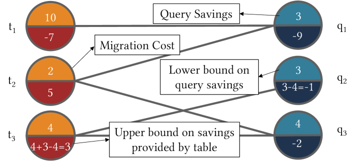
Figure 2. Bipartite model. Node top is query savings $\sigma_{q}$ or migration cost $\mu_{t}$. Node bottom is upper bound $v_{t}$ or lower bound $v_{q}$. We show how this value is calculated for ${t_{3}}$ and ${q_{2}}$.

Bipartite graph. Left side has three circles labelled t1, t2, and t3. The top half is colored orange and the bottom half is red. Each half contains a number. Labels indicate that for the left circles, the top half indicates migration cost while the bottom indicates the upper bound on savings provided by the table. The right side has three circles labelled q1, q2, and q3. The top of these is a lighter blue and the bottom is a darker blue. Labels indicates that the top number is query savings and the bottom is the lower bound on query savings. Lines connect left circles to those on the right. The top of t3 has a 4. t3 is connected to q2 and q3. The top of q2 has a 3, the top of q3 has a 4. The bottom half of t3 contains an equation, 4+3-4=3. This adds the tops of q2 and q3 and subtracts the top of t3. An analogous equation is shown on the bottom of q2 which is only connected to t3. This equation shows 3-4=-1. This adds the top of q2 and subtracts the top of t3.

1 Function InterQuery($\{X_{s},X_{d}\}$, prices P, $e$, $T$, $Q$, $s$, $C$, $R$, $DEADLINE$):

2       $T^{\prime},Q^{\prime},T_{f},Q_{f}$ = ReducePlan(X, P, e, T, Q, s, C) ;

3       Remove all outbound edges from $T_{f}$ ;

4      

5      while  $T^{\prime}\neq\emptyset$ do

6             For $t\in T^{\prime}$, $v_{t}=(\sum_{q\in N(t)}{\sigma_{q}})-\mu_{t}$ ;

7             $t^{\prime}\in T^{\prime}$ be the table with minimium $v_{t^{\prime}}$ ;

8             $T^{\prime}=T^{\prime}-\{t^{\prime}\}$; $Q^{\prime}=\{q|N^{-1}(q)\subset T^{\prime}\}$ ;

9             $T^{\prime},Q^{\prime},T_{f}^{\prime},Q_{f}^{\prime}=ReducePlan(X,e,T^{\prime},Q^{\prime},s,f)$ ;

10             $T^{\prime}=T^{\prime}\cup T_{f}^{\prime}$; $Q^{\prime}=Q^{\prime}\cup Q_{f}^{\prime}$ ;

11             planCosts[$T^{\prime},Q^{\prime}$] = $\langle$cost($T^{\prime},Q^{\prime}$), runtime($T^{\prime},Q^{\prime}$)$\rangle$ ;

12            

13      Return the min cost plan in planCosts within $DEADLINE$ ;

14      

15Function ReducePlan($X$, P, $e$, $T^{\prime}$, $Q^{\prime}$, $s$, $C$):

16       $Q^{\prime}=\{q|\sigma_{q}>0\}$ ; $T_{f},Q_{f}=\{\},\{\}$ ;

17      

18      For $t\in T^{\prime}$ $v_{t}=(\sum_{q\in N(t)}{\sigma_{q}})-\mu_{t}$ ;

19       For $q\in Q^{\prime}$ $v_{q}=\sigma_{q}-\sum_{t\in N^{-1}(q)}{\mu_{t}}$ ;

20      

21      while  $T^{\prime}\neq\emptyset\land\exists v_{t}<0\land\exists v_{q}>0$ do

22             $U=\{t|v_{t}<0\}$; $V=\{q|v_{q}>0\}$ ;

23             $T^{\prime}=T^{\prime}-U$ ; $Q^{\prime}=Q^{\prime}-\{q|q\in N(t)\forall t\in U\}$ ;

24             $T^{\prime}=T^{\prime}-\{t|t\in N^{-1}(q)\forall q\in V\}$ ; $Q^{\prime}=Q^{\prime}-V$ ;

25             $T_{f}=T_{f}\cup\{t|t\in N^{-1}(q)\forall q\in V\}$ ; $Q_{f}=Q_{f}\cup V$ ;

26             For $t\in T^{\prime}$ $v_{t}=(\sum_{q\in N(t)}{\sigma_{q}})-\mu_{t}$ ;

27             For $q\in Q^{\prime}$ $v_{q}=\sigma_{q}-\sum_{t\in N^{-1}(q)}{\mu_{t}}$ ;

28            

29      return $T^{\prime},Q^{\prime},T_{f},Q_{f}$;

30      

Algorithm 1 Inter-query greedy algorithm

3.2.2. The Inter-Query Algorithm in Depth

The greedy algorithm, shown in Algorithm 1, first invokes ReducePlan (line 2), which computes $v_{t}$ and $v_{q}$ (lines 14–15), removes tables with $v_{t}<0$ from consideration, and migrates queries with $v_{q}>0$ to $X_{d}$ (lines 17–22). This loop repeats until there are no more candidates or there are no tables left (line 16). ReducePlan returns the tables and queries to migrate and the remaining tables and queries to consider (line 23).

The algorithm then removes all outbound edges from the tables migrating to $X_{d}$ (line 3) and proceeds to greedily remove tables from consideration. While there are still tables (line 4), the algorithm computes $v_{t}$ (line 5), assigns $t$ with minimal $v_{t}$ to remain in $X_{s}$, and removes nodes in $N(t)$ (line 6–7). The algorithm calls ReducePlan again to prune away tables with $v_{t}<0$ and identify queries with positive lower bounds (line 8). The algorithm records the cost and runtime of the current plan using query costs and runtimes $C$ and $R$, cloud prices $P$, and table sizes $s$ (line 10).

Finally, the algorithm chooses the cheapest plan in $planCosts$ with runtime less than $DEADLINE$ (line 11). The baseline plan– migrating no tables or queries–will be cached in $planCosts$ and will be chosen if no cheaper plans exist under the runtime constraint.

3.2.3. Optimal Algorithm and Complexity Analysis

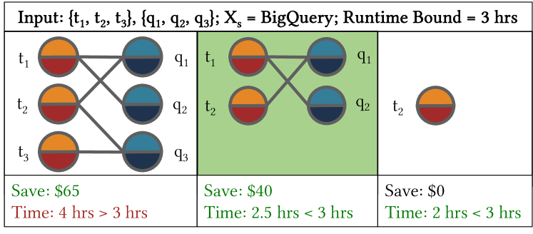
Figure 3. The plans considered with a 3 hour runtime bound. Plan B saves the most money within 3 hours so it is chosen.

A diagram showing the three plans considered for a problem with three tables as input labelled t1, t2, and t3 and three queries as input q1, q2, and q3. The starting cloud is BigQuery, and the runtime bound is 3 hours. The first plan considers migrating all tables and queries. This saves 65 dollars but runs in 4 hours, which is longer than the runtime bound. The second plan removes t3 and q3. This saves 40 dollars and runs in 2.5 hours, which is under the runtime bound. The final plan only contains t2. This saves 0 dollars and runs in 2 hours, the fastest of the three. The second plan is shaded green, as it saves the most money of the plans that run under 3 hours.

To evaluate the greedy algorithm we: i) present an optimal min-cut based inter-query algorithm; ii) compare its runtime complexity to the greedy approach; iii) and show the greedy algorithm’s accuracy in practice.

Optimal Solution. As in (Heller et al., 2021), we build a capacity function $c$ and a bipartite graph $G$ with tables on the left and queries on the right. Edges with infinite capacity connect tables and queries by query dependencies. We add a source node $a$ and draw edges from $a$ to every table $t_{i}$; $c((a,t_{i}))=\mu_{t_{i}}$. We add a sink node $b$ and draw edges from every query $q_{j}$ to $b$; $c((q_{j},b))=\sigma_{q_{j}}$. The algorithm finds the min-cut $(A,B)$ and migrates the queries and tables in $B$ to $X_{d}$.

Complexity Analysis. Using a min-cut algorithm (Edmonds and Karp, 1972; Dinitz, 2006), the optimal algorithm has complexity $O(|V|^{2}|E|)$. For the greedy approach, (note: $|V|=|T|+|Q|$), computing $v_{t}$ or $v_{q}$ is $O(|V|)$ with at worst $|T|$ iterations, yielding a worst-case complexity of $O(|T||V|)$. The optimal algorithm is both an order of magnitude less efficient and depends on the number of relationships between queries and tables. The greedy algorithm is independent of query complexity.

Practical Significance. This difference in complexity between the optimal and greedy algorithms has practical significance when the number of queries and tables is large. For example, when using the TPC-DS workload as input (24 tables and 100 queries), the difference is insignificant, with both algorithms running in less than 0.3 seconds. With 1000 queries and 100 tables, the optimal runtime jumps to 3.4 seconds, while the greedy remains under 0.3 seconds. With 2500 queries and 400 tables, the optimal algorithm takes 2.1 minutes while the greedy takes 1.2 seconds.

Greedy Algorithm Accuracy. To evaluate accuracy, we use 72 workloads at 1TB and 2TB, both with and without IaaS, and using both internal and external BigQuery storage, producing 576 workloads. We run the greedy and optimal algorithms on each workload. Our greedy strategy finds the optimal solution for all workloads.

4. Intra-Query Execution Plan

We now present the intra-query algorithm to exploit O2. We first present the setup (Section 4.1) and how to identify where to make cuts (Section 4.2) before presenting the algorithm (Section 4.3).

4.1. Algorithmic Setup and Goal

The setup is similar to that in Section 3.1, but this algorithm takes a single query $q$ and a runtime constraint for $q$ and finds a subquery that saves money when migrated from $X_{s}$ to $X_{d}$ after accounting for migration costs while honoring the runtime constraint.

Formalization and Goal. A query plan is a directed acyclic graph where leaves represent base tables and edges represent data flow from upstream tables to downstream operators. Removing all outbound edges from a node partitions the graph into two disjoint subgraphs; we call this process making a cut in the query plan at a node. The goal of the intra-query algorithm is to find a profitable cut of $q$ so that one subquery executes in $X_{s}$ and the other in $X_{d}$ so that the total query cost, including migration cost, is lower than running the entire query in $X_{s}$ while adhering to the runtime constraint.

4.2. Identifying Profitable Cuts

We now present the insight we use to identify profitable cuts. Let $T=(V,E)$ be a query plan. Let $p_{byte}$, $p_{sec}$, and $e$ be per-byte, per-compute, and egress prices. Let migration cost $\mu_{t}$ be as in Equation 2 and let $\mu_{v}$ for $v\in V$ be the migration cost of the data output from $v$. Let $s$ be the table size and $rs(v)$ be the row size for $v$. Finally, when a cut is made at a node $v$, the subgraph upstream of $v$ is $S_{\textbf{u}}(v)$–including $v$ and all base tables that flow into $v$–and the subgraph downstream of $v$ is $S_{\textbf{d}}(v)$. We now show some key definitions.

• $f_{w}(v)$ returns the output cardinality of $v\in V$

• $f_{r}(v)$ returns the runtime of $S_{u}(v)$

• $DEADLINE$ is an optional runtime constraint for $q$.

• $\mathcal{L}(v)$: the base tables in the downstream subquery $S_{d}(v)$.

• $C_{s}(v)=\alpha_{s}\sum_{u\in\mathcal{L}(v)}{f_{w}(u)rs(u)}$: the cost of $S_{d}(v)$ per-byte.

• $C_{r}(v)=p_{sec}f_{r}(v)$: the cost of $S_{u}(v)$ per-compute.

• $C_{m}(v)=\mu_{v}+\sum_{t\in\mathcal{L}(v)}{\mu_{t}}$: the cost to migrate all necessary data, including the output of $v$, to $X_{d}$.

These values require query costs $C_{X_{i}}$ and runtime $R_{X_{i}}$ in all execution backends. The algorithm’s goal is to find $v\in V$ such that:

(4) $$C_{r}(v)+C_{m}(v)+C_{s}(v)<C_{X_{s}}(q)$$

This finds the cheapest plan, represented on the left, that costs less than simply executing the query in $X_{s}$.

Insight. Naively, we could find the optimal execution plan by making a cut at every operator and executing each resulting plan. This approach requires we pay query processing and migration costs for each possible plan, and the number of possible plans grows with the size of the query. Our goal is to find cheaper execution plans while minimizing the incurred overhead costs.

To achieve this goal, we assign a value to each operator in $q$ corresponding to the savings opportunity of making a cut at that operator. Using the inputs to the algorithm, we reorder Equation 4 and compute the maximum savings achievable by an intra-query plan. We consider those operators with positive savings opportunity and use this value to guide what candidate operators we evaluate.

Calculating Savings Opportunity. The savings opportunity $o_{v}$ is the right hand side of $p_{sec}f_{r}(v)<C_{X_{s}}(q)-(C_{m}(v)+C_{s}(v))$, derived from Equation 4, which we compute using $C_{X_{i}}$ and $f_{w}$. We draw two conclusions. First, if $o_{v}<0$, the plan produced from a cut at $v$ will cost more than the baseline. Second, the only way to determine if a plan will cost less is to pay to compute $f_{r}$, so the algorithm aims to reduce the number of times it computes $f_{r}$.

1 Function IntraQuery($T=(V,E)$, $X$, P, $e$, $f_{w}$, $C$, $R$, $DEADLINE$):

2       for $u\in V$ do

3             $o_{u}=C_{X_{s}}(q)-(C_{m}(u)+C_{s}(u))$ ;

4            

5      $candidates=\{v\in V|o_{v}>0\}$ ;

6       while $candidates\neq\emptyset$ or number of iters $<K$ do

7             Pick $u$ from $candidates$ such that $o_{v}$ is largest ;

8             Compute $f_{r}(u)$ ;

9             Compute $a_{u}=o_{u}-p_{sec}f_{r}(u)$ ;

10             for $v\neq u\in candidates$ do

11                   If $o_{v}<a_{u}$ remove $v$ from $candidates$ ;

12                  

13            for $v\in candidates$; $v$ downstream of $u$ do

14                   $o_{v}=o_{v}-p_{sec}f_{r}(u)$ ;

15                   If $o_{v}<0$ remove $v$ from $candidates$ ;

16                  

17      Return $u$ with maximum $a_{u}>0$ under $DEADLINE$ or baseline;

18      

Algorithm 2 Intra-query algorithm

Updating Opportunities. Measuring $f_{r}$ allows us to update the opportunities for other nodes. For example, if a node $u_{1}$ sits downstream of another node $u_{2}$, $f_{r}(u_{1})\geq f_{r}(u_{2})$, so if we compute $f_{r}(u_{2})$, $o_{u_{1}}$ must decrease by $p_{sec}f_{r}(u_{2})$ since it must pay at least that much in runtime cost. If we measure the savings for a plan $a_{u}$, we can remove all candidates with $o_{u_{1}}<a_{u_{2}}$ because a cut at $u_{1}$ cannot produce a cheaper execution plan. We can then remove multiple candidates per iteration, reducing the number of invocations to $f_{r}$.

4.3. Intra-Query Algorithm

The intra-query algorithm, in Algorithm 2, computes the opportunity $o_{u}$ for every node (lines 2-3) and picks candidates with $o_{u}>0$ (line 4). It iterates over the candidates from largest to smallest $o_{u}$ (line 6). Computing $f_{r}$ for all candidates may be expensive, so iterating from largest to smallest opportunity ensures that the potential savings lost by not iterating over all candidates are minimized.

For each candidate $u$, the algorithm computes $f_{r}(u)$, the real savings, $a_{u}$, (lines 7–8) and updates the opportunity for other candidates (lines 10–16). It repeats this until all candidates have been checked or after $K$ iterations (line 5). The algorithm chooses the cut that yields the most savings within the runtime constraint or the baseline if no such cut exists (line 14).

Complexity and Discussion of Optimality. The algorithm removes at least one candidate per iteration, so the worst-case complexity is $O(|V|)$. The algorithm by default considers all cuts in a query plan that could yield savings and chooses the optimal cut. The algorithm only parses a single query plan, but it will never choose an execution plan more expensive than the baseline.

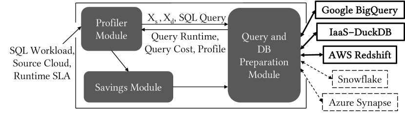
Figure 4. Arachne architecture and execution backends.

A box is drawn containing three smaller boxes, labelled Profiler Module, Savings Module, and Query and DB Preparation Module. Lines are drawn from Profile Module to Savings module, from Savings Module to Query and DB Preparation module, and back and forth between Profiler Module and Query and DB Preperation module. The line from the profiler module to the Query and DB Preperation module has a source cloud,a destination cloud and a SQL query. The reverse line has Query Runtime, Query Cost, and a Profile. The box encompassing these three modules has a line incoming to it carrying a SQL workload, a source cloud, and a runtime SLA. The query and DB prepraration module connect to 5 cloud databases. Three are bolded as they are included in the evaluation.

5. Arachne Overview

We implement Arachne, including the inter- and intra-query algorithms, in 8k lines of Python and Java. We present Arachne’s architecture in Section 5.1, the profiler in Section 5.2, and other cost-relevant implementation decisions in Section 5.3.

5.1. Overview

Figure 4 shows Arachne’s architecture. Users first execute initialize, which submits an unmodified SQL workload, stored as individual SQL files, the source execution backend where data starts, and the optional runtime constraint. Arachne implements the inter- and intra-query algorithms in the savings module. The profiler module gathers the query costs and query runtime inputs ($C_{X_{i}}$ and $R_{X_{i}}$ from Sections 3–4) so the savings module can save money and meet the runtime constraint. The preparation module prepares queries for execution in target backends. It 1) ensures that SQL queries are compatible with the syntax requirements of execution backends; 2) submits queries for execution; 3) orchestrates materializing data into portable, open-format Parquet files; and 4) migrates those Parquet files between execution backends when needed.

Execution Backends. Arachne supports two PaaS backends–AWS Redshift and Google BigQuery–so we can study per-compute and per-byte pricing models. It can also deploy DuckDB on IaaS. These backends are bolded in Figure 4. Arachne can be easily extended to support new backends, such as those in dashed lines in Figure 4.

Minimizing Infrastructure Changes. Arachne is designed to be compatible with existing ETL pipelines (and downstream BI tools and dashboards), so it moves data between source backends at runtime whenever this saves money and does so transparently to the end user. Consequently, Arachne moves data every time a workload executes (incurring costs) but does not need to handle data inconsistencies that may arise if, for example, the data were replicated in several backend systems. Exploring tradeoffs of the spectrum of solutions (keep ETLs intact and pay repeated migration costs or change ETLs, duplicate data, and incur double storage costs) is beyond the scope of this paper. Despite minimizing infrastructure changes, Arachne still requires configuration changes, e.g., to access cloud accounts. We believe this is not an important roadblock to deployment, as such credentials are frequently shared with other tools. These changes add one-time costs; in exchange, Arachne achieves large recurring savings (see Section 6).

Compliance. At a high level, Arachne is best seen as an alternative interface to the source backend. When data (or queries) cannot move (or execute) between vendors, e.g., for compliance requirements preventing data migration to a geographical area, such data can be excluded from Arachne and run using the usual interface.

Implementation. Arachne uses Apache Calcite (Begoli et al., 2018) to convert between SQL and query plans and perform query optimization. Arachne uses Apache Arrow (Apache Arrow, [n.d.]) to sample tables; the Redshift-Data API to use Redshift clusters and S3; and the Google Cloud client for Storage and BigQuery. It migrates all data at runtime.

5.2. Profiler Module

The profiler module provides the inter- and intra-query algorithms with accurate runtime, cost, and cardinality information for each query. We consider two approaches: prediction and profiling.

Why We Do Not Use Prediction in Arachne. Existing approaches to estimate operator cardinality $f_{w}$, query cost $C_{X_{i}}$, and query runtime $R_{X_{i}}$ are noisy. Cardinality estimates from query optimizers remain inaccurate (Lohman, 2014; Yang et al., 2019; Perron et al., 2019). The “cost” produced by query optimizers for a given query plan has only a relative meaning to the cost associated to other plans rather than to absolute monetary or runtime cost, making query optimizers’ cost a poor proxy for estimating runtime (Leis et al., 2015; Wu et al., 2013). Last, there are few approaches for estimating query runtime given a query plan, and existing ones often underperform, as we show in Section 6.6. However, we anticipate that continued advances in this area could replace the profiling approach we now explain.

The Profiling Approach. The profiler executes each query in each execution backend, obtaining its runtime and cost. It also gathers the output cardinality for each query operator via query profiling in DuckDB, and provides the inputs to the inter- and intra-query algorithms ($C_{X_{i}}$, $R_{X_{i}}$, and $f_{w}$ as defined in Sections 3–4). Profiling is more accurate and more costly than prediction. Profiling cost is amortized if the profiled queries execute several times without major runtime changes. This is the case for most periodic workloads (Tan et al., 2019; AWS Batch Processing, [n.d.]; BigQuery Reliability, [n.d.]), which happen to be the most relevant for saving money. Furthermore, stale profiles can still expose savings opportunities since small errors in costs do not greatly alter what queries migrate in an inter-query plan, as we illustrate in Section 6.6.

Profiling Over Samples. It is possible to reduce profiling costs by measuring runtime, cost, and operator cardinality on a workload sample and then extrapolating to the original workload size without introducing significant error. It is difficult to extrapolate query runtime from samples, which is related to the difficulty of join sampling. If the output of a join over data samples is not a sample of the true join result, we cannot accurately extrapolate runtime for the full join (Chaudhuri et al., 1999). However, profiling costs are largely in pay-per-byte pricing models and depend only on the data size. We show empirically in Section 6.6 that the profiling cost is quickly compensated by workload savings, often in less than 5 executions of the cheaper execution plan when profiling over the entire dataset and in 1–2 iterations when using a sample. For periodic workloads, we can collect profiles during iterations of the workload to reduce the net profiling costs. We see then that profiling costs are quickly compensated by workload savings.

Assigning Operator Cardinalities. To provide operator cardinality $f_{w}$ (Section 4.2), Arachne profiles queries in DuckDB as cardinality is independent of execution backend. However, DuckDB’s physical plan may not match Arachne’s internal query plan, so Arachne cannot directly match operator profiles from DuckDB onto its query plan. We observed that DuckDB does not re-order operators between SQL subqueries, so Arachne writes its query plan into SQL, with all operator trees as nested subqueries, so DuckDB’s physical plan exactly matches Arachne’s and Arachne can assign cardinalities to operators in its internal query plan.

5.3. Cost-Relevant Implementation Details

Data Transfer Between Clouds. Cloud vendors provide easy-to-use tools (e.g., AWS DataSync) to transfer data into their clouds. Beyond the egress cost of doing so, users have to pay for these tools too. Arachne implements a simple cloud transfer tool using blob storage APIs. Our tool on a GCP n2-standard-32 VM transferred a 615GB dataset for $0.58; that transfer in AWS DataSync costs $7.69.

SQL Compatibility. Arachne builds and applies text rules to ensure Arachne-produced SQL is compatible with different backend dialect rules, e.g., BigQuery requires column names to contain only alphanumerics or underscores.

Calcite Query Operators. Arachne implements its own physical node subclass and uses Calcite libraries to perform heuristic optimizations like predicate pushdown, make cuts in query plans, and assign cardinalities collected during profiling to query operators.

6. Evaluation

In this section, we answer the following research questions:

• RQ1: Does the inter-query algorithm save money? (O1)

• RQ2: Does the intra-query algorithm save money? (O2)

• RQ3: How does pricing (chosen by cloud vendors) affect inter-query savings and the runtime-cost tradeoff?

• RQ4: Profiler Microbenchmarks: How does sampling impact profiling costs and accuracy and how quickly are they compensated? Does using stale profiles diminish savings? How are savings impacted by noisy runtime estimates versus profiles?

Because Arachne can deploy DuckDB on IaaS, we also evaluate how utilizing cheaper IaaS impacts inter-query savings.

6.1. Workloads

Resource Balance Workloads. The specific balance of CPU- and IO-queries in a workload will impact savings opportunities. We use the well-known TPC-DS (Nambiar and Poess, 2006) benchmark to create three workloads each with a different balance of CPU- and IO-bound queries to explore the design space (in the original TPC-DS benchmark nearly all of the 99 queries are IO-bound). We adapt queries from LDBC, a well-known business intelligence benchmark (Szárnyas et al., 2022), to work on data from TPC-DS: we create queries to find customers related to each other by purchase history and queries to find connected components of customers for recommendation algorithms. We combine the authored CPU- and some existing IO-bound queries to create three workloads over 17 tables with different characteristics:

• W-CPU: 46 queries, about 40% of which are CPU-bound.

• W-Mixed: 49 queries, about 30% of which are CPU-bound.

• W-IO: 46 queries, about 20% of which are CPU-bound.

While there are more IO-bound queries in each workload, the CPU-bound queries consume a large amount of CPU, so overall resource consumption for each workload reflects the workload’s name. We make all workloads publicly available  for reproducibility and because they may be of independent interest to others.

Read-Heavy Workloads. We also explore skewed workloads. While nearly all TPC-DS queries are IO-bound with runtime dominated by table reads, these queries differ in runtime and complexity. To explore savings opportunities on a range of IO-bound workloads we create 24 workloads called the Read-Heavy workloads from TPC-DS, which contains 24 tables and 99 queries, by removing one table from the TPC-DS dataset. This creates a 23-table dataset with a subset of the original 99 queries, on average about 80 queries. Each workload is named by the alphabetical order of the table that was removed to generate it, e.g., the workload created by removing the first table alphabetically, call_center, will be named Read-Heavy 0.

LDBC. Additionally, we use queries written on the LDBC Social Network Benchmark-Business Intelligence (SNB-BI) dataset (Szárnyas et al., 2022).

For RQ1 and RQ3 we use the Resource Balance and Read-Heavy Workloads. For RQ2, we use TPC-DS queries and author queries on TPC-DS and LDBC. We explain these in detail in that section.

6.2. Experimental Setup

PaaS Execution Backends. We use Google BigQuery (pay-per-byte) and AWS Redshift (pay-per-compute) as popular representatives of each pricing model. In Redshift cluster size impacts cost and performance, so we explore the G$\rightarrow$A1, G$\rightarrow$A4, G$\rightarrow$A8 setups where data starts in BigQuery (G) and we consider migrating to a 1-, 4-, or 8-node ra3.xlplus Redshift cluster respectively ($\rightarrow$A1, $\rightarrow$A4, or $\rightarrow$A8; the arrow indicates the migration direction). We explore the A4$\rightarrow$G setup where data starts in a 4-node ra3.xlplus Redshift cluster and could migrate to BigQuery. We optimize our Redshift and BigQuery setup per docs and best practices (Scaer et al., 2020; Burman et al., 2022; BigQuery Optimizing, [n.d.]; Sharma and Fu, [n.d.]).

Data Format and Storage. We store intermediate data in Parquet files (Apache Parquet, [n.d.]) with Snappy compression (Snappy, [n.d.]). All cloud databases we use are compatible with open data formats (Databricks Data Lakes, [n.d.]; Prasad, 2022). We create external tables in BigQuery pointing to the Parquet files in blob storage. We also consider data loaded into BigQuery. Redshift loads Parquet files from S3. The compression of data saves migration costs, and all in-flight compression occurs during materialization from pay-per-compute databases and is billed as runtime cost.

Where Data Is Initially Stored. For the Resource Balance Workloads, we consider G$\rightarrow$A4 and A4$\rightarrow$G. With current prices, Redshift is significantly cheaper than BigQuery for IO-skewed workloads and queries. As such, we consider only G$\rightarrow$A1, G$\rightarrow$A4, G$\rightarrow$A8 for the Read-Heavy workloads to evaluate O1 and only consider DuckDB and BigQuery on data stored in GCP to evaluate O2, as there are few savings opportunities if data starts in Redshift.

How Workloads Are Executed. Batch, analytic workloads like those in this evaluation are often executed serially but can also be submitted all at once to a system (IBM Serial Batch, [n.d.]; AWS Batch, [n.d.]). For pay-per-byte systems like BigQuery, this has no impact on workload cost, only runtime. For pay-per-compute systems like Redshift, this also impacts costs. Redshift’s REST API, the Redshift Data API (BatchExecuteStatement, [n.d.]) offers BatchExecuteStatement which executes a list of SQL statements one at a time in a single transaction.

Metrics. We measure monetary cost in US dollars and runtime in time units. We account for all applicable cloud costs (see Section 2.1.2) and use cloud prices as of February’24 in Table 1. We validate our results by checking the breakdown of charges in our account from cloud vendors. We create VMs in the same cloud region as blob storage buckets to avoid regional transfer costs and utilize data compression to reduce migration costs.

Runtime Constraint. We assume that there are no runtime constraints and concentrate on exploring cost savings without imposing arbitrary runtime constraints that do not add any additional insight.

6.3. RQ1. Inter-Query Processing

We now explore O1. First, we evaluate the cost opportunities of the inter-query algorithm across the three Resource Balance Workloads (Section 6.3.1) and the IO-skewed Read-Heavy workloads (Section 6.3.2). Then, we leverage that Arachne can deploy DuckDB on IaaS to evaluate how that impacts savings (Section 6.3.3).

6.3.1. Resource Balance Workloads

We run the inter-query algorithm on W-CPU, W-IO, and W-Mixed in G$\rightarrow$A4 and A4$\rightarrow$G and evaluate multi-cloud savings. First, we provide an overview of the results before presenting an in-depth breakdown of costs.

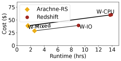
(a) 1TB A4$\rightarrow$G

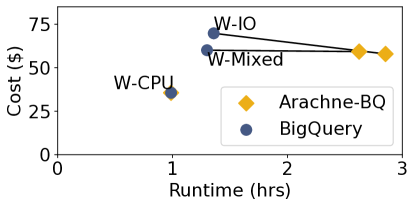
(b) 1TB G$\rightarrow$A4

Figure 5. (1TB A4$\rightarrow$G, G$\rightarrow$A4) Cost (USD) vs runtime (hours) for W-CPU, W-IO, and Mixed workload compositions

There are two plots, one where data begins in AWS and one where data begins in GCP. When starting in AWS, Arachne’s plans are both faster and cheaper. When starting in GCP, Arachne’s plans for two workloads are cheaper but slower. For the third workload Arachne saves no money or time.

Resource Balance Workload Overview. In Figure 5 we compare the runtime (hours) on the x-axis and cost (USD) on the y-axis of Arachne’s execution plan to a baseline that executes the workload in the starting backend. In Figure 5a, data starts in Redshift. There are three red dots, one for each workload, which represent the cost and runtime of executing that workload in Redshift. The yellow dots represent the runtime and cost of executing that workload with Arachne. A line connects each yellow dot to its corresponding red dot according to the workload. In Figure 5b, data starts in BigQuery (blue dots) instead of Redshift.

In 5 out of the 6 workloads Arachne finds cheaper plans: all lines decrease from the starting cloud baseline unless Arachne has chosen the baseline execution plan, and the degree of its reduction corresponds to monetary savings. For A4$\rightarrow$G in Figure 5a, Arachne chooses multi-cloud plans for all three workloads as there are enough CPU-bound queries to make migration cost-effective. Arachne saves 27% on W-IO and 35% on W-Mixed and W-CPU over the Redshift baseline. Arachne saves less money for W-IO because there are more IO-bound queries that favor Redshift’s per-second pricing model. In G$\rightarrow$A4 in Figure 5b, Arachne executes W-CPU entirely in BigQuery, so those two dots are directly on top of each other. Since W-Mixed and W-IO contain more IO-bound queries, Arachne saves 1.35% on W-Mixed and 17% on W-IO by migrating IO-bound queries to Redshift. Because W-IO has more IO-bound queries, the margin of savings is larger for W-IO than for W-Mixed.

Both W-Mixed and W-CPU include a very CPU-bound query, which groups customers by spending history for recommendations. It runs in 6 hours and costs $25.84 in Redshift, while in BigQuery it runs in 3.5 minutes and costs $1. Other CPU-bound queries are similarly faster and cheaper in BigQuery. Consequently, in the A4$\rightarrow$G setup in Figure 5a, baseline costs for W-Mixed and W-CPU are similar, and Arachne chooses similar multi-cloud plans for both workloads that are faster and cheaper than the Redshift baseline.

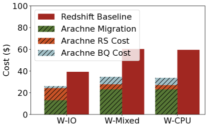
(a) A4$\rightarrow$G: Data Starts in Redshift

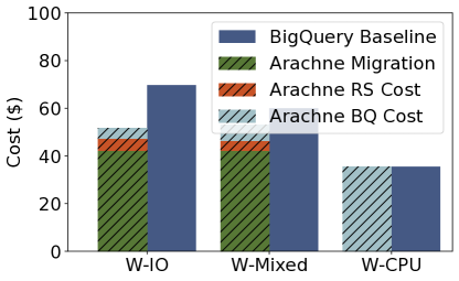
(b) G$\rightarrow$A4: Data Starts in BigQuery

Figure 6. (1TB) Arachne migration costs, cost of queries moved, and cost of queries remaining versus baseline.

Two plots are shown, each depicting three pairs of bars. One plot where data starts in AWS and one where data starts in GCP. For each pair of bars, the right bar is a solid color and represents the baseline. The left bar has diagonal lines through it and is broken up into three categories each with their own color: Arachne Migration, Arachne RS cost, and Arachne BQ cost.

Resource Balance Workload Cost Breakdown. We divide costs for Arachne into (1) migration costs, (2) the cost of queries which migrated, and (3) the cost of queries which remained in the source backend. In Figure 6a we breakdown costs for plans shown in Figure 5a and in Figure 6b we breakdown costs for plans in Figure 5b. Diagonal lines are drawn through bars showing Arachne’s plans.

Table 2. Inter-query plan-type by setup at 1TB and 2TB.

Setup	Arachne	Multi	GCP	AWS	Total
1TB, G$\rightarrow$A1, $\rightarrow$A4, $\rightarrow$A8	23	6	1	17	24
2TB, G$\rightarrow$A1	22	4	1	19	24
2TB, G$\rightarrow$A4	22	3	2	19	24
2TB, G$\rightarrow$A8	22	4	2	18	24

In Figure 6b, W-CPU Arachne’s bar is equal to the BigQuery baseline. If the source pricing model is already favorable for a workload, Arachne will keep all data in the starting cloud. For all other plans in Figure 6, multi-cloud savings are driven by the significantly lower execution cost for queries that migrated to a favorable pricing model versus their baseline cost. In Figure 6, the difference in query execution costs is the baseline (right) bar minus the blue portion of Arachne’s bar, which represents the cost of queries remaining, presenting an enormous savings opportunity. Exorbitant migration costs make up the majority of Arachne’s costs for multi-cloud plans. Egress is 90% of all migration costs–note that egress out of GCP is $120/TB while egress out of AWS is $90/TB–loading data into Redshift is 5–8% of migration costs, and the rest is the cost of blob storage and data retrieval.

6.3.2. Read-Heavy Workloads

Does Arachne save money on skewed workloads? We first summarize the results before zooming in on a few interesting workloads to understand the cost and runtime.

Read-Heavy Overview. Table 2 presents the outcomes in setups G$\rightarrow$A1, G$\rightarrow$A4, G$\rightarrow$A8. The Arachne column indicates workloads where Arachne saves money over the BigQuery baseline. Across 144 workloads–48 workloads in 3 setups–only 6/144 remain in BigQuery where the Arachne saves no money. For workloads with cheaper plans, in Multi plans some tables migrate to Redshift, and in AWS plans all tables migrate to Redshift. Since Read-Heavy workloads are IO-bound, the savings of moving queries to Redshift compensate for migration costs. That even 6 of these IO-skewed workloads remain in BigQuery demonstrates that egress costs are a massive barrier to data movement.

At 2TB, we see that from G$\rightarrow$A1 to G$\rightarrow$A4 one Multi plan flips to GCP and from G$\rightarrow$A4 to G$\rightarrow$A8 one AWS plan flips to Multi. The 4$\times$ cost of G$\rightarrow$A4 doesn’t reduce runtime by 4$\times$, decreasing savings. If clusters are overprovisioned or underutilized, query savings will diminish even with highly IO-bound workloads.

Arachne saves up to 57.4% on a single workload.Of the 29 multi-cloud plans, most achieved 35%–50% savings. 9 saved 2%-8%, while 1 saved less than 1%. These plans save money by migrating queries to their most beneficial pricing model.

Multi Plan Analysis. We now focus on Multi plans which run queries on both BigQuery and Redshift to show the opportunities of combining price-per-byte and price-per-compute pricing models.

As in Figure 5, Figure 7 plots workload cost versus runtime for Multi plans. Blue dots represent BigQuery baseline plans while yellow dots represent Arachne plans. Dots corresponding to the same workload are connected with a line. These plans achieve up to 54% savings and over 35% for most workloads. 2 workloads at 1TB and 1 workload at 2TB save between 2 and 8%. 1 workload at 2TB G$\rightarrow$A1 saves less than 1%, as Arachne migrates very few queries and tables which yield marginal savings.

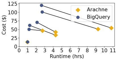
(a) 1TB G$\rightarrow$A1

(b) 2TB G$\rightarrow$A1

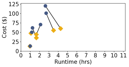
(c) 1TB G$\rightarrow$A4

(d) 2TB G$\rightarrow$A4

(e) 1TB G$\rightarrow$A8

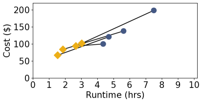
(f) 2TB G$\rightarrow$A8

Figure 7. Cost (USD) vs runtime (hours) for 1–2TB datasets with Multi plans over Redshift and BigQuery.

Six plots are shown in two sets of 3. Each set shows three different setups, one using a 1 node Redshift cluster, one using a 4 node Redshift cluster, and one using an 8 node Redshift cluster. The first set is 1TB dataset and the second set is a 2TB dataset. There are yellow dots and corresponding blue dots that are connected to a yellow dot by a line. For 1TB and 1 node, all Arachne plans are slower and cheaper, except for one which is negligibly cheaper and slower. For 1TB and 4 nodes, 2 workloads are cheaper and faster, 2 are cheaper and slower, and 2 have marginal differences. For 1TB and 8 nodes, all workloads are both cheaper and faster. For 2TB and 4 nodes the workloads are cheaper and nearly twice as fast. At 2TB and 8 nodes many workloads are nearly 3 times faster.

In Figure 7, the BigQuery baseline is faster than Arachne’s plan because G$\rightarrow$A1 does not exploit all the parallelism available in the workload. At G$\rightarrow$A4 we see that Arachne’s plan is cheaper and closer in runtime to the baseline, and is both cheaper and faster in G$\rightarrow$A8. In larger clusters, loading times decrease, and Redshift completes the workloads faster (and cheaper) than BigQuery. At 2TB, the trends are similar to 1TB except that now Arachne is both cheaper and faster than BigQuery even in the G$\rightarrow$A4 case.

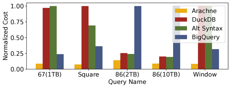
Figure 8. Query costs normalized to most expensive plan for Arachne’s intra-query plan vs BigQuery, DuckDB, and DuckDB with Arachne-produced text (Alt Syntax).

Shows 5 sets of 4 bars. Plots normalized cost on the y-axis. Each set represents a different query. Each of the 4 bars represents a different baseline. The yellow bar representing Arachne is the lowest in all 5 cases. Which baseline is the most expensive changes between queries. The yellow bar is 30-35 times cheaper than the most expensive baseline in all cases and at least 2-3 times cheaper than the next cheapest baseline.

BigQuery Internal Tables. Loading data into BigQuery is free but significantly increases runtime; loading 1TB took 12 minutes whereas creating external tables took only 20 seconds. Data is stored in a closed format and only accessible via their SQL interface, which incurs query processing costs, or BigQuery’s Storage Read API (Google BigQuery Storage Pricing, [n.d.]); both are much more expensive than the blob storage API costs.

For queries over internal tables, BigQuery charges once for each table scanned, even if the table is scanned multiple times in the query. For queries over external tables, BigQuery charges for each table scan operator, even if multiple operators scan the same table. So the same query will scan fewer bytes and cost less when data is stored internally. We run the inter-query algorithm on G$\rightarrow$A1, G$\rightarrow$A4, and G$\rightarrow$A8 with data stored internally. There are 3-5 multi-cloud workloads in each setup saving 3–20% and 2 with negligible savings, similar to the external case, because of high BigQuery prices and the large IO-bound savings in the Read-Heavy workloads. These savings margins are smaller due to the fewer bytes billed.

6.3.3. Extending Arachne with IaaS+DuckDB

We now explore the cost differences between PaaS (the databases evaluated above) and a new execution backend that deploys DuckDB on a GCP VM, where data starts, to avoid egress costs. The VM costs $1.49/hour with 16 vCPU, 190GB RAM, and 1TB disk to run memory-intensive queries.

This VM did not have enough memory to run all queries. To concentrate on studying the effect of IaaS, we edited the queries slightly, replacing WITH clauses with CREATE TABLE AS clauses so that intermediate tables are offloaded to disk. While this may increase query runtime it allowed the query to complete so we could proceed with our study. We only consider queries which execute in all execution backends.

In this setup, Arachne does not migrate any queries to Redshift, as IaaS lowered query costs enough that migration is not worthwhile. However, Arachne still achieves up to 55% savings over the pay-per-byte BigQuery (PaaS) baseline by utilizing cheaper, pay-per-compute IaaS which dramatically reduces costs for the IO-bound workloads. Hence, Arachne can identify opportunities and achieve significant savings with a transparent deployment of DuckDB on IaaS, all without separate user setup, deployment, or maintenance.

6.3.4. Summary

Arachne successfully exploits the inter-query algorithm (O1), even in highly skewed workloads if the source pricing model is ineffective for it. Arachne chooses multi-cloud plans saving 35%–56% in most cases by using multiple pricing models.

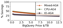
(a) A4$\rightarrow$G BigQuery Price

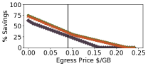
(b) A4$\rightarrow$G Egress Price

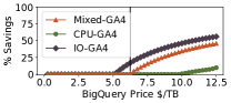
(c) G$\rightarrow$A4 BigQuery Price

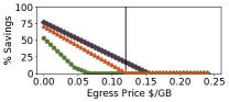
(d) G$\rightarrow$A4 Egress Price

Figure 9. (G$\rightarrow$A4, A4$\rightarrow$G 1TB) % savings for inter-query plans vs. BigQuery or egress prices on Resource Balance Workloads

Four plots showing relative savings versus varying either egress price or BigQuery price in 2 different setups. As egress price increases eventually all savings go to zero. When starting in BigQuery, very low BigQuery prices cause no savings but as prices increase there is a point where all workloads save money via inter-query plans. WHen data starts in AWS, there is smaller changes with savings as BigQuery price increases, and it is always above zero.

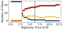
(a) 1TB Varying BigQuery Price

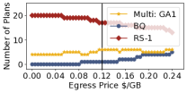
(b) 1TB Varying Egress Price

Figure 10. (G$\rightarrow$A1 1TB) Inter-query results varying either BigQuery or egress price on Read-Heavy Workloads

As BigQuery price increases, the number of BQ-only plans drops precipitously while the number of AWS-only plans increase. The number of multi-plans is nonzero and increases for a while but then settles and fluctuates slightly. As egress price increases, there are more BQ-only plans and fewer AWS-only plans while the number of multi-cloud plans varies somewhat but stays relatively consistent.

Table 3. Absolute baseline and Arachne intra-query costs.

Query	Arachne	BigQuery	DuckDB	Alt Syntax
67	$1.83	$4.9981	$20.4027	$21.0109
Square	$0.005507	$0.0156	$0.07321	$0.05069
86 (2TB)	$0.089574	$0.62853	$0.1605	$0.15144
86 (10TB)	$0.278728	$3.142	$0.63195	$0.60877
Window	$0.311999	$1.1791	$3.7159	$3.7159

6.4. RQ2. Intra-Query Processing

In this section, we explore opportunity O2 via the intra-query algorithm. These opportunities are significant but occur less often than O1, so we report results for five queries that produced a cheaper intra-query plan and analyze the characteristics of these queries.

Queries. Query 67 and window are run on a 1TB TPC-DS dataset and query 86 is run on a 2TB and 10TB TPC-DS dataset. The window query performs several joins and group-bys and executes a complex window operation on the result. The square query, run on 100GB LDBC-SNB dataset, finds squares in social media graphs, e.g., a path from person A to B to C to D and back to A.

Experimental Setup. Data starts in BigQuery, and we consider intra-query plans between BigQuery (pay-per-byte) and DuckDB (pay-per-compute) on a GCP VM. Expensive egress fees restrict data movement and eliminate intra-query opportunities across multiple clouds, so we consider GCP-only intra-query plans. We pay profiling costs to copy data to the VM and execute queries in BigQuery and DuckDB, gathering cost, runtime, and operator cardinality. Arachne converts its internal query plan into SQL to execute subqueries, but we observe that alternate SQL texts for the same logical query can cause the optimizer to choose different physical plans, affecting runtime and cost. To isolate this factor, we consider a third baseline, called Alt Syntax, which is the cost of executing the initial query rewritten by Arachne in DuckDB.

Results. Figure 8 shows the costs for Arachne’s intra-query plan and the baselines normalized to the most expensive baseline for each query. Arachne’s plans save 2–5$\times$ compared to the next cheapest baseline and orders of magnitude compared to the most expensive baseline, showing the cost saving potential of O2. We normalize values to emphasize the relative savings as the absolute savings are small because out-of-memory errors on larger datasets prevented us from using longer-running queries. We show the absolute numbers in Table 3 and note that relative costs better represent total savings, as the total savings are query savings multiplied by the number of times a query executes. While intra-query plans sometimes run slower than the fastest baseline (shown in Table 4), this potential slowdown is tolerable if the query is run in a latency-insensitive, periodic workload such as a nightly analytics workload.

Table 4. Runtime (seconds) for baselines and Arachne plans.

Query	Arachne	BigQuery	DuckDB	Alt Syntax
67	4059.96	555.333	50655.30	51107.595
Square	188.226	14.569	168.727	113.961
86 (2TB)	171.051	206.045	381.271	359.023
86 (10TB)	580.898	423.063	1527.825	1471.458
Window	624.970	82.155	9038.641	8954.334

Common Characteristics. These queries first join many tables (IO-bound) followed by a window or self-join (CPU-bound). Queries with these stages are good candidates for the intra-query algorithm.

Summary. There are fewer situations where O2 saves money versus O1, but when opportunities exist, the relative savings are significant, especially for queries with the structure discussed above. Profiling costs for 3/5 queries are earned back in under 25 iterations. Query 67 and window are earned back in 28 and 46 iterations and cost $85.68 and $40.18. The savings achieved are significant and compensate for incurred profiling costs. Re-profiling may be required more frequently for O2 than O1, increasing costs. However, the sizable savings margin can quickly earn back that up-front cost.

6.5. RQ3. Simulating Different Cloud Costs

So far, the results shown assume cloud vendor prices as of February’24. In this section, we use profiled inputs (discussed in Section 5.2) that are not affected by cloud vendor prices and simulate cloud prices by varying the price inputs to the inter-query algorithm. We vary the price-per-byte (BigQuery price) and egress price from the source execution backend and run the inter-query algorithm on the Read-Heavy (RH) workloads and Resource Balance Workloads (RBW) to see how varying prices impacts savings. Vertical lines indicate the current price. We use the plan types as in Section 6.3–GCP, AWS, or Multi. For RBW, we show percent savings (Figure 9) versus the price being varied in A4$\rightarrow$G and G$\rightarrow$A4. Figure 10 shows plan types for RH in G$\rightarrow$A1 at 1TB; trends are similar in G$\rightarrow$A4 and G$\rightarrow$A8 and at 2TB. The main takeaways are:

• Inter-query savings (O1) are robust to changes in prices even for heavily IO-bound workloads.

• Reducing BigQuery price by 40% to $3.75/TB keeps most RH plans in BigQuery. At 2TB the necessary price reduction increases because potential savings grow as dataset size grows.

• For RBW, in A4$\rightarrow$G BigQuery price does not impact plan type but slightly reduces savings. In G$\rightarrow$A4, reducing prices by 20% to $5/TB keeps all plans in BigQuery.

• At low egress prices, Multi plans are the cheapest option for 4/24 RH workloads in 1–2TB and all RBWs in A4$\rightarrow$G. Even if cloud vendors lower financial barriers to data movement, money-saving, inter-query opportunities (O1) still exist.

• High egress prices lock-in all RBW plans to their starting cloud. For RH, multi-cloud plans still exist, so savings achievable by using multiple pricing models outpace egress costs.

Runtime vs. Cost Tradeoffs. To observe how cloud prices impact cost and runtime tradeoffs, we zoom in on Read-Heavy 22 at G$\rightarrow$A4 1TB and show the percent savings and percent speedup over the baseline vs. BigQuery and egress prices in Figure 11. Negative percent speedup indicates that Arachne’s plan is slower.

A small increase in BigQuery price from $6.25/TB to $7/TB causes Arachne to migrate more tables in a multi-cloud plan, which runs longer than the baseline but achieves greater savings. A slight decrease of egress cost to $0.105/GB from $0.12/GB yields a similar result for the same reasons, as migrating more tables increases savings but also runtime. At many other prices the Arachne’s plan is both cheaper and faster. Figure 11 illustrates how the specific tradeoff of runtime and cost is impacted by cloud vendor prices.

Conclusions. Overall, we see that our results are not brittle to price changes: some queries are simply cheaper in different pricing models and prices dictate how large savings are and how large barriers to migration are. More importantly, they show the power platforms have to lock in workloads by adjusting prices slightly; this anti-competitive restriction should be concerning to all of us.

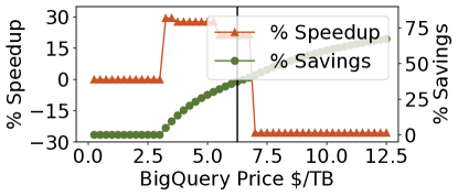
(a) 1TB G$\rightarrow$A4 Varying BigQuery Price

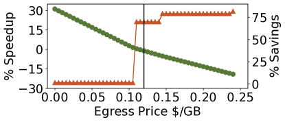
(b) 1TB G$\rightarrow$A4 Varying Egress Price

Figure 11. (1TB G$\rightarrow$A4) % Savings and speedup of Arachne for Read-Heavy 22 vs. BigQuery and egress price.

Shows two plots for 1TB and starting in GCP and going to an A4 setup. As BigQuery price increases the savings go from 0 to about 75 percent in a curve that is concave down. Runtime is the same when savings are 0, is faster by about 30 percent for lower amounts of savings, and then is 30 percent slower for the plans with greater savings at higher BigQuery prices. When increasing egress price savings start at about 75 percent and decrease, roughly concave up, down to close to 0. The larger savings plans are about 30 percent slower but then get faster as savings decrease, going up to between 15 and 30 percent faster.

6.6. RQ4: Profiling Cost Microbenchmarks

Gathering inter-query inputs (Section 5.2) incurs significant profiling costs. We show how stale profiles impact savings (Section 6.6.1), how profiling over samples lowers profiling costs (Section 6.6.2), and how noisy runtime estimates impact savings (Section 6.6.3)

6.6.1. Impact of Re-profiling

We first study the savings impact of using stale profiles as data changes. We create 7 datasets with sizes from 100–1200GB with the official TPC-DS generator. A TPC-DS dataset reflects a database at a moment in time for a retail supplier. While tables tracking sales and returns only grow with overall data size, other tables tracking inventory or customers grow and shrink as overall data size increases, per the TPC-DS specification (TPC-DS, [n.d.]).

We let each data size be the state on a given day over 7 days. In Figure 12 we compare four execution strategies in G$\rightarrow$A4 as data changes. We compare the BigQuery baseline (BQ), against two Arachne strategies: profiling only on day 1 (A-1P) and using that profile for days 2–7; and profiling as soon as data changes (the solid red line, A-RP). A-1P and A-RP include profiling costs. Finally, we show the cost of A-RP without profiling costs as the dotted red line.

We compare these strategies on Read-Heavy 2 which showed the largest gap between A-1P and A-RP. While A-RP is cheaper over time, it is at most 2% cheaper than A-1P. Daily re-profiling costs make A-RP far more expensive than BQ. A-1P quickly compensates for profiling costs and saves significantly over BQ. A-1P’s stale profile still captures which queries are cheaper in which backend, so small errors in the profile do not appreciably diminish savings.

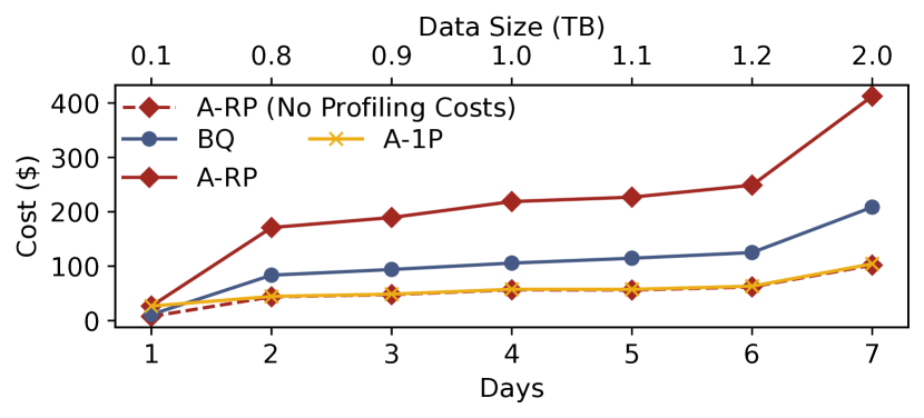
Figure 12. (G$\rightarrow$A4) Cost (USD) vs days and data size (TB)

One plot showing the cost of four different execution strategies versus time in days. Each day has a corresponding data size shown on the upper x-axis. Days are numbered 1 to 7. Day 1 has 0.1TB, Day 2 has 0.8TB, Day 3 has 0.9TB, Day 4 has 1.0TB, Day 5 has 1.1TB, Day 6 has 1.2TB, and Day 7 has 2TB. All four points are clustered together with similar costs on Day 1. The red line for A-RP is the highest across all days, and from day 2 to 7 is significantly higher than the rest. The blue line representing the BigQuery baseline is always cheaper than that but always second most expensive. The yellow line is marginally more expensive than the dotted red line, but is consistently the cheapest of the four.

6.6.2. Sampling

We now show how sampling reduces profiling costs with low error. While estimating runtime from samples is difficult for some queries (Chaudhuri et al., 1999; Liang et al., 2021; Yang et al., 2019), most profiling cost are from pay-per-byte pricing models, where runtime does not affect cost.

We show cost and estimation error for samples of 15, 25, 50, and 100% of data in Table 5. When profiling over all data, 20/24 workloads earn back profiling costs in 4 iterations. Small samples estimate the inputs well and in most cases lower the number of needed iterations to 1–2. Read-Heavy 7 chooses a GCP-only plan so achieves no savings. Read-Heavy 17 only achieves marginal savings and needs many iterations, though sampling lowers the net cost of profiling. We do not claim that sampling is the best approach, only that it cheapens profiling. More sophisticated approaches, e.g., using parameterized cost models to sample non-linear operators (Li et al., 2019) can further reduce error, which we leave for future work.

6.6.3. Profiling versus Runtime Estimation

We estimate query runtimes in Redshift by training a Kernel Canonical Correlation Analysis (KCCA) model, as proposed by Ganapathi et. al. (Ganapathi et al., 2009) in 2009. KCCA finds correlated clusters of training features and labels to make predictions. However, hardware advances over 15 years mean that queries run much faster, so most training points are clustered together despite the size and diversity of the training set, lowering the reproduced model’s accuracy. Nonetheless, we created 2842 training queries as the original 3102 queries used were not available after reaching out to the authors. We used a 1GB TPC-DS dataset and also ran some queries on 100GB and 1TB datasets to get a broader range of runtimes. We make a significant effort to replicate the setup and create a runtime estimation method for SQL queries.

Inter-query plans using runtime estimates are 66% more expensive than plans using profiles on W-Mixed in the A1$\rightarrow$G setup and 13% more expensive in G$\rightarrow$A1 when they cost the same as the baseline. Noisy estimates result in Arachne missing valuable savings opportunities and greatly diminish savings margins, illustrating the detrimental impact of estimation on inter-query savings.

7. Related Work

Other Cloud Databases. Many other cloud and third-party databases scan cloud storage like Snowflake, Azure Synapse, Trino, Apache Hive, Amazon Athena, and SparkSQL (Dageville et al., 2016; Azure Synapse, [n.d.]; Aguilar-Saborit et al., 2020; Presto, [n.d.]; Thusoo et al., 2010b; Amazon Athena, [n.d.]; Armbrust et al., 2015). These databases use per-second billing (Presto, Hive, SparkSQL), per-byte billing (Athena), or some combination of the two. While we could have used other systems in our evaluation, Google BigQuery and AWS Redshift effectively represent both pricing models across clouds, enabling us to evaluate opportunities O1–O2.

Cloud Cost Savings. Prior work on money savings focuses on scheduling algorithms (Wu et al., 2015), exploring cost sources in different execution backends (Tan et al., 2019), or using S3 Select (Hunt, 2017) to speed up queries and lower costs (Yu et al., 2020). Leis and Kuschewski model per-second costs for cloud workloads (Leis and Kuschewski, 2021). Recent work has also focused on achieving savings using spot instances (Wu et al., 2024), minimizing network egress prices (Wooders et al., 2024), and finding cheaper configurations for cloud deployments (Bang et al., 2024). To the best of our knowledge, Arachne is the first effort to systematically explore savings opportunities for analytical queries by using multiple databases with different pricing models.

Sample %	15			25			50			100
Dataset	Cost	Iter	Error	Cost	Iter	Error	Cost	Iter	Error	Cost	Iter	Error
Read-Heavy 0	30.39	1	0.02	49.33	1	0.03	94.2	2	0.03	177.19	3	0.0
Read-Heavy 1	30.04	1	0.02	48.71	1	0.03	92.97	2	0.03	174.93	3	0.0
Read-Heavy 2	27.41	1	0.02	44.49	1	0.03	84.54	2	0.04	157.69	3	0.0
Read-Heavy 3	17.54	1	0.03	28.17	1	0.04	53.45	2	0.05	97.78	4	0.0
Read-Heavy 4	25.6	1	0.03	41.33	2	0.04	78.14	2	0.04	143.91	4	0.0
Read-Heavy 5	26.12	1	0.03	42.24	2	0.03	80.01	2	0.04	148.96	4	0.0
Read-Heavy 6	27.55	1	0.02	44.49	1	0.03	84.55	2	0.04	157.9	4	0.0
Read-Heavy 7	13.86	N/A	0.06	21.87	N/A	0.09	39.3	N/A	0.1	65.17	N/A	0.0
Read-Heavy 8	28.25	1	0.02	45.62	1	0.03	86.77	2	0.03	162.65	4	0.0
Read-Heavy 9	30.0	1	0.02	48.62	1	0.03	92.77	2	0.03	174.48	3	0.0
Read-Heavy 10	30.16	1	0.02	48.91	1	0.03	93.36	2	0.03	175.64	3	0.0
Read-Heavy 11	19.26	5	0.04	30.62	8	0.05	57.13	15	0.06	101.91	26	0.0
Read-Heavy 12	28.97	1	0.02	46.91	1	0.03	89.32	2	0.03	167.45	3	0.0
Read-Heavy 13	29.81	1	0.02	48.28	1	0.03	92.13	2	0.03	173.19	3	0.0
Read-Heavy 14	30.42	1	0.02	49.44	1	0.03	94.21	2	0.03	177.39	3	0.0
Read-Heavy 15	22.77	2	0.03	36.53	2	0.04	68.43	4	0.04	126.6	7	0.0
Read-Heavy 16	26.54	1	0.02	42.94	1	0.03	81.52	2	0.04	152.01	4	0.0
Read-Heavy 17	8.65	26	0.05	13.47	40	0.06	24.84	74	0.08	42.85	127	0.0
Read-Heavy 18	29.78	1	0.02	48.31	1	0.03	91.96	2	0.03	173.15	3	0.0
Read-Heavy 19	30.06	1	0.02	48.85	1	0.03	93.03	2	0.03	174.9	3	0.0
Read-Heavy 20	30.31	1	0.02	49.17	1	0.03	93.88	2	0.03	176.83	3	0.0
Read-Heavy 21	28.35	1	0.02	46.01	1	0.03	87.54	2	0.03	164.02	3	0.0
Read-Heavy 22	20.58	1	0.03	33.3	2	0.04	63.02	3	0.05	114.34	5	0.0
Read-Heavy 23	29.89	1	0.02	48.48	1	0.03	92.51	2	0.03	173.99	3	0.0

Table 5. Profiling costs, iters to earn back profiling costs, and est. error for 15, 25, 50, and 100% samples (G$\rightarrow$A1 1TB).

Other Complementary Optimizations. Other prior work saves money through semantic caching and distributed query optimization techniques  (Dar et al., 1996; Durner et al., 2021; Kotidis and Roussopoulos, 1999; Perez and Jermaine, 2014), optimizing data placement (Kossmann et al., 2000; Polychroniou et al., 2018), and view selection and materialization in data warehouses (Nadeau and Teorey, 2002; Chirkova et al., 2002; Auto-MV, [n.d.]; Redshift Spectrum, [n.d.]). These efforts save costs within a single pricing model and can be applied to databases prior to our analysis across multiple pricing models; for that reason they complement our research.

Cloud-Agnostic Query Execution. Recent position papers have emphasized the need to build cloud-agnostic data infrastructure. Berkeley’s Sky Computing vision outlines opportunities for multi-cloud workload execution (Chasins et al., 2022). Our work on Arachne emphasizes cost savings across pricing models.

Federated Query Execution. Some prior work improves performance for federated queries by using metadata from federated sources (Charalambidis et al., 2015), by improving query planning for federated queries (Ewen et al., 2006), or by building full federated query systems (Josifovski et al., 2002). These works do not aim to save money and consider a single execution backend and multiple storage endpoints, while Arachne uses multiple execution backends with different pricing models to save money.

8. Conclusion

This paper presents, exploits, and evaluates two money saving opportunities for cloud analytical workloads. The key is to schedule queries based on the resources they consume onto beneficial pricing models offered by cloud vendors. We measure hard-to-estimate query information, implement the inter- and intra-query algorithms, and use IaaS to save money, all while honoring runtime constraints.

We hope this work will encourage further investigation into multi-cloud savings opportunities. Ideally, this line of work fosters competition between cloud vendors, driving down prices and benefiting users. Cloud vendors may, however, simply modify prices to prevent data movement and lock-in users. Even in extreme situations multi-cloud opportunities exist, and we hope that cloud vendors choose to reduce costs for users and pay for the revenue loss by becoming more energy-efficient to lower internal costs.

References

- (1)
- Aguilar-Saborit et al. (2020) Josep Aguilar-Saborit, Raghu Ramakrishnan, Krish Srinivasan, Kevin Bocksrocker, Ioannis Alagiannis, Mahadevan Sankara, Moe Shafiei, Jose Blakeley, Girish Dasarathy, Sumeet Dash, Lazar Davidovic, Maja Damjanic, Slobodan Djunic, Nemanja Djurkic, Charles Feddersen, Cesar Galindo-Legaria, Alan Halverson, Milana Kovacevic, Nikola Kicovic, Goran Lukic, Djordje Maksimovic, Ana Manic, Nikola Markovic, Bosko Mihic, Ugljesa Milic, Marko Milojevic, Tapas Nayak, Milan Potocnik, Milos Radic, Bozidar Radivojevic, Srikumar Rangarajan, Milan Ruzic, Milan Simic, Marko Sosic, Igor Stanko, Maja Stikic, Sasa Stanojkov, Vukasin Stefanovic, Milos Sukovic, Aleksandar Tomic, Dragan Tomic, Steve Toscano, Djordje Trifunovic, Veljko Vasic, Tomer Verona, Aleksandar Vujic, Nikola Vujic, Marko Vukovic, and Marko Zivanovic. 2020. POLARIS: the distributed SQL engine in azure synapse. Proceedings of the VLDB Endowment 13, 12 (aug 2020), 3204–3216. https://doi.org/10.14778/3415478.3415545
- Amazon Athena ([n.d.]) Amazon Athena [n.d.]. Amazon Athena - Serverless Interactive Query Service - Amazon Web Services. Retrieved 2023-11-21 from https://aws.amazon.com/athena/
- Apache Arrow ([n.d.]) Apache Arrow [n.d.]. Apache Arrow. Retrieved 2024-02-13 from https://arrow.apache.org
- Apache Parquet ([n.d.]) Apache Parquet [n.d.]. Apache Parquet. Retrieved 2022-12-17 from https://parquet.apache.org/
- Armbrust et al. (2015) Michael Armbrust, Reynold S. Xin, Cheng Lian, Yin Huai, Davies Liu, Joseph K. Bradley, Xiangrui Meng, Tomer Kaftan, Michael J. Franklin, Ali Ghodsi, and Matei Zaharia. 2015. Spark SQL: Relational Data Processing in Spark. In Proceedings of the 2015 ACM SIGMOD International Conference on Management of Data (Melbourne, Victoria, Australia) (SIGMOD ’15). Association for Computing Machinery, New York, NY, USA, 1383–1394. https://doi.org/10.1145/2723372.2742797
- Armenatzoglou et al. (2022) Nikos Armenatzoglou, Sanuj Basu, Naga Bhanoori, Mengchu Cai, Naresh Chainani, Kiran Chinta, Venkatraman Govindaraju, Todd J. Green, Monish Gupta, Sebastian Hillig, Eric Hotinger, Yan Leshinksy, Jintian Liang, Michael McCreedy, Fabian Nagel, Ippokratis Pandis, Panos Parchas, Rahul Pathak, Orestis Polychroniou, Foyzur Rahman, Gaurav Saxena, Gokul Soundararajan, Sriram Subramanian, and Doug Terry. 2022. Amazon Redshift Re-invented. In Proceedings of the 2022 International Conference on Management of Data (Philadelphia, PA, USA) (SIGMOD ’22). Association for Computing Machinery, New York, NY, USA, 2205–2217. https://doi.org/10.1145/3514221.3526045
- Auto-MV ([n.d.]) Auto-MV [n.d.]. Automated materialized views - Amazon Redshift. Retrieved 2023-04-02 from https://docs.aws.amazon.com/redshift/latest/dg/materialized-view-auto-mv.html
- AWS Batch ([n.d.]) AWS Batch [n.d.]. What is Batch Processing? - Batch Processing Systems Explained - AWS. Retrieved 2023-04-02 from https://aws.amazon.com/what-is/batch-processing/
- AWS Batch Processing ([n.d.]) AWS Batch Processing [n.d.]. Batch data processing - Data Analytics Lens. Retrieved 2024-01-07 from https://docs.aws.amazon.com/wellarchitected/latest/analytics-lens/batch-data-processing.html
- Azure Synapse ([n.d.]) Azure Synapse [n.d.]. Azure Synapse Analytics | Microsoft Azure. Retrieved 2023-11-21 from https://azure.microsoft.com/en-us/products/synapse-analytics/
- Bang et al. (2024) Tiemo Bang, Conor Power, Siavash Ameli, Natacha Crooks, and Joseph M. Hellerstein. 2024. Optimizing the cloud? Don’t train models. Build oracles!. In 14th Conference on Innovative Data Systems Research, CIDR 2024, Chaminade, HI, USA, January 14-17, 2024. www.cidrdb.org. https://www.cidrdb.org/cidr2024/papers/p47-bang.pdf
- BatchExecuteStatement ([n.d.]) BatchExecuteStatement [n.d.]. BatchExecuteStatement. Retrieved 2024-02-07 from https://docs.aws.amazon.com/redshift-data/latest/APIReference/API_BatchExecuteStatement.html
- Begoli et al. (2018) Edmon Begoli, Jesús Camacho-Rodríguez, Julian Hyde, Michael J. Mior, and Daniel Lemire. 2018. Apache Calcite: A Foundational Framework for Optimized Query Processing Over Heterogeneous Data Sources. In Proceedings of the 2018 International Conference on Management of Data (Houston, TX, USA) (SIGMOD ’18). Association for Computing Machinery, New York, NY, USA, 221–230. https://doi.org/10.1145/3183713.3190662
- BigQuery ([n.d.]) BigQuery [n.d.]. What is BigQuery? Retrieved 2023-11-21 from https://cloud.google.com/bigquery/docs/introduction
- BigQuery analytics ([n.d.]) BigQuery analytics [n.d.]. Overview of BigQuery analytics. Retrieved 2024-01-07 from https://cloud.google.com/bigquery/docs/query-overview
- BigQuery Optimizing ([n.d.]) BigQuery Optimizing [n.d.]. Introduction to optimizing query performance | BigQuery. Retrieved 2023-04-14 from https://cloud.google.com/bigquery/docs/best-practices-performance-overview
- BigQuery Pricing Change ([n.d.]) BigQuery Pricing Change [n.d.]. Introducing new BigQuery pricing editions. Retrieved 2023-04-09 from https://cloud.google.com/blog/products/data-analytics/introducing-new-bigquery-pricing-editions
- BigQuery Reliability ([n.d.]) BigQuery Reliability [n.d.]. Understand reliability — BigQuery. Retrieved 2024-02-11 from https://cloud.google.com/bigquery/docs/reliability-intro#real-time_analytics
- Burman et al. (2022) Ranjan Burman, Amit Nayak, Bosco Albuquerque, and Nita Shah. 2022. Best practices to optimize your Amazon Redshift and MicroStrategy deployment | AWS Big Data Blog. Retrieved 2023-04-14 from https://aws.amazon.com/blogs/big-data/best-practices-to-optimize-your-amazon-redshift-and-microstrategy-deployment/
- Charalambidis et al. (2015) Angelos Charalambidis, Antonis Troumpoukis, and Stasinos Konstantopoulos. 2015. SemaGrow: optimizing federated SPARQL queries. In Proceedings of the 11th International Conference on Semantic Systems (Vienna, Austria) (SEMANTICS ’15). Association for Computing Machinery, New York, NY, USA, 121–128. https://doi.org/10.1145/2814864.2814886
- Chasins et al. (2022) Sarah Chasins, Alvin Cheung, Natacha Crooks, Ali Ghodsi, Ken Goldberg, Joseph E. Gonzalez, Joseph M. Hellerstein, Michael I. Jordan, Anthony D. Joseph, Michael W. Mahoney, Aditya Parameswaran, David Patterson, Raluca Ada Popa, Koushik Sen, Scott Shenker, Dawn Song, and Ion Stoica. 2022. The Sky Above The Clouds. arXiv:2205.07147 [cs.DC] https://arxiv.org/abs/2205.07147
- Chaudhuri et al. (1999) Surajit Chaudhuri, Rajeev Motwani, and Vivek Narasayya. 1999. On Random Sampling over Joins. In Proceedings of the 1999 ACM SIGMOD International Conference on Management of Data (Philadelphia, Pennsylvania, USA) (SIGMOD ’99). Association for Computing Machinery, New York, NY, USA, 263–274. https://doi.org/10.1145/304182.304206
- Chirkova et al. (2002) Rada Chirkova, Alon Y. Halevy, and Dan Suciu. 2002. A formal perspective on the view selection problem. The VLDB Journal The International Journal on Very Large Data Bases 11, 3 (Nov. 2002), 216–237. https://doi.org/10.1007/s00778-002-0070-0
- CloudZero ([n.d.]) CloudZero. [n.d.]. Meet Our Customers | CloudZero. Retrieved 2023-11-20 from https://www.cloudzero.com/customers
- Dageville et al. (2016) Benoit Dageville, Thierry Cruanes, Marcin Zukowski, Vadim Antonov, Artin Avanes, Jon Bock, Jonathan Claybaugh, Daniel Engovatov, Martin Hentschel, Jiansheng Huang, Allison W. Lee, Ashish Motivala, Abdul Q. Munir, Steven Pelley, Peter Povinec, Greg Rahn, Spyridon Triantafyllis, and Philipp Unterbrunner. 2016. The Snowflake Elastic Data Warehouse. In Proceedings of the 2016 International Conference on Management of Data (San Francisco, California, USA) (SIGMOD ’16). Association for Computing Machinery, New York, NY, USA, 215–226. https://doi.org/10.1145/2882903.2903741
- Dar et al. (1996) Shaul Dar, Michael J. Franklin, Björn Þór Jónsson, Divesh Srivastava, and Michael Tan. 1996. Semantic Data Caching and Replacement. In Proceedings of the 22th International Conference on Very Large Data Bases (VLDB ’96). Morgan Kaufmann Publishers Inc., San Francisco, CA, USA, 330–341.
- Dashboard ([n.d.]) Dashboard [n.d.]. Real-World Examples of Business Intelligence (BI) Dashboards. Retrieved 2023-04-09 from https://www.tableau.com/learn/articles/business-intelligence-dashboards-examples
- Databricks Data Lakes ([n.d.]) Databricks Data Lakes [n.d.]. Introduction to Data Lakes. Retrieved 2023-04-14 from https://www.databricks.com/discover/data-lakes
- Datta (2022) Bappaditya Datta. 2022. Data warehouse and business intelligence technology consolidation using AWS. Retrieved 2024-01-07 from https://aws.amazon.com/blogs/architecture/data-warehouse-and-business-intelligence-technology-consolidation-using-aws/
- Dinitz (2006) Yefim Dinitz. 2006. Dinitz’ Algorithm: The Original Version and Even’s Version. Springer Berlin Heidelberg, Berlin, Heidelberg, 218–240. https://doi.org/10.1007/11685654_10
- Durner et al. (2021) Dominik Durner, Badrish Chandramouli, and Yinan Li. 2021. Crystal: a unified cache storage system for analytical databases. Proceedings of the VLDB Endowment 14, 11 (July 2021), 2432–2444. https://doi.org/10.14778/3476249.3476292
- Edmonds and Karp (1972) Jack Edmonds and Richard M Karp. 1972. Theoretical improvements in algorithmic efficiency for network flow problems. Journal of the ACM (JACM) 19, 2 (1972), 248–264.
- Ewen et al. (2006) Stephan Ewen, Holger Kache, Volker Markl, and Vijayshankar Raman. 2006. Progressive Query Optimization for Federated Queries. In Advances in Database Technology - EDBT 2006, Yannis Ioannidis, Marc H. Scholl, Joachim W. Schmidt, Florian Matthes, Mike Hatzopoulos, Klemens Boehm, Alfons Kemper, Torsten Grust, and Christian Boehm (Eds.). Springer Berlin Heidelberg, Berlin, Heidelberg, 847–864.
- Ganapathi et al. (2009) Archana Ganapathi, Harumi Kuno, Umeshwar Dayal, Janet L. Wiener, Armando Fox, Michael Jordan, and David Patterson. 2009. Predicting Multiple Metrics for Queries: Better Decisions Enabled by Machine Learning. In 2009 IEEE 25th International Conference on Data Engineering. 592–603. https://doi.org/10.1109/ICDE.2009.130
- Goff ([n.d.]) Kevin Goff. [n.d.]. The Baker’s Dozen: 13 Tips for Better Extract/Transform/Load (ETL) Practices in Data Warehousing (Part 1 of 2). Retrieved 2023-04-09 from https://www.codemag.com/article/1709051/The-Baker%E2%80%99s-Dozen-13-Tips-for-Better-Extract-Transform-Load-ETL-Practices-in-Data-Warehousing-Part-1-of-2
- Google BigQuery Storage Pricing ([n.d.]) Google BigQuery Storage Pricing [n.d.]. Pricing | BigQuery: Cloud Data Warehouse. Retrieved 2023-04-14 from https://cloud.google.com/bigquery/pricing
- Google ETL ([n.d.]) Google ETL [n.d.]. What is ETL? Retrieved 2023-04-09 from https://cloud.google.com/learn/what-is-etl
- Heller et al. (2021) T. Heller, S. O. Krumke, and K. H. Küfer. 2021. The Reward-Penalty-Selection Problem. arXiv:2106.14601 [cs.CC] https://arxiv.org/abs/2106.14601
- Hunt (2017) Randall Hunt. 2017. S3 Select and Glacier Select – Retrieving Subsets of Objects | AWS News Blog. Retrieved 2023-11-21 from https://aws.amazon.com/blogs/aws/s3-glacier-select/
- IBM Serial Batch ([n.d.]) IBM Serial Batch [n.d.]. What is a workload? Retrieved 2024-02-07 from https://www.ibm.com/topics/workload
- Josifovski et al. (2002) Vanja Josifovski, Peter Schwarz, Laura Haas, and Eileen Lin. 2002. Garlic: a new flavor of federated query processing for DB2. In Proceedings of the 2002 ACM SIGMOD International Conference on Management of Data (Madison, Wisconsin) (SIGMOD ’02). Association for Computing Machinery, New York, NY, USA, 524–532. https://doi.org/10.1145/564691.564751
- Kossmann et al. (2000) Donald Kossmann, Michael J. Franklin, Gerhard Drasch, and Wig Ag. 2000. Cache investment: integrating query optimization and distributed data placement. ACM Transactions on Database Systems 25, 4 (Dec. 2000), 517–558. https://doi.org/10.1145/377674.377677
- Kotidis and Roussopoulos (1999) Yannis Kotidis and Nick Roussopoulos. 1999. DynaMat: a dynamic view management system for data warehouses. ACM SIGMOD Record 28, 2 (June 1999), 371–382. https://doi.org/10.1145/304181.304215
- Leis et al. (2015) Viktor Leis, Andrey Gubichev, Atanas Mirchev, Peter Boncz, Alfons Kemper, and Thomas Neumann. 2015. How good are query optimizers, really? Proceedings of the VLDB Endowment 9, 3 (Nov. 2015), 204–215. https://doi.org/10.14778/2850583.2850594
- Leis and Kuschewski (2021) Viktor Leis and Maximilian Kuschewski. 2021. Towards cost-optimal query processing in the cloud. Proceedings of the VLDB Endowment 14, 9 (May 2021), 1606–1612. https://doi.org/10.14778/3461535.3461549
- Li et al. (2019) Rundong Li, Ningfang Mi, Mirek Riedewald, Yizhou Sun, and Yi Yao. 2019. Abstract cost models for distributed data-intensive computations. Distributed and Parallel Databases 37, 3 (Sept. 2019), 411–439. https://doi.org/10.1007/s10619-018-7244-2
- Liang et al. (2021) Xi Liang, Stavros Sintos, Zechao Shang, and Sanjay Krishnan. 2021. Combining Aggregation and Sampling (Nearly) Optimally for Approximate Query Processing. In Proceedings of the 2021 International Conference on Management of Data (Virtual Event, China) (SIGMOD ’21). Association for Computing Machinery, New York, NY, USA, 1129–1141. https://doi.org/10.1145/3448016.3457277
- Lohman (2014) Guy Lohman. 2014. Is Query Optimization a “Solved” Problem? – ACM SIGMOD Blog. Retrieved 2022-12-19 from http://wp.sigmod.org/?p=1075
- Martinez (2021) John Martinez. 2021. 50 Years Of ETL: Can SQL For ETL Be Replaced? Retrieved 2023-04-09 from https://www.datanami.com/2021/05/06/50-years-of-etl-can-sql-for-etl-be-replaced/
- McKinsey ([n.d.]) McKinsey [n.d.]. Cloud cost-optimization simulator | McKinsey. Retrieved 2023-11-20 from https://www.mckinsey.com/capabilities/mckinsey-digital/our-insights/cloud-cost-optimization-simulator
- Nadeau and Teorey (2002) Thomas P. Nadeau and Toby J. Teorey. 2002. Achieving scalability in OLAP materialized view selection. In Proceedings of the 5th ACM International Workshop on Data Warehousing and OLAP (McLean, Virginia, USA) (DOLAP ’02). Association for Computing Machinery, New York, NY, USA, 28–34. https://doi.org/10.1145/583890.583895
- Nambiar and Poess (2006) Raghunath Othayoth Nambiar and Meikel Poess. 2006. The Making of TPC-DS.. In VLDB (Seoul, Korea) (VLDB ’06), Vol. 6. 1049–1058.
- Perez and Jermaine (2014) Luis L. Perez and Christopher M. Jermaine. 2014. History-aware query optimization with materialized intermediate views. In 2014 IEEE 30th International Conference on Data Engineering. IEEE, Chicago, IL, USA, 520–531. https://doi.org/10.1109/ICDE.2014.6816678
- Perron et al. (2019) Matthew Perron, Zeyuan Shang, Tim Kraska, and Michael Stonebraker. 2019. How I Learned to Stop Worrying and Love Re-optimization. In 2019 IEEE 35th International Conference on Data Engineering (ICDE). 1758–1761. https://doi.org/10.1109/ICDE.2019.00191
- Polychroniou et al. (2018) Orestis Polychroniou, Wangda Zhang, and Kenneth A. Ross. 2018. Distributed Joins and Data Placement for Minimal Network Traffic. ACM Transactions on Database Systems 43, 3 (Nov. 2018), 1–45. https://doi.org/10.1145/3241039
- Prasad (2022) Avijit Prasad. 2022. Data lakes - Azure Architecture Center. Retrieved 2023-04-14 from https://learn.microsoft.com/en-us/azure/architecture/data-guide/scenarios/data-lake
- Presto ([n.d.]) Presto [n.d.]. Presto: Free, Open-Source SQL Query Engine for any Data. Retrieved 2023-11-21 from http://prestodb.github.io/
- Redshift Spectrum ([n.d.]) Redshift Spectrum [n.d.]. Spectrum performance caching and performance | AWS re:Post. Retrieved 2023-04-02 from https://repost.aws/questions/QUaVNX2NJ0REm95-dhZY4O5A/spectrum-performance-caching-and-performance
- Scaer et al. (2020) Matt Scaer, Manish Vazirani, and Tarun Chaudhary. 2020. Top 10 performance tuning techniques for Amazon Redshift | AWS Big Data Blog. Retrieved 2023-04-14 from https://aws.amazon.com/blogs/big-data/top-10-performance-tuning-techniques-for-amazon-redshift/
- Sethi et al. (2019) Raghav Sethi, Martin Traverso, Dain Sundstrom, David Phillips, Wenlei Xie, Yutian Sun, Nezih Yegitbasi, Haozhun Jin, Eric Hwang, Nileema Shingte, and Christopher Berner. 2019. Presto: SQL on Everything. In 2019 IEEE 35th International Conference on Data Engineering (ICDE). IEEE, Macao, Macao, 1802–1813. https://doi.org/10.1109/ICDE.2019.00196
- Sharma and Fu ([n.d.]) Pathik Sharma and James Fu. [n.d.]. Cost optimization best practices for BigQuery. Retrieved 2023-04-14 from https://cloud.google.com/blog/products/data-analytics/cost-optimization-best-practices-for-bigquery
- Snappy ([n.d.]) Snappy [n.d.]. snappy. Retrieved 2022-12-29 from http://google.github.io/snappy/
- Snowflake ETL ([n.d.]) Snowflake ETL [n.d.]. The Pitfalls of ETL Processing. Retrieved 2023-04-09 from https://www.snowflake.com/guides/pitfalls-etl-processing
- Szárnyas et al. (2022) Gábor Szárnyas, Jack Waudby, Benjamin A. Steer, Dávid Szakállas, Altan Birler, Mingxi Wu, Yuchen Zhang, and Peter Boncz. 2022. The LDBC Social Network Benchmark: Business Intelligence Workload. Proc. VLDB Endow. 16, 4 (dec 2022), 877–890. https://doi.org/10.14778/3574245.3574270
- Tan et al. (2019) Junjay Tan, Thanaa Ghanem, Matthew Perron, Xiangyao Yu, Michael Stonebraker, David DeWitt, Marco Serafini, Ashraf Aboulnaga, and Tim Kraska. 2019. Choosing a cloud DBMS: architectures and tradeoffs. Proc. VLDB Endow. 12, 12 (aug 2019), 2170–2182. https://doi.org/10.14778/3352063.3352133
- Tejada ([n.d.]) Zoiner Tejada. [n.d.]. Online analytical processing (OLAP) - Azure Architecture Center. Retrieved 2024-01-07 from https://learn.microsoft.com/en-us/azure/architecture/data-guide/relational-data/online-analytical-processing
- The Duckbill Group ([n.d.]) The Duckbill Group [n.d.]. Duckbill. Retrieved 2023-11-20 from https://www.duckbillgroup.com/
- Thusoo et al. (2010a) Ashish Thusoo, Joydeep Sen Sarma, Namit Jain, Zheng Shao, Prasad Chakka, Ning Zhang, Suresh Antony, Hao Liu, and Raghotham Murthy. 2010a. Hive - a petabyte scale data warehouse using Hadoop. In 2010 IEEE 26th International Conference on Data Engineering (ICDE 2010). IEEE, Long Beach, CA, USA, 996–1005. https://doi.org/10.1109/ICDE.2010.5447738
- Thusoo et al. (2010b) Ashish Thusoo, Joydeep Sen Sarma, Namit Jain, Zheng Shao, Prasad Chakka, Ning Zhang, Suresh Antony, Hao Liu, and Raghotham Murthy. 2010b. Hive - a petabyte scale data warehouse using Hadoop. In 2010 IEEE 26th International Conference on Data Engineering (ICDE 2010). IEEE, Long Beach, CA, USA, 996–1005. https://doi.org/10.1109/ICDE.2010.5447738
- TPC-DS ([n.d.]) TPC-DS [n.d.]. TPC Benchmark DS. Retrieved 2024-02-13 from https://www.tpc.org/TPC_Documents_Current_Versions/pdf/TPC-DS_v3.2.0.pdf
- What is OLAP? ([n.d.]) What is OLAP? [n.d.]. What is Online Analytical Processing? - Online Analytical Processing Explained - AWS. Retrieved 2024-01-07 from https://aws.amazon.com/what-is/olap/
- Wooders et al. (2024) Sarah Wooders, Shu Liu, Paras Jain, Xiangxi Mo, Joseph E. Gonzalez, Vincent Liu, and Ion Stoica. 2024. Cloudcast: High-Throughput, Cost-Aware Overlay Multicast in the Cloud. In 21st USENIX Symposium on Networked Systems Design and Implementation (NSDI 24). USENIX Association, Santa Clara, CA, 281–296. https://www.usenix.org/conference/nsdi24/presentation/wooders
- Wu et al. (2015) Fuhui Wu, Qingbo Wu, and Yusong Tan. 2015. Workflow scheduling in cloud: a survey. The Journal of Supercomputing 71, 9 (Sept. 2015), 3373–3418. https://doi.org/10.1007/s11227-015-1438-4
- Wu et al. (2013) Wentao Wu, Yun Chi, Shenghuo Zhu, Junichi Tatemura, Hakan Hacigümüs, and Jeffrey F. Naughton. 2013. Predicting query execution time: Are optimizer cost models really unusable?. In 2013 IEEE 29th International Conference on Data Engineering (ICDE). 1081–1092. https://doi.org/10.1109/ICDE.2013.6544899
- Wu et al. (2024) Zhanghao Wu, Wei-Lin Chiang, Ziming Mao, Zongheng Yang, Eric Friedman, Scott Shenker, and Ion Stoica. 2024. Can’t Be Late: Optimizing Spot Instance Savings under Deadlines. In 21st USENIX Symposium on Networked Systems Design and Implementation (NSDI 24). USENIX Association, Santa Clara, CA, 185–203. https://www.usenix.org/conference/nsdi24/presentation/wu-zhanghao
- Yang et al. (2019) Zongheng Yang, Eric Liang, Amog Kamsetty, Chenggang Wu, Yan Duan, Xi Chen, Pieter Abbeel, Joseph M. Hellerstein, Sanjay Krishnan, and Ion Stoica. 2019. Deep unsupervised cardinality estimation. Proc. VLDB Endow. 13, 3 (nov 2019), 279–292. https://doi.org/10.14778/3368289.3368294
- Yu et al. (2020) Xiangyao Yu, Matt Youill, Matthew Woicik, Abdurrahman Ghanem, Marco Serafini, Ashraf Aboulnaga, and Michael Stonebraker. 2020. PushdownDB: Accelerating a DBMS Using S3 Computation. In 2020 IEEE 36th International Conference on Data Engineering (ICDE). 1802–1805. https://doi.org/10.1109/ICDE48307.2020.00174