Measuring the Spin of the Galactic Center Supermassive Black Hole with Two Pulsars

Abstract

As a key science project of the Square Kilometre Array (SKA), the discovery and timing observations of radio pulsars in the Galactic Center would provide high-precision measurements of the spacetime around the supermassive black hole, Sagittarius A* (Sgr A*), and initiate novel tests of general relativity. The spin of Sgr A* could be measured with a relative error of $\lesssim 1\%$ by timing one pulsar with timing precision that is achievable for the SKA. However, the real measurements depend on the discovery of a pulsar in a very compact orbit, $P_{b}\lesssim 0.5\,{\rm yr}$. Here for the first time we propose and investigate the possibility of probing the spin of Sgr A* with two or more pulsars that are in orbits with larger orbital periods, $P_{b}\sim 2-5\,{\rm yr}$, which represents a more realistic situation from population estimates. We develop a novel method for directly determining the spin of Sgr A* from the timing observables of two pulsars and it can be readily extended for combining more pulsars. With extensive mock data simulations, we show that combining a second pulsar improves the spin measurement by $2-3$ orders of magnitude in some situations, which is comparable to timing a pulsar in a very tight orbit.

Introduction.—Black holes (BHs) are the most intriguing objects for testing general relativity (GR). While the detection of gravitational waves from stellar-mass BH mergers Abbott et al. (2023) provided abundant knowledge of the highly dynamical, strong-field regime of gravity, the supermassive BHs (SMBHs) existing at the center of most massive galaxies McConnell and Ma (2013); Kormendy and Ho (2013) represent another ideal laboratory for BH physics. The SMBH dwelling in our Galactic Center (GC) Ghez et al. (2008); Genzel et al. (2010); Akiyama et al. (2022a), Sagittarius A* (Sgr A*), with the largest mass to distance ratio among the known BHs, is the most promising target for precision observations and unique tests of strong-field gravity Akiyama et al. (2022b).

Previous studies have shown that timing observations of radio pulsars in compact orbits around Sgr A* would allow us to probe the spacetime around this SMBH to unprecedented accuracy and provide us with unique tests of the no-hair theorem for Kerr BHs Wex and Kopeikin (1999); Liu et al. (2012); Psaltis et al. (2016); Zhang and Saha (2017); Bower et al. (2018); Dong et al. (2022); Hu et al. (2023, 2024). Regular timing of a normal pulsar in a highly eccentric orbit ($e\gtrsim 0.8$) tightly around Sgr A* ($P_{b}\lesssim 0.5\,{\rm yr}$) will measure the spin and quadrupole moment of Sgr A* to a relative precision of about $1\%$ within five years for a timing precision of $1\,{\rm ms}$, which is achievable for future radio telescopes Liu et al. (2012); Shao et al. (2015); Psaltis et al. (2016); Hu et al. (2023). However, the existence and detectability of such pulsars in very close orbits around Sgr A* is still unclear. The large dispersion measures and the scattering caused by highly turbulent interstellar medium in the GC make observations favor high radio frequencies Cordes and Lazio (2002), which then render pulsars flux-limited because of the steep spectra of emission. Nevertheless, theoretical models suggest that there can be $10^{2}-10^{3}$ pulsars orbiting around Sgr A* with $P_{b}\lesssim 100\,{\rm yr}$ Pfahl and Loeb (2004); Zhang et al. (2014); Schödel et al. (2020), and present observations including the discoveries of a magnetar Eatough et al. (2013, 2022), a millisecond pulsar Lower et al. (2024) and several normal pulsars Johnston et al. (2006); Deneva et al. (2009) in that region all suggest that a large population of pulsars are awaiting for discoveries in the GC for future high-frequency surveys.

Measuring the BH spin is crucial for gravity tests. Determining the spin of Sgr A* based on the timing of a single pulsar suffers from parameter degeneracy at the leading order Liu et al. (2012); Zhang and Saha (2017). The measurable secular changes of the pulsar orbit in a short time, caused by the frame-dragging effect Barker and O’Connell (1975), are the linear rate of the periastron precession, $\dot{\omega}$, and the linear change of the projected semimajor axis of the pulsar orbit, $\dot{x}$. However, these two quantities cannot fully determine the BH spin which has three components. To break the degeneracy, one needs at least one accurate measurement of higher-order time derivatives such as $\ddot{\omega}$ or $\ddot{x}$ Liu et al. (2012), which in general requires a much longer observation time span or a pulsar in an orbit with very short orbital period whose relativistic effects are large.

There are still two possible ways to break the leading-order degeneracy and provide a better spin determination without requiring a pulsar in a rare orbital situation. One is to combine the measurement of the proper motion of the pulsar from astrometric observations Zhang and Saha (2017). One can infer the secular change in the longitude of the ascending node, $\dot{\Omega}$—which is not observable in timing observation—from the proper motion of the pulsar and provide an additional constraint on the spin of the central BH. However, an expected astrometric accuracy in the order of $10\,\mu{\rm as}$ Fomalont and Reid (2004) is still not enough and contributes little when combining with the timing data Zhang and Saha (2017). The other possibility is to combine the observation of another pulsar with a different orbital inclination $i$, as the leading-order degeneracy mainly depends on $i$ Zhang and Saha (2017). Considering a potentially large pulsar population in the GC, finding two or more pulsars orbiting around Sgr A* in the future may provide us a more likely way in measuring the spin of Sgr A*.

In this Letter, we develop a novel method for determining the spin of Sgr A* by combining observations of two or more pulsars. We demonstrate that for a pulsar with orbital period $P_{b}\sim 2-5\,{\rm yr}$, combining a second pulsar can improve the spin measurement significantly. While previous studies focused on timing one pulsar in a very tight orbit ($P_{b}\lesssim 0.5\,{\rm yr}$), we show that finding two or more pulsars with larger orbital periods are more likely to be the case for future observations.

Combining two pulsars.—When the changes in the Keplerian parameters of a pulsar orbit are slow over the observation time span, the direct way to characterize secular effects is to fit the timing data with timing parameters varying linearly in time, such as $\omega=\omega_{0}+\dot{\omega}\,t$ and $x=x_{0}+\dot{x}\,t$ Damour and Taylor (1992). In a pulsar-SMBH system, the leading-order derivatives will be measured soon after the start of observation and have a rather high measurement precision. Here we use the two combinations introduced by Liu et al. (2012) for the leading-order derivatives and other timing observables, which are $\mathcal{X}\equiv-\dot{x}s_{i}^{2}\big{(}x\hat{\Omega}\big{)}^{-1}$ and $\mathcal{W}\equiv(\dot{\omega}-\dot{\omega}_{M})s_{i}^{2}\hat{\Omega}^{-1}$, where $s_{i}=\sin i$, $\hat{\Omega}=4\pi\beta_{O}^{3}/P_{b}(1-e^{2})^{3/2}$ and $\dot{\omega}_{M}=6\pi\beta_{O}^{2}/P_{b}(1-e^{2})$, with $\beta_{O}=\big{(}2\pi GM/c^{3}P_{b}\big{)}^{1/3}$ the orbital velocity parameter introduced by Damour and Taylor (1992). Note that $s_{i}$ and $M$ in these combinations can be measured precisely from the Shapiro delay Shapiro (1964) that is large enough here even for face-on orbits Liu et al. (2012); Hu et al. (2023).

To combine the timing results of two pulsars and determine the spin of the central BH, one has to translate the measurement constraints of both pulsars in a common parameter space. In this case, the natural choice is the $\chi$-$\chi_{\lambda}$ plane, where $\chi_{\lambda}$ is the projection of the dimensionless spin $\chi$ of the BH in the line of sight direction. For each pulsar, timing observations give one constraint represented by a hyperbola,

$$\frac{\mathcal{X}^{2}}{s_{i}^{2}(1-s_{i}^{2})}+\frac{\mathcal{W}^{2}}{s_{i}^{2}(1+3s_{i}^{2})}=\chi^{2}-\frac{1+3s_{i}^{2}}{(1-3s_{i}^{2})^{2}}\left(\chi_{\lambda}+\frac{3\mathcal{W}c_{i}}{1+3s_{i}^{2}}\right)^{2}\,,$$ (1)

where $c_{i}=\cos i$. If one observes two or more pulsars, all these curves in the $\chi$-$\chi_{\lambda}$ plane should intersect at one point that gives $\chi$ and $\chi_{\lambda}$.

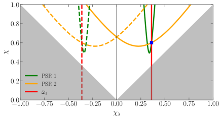
Figure 1: Illustration of the determination of the spin of Sgr A* with measurements of two pulsars in the $\chi$-$\chi_{\lambda}$ plane. The blue square marks the assumed true value of the BH spin. The solid curves show the constraints from two pulsars, while the dashed lines correspond to the $i\leftrightarrow\pi-i$ ambiguity. Shaded region is excluded by the condition $\left|\chi_{\lambda}\right|\leq\chi$.

Figure 1 shows an illustration of using the timing of two pulsars to determine the spin of Sgr A* in the $\chi$-$\chi_{\lambda}$ plane. The system parameters are randomly chosen to avoid the accidental degeneracy which is discussed later. For each pulsar, the measurements of $({\cal X},{\cal W})$ give a hyperbola shown by the solid curve, and the $i\leftrightarrow\pi-i$ ambiguity gives another hyperbola shown by the dashed line. In general, there can exist at most eight different solutions for $(\chi,\chi_{\lambda})$. A rough measurement of any second-order derivatives, for example, the $\ddot{\omega}$ for one of the pulsar, as shown by the vertical red line, or timing of a third pulsar can reduce this degeneracy into two solutions whose $\chi$ has the same value and $\chi_{\lambda}$ has opposite signs.

The methodology described above can be easily extended for combining more pulsars. For each additional pulsar, it provides an independent test of GR as all these curves should intersect at one point within their measurement uncertainties. On the other hand, if one assumes that GR is correct, timing more pulsars can be a unique probe for us to explore and model the (stellar and gas) mass distribution near the GC Merritt et al. (2010); Liu et al. (2012); Hu et al. (2023). As only the leading-order time derivatives and a rough value of a higher-derivative parameter are used, one is expected to obtain a high-precision measurement after a short time observing two pulsars.

Numerical simulation.—To further explore the method introduced above and give a quantitative description of the expected measurement precision in measuring the spin of Sgr A* by timing two pulsars, we perform mock data simulations based on the numerical timing model for pulsar-SMBH systems developed earlier Hu et al. (2023). In this timing model, we numerically integrate the pulsar orbital motion based on the post-Newtonian (PN) equation of motion, $\ddot{\bm{r}}=-GM\hat{\bm{r}}/r^{2}+\ddot{\bm{r}}_{\rm 1PN}+\ddot{\bm{r}}_{\rm SO}+\ddot{\bm{r}}_{\rm Q}$, where $\bm{r}$ is the relative separation pointing from the SMBH to the pulsar, $\ddot{\bm{r}}_{\rm 1PN}$ is the first PN correction, $\ddot{\bm{r}}_{\rm SO}$ and $\ddot{\bm{r}}_{\rm Q}$ are the spin and quadrupole contribution from the central SMBH respectively Barker and O’Connell (1975), $M$ is the mass of the SMBH, $r\equiv|\bm{r}|$, and $\hat{\bm{r}}\equiv\bm{r}/r$. Taking advantage of the PN expansion, we treat the dimensionless spin $\chi$ and the dimensionless quadrupole moment $q$ of the SMBH as independent parameters, which renders a test of the no-hair theorem $q=-\chi^{2}$ for Sgr A* possible Hu et al. (2023). As the mass ratio $m_{\rm PSR}/M\lesssim 10^{-6}$, we treat the pulsar as a test particle in the BH’s spacetime. We take into account the Römer delay, the leading-order Shapiro delay and the Einstein delay in the timing model Shapiro (1964); Blandford and Teukolsky (1976); Damour and Deruelle (1986) and ignore the effects caused by the proper motion of Sgr A* Shklovskii (1970); Kopeikin (1996). More details can be found in Ref. Hu et al. (2023).

The full parameter set, $\bm{\Theta}=\bm{\Theta}_{\rm BH}\cup\bm{\Theta}_{\rm PSR}$, in the timing model for a single pulsar includes the parameters of the SMBH, $\bm{\Theta}_{\rm BH}=\{M,\chi,q,\lambda,\eta\}$, where $\lambda$ and $\eta$ describe the direction of the spin, and the parameters of the pulsar, $\bm{\Theta}_{\rm PSR}=\{P_{b},e,f,i,\omega,N_{0},\nu,\dot{\nu}\}$, where $f$ is the initial orbital phase and $\{N_{0},\nu,\dot{\nu}\}$ relate the pulsar’s rotation number $N$ and pulsar’s proper time $T$ via $N(T)=N_{0}+\nu T+\dot{\nu}T^{2}/2$. We have set the longitude of the ascending node of the pulsar orbit, $\Omega$, to be zero as it is not an observable for timing observation. When combining the timing of two or more pulsars, one should have one set of $\Theta_{\rm PSR}$ for each pulsar while $\Theta_{\rm BH}$ is common for different pulsars. In addition, the difference between the longitudes of the ascending node, $\Delta\Omega=\Omega_{2}-\Omega_{1}$, should also be included in the timing model Ransom et al. (2014). As we can have an overall rotation of the system around the line of sight direction, we fix $\Omega_{1}=0$ in the following discussions and we denote the pulsar with a smaller orbital period as PSR1 or the inner pulsar.

We use the Fisher matrix method for parameter estimation Damour and Deruelle (1986). The log-likelihood function $\mathcal{L}$ in the covariance matrix $C_{\alpha\beta}=\big{(}\partial^{2}\mathcal{L}/\partial\Theta^{\alpha}\partial\Theta^{\beta}\big{)}^{-1}$ is simply the sum from two pulsars, $\mathcal{L}=\mathcal{L}_{1}+\mathcal{L}_{2}$, and

$$\mathcal{L}_{i}=\frac{1}{2\nu_{i}^{2}}\sum_{a=1}^{N^{(i)}_{\rm TOA}}\frac{\left[N^{(i)}_{a}(\bm{\Theta})-N^{(i)}_{a}(\bar{\bm{\Theta}})\right]^{2}}{\left(\sigma^{(i)}_{\rm TOA}\right)^{2}}\,,\ \ i=1,2\,$$ (2)

where $N^{(i)}_{a}(\Theta)=N\Big{(}\Theta;t_{a}^{(i)\,{\rm TOA}}\Big{)}$ is the pulsar rotation number calculated by the timing model corresponding to the $a$-th pulse arrived at $t_{a}^{(i)\,{\rm TOA}}$. $\bar{\bm{\Theta}}$ denotes the true system parameters and $\sigma_{\rm TOA}^{(i)}$ is the timing precision for pulsar $i$. As we do not consider the interaction between the two pulsars, the properties of the Fisher matrix method and the timing model allow one to construct the full Fisher matrix $F\equiv C^{-1}$ though the combination of the Fisher matrices $F_{i}$ of each single pulsar. This simplification is important for combining more pulsars.

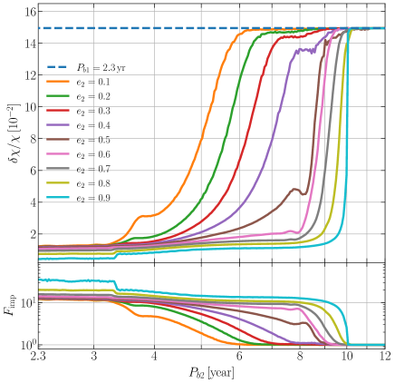
Figure 2: Measurement precision (upper) and improvement factor (lower) for the spin of Sgr A* as functions of the second pulsar’s orbital period ($P_{b2}$) for different orbital eccentricities ($e_{2}$). The solid curves show the measurement precision from combining the timing of two pulsars, while we also show the measurement precision only from the timing of the inner pulsar for comparison (dashed line). The initial orbital position of the second pulsar is set to be at the apocenter, thus one can see at least one pericenter passage for $P_{b2}<10\,{\rm yr}$.

We assume a timing precision $\sigma_{\rm TOA}=1\,{\rm ms}$ and an observation time span $T_{\rm obs}=5\,{\rm yr}$ for both pulsars, which are realistic for future instruments such as the Square Kilometre Array (SKA) and the next-generation Very Large Array (ngVLA) Weltman et al. (2020); Bower et al. (2018). In the upper panel of Fig. 2 we show the measurement precision of the spin of Sgr A* from combining the timing of two pulsars (solid curves) compared to the results obtained from the inner pulsar only (dashed line). Here we fix the orbital period of the inner pulsar to be $P_{b1}=2.3\,{\rm yr}$ and orbital eccentricity $e_{1}=0.8$ while varying the orbital period $P_{b2}$ and eccentricity $e_{2}$ of the second pulsar. The lower panel of this figure shows the improvement factor $F_{\rm imp}=\delta\chi_{\rm single}/\delta\chi_{\rm combine}$. For this case, the inner pulsar with an orbital period $P_{b1}=2.3\,{\rm yr}$ can only constrain $\delta\chi/\chi$ to $\sim 15\%$. Combining a second pulsar even with a large orbital period can provide an improvement factor of $\sim 10$ because of the breaking of the leading-order degeneracy. The improvement factor from combining a second pulsar will be smaller if the inner pulsar has a tighter orbit for which itself can break the leading order degeneracy. Another case study of $P_{b1}=0.5\,{\rm yr}$ shows an improvement factor of $2\sim 3$ when combined with a second pulsar whose orbital period $P_{b2}\lesssim 3\,{\rm yr}$.

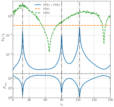
Figure 3: Measurement precision (upper) of the spin parameter as functions of the orbital inclination angle $i_{2}$ of the second pulsar. Two dashed lines show the measurement precision from only one pulsar. The blue curve in the upper panel shows the combined result. The lower panel shows the improvement factor over the inner pulsar. Predictions from Eq. (1) are denoted with vertical lines.

As the second pulsar has a larger orbital period than the inner one, the constraint of the spin from it is in general looser than that from the inner pulsar Psaltis et al. (2016); Zhang and Saha (2017); Bower et al. (2018); Hu et al. (2023). Thus the improvement of the spin measurement by combining two pulsars is mainly caused by the breaking of the leading-order degeneracy. Figure 3 shows an example of the dependence of the degeneracy on the most relevant orbital parameter, the orbital inclination $i$. In this example we set $P_{b1}=2.3\,{\rm yr}$, $e_{1}=0.8$, $P_{b2}=4.2\,{\rm yr}$, and $e_{2}=0.6\,$. The orbital inclination $i_{1}$ of the inner pulsar is fixed to be $60^{\circ}$ and we vary the orbital inclination of the second pulsar, $i_{2}$. One can clearly see that the improvement factor varies over two orders of magnitude and it is not dominated by the second pulsar’s measurement precision.

The simulation results are consistent with the prediction from the analysis we presented before. From Eq. (1), it is obvious that the shape of the hyperbola of each pulsar is controlled by their inclination angles, which determine the leading-order degeneracy. Moreover, from Eq. (1) one can also predict the position of the three degeneracy peaks for the combined results in Fig. 3, where the improvement from combining a second pulsar is the smallest. The central peak at $i=90^{\circ}$ originates from the denominator of the first term in Eq. (1), while the other two peaks are attributed to the situation where two hyperbolas are tangent to each other at the point they intersect. We show the predicted peak positions from Eq. (1) in Fig. 3 with vertical lines.

Pulsars in the GC.—We have shown the large potential of measuring the spin of Sgr A* with two or more pulsars. Compared to the measurement with a single pulsar, the key advantage of the approach we proposed here is that it does not require a pulsar in an extremely compact orbit around Sgr A*. Although several pulsars including a magnetar and a millisecond pulsar have been found in the GC region Eatough et al. (2013); Rea et al. (2013); Lower et al. (2024); Johnston et al. (2006); Deneva et al. (2009); Abbate et al. (2023), none of them are close enough to the Sgr A* for doing the measurement described above. Here we give an estimation of the probability of finding suitable pulsars in future high-frequency radio surveys.

We define two possibilities $P_{1}$ and $P_{2}$ as follows. $P_{1}$ represents the probability of finding the innermost pulsar with an orbital period $P_{b}\leq 0.5\,{\rm yr}$ via future instruments like SKA, which then can be used to measure the spin of Sgr A* by timing itself alone, while $P_{2}$ represents the probability of finding two innermost pulsars both with orbital period $P_{b}\leq 5\,{\rm yr}$. By combining the timing observations of these two pulsars, one may constraint the spin of Sgr A* to $\sim 1\%$ within five years according to our simulations. We assume a simple power-law distribution of pulsars near the Sgr A*, $p(r)\propto r^{-\alpha}$, where $p(r)$ is the probability density of finding a pulsar in a unit volume at a distance $r$ from the Sgr A*. Considering the large uncertainties in the GC pulsar population, the power-law index $\alpha$ can vary largely depending on the detailed models Zhang et al. (2014). Under these assumptions, one can calculate $P_{1}$ and $P_{2}$ via

$$P_{1} = 1-\exp\left[-N_{4}\left(\frac{r_{0.5\,{\rm yr}}}{R_{4}}\right)^{3-\alpha}\right]\,,$$ (3)

$$P_{2} = 1-\left[1+N_{4}\left(\frac{r_{5\,{\rm yr}}}{R_{4}}\right)^{3-\alpha}\right]\exp\left[-N_{4}\left(\frac{r_{5\,{\rm yr}}}{R_{4}}\right)^{3-\alpha}\right]\,,$$ (4)

where $r_{0.5\,{\rm yr}}\sim 100\,{\rm AU}$ and $r_{5\,{\rm yr}}\sim 475\,{\rm AU}$ are the semimajor axes of the pulsar orbits with $P_{b}=0.5\,{\rm yr}$ and $P_{b}=5\,{\rm yr}$ respectively. $N_{4}$ is the expected total number of pulsars that can be observed within $R_{4}=4000\,{\rm AU}$ around Sgr A*. $P_{1}$ and $P_{2}$ for different $\alpha$ and $N_{4}$, motivated from current observations and simulations, are listed in Table 1 Zhang et al. (2014); Torne et al. (2023). In the reasonable parameter space of $\alpha$ and $N_{4}$, one always has $P_{1}\lesssim P_{2}$, indicating that it is more likely to find two pulsars that are suitable for measuring the spin of Sgr A*.

Table 1: $P_{1}$ and $P_{2}$ calculated with Eq. (3) and Eq. (4) for different $\alpha$ and $N_{4}$. In the reasonable parameter space, it is more likely to find two pulsars with orbital periods $P_{b}\leq 5\,{\rm yr}$ rather than a pulsar in a tight orbit that $P_{b}\leq 0.5\,{\rm yr}$.

$\alpha$	$N_{4}$	$P_{1}$	$P_{2}$	$N_{4}$	$P_{1}$	$P_{2}$	$N_{4}$	$P_{1}$	$P_{2}$
$1.6$	$5$	$2.9\%$	$2.7\%$	$10$	$5.7\%$	$9.2\%$	$20$	$11\%$	$27\%$
$2.0$	$5$	$12\%$	$12\%$	$10$	$23\%$	$33\%$	$20$	$40\%$	$69\%$
$2.4$	$5$	$43\%$	$41\%$	$10$	$67\%$	$77\%$	$20$	$89\%$	$98\%$

Discussions.—In this Letter, we proposed to measure the spin of Sgr A* with timing observations of two or more pulsars, which does not require a pulsar with an extremely small orbital period but can still provide similar measurement precision by breaking the leading-order degeneracy of spin parameters. Although the GC pulsar population has a large uncertainty at present, it is expected to find a lot of new pulsars in future high-frequency radio surveys towards the GC and we give a rough estimation of the probability of finding proper systems. It seems that we are more likely to find the systems that are suitable for the procedure proposed here. Even if we can find a pulsar with an orbital period $P_{b}\lesssim 0.5\,{\rm yr}$, combining a proper second pulsar can still provide an improvement factor $\sim 2$ for the SMBH spin measurement.

In this work we have ignored the complex environments near the Sgr A*, which will complicate the measurement Merritt et al. (2010); Liu et al. (2012); Psaltis et al. (2016); Hu et al. (2023). In general, pulsars with larger orbital periods will suffer from more perturbations caused by the mass distributions around Sgr A*, which may even spoil the measurement. It is suggested that one may only use the timing data around the periastron passages and treat each periastron passage incoherently Psaltis et al. (2016). This will enlarge the measurement uncertainty of the spin from timing a single pulsar, where second-order time derivatives are required but hard to measure during the short periastron passage. However, as only the leading-order time derivatives are required in the method we proposed here, it is expected to have a good measurement even only the timing data around the periastron passages are used. On the other hand, by combing the timing observations of more pulsars, one will have the ability to model the mass distribution around Sgr A* that will be of vastly useful for studies of the GC region.