Multiple Greedy Quasi-Newton Methods for Saddle Point Problems

Abstract

This paper introduces the Multiple Greedy Quasi-Newton (MGSR1-SP) method, a novel approach to solving strongly-convex-strongly-concave (SCSC) saddle point problems. Our method enhances the approximation of the squared indefinite Hessian matrix inherent in these problems, significantly improving both stability and efficiency through iterative greedy updates. We provide a thorough theoretical analysis of MGSR1-SP, demonstrating its linear-quadratic convergence rate. Numerical experiments conducted on AUC maximization and adversarial debiasing problems, compared with state-of-the-art algorithms, underscore our method’s enhanced convergence rate. These results affirm the potential of MGSR1-SP to improve performance across a broad spectrum of machine learning applications where efficient and accurate Hessian approximations are crucial.

I Introduction

The saddle point problem is a fundamental formulation in machine learning and optimization and naturally emerges in several applications including game theory [11, 42], robust optimization [9, 54], reinforcement learning [18, 47], AUC maximization [52, 30, 31], fairness-aware machine learning [30, 23], and generative adversarial networks (GANs) [17], etc. In this paper, we consider the following saddle point problem formulated as

$$\min_{{\mathbf{x}}\in\mathbb{R}^{n_{\mathbf{x}}}}\max_{{\mathbf{y}}\in\mathbb{R}^{n_{\mathbf{y}}}}f({\mathbf{x}},{\mathbf{y}}),$$ (1)

where $f({\mathbf{x}},{\mathbf{y}})$ is smooth, strongly-convex in ${\mathbf{x}}$, and strongly-concave in ${\mathbf{y}}$. The objective is to find the saddle point $({\mathbf{x}}^{*},{\mathbf{y}}^{*})$ such that:

$$f({\mathbf{x}}^{*},{\mathbf{y}})\leq f({\mathbf{x}}^{*},{\mathbf{y}}^{*})\leq f({\mathbf{x}},{\mathbf{y}}^{*})$$

for all ${\mathbf{x}}\in{\mathbb{R}}^{n_{\mathbf{x}}},{\mathbf{y}}\in{\mathbb{R}}^{n_{\mathbf{y}}}$.

Several first-order optimization techniques have been developed to solve saddle point problems, achieving a linear convergence rate with an iteration complexity of ${\mathcal{O}}(1/\epsilon)$. These include the extragradient (EG) method [25, 51], the optimistic gradient descent ascent (OGDA) method [10, 40], the proximal point method [43], the mirror-prox method [24], and the dual extrapolation method [37]. Their stochastic variants have also been explored in large-scale settings [3, 7, 34, 35, 38, 50].

Second-order methods enhance iteration complexity compared to first-order methods but often require higher computational demands. The cubic regularized Newton (CRN) method, which achieves quadratic local convergence, requires the computation of the exact Hessian matrix and solving of cubic variational inequality sub-problems [19]. Other adaptations, such as the Newton proximal extragradient [16, 49], the mirror-prox algorithm [4], and the second-order optimistic method [21], incorporate line searches for step size optimization. Conversely, methods such as those proposed in [2, 29, 32], avoid such complexities by omitting line searches and following a more streamlined approach akin to the CRN method, balancing efficiency and effectiveness in various optimization settings. Recently,

Quasi-Newton methods approximate the Hessian matrix and its inverse rather than directly computing them, utilizing iterative updates to significantly reduce per-iteration costs. Notable quasi-Newton formulas for minimization include the BFGS [36, 20, 26], DFP [14, 15], and PSB [41]. Recent advancements include [44, 45, 46, 33] have introduced greedy, random and higher rank variants that achieve superlinear convergence. Despite their success in minimization problems, quasi-Newton methods are less commonly applied to saddle point problems. Research has explored proximal quasi-Newton methods for monotone variational inequalities [6, 5, 8]. Recent developments [1, 13, 30, 31] have introduced new quasi-Newton methods, although these adaptations may lack stability.

In this paper, we propose a multiple greedy quasi-Newton method for SCSC saddle point problems, which leverages the approximation of the squared Hessian matrix with multiple greedy quasi-Newton updates per iteration. We rigorously establish a linear to quadratic convergence rate for our algorithm. Through numerical experiments on popular machine learning problems, including AUC maximization and adversarial debiasing, we demonstrate the superior performance of our algorithm compared to state-of-the-art alternatives. The paper is organized as follows:

Paper Organization In Section II, we clarify the notations and provide assumptions and preliminaries of this paper. In Section III, we introduce a framework for saddle point problems and propose our MGSR1-SP algorithm with theoretical convergence guarantee. In Section IV, we validate our algorithm on AUC maximization and Adverasial Debiasing problems.

II Notation and Preliminaries

We use $\|\cdot\|$ to denote the spectral norm and the Euclidean norm of a matrix and a vector, respectively. The standard basis in ${\mathbb{R}}^{d}$ is denoted by $\{\mathbf{e}_{1},\dots,\mathbf{e}_{d}\}$. The identity matrix is represented as ${\mathbf{I}}$, and the trace of any square matrix is represented by $\text{tr}(\cdot)$. We use ${\mathbb{S}}_{++}^{d}$ to represent the set of positive definite matrices. For two positive definite matrices ${\mathbf{Q}}\in{\mathbb{S}}_{++}^{d}$ and ${\mathbf{H}}\in{\mathbb{S}}_{++}^{d}$, their inner product is defined as $\langle{\mathbf{Q}},{\mathbf{H}}\rangle=\text{tr}({\mathbf{Q}}{\mathbf{H}})$. We denote ${\mathbf{Q}}\succeq{\mathbf{H}}$ if ${\mathbf{G}}-{\mathbf{H}}\succeq 0$. Referring to the objective function in equation (1), let $d=d_{\mathbf{x}}+d_{\mathbf{y}}$ represent the full dimension. The gradient ${\mathbf{g}}({\mathbf{x}}_{k},{\mathbf{y}}_{k})$ and Hessian matrix $\tilde{{\mathbf{H}}}({\mathbf{x}}_{k},{\mathbf{y}}_{k})$ of function $f$ at the $k$-th iteration at $({\mathbf{x}}_{k},{\mathbf{y}}_{k})$ are denoted as ${\mathbf{g}}_{k}\in\mathbb{R}^{d}$ and $\tilde{{\mathbf{H}}}_{k}\in\mathbb{R}^{d\times d}$ respectively. We also use ${\mathbf{H}}_{{\mathbf{x}}{\mathbf{x}}},{\mathbf{H}}_{{\mathbf{x}}{\mathbf{y}}}$ and ${\mathbf{H}}_{{\mathbf{y}}{\mathbf{y}}}$ to denote the sub-matrices.

Suppose that the objective function in Eq. (1) satisfies the following assumptions:

Assumption 1.

The objective function $f(\mathbf{x},\mathbf{y})$ is twice differentiable with $L_{1}$-Lipschitz gradient and $L_{2}$-Lipschitz Hessian, i.e.,

$$\|\mathbf{g}({\mathbf{x}},{\mathbf{y}})-{\mathbf{g}}({\mathbf{x}}^{\prime},{\mathbf{y}}^{\prime})\|\leq L_{1}\bigg{\|}\begin{bmatrix}{\mathbf{x}}-{\mathbf{x}}^{\prime}\\ {\mathbf{y}}-{\mathbf{y}}^{\prime}\end{bmatrix}\bigg{\|}$$

and

$$\|\tilde{{\mathbf{H}}}({\mathbf{x}},{\mathbf{y}})-\tilde{{\mathbf{H}}}({\mathbf{x}}^{\prime},{\mathbf{y}}^{\prime})\|\leq L_{2}\bigg{\|}\begin{bmatrix}{\mathbf{x}}-{\mathbf{x}}^{\prime}\\ {\mathbf{y}}-{\mathbf{y}}^{\prime}\end{bmatrix}\bigg{\|}$$

for any $[{\mathbf{x}};{\mathbf{y}}]^{\top}\in{\mathbb{R}}^{d}\text{ and }[{\mathbf{x}}^{\prime};{\mathbf{y}}^{\prime}]^{\top}\in{\mathbb{R}}^{d}$.

Assumption 2.

The objective function $f(\mathbf{x},\mathbf{y})$ is $\mu$-strongly-convex in $\mathbf{x}$ and $\mu$-strongly-concave in $\mathbf{y}$, i.e.,

$$\tilde{{\mathbf{H}}}_{{\mathbf{x}}{\mathbf{x}}}\succeq\mu{\mathbf{I}}$$

and

$$\tilde{{\mathbf{H}}}_{{\mathbf{y}}{\mathbf{y}}}\preceq-\mu{\mathbf{I}}$$

for any $[{\mathbf{x}};{\mathbf{y}}]^{\top}\in{\mathbb{R}}^{d}$. Additionally, the condition number of the objective function is defined as $\kappa=L_{1}/\mu$.

Note that the Hessian matrix $\tilde{\mathbf{H}}(\mathbf{x},\mathbf{y})$ in saddle point problems in Eq. (1) is usually indefinite. However, the following lemma derived a crucial property of the squared Hessian matrix, guaranteeing positive definiteness.

Lemma 1.

Define ${\mathbf{H}}({\mathbf{x}},{\mathbf{y}})=\tilde{{\mathbf{H}}}({\mathbf{x}},{\mathbf{y}})^{2}$. Under Assumption 1 and Assumption 2, we have $\mu^{2}\mathbf{I}\preceq{\mathbf{H}}({\mathbf{x}},{\mathbf{y}})\preceq L_{1}^{2}{\mathbf{I}}$ for any $[{\mathbf{x}};{\mathbf{y}}]^{\top}\in{\mathbb{R}}^{d}$.

III Algorithm and Theoretical Analysis

In this section, we first present a framework for saddle point problems. We then review the fundamentals of quasi-Newton methods, emphasizing the greedy variant from [44]. Finally, We then introduce our MGSR1-SP algorithm and provide its convergence guarantee.

III-A A Quasi-Newton Framework for Saddle Point Problems

The standard update formula for Newton’s method is expressed as

$$\begin{bmatrix}{\mathbf{x}}_{k+1}\\ {\mathbf{y}}_{k+1}\end{bmatrix}=\begin{bmatrix}{\mathbf{x}}_{k}\\ {\mathbf{y}}_{k}\end{bmatrix}-\tilde{{\mathbf{H}}}_{k}^{-1}{\mathbf{g}}_{k},$$

which exhibits quadratic local convergence. However, this method incurs a computational complexity of ${\mathcal{O}}(d^{3})$ per iteration for the inverse Hessian matrix. In the realm of convex minimization, quasi-Newton methods such as BFGS, SR1, and their variations focus on approximating the Hessian matrix to reduce computational demands to ${\mathcal{O}}(d^{2})$ per iteration. Nonetheless, these methods presuppose a positive definite Hessian, which is unsuitable for saddle point problems as described in Eq. (1) due to the inherent indefiniteness of $\tilde{{\mathbf{H}}}({\mathbf{x}},{\mathbf{y}})$. To address this challenge, [31] reformulated the Newton’s method as

$$\begin{bmatrix}{\mathbf{x}}_{k+1}\\ {\mathbf{y}}_{k+1}\end{bmatrix}=\begin{bmatrix}{\mathbf{x}}_{k}\\ {\mathbf{y}}_{k}\end{bmatrix}-[(\tilde{{\mathbf{H}}}_{k})^{2}]^{-1}\tilde{{\mathbf{H}}}_{k}{\mathbf{g}}_{k}=\begin{bmatrix}{\mathbf{x}}_{k}\\ {\mathbf{y}}_{k}\end{bmatrix}-{\mathbf{H}}_{k}^{-1}\tilde{{\mathbf{H}}}_{k}{\mathbf{g}}_{k}.$$ (2)

where ${\mathbf{H}}_{k}=\tilde{{\mathbf{H}}}_{k}^{2}$ is the auxiliary matrix defined in Lemma 1, which is guaranteed to be positive definite. Consequently, the update rule for Newton’s method can be reformulated as

$$\begin{bmatrix}{\mathbf{x}}_{k+1}\\ {\mathbf{y}}_{k+1}\end{bmatrix} =\begin{bmatrix}{\mathbf{x}}_{k}\\ {\mathbf{y}}_{k}\end{bmatrix}-{\mathbf{Q}}_{k}^{-1}\tilde{{\mathbf{H}}}_{k}{\mathbf{g}}_{k},$$ (3)

where ${\mathbf{Q}}_{k}^{-1}\in{\mathbb{S}}_{++}^{d}$ is an approximated inverse matrix of ${\mathbf{H}}_{k}^{-1}$. We will introduce the techniques to construct ${\mathbf{Q}}_{k}$ and its inverse in the next section. Note that the update rule (3) does not necessarily require the explicit construction of Hessian matrix, which can be computed efficiently through Hessian-Vector Product (HVP) [39, 48].

III-B Greedy Quasi-Newton Methods

Quasi-Newton methods are developed to circumvent some of the computational inefficiencies associated with the classical Newton’s method [27, 44, 31, 53, 28, 46, 22]. Among these, the Broyden family update is the most widely used in literature. Given two symmetric positive definite matrices ${\mathbf{H}},{\mathbf{Q}}\in{\mathbb{S}}^{d}_{++}$ and a vector ${\mathbf{u}}\in{\mathbb{R}}^{d}$, satisfying that ${\mathbf{Q}}\succeq{\mathbf{H}}$ and ${\mathbf{Q}}{\mathbf{u}}\neq{\mathbf{A}}{\mathbf{u}}$, the Broyden family update is given by

$$\text{Broyd}_{\tau}({\mathbf{Q}},{\mathbf{H}},{\mathbf{u}})=\tau\text{DFP}({\mathbf{Q}}, {\mathbf{H}},{\mathbf{u}})$$

$$+(1-\tau)\text{SR1}({\mathbf{Q}},{\mathbf{H}},{\mathbf{u}}),$$

which is proved to be a convex combination [44]. The SR1 update is given by

$$\text{SR1}({\mathbf{Q}},{\mathbf{H}},{\mathbf{u}})={\mathbf{Q}}-\frac{({\mathbf{Q}}-{\mathbf{H}}){\mathbf{u}}{\mathbf{u}}^{\top}({\mathbf{Q}}-{\mathbf{H}})}{{\mathbf{u}}^{\top}({\mathbf{Q}}-{\mathbf{H}}){\mathbf{u}}},$$

which leverages a rank-one modification to adjust ${\mathbf{Q}}$ based on the discrepancy between ${\mathbf{Q}}$ and ${\mathbf{H}}$. On the other hand, the DFP update incorporates both current and previous curvature information into the approximation:

$$\text{DFP}({\mathbf{Q}},{\mathbf{H}},{\mathbf{u}})={\mathbf{Q}}- \frac{{\mathbf{H}}{\mathbf{u}}{\mathbf{u}}^{\top}{\mathbf{Q}}+{\mathbf{Q}}{\mathbf{u}}{\mathbf{u}}^{\top}{\mathbf{H}}}{{\mathbf{u}}^{\top}{\mathbf{H}}{\mathbf{u}}}$$

$$+\bigg{(}1+\frac{{\mathbf{u}}^{\top}{\mathbf{Q}}{\mathbf{u}}}{{\mathbf{u}}^{\top}{\mathbf{H}}{\mathbf{u}}}\bigg{)}\frac{{\mathbf{H}}{\mathbf{u}}{\mathbf{u}}^{\top}{\mathbf{H}}}{{\mathbf{u}}^{\top}{\mathbf{H}}{\mathbf{u}}}.$$

The parameter $\tau\in[0,1]$ determines the specific type of Quasi-Newton update applied. Specifically, setting $\tau=\frac{{\mathbf{u}}^{\top}{\mathbf{H}}{\mathbf{u}}}{{\mathbf{u}}^{\top}{\mathbf{Q}}{\mathbf{u}}}$ leads to the well-known Broyden-Fletcher-Goldfarb-Shanno (BFGS) update formulated as

$$\text{BFGS}({\mathbf{Q}},{\mathbf{H}},{\mathbf{u}})={\mathbf{Q}}-\frac{{\mathbf{Q}}{\mathbf{u}}{\mathbf{u}}^{\top}{\mathbf{Q}}}{{\mathbf{u}}^{\top}{\mathbf{Q}}{\mathbf{u}}}+\frac{{\mathbf{H}}{\mathbf{u}}{\mathbf{u}}^{\top}{\mathbf{H}}}{{\mathbf{u}}^{\top}{\mathbf{H}}{\mathbf{u}}}.$$

Greedy Quasi-Newton methods were proposed to achieve better convergence rates than classical Quasi-Newton methods, with a contraction factor that depends on the square of the iteration counter [44]. Specifically, for a given target matrix ${\mathbf{H}}\in{\mathbb{S}}_{++}^{d}$ and an approximator ${\mathbf{Q}}\succeq{\mathbf{H}}$, the greedily selected vector ${\mathbf{u}}$ is determined as follows:

$${\mathbf{u}}_{\mathbf{H}}({\mathbf{Q}})=\operatorname*{arg\,max}_{{\mathbf{u}}\in\{{\mathbf{e}}_{1},\ldots,{\mathbf{e}}_{n}\}}\frac{{\mathbf{u}}^{\top}{\mathbf{Q}}{\mathbf{u}}}{{\mathbf{u}}^{\top}{\mathbf{H}}{\mathbf{u}}},$$

where ${\mathbf{e}}_{i}$ represents the basis vector. Define the greedy Broyden family update as follows:

$$\text{gBroyd}_{\tau}({\mathbf{Q}},{\mathbf{H}})\overset{\rm{def}}{=}\text{Broyd}_{\tau}({\mathbf{Q}},{\mathbf{H}},{\mathbf{u}}_{\mathbf{H}}({\mathbf{Q}})).$$

Specifically, if $\tau=0$, the update is greedy SR1 update defined as

$$\text{gSR1}({\mathbf{Q}},{\mathbf{H}})\overset{\rm{def}}{=}\text{gSR1}({\mathbf{Q}},{\mathbf{H}},{\mathbf{u}}_{\mathbf{H}}({\mathbf{Q}})).$$ (4)

The following lemma demonstrates that the greedy SR1 update reduces the rank of ${\mathbf{Q}}-{\mathbf{H}}$ at each iteration. Therefore, with at most $d$ iterations, the gSR1 update will accurately recover the Hessian matrix.

Theorem 1 ([44], Theorem 3.5).

Suppose that for each $k\geq 0$, we choose ${\mathbf{u}}_{k}={\mathbf{u}}_{\mathbf{H}}({\mathbf{Q}}_{k})$ and $\tau=0$, then ${\mathbf{Q}}_{k}={\mathbf{H}}$ for some $0\leq k\leq d$.

In quadratic optimization, the Hessian matrix remains constant, which means the approximator ${\mathbf{Q}}$ converges to ${\mathbf{H}}$ with each iteration. For more general problems, we define the multiple $\text{gBroyd}_{\tau}^{n}$ as a series of nested $\text{gBroyd}_{\tau}$ updates [12] such that

$${\mathbf{Q}}_{i+1}\leftarrow\text{gBroyd}_{\tau}^{n}({\mathbf{Q}}_{i},{\mathbf{H}}),\quad i=0,\dots,n-1,$$

where $n$ is a non-negative integer representing the counts of greedy Broyden family updates performed in each iteration. Specifically, the multiple greedy SR1 update denoted as $\text{gSR1}^{n}$ is performed as follows:

$${\mathbf{Q}}_{i+1}\leftarrow\text{gSR1}({\mathbf{Q}},{\mathbf{H}}),\quad i=0,\dots,n-1.$$ (5)

III-C MGSR1-SP Algorithm and Convergence Analysis

In this section, we introduce the Multiple Greedy Rank-1 (MGSR1-SP) algorithm for saddle point problems satisfying Assumption 1 and Assumption 2, which is outlined in Algorithm 1. The MGSR1-SP algorithm builds upon the framework in Section III-A and adopts the multiple greedy SR1 updates specified in Eq. (5).

Algorithm 1 MGSR1-SP

1:Initialization: ${\mathbf{z}}_{0}$, ${\mathbf{Q}}_{0}$, stepsize $\alpha$, $M$, and $n\geq 0$.

2:for k in $0,\dots,N$ do

3:     Compute ${\mathbf{g}}_{k}$

4:     Update ${\mathbf{z}}_{k+1}\leftarrow{\mathbf{z}}_{k}-\alpha\cdot{\mathbf{Q}}_{k}^{-1}\tilde{{\mathbf{H}}}_{k}{\mathbf{g}}_{k}\ \text{(HVP)}$

5:     Perform $\text{gSR1}^{n}$ updates: $\tilde{{\mathbf{Q}}}_{k}=\text{gSR1}^{n}({\mathbf{Q}}_{k},{\mathbf{H}}_{k}).$

6:     Compute $r_{k}=\bigg{\|}\begin{bmatrix}{\mathbf{x}}_{k+1}-{\mathbf{x}}_{k}\\ {\mathbf{y}}_{k+1}-{\mathbf{y}}_{k}\end{bmatrix}\bigg{\|}$

7:     Correct $\tilde{{\mathbf{Q}}}_{k+1}\leftarrow(1+Mr_{k})\tilde{{\mathbf{Q}}}_{k}$

8:     Compute ${\mathbf{Q}}_{k+1}=\text{gSR1}(\tilde{{\mathbf{Q}}}_{k+1},{\mathbf{H}}_{k+1}))$

9:end for

Lemma 2 (Modified from [44]).

If, for some $\eta\geq 1$, and two positive definite matrix ${\mathbf{H}},{\mathbf{Q}}\in{\mathbb{S}}_{++}^{d}$, we have

$${\mathbf{H}}\preceq{\mathbf{Q}}\preceq\eta{\mathbf{H}},$$

then using greedy SR1 update (4), we have

$${\mathbf{H}}\preceq\text{gSR1$({\mathbf{Q}},{\mathbf{H}})$}\preceq\eta{\mathbf{H}}.$$

Lemma 3 (Modified from [30]).

Let $[{\mathbf{x}}_{k};{\mathbf{y}}_{k}]^{\top}\in{\mathbb{R}}^{d}\text{ and }[{\mathbf{x}}_{k+1};{\mathbf{y}}_{k+1}]^{\top}\in{\mathbb{R}}^{d}$ with squared Hessian matrix ${\mathbf{H}}_{k},{\mathbf{H}}_{k+1}\in{\mathbb{S}}_{++}^{d}$ defined in Lemma 1, respectively. For some $\eta\geq 1$ and let ${\mathbf{Q}}_{k}\in{\mathbb{S}}_{++}^{d}$ be a positive definite matrix such that

$${\mathbf{H}}_{k}\preceq{\mathbf{Q}}_{k}\preceq\eta{\mathbf{H}}_{k},$$

we have

$${\mathbf{H}}_{k+1}\preceq\text{gSR1}(\tilde{{\mathbf{Q}}}_{k+1},{\mathbf{H}}_{k+1})\preceq(1+Mr_{k})^{2}\eta{\mathbf{H}}_{k+1}$$

where $\tilde{{\mathbf{Q}}}_{k+1}=(1+Mr_{k}){\mathbf{Q}}_{k}$, $r_{k}=\bigg{\|}\begin{bmatrix}{\mathbf{x}}_{k+1}-{\mathbf{x}}_{k}\\ {\mathbf{y}}_{k+1}-{\mathbf{y}}_{k}\end{bmatrix}\bigg{\|}$ and $M=\frac{2\kappa^{2}L_{2}}{L_{1}}$.

Given upon this, define the convergence measure as

$$\lambda_{k}=\lambda({\mathbf{x}}_{k},{\mathbf{y}}_{k})=\|{\mathbf{g}}({\mathbf{x}}_{k},{\mathbf{y}}_{k})\|_{2},$$ (6)

we establish a linear to quadratic convergence rate for our MGSR1-SP algorithm in the following theorem.

Theorem 2.

Using Algorithm 1, suppose we have ${\mathbf{H}}_{k}\preceq{\mathbf{Q}}_{k}\preceq\eta_{k}{\mathbf{H}}_{k}$ for some $\eta_{k}\geq 1$, and let $\beta=\frac{L_{2}}{2\mu^{2}}$, then we have

$$\lambda_{k+1} \leq\bigg{(}1-\frac{1}{\eta_{k}}\bigg{)}\lambda_{k}+\beta\lambda_{k}^{2}.$$

Proof Sketch. Suppose ${\mathbf{H}}_{k}\preceq{\mathbf{Q}}_{k}\preceq\eta_{k}{\mathbf{H}}_{k}$ holds, with Lemma 2, the multiple greedy SR1 update also satisfies ${\mathbf{H}}_{k}\preceq\text{gSR1}^{n}({\mathbf{Q}}_{k},{\mathbf{H}}_{k})\preceq\eta{\mathbf{H}}_{k}$, hence, following Lemma 3, we have ${\mathbf{H}}_{k+1}\preceq{\mathbf{Q}}_{k+1}\preceq(1+Mr_{k})^{2}\eta_{k}{\mathbf{H}}_{k+1}=\eta_{k+1}{\mathbf{H}}_{k+1}$. The rest follows Lemma 3.14 in [30]. ∎

IV Numerical Experiments

In this section, we demonstrate the efficiency of our algorithm using two popular machine learning tasks: AUC maximization and adversarial debiasing. The experiments were conducted on a Macbook Air with M2 chip.

IV-A AUC Maximization

In machine learning, the Area Under the ROC Curve (AUC) is a key metric that evaluates classifier performance in binary classification, particularly useful with imbalanced data. The problem can be formulated as follows:

$$f({\mathbf{x}},y):=\frac{1}{m}\sum_{i=1}^{m}f_{i}({\mathbf{x}},y)+\frac{\lambda}{2}\|{\mathbf{x}}\|^{2}-p(1-p)y^{2},$$

where ${\mathbf{x}}=[{\mathbf{w}};u;v]^{\top}\in{\mathbb{R}}^{n_{\mathbf{x}}},y\in{\mathbb{R}}$, $\lambda$ is the regularization parameter and $p$ denotes the proportion of positive instances in the dataset. The function $f_{i}({\mathbf{x}},y)$ is defined as:

$$f_{i}({\mathbf{x}},y)= (1-p)\big{(}({\mathbf{w}}^{\top}{\mathbf{a}}_{j}-u)^{2}-2(1+y){\mathbf{w}}^{\top}{\mathbf{a}}_{j}\big{)}{\mathbf{I}}_{b_{j}=1}$$

$$+p\big{(}({\mathbf{w}}^{\top}{\mathbf{a}}_{j}-v)^{2}+2(1+y){\mathbf{w}}^{\top}{\mathbf{a}}_{j}\big{)}{\mathbf{I}}_{b_{j}=-1},$$

where ${\mathbf{a}}_{i}\in\mathbb{R}^{n_{\mathbf{x}}-2}$ are features and $b_{i}\in\{+1,-1\}$ is the label.

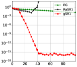
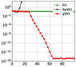
(a) a9a, #iter	(b) w8a, #iter
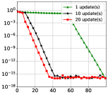
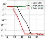
(c) a9a, #iter	(d) w8a, #iter

Figure 1: Numerical results for AUC Maximization task. The y-axis denotes the gradient norm $\|\nabla f({\mathbf{x}},y)\|_{2}$ and x-axis denotes the number of iterations. Top two figures compares Extragradient, RandomSR1 and MGSR1-SP(‘gSR1’) with 20 rounds update on ‘a9a’ and ‘w8a’ dataset. Bottom two figures compare MGSR1-SP(‘gSR1’) with different number of updates per iteration.

IV-B Adversarial Debiasing

Adversarial debiasing is a prominent method used to enhance equity in AI by integrating adversarial techniques to mitigate biases within machine learning algorithms. Given a dataset $\{{\mathbf{a}}_{i},b_{i},c_{i}\}_{i=1}^{m}$, where ${\mathbf{a}}_{i}$ represents input variables, $b_{i}\in\mathbb{R}$ is the output, and $c_{i}\in\mathbb{R}$ is the protected variable, the objective is to reduce bias, which can be formulated as:

$$f({\mathbf{x}},y)=\frac{1}{m}\sum_{i=1}^{m}f_{i}({\mathbf{x}},y)+\lambda\|{\mathbf{x}}\|^{2}-\gamma y^{2},$$

where $\lambda,\gamma$ are regularization parameters. The function $f_{i}({\mathbf{x}},y)$ is defined as

$$f_{i}({\mathbf{x}},y)= \log\big{(}1+\exp\big{(}-b_{j}({\mathbf{a}}_{j})^{\top}{\mathbf{x}}\big{)}\big{)}$$

$$-\beta\log\big{(}1+\exp\big{(}-c_{j}({\mathbf{a}}_{j})^{\top}{\mathbf{x}}y\big{)}\big{)},$$

with $\beta$ also serving as a regularization parameter.

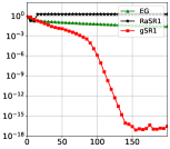
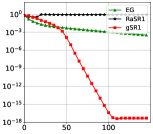
(a) adult, #iter	(b) law, #iter
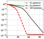
(c) adult, #iter	(d) law, #iter

Figure 2: Numerical results for Adversarial Debiasing. The y-axis denotes the gradient norm $\|\nabla f({\mathbf{x}},y)\|_{2}$ and x-axis denotes the number of iterations. Top two figures compares Extragradient, RandomSR1 and MGSR1-SP(‘gSR1’) with 20 rounds update on ‘a9a’ and ‘w8a’ dataset. Bottom two figures compare MGSR1-SP(‘gSR1’) with different number of updates per iteration.

IV-C Results Analysis

We evaluated the performance of our MGSR1-SP algorithm against two baselines: Random SR1, where vectors $\mathbf{u}\in\mathbb{R}^{d}$ are drawn from a normal distribution $\mathcal{N}(0,1)$, and the ExtraGradient algorithm for saddle point problems.

For AUC maximization, the experiments were conducted on the ‘a9a’ dataset ($n_{\mathbf{x}}=125,n_{\mathbf{y}}=1,N=32651$) and the ‘w8a’ dataset ($n_{\mathbf{x}}=302,n_{\mathbf{y}}=1,N=45546$). The results are shown in Figure 1. Note that the Hessian AUC maximization is invariant ($L_{2}=0$), indicating a linear convergence rate 2. Our MGSR1-SP algorithm demonstrated a faster convergence rate compared to the ExtraGradient algorithm. Moreover, it offered more stable Hessian approximations than the random SR1 update, particularly as the number of update rounds increased.

For adversarial debiasing, the experiments were conducted using the ‘adult’ dataset ($n_{\mathbf{x}}=122,n_{\mathbf{y}}=1,N=32651$) and the ‘law school’ dataset ($n_{\mathbf{x}}=379,n_{\mathbf{y}}=1,N=20427$). The results, shown in Figure 2, indicated that our algorithm achieved a linear-quadratic convergence rate. Our method outperformed both EG and Random SR1 in terms of iterations required, with significant performance improvements as updates increased.

V Conclusion

In this paper, we propose a Multiple Greedy Quasi-Newton (MGSR1-SP) method for strongly-convex-strongly-concave (SCSC) saddle point problems. This algorithm approximates the squared indefinite Hessian matrix, enhancing accuracy and efficiency through a series of iterative greedy quasi-Newton updates. We rigorously established the theoretical results of the MGSR1-SP algorithm, demonstrating its linear-quadratic convergence rates. Furthermore, we conducted numerical experiments against state-of-the-art methods including the EG and Random SR1 algorithms, on two popular machine learning applications. The results clearly show that our method not only converges faster but also provides a more accurate and stable estimation of the inverse Hessian matrix.

For future work, several promising directions can be explored. These include adapting the MGSR1-SP framework to stochastic settings. Additionally, the development of limited memory quasi-Newton methods could make our approach feasible for large-scale problems, where computational resources and memory usage are significant constraints. Another area of potential exploration is the integration of adaptive step-size mechanisms to enhance effectiveness. Lastly, extending our method to handle non-convex saddle point problems with regularization could broaden its applicability to a wider range of machine learning problems.

References

- Abdi and Shakeri [2019] Fatemeh Abdi and Fatemeh Shakeri. A globally convergent bfgs method for pseudo-monotone variational inequality problems. Optimization Methods and Software, 34(1):25–36, 2019.
- Adil et al. [2022] Deeksha Adil, Brian Bullins, Arun Jambulapati, and Sushant Sachdeva. Optimal methods for higher-order smooth monotone variational inequalities. arXiv preprint arXiv:2205.06167, 2022.
- Alacaoglu and Malitsky [2022] Ahmet Alacaoglu and Yura Malitsky. Stochastic variance reduction for variational inequality methods. In Conference on Learning Theory, pages 778–816. PMLR, 2022.
- Bullins and Lai [2022] Brian Bullins and Kevin A Lai. Higher-order methods for convex-concave min-max optimization and monotone variational inequalities. SIAM Journal on Optimization, 32(3):2208–2229, 2022.
- Burke and Qian [1999] James V Burke and Maijian Qian. A variable metric proximal point algorithm for monotone operators. SIAM Journal on Control and Optimization, 37(2):353–375, 1999.
- Burke and Qian [2000] James V Burke and Maijian Qian. On the superlinear convergence of the variable metric proximal point algorithm using broyden and bfgs matrix secant updating. Mathematical Programming, 88:157–181, 2000.
- Chavdarova et al. [2019] Tatjana Chavdarova, Gauthier Gidel, François Fleuret, and Simon Lacoste-Julien. Reducing noise in gan training with variance reduced extragradient. Advances in Neural Information Processing Systems, 32, 2019.
- Chen and Fukushima [1999] Xiaojun Chen and Masao Fukushima. Proximal quasi-newton methods for nondifferentiable convex optimization. Mathematical Programming, 85:313–334, 1999.
- Chen and Kelley [2024] Xiaojun Chen and Carl Kelley. Min-max optimization for robust nonlinear least squares problems. arXiv preprint arXiv:2402.12679, 2024.
- Daskalakis et al. [2017] Constantinos Daskalakis, Andrew Ilyas, Vasilis Syrgkanis, and Haoyang Zeng. Training gans with optimism. arXiv preprint arXiv:1711.00141, 2017.
- Du and Pardalos [1995] Ding-Zhu Du and Panos M Pardalos. Minimax and applications, volume 4. Springer Science & Business Media, 1995.
- Du and You [2024] Yubo Du and Keyou You. Distributed adaptive greedy quasi-newton methods with explicit non-asymptotic convergence bounds. Automatica, 165:111629, 2024.
- Essid et al. [2023] Montacer Essid, Esteban G Tabak, and Giulio Trigila. An implicit gradient-descent procedure for minimax problems. Mathematical Methods of Operations Research, 97(1):57–89, 2023.
- Fletcher [1970] Roger Fletcher. A new approach to variable metric algorithms. The computer journal, 13(3):317–322, 1970.
- Fletcher and Powell [1963] Roger Fletcher and Michael JD Powell. A rapidly convergent descent method for minimization. The computer journal, 6(2):163–168, 1963.
- Gonçalves et al. [2020] Max LN Gonçalves, Jefferson G Melo, and Renato DC Monteiro. On the iteration-complexity of a non-euclidean hybrid proximal extragradient framework and of a proximal admm. Optimization, 69(4):847–873, 2020.
- Goodfellow et al. [2020] Ian Goodfellow, Jean Pouget-Abadie, Mehdi Mirza, Bing Xu, David Warde-Farley, Sherjil Ozair, Aaron Courville, and Yoshua Bengio. Generative adversarial networks. Communications of the ACM, 63(11):139–144, 2020.
- He et al. [2023] Jiafan He, Heyang Zhao, Dongruo Zhou, and Quanquan Gu. Nearly minimax optimal reinforcement learning for linear markov decision processes. In International Conference on Machine Learning, pages 12790–12822. PMLR, 2023.
- Huang et al. [2022] Kevin Huang, Junyu Zhang, and Shuzhong Zhang. Cubic regularized newton method for the saddle point models: A global and local convergence analysis. Journal of Scientific Computing, 91(2):60, 2022.
- Javad Ebadi et al. [2023] Mohammad Javad Ebadi, Amin Fahs, Hassane Fahs, and Razieh Dehghani. Competitive secant (bfgs) methods based on modified secant relations for unconstrained optimization. Optimization, 72(7):1691–1706, 2023.
- Jiang and Mokhtari [2022] Ruichen Jiang and Aryan Mokhtari. Generalized optimistic methods for convex-concave saddle point problems. arXiv preprint arXiv:2202.09674, 2022.
- Jin and Mokhtari [2023] Qiujiang Jin and Aryan Mokhtari. Non-asymptotic superlinear convergence of standard quasi-newton methods. Mathematical Programming, 200(1):425–473, 2023.
- Jin and Lai [2023] Yulu Jin and Lifeng Lai. Fairness-aware regression robust to adversarial attacks. IEEE Transactions on Signal Processing, 2023.
- Juditsky et al. [2011] Anatoli Juditsky, Arkadi Nemirovski, and Claire Tauvel. Solving variational inequalities with stochastic mirror-prox algorithm. Stochastic Systems, 1(1):17–58, 2011.
- [25] GM Korpelevich. An extragradient method for finding saddle points and for other problems, ekonomika i matematicheskie metody, 12 (1976), 747–756. Search in.
- Lai et al. [2023] Kin Keung Lai, Shashi Kant Mishra, Ravina Sharma, Manjari Sharma, and Bhagwat Ram. A modified q-bfgs algorithm for unconstrained optimization. Mathematics, 11(6):1420, 2023.
- Lee et al. [2018] Ching-pei Lee, Cong Han Lim, and Stephen J Wright. A distributed quasi-newton algorithm for empirical risk minimization with nonsmooth regularization. In Proceedings of the 24th ACM SIGKDD international conference on knowledge discovery & data mining, pages 1646–1655, 2018.
- Lin et al. [2022] Dachao Lin, Haishan Ye, and Zhihua Zhang. Explicit convergence rates of greedy and random quasi-newton methods. Journal of Machine Learning Research, 23(162):1–40, 2022.
- Lin and Jordan [2024] Tianyi Lin and Michael I Jordan. Perseus: A simple and optimal high-order method for variational inequalities. Mathematical Programming, pages 1–42, 2024.
- Liu and Luo [2021] Chengchang Liu and Luo Luo. Quasi-newton methods for saddle point problems and beyond. arXiv preprint arXiv:2111.02708, 2021.
- Liu and Luo [2022a] Chengchang Liu and Luo Luo. Quasi-newton methods for saddle point problems. Advances in Neural Information Processing Systems, 35:3975–3987, 2022a.
- Liu and Luo [2022b] Chengchang Liu and Luo Luo. Regularized newton methods for monotone variational inequalities with h" older continuous jacobians. arXiv preprint arXiv:2212.07824, 2022b.
- Liu et al. [2023] Chengchang Liu, Cheng Chen, and Luo Luo. Symmetric rank- methods. arXiv preprint arXiv:2303.16188, 2023.
- Luo et al. [2019] Luo Luo, Cheng Chen, Yujun Li, Guangzeng Xie, and Zhihua Zhang. A stochastic proximal point algorithm for saddle-point problems. arXiv preprint arXiv:1909.06946, 2019.
- Luo et al. [2021] Luo Luo, Guangzeng Xie, Tong Zhang, and Zhihua Zhang. Near optimal stochastic algorithms for finite-sum unbalanced convex-concave minimax optimization. arXiv preprint arXiv:2106.01761, 2021.
- Mannel et al. [2024] Florian Mannel, Hari Om Aggrawal, and Jan Modersitzki. A structured l-bfgs method and its application to inverse problems. Inverse Problems, 40(4):045022, 2024.
- Nesterov and Scrimali [2006] Yurii Nesterov and Laura Scrimali. Solving strongly monotone variational and quasi-variational inequalities. 2006.
- Palaniappan and Bach [2016] Balamurugan Palaniappan and Francis Bach. Stochastic variance reduction methods for saddle-point problems. Advances in Neural Information Processing Systems, 29, 2016.
- Pearlmutter [1994] Barak A Pearlmutter. Fast exact multiplication by the hessian. Neural computation, 6(1):147–160, 1994.
- Popov [1980] Leonid Denisovich Popov. A modification of the arrow-hurwitz method of search for saddle points. Mat. Zametki, 28(5):777–784, 1980.
- Powell [1970] Michael JD Powell. A new algorithm for unconstrained optimization. In Nonlinear programming, pages 31–65. Elsevier, 1970.
- Ricceri and Simons [2013] Biagio Ricceri and Stephen Simons. Minimax theory and applications, volume 26. Springer Science & Business Media, 2013.
- Rockafellar [1976] R Tyrrell Rockafellar. Monotone operators and the proximal point algorithm. SIAM journal on control and optimization, 14(5):877–898, 1976.
- Rodomanov and Nesterov [2021a] Anton Rodomanov and Yurii Nesterov. Greedy quasi-newton methods with explicit superlinear convergence. SIAM Journal on Optimization, 31(1):785–811, 2021a.
- Rodomanov and Nesterov [2021b] Anton Rodomanov and Yurii Nesterov. New results on superlinear convergence of classical quasi-newton methods. Journal of optimization theory and applications, 188:744–769, 2021b.
- Rodomanov and Nesterov [2022] Anton Rodomanov and Yurii Nesterov. Rates of superlinear convergence for classical quasi-newton methods. Mathematical Programming, pages 1–32, 2022.
- Rowland et al. [2024] Mark Rowland, Li Kevin Wenliang, Rémi Munos, Clare Lyle, Yunhao Tang, and Will Dabney. Near-minimax-optimal distributional reinforcement learning with a generative model. arXiv preprint arXiv:2402.07598, 2024.
- Schraudolph [2002] Nicol N Schraudolph. Fast curvature matrix-vector products for second-order gradient descent. Neural computation, 14(7):1723–1738, 2002.
- Sicre [2020] Mauricio Romero Sicre. On the complexity of a hybrid proximal extragradient projective method for solving monotone inclusion problems. Computational Optimization and Applications, 76(3):991–1019, 2020.
- Tominin et al. [2021] Vladislav Tominin, Yaroslav Tominin, Ekaterina Borodich, Dmitry Kovalev, Alexander Gasnikov, and Pavel Dvurechensky. On accelerated methods for saddle-point problems with composite structure. arXiv preprint arXiv:2103.09344, 2021.
- Tseng [1995] Paul Tseng. On linear convergence of iterative methods for the variational inequality problem. Journal of Computational and Applied Mathematics, 60(1-2):237–252, 1995.
- Yang et al. [2023] Zhenhuan Yang, Yan Lok Ko, Kush R Varshney, and Yiming Ying. Minimax auc fairness: Efficient algorithm with provable convergence. In Proceedings of the AAAI Conference on Artificial Intelligence, volume 37, pages 11909–11917, 2023.
- Ye et al. [2021] Haishan Ye, Dachao Lin, Zhihua Zhang, and Xiangyu Chang. Explicit superlinear convergence rates of the sr1 algorithm. arXiv preprint arXiv:2105.07162, 2021.
- Yu et al. [2024] Dingzhi Yu, Yunuo Cai, Wei Jiang, and Lijun Zhang. Efficient algorithms for empirical group distributional robust optimization and beyond. arXiv preprint arXiv:2403.03562, 2024.