Uncertainty-Aware Liquid State Modeling from Experimental Scattering Measurements

Abstract

This dissertation is founded on the central notion that structural correlations in dense fluids — such as dense gases, liquids, and glasses — are directly related to fundamental interatomic forces. This relationship was identified early in the development of statistical theories of fluids through the mathematical formulations of Gibbs in the 1910s. However, it took nearly 80 years before practical implementations of structure-based theories became widely used for interpreting and understanding the atomic structures of fluids from experimental X-ray and neutron scattering data. The breakthrough in successfully applying structure-potential relations is largely attributed to the advancements in molecular mechanics simulations and the enhancement of computational resources. Consequently, pioneers in the field, such as Putzai and McGreevy, Schommers, and Soper, were able to develop successful hybrid statistical mechanics and molecular simulation techniques, enabling the analysis of experimental scattering data with physics-guided models.

Despite advancements in understanding the relationship between structure and interatomic forces, a significant gap remains. Current techniques for interpreting experimental scattering measurements are widely used, yet there is little evidence that they yield physically accurate predictions for interatomic forces. In fact, it is generally assumed that these methods produce interatomic forces that poorly model the atomistic and thermodynamic behavior of fluids, rendering them unreliable and non-transferable. This thesis aims to address these limitations by refining the statistical theory, computational methods, and philosophical approach to structure-based analyses, thereby developing more robust and accurate techniques for characterizing structure-potential relationships.

In summary, the central theme of this dissertation is the idea that rigorously quantifying uncertainty in thermophysical properties can enhance predictive accuracy and deepen our conceptual understanding of the liquid state. This work explores several key concepts:

1. Probabilistic Iterative Potential Refinement: Utilizing Gaussian process regression allows us to reconstruct interatomic forces from structural correlations while maintaining thermodynamic consistency (Chapter 2).

2. Bayesian Uncertainty Quantification and Propagation: An accelerated Bayesian method is proposed and implemented to quantify uncertainty in pair potential reconstructions from scattering measurements (Chapter 3).

3. Error Propagation in Neutron Scattering Measurements: The application of Bayesian methods demonstrates that even random errors in neutron scattering measurements can impede our ability to accurately infer interatomic forces. Furthermore, that modern neutron instruments can successfully extract forces due to their sufficiently low random noise (Chapter 4).

Overall, this dissertation asserts that structural analysis is more nuanced and practically useful than previously believed.

1 Introduction

1.1 The Origins of Liquid Structure Analysis

The liquid state, being the intermediate phase between the well-ordered solid and the chaotic gas, has been described as a "statistical mechanical jungle" reserved for only the most foolhardy of academics [1]. For me, liquid state theory seems at times to be a study in cryptology, riddled with strange symbols that you might find on the walls of a Masonic temple let alone a graduate textbook in statistical physics. One only needs to turn to page 3 of Croxton’s Liquid State Physics and take a glance at graphical representations of cluster integral expansions (Figure 1) to see what I mean! Nevertheless, the reward for fighting through these strange notations and difficult concepts is a beautiful and concise liquid state theory. This theory is the foundation for modern molecular simulations, has motivated the design and advancement of multi-billion dollar particle scattering facilities, and forms the cornerstone of modern thermodynamics.

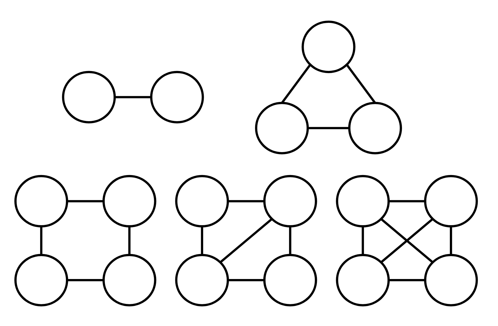
Figure 1: The statistical mechanical version of a ball and stick model.

The most exciting aspect for me (and likely for others in this field) is that there is still so much about liquids that remains unknown. Indeed, liquid state theory is not yet advanced enough to allow one to take a molecular description of a liquid and fully describe its structural, thermophysical, and flow properties. This challenge was recognized by theorists in the early 1960s, and owing to advancements in computing machines and numerical methods, led to the development of computer simulations of the liquid state. Computer simulations of liquids have since become one of the most widely used and successful methods for understanding chemical processes fundamental to energy storage and transfer, biological function and health, and even the behavior of interstellar bodies. Clearly, if a general liquid state theory were discovered, many of us molecular dynamicists might soon find ourselves out of a job!

Despite lacking a unified theory of the liquid state, what we know is that there are fundamental relationships between the arrangement and organization of molecules and emergent thermodynamic properties. The arrangement of molecules, which can be charted by a spherical coordinate system with vectors corresponding to the radial, polar, and azimuthal positions of atoms in the system, will be referred to as the structure of a liquid. Of course, our limited senses and technology make it practically impossible to know the structure at any instant, or snapshot, in time. However, measurement techniques such as X-ray and neutron scattering can be used to estimate the structure that the liquid takes on average. It is these averages of the atomic coordinates that can be used within existing liquid state theories to establish a connection to interatomic forces and thermodynamic behavior.

Correctly linking liquid structure with theoretical statistical mechanics holds great promise in engineering novel liquid state materials and advancing our fundamental understanding of the liquid state. Such a method could obviate the need for designing and training expensive computer simulations, inform engineers on subtle, atomic scale structure-property relationships, and possibly be used in tandem to ab initio electronic structure calculations to understand how quantum mechanical effects impact condensed phase properties. Finally, studying the connection between structure, atomic scale forces, and thermodynamics is of great theoretical interest. It pushes the boundaries of what can be learned from existing theories and has the potential to identify key problems with predominant schools of thought on the connection between atomic and thermodynamic behavior. Ultimately, such an approach could form a unified theory of liquids that comprehensively describes molecular, thermophysical, and continuum-scale behavior from a molecular perspective. Towards this ultimate goal, this dissertation aims to propose a novel interpretation of structure-potential modeling through the application of Bayesian probability theory.

To this aim, the remainder of this introduction will be organized as follows:

1. Measuring Liquid Structure with Experimental Neutron Scattering - Overview of liquid structure measurement techniques using neutron scattering experiments. It discusses fundamental mathematical relationships between observed quantities (e.g., the structure factor) and derived quantities (e.g., radial distribution functions), essential for interpreting liquid structure. Furthermore, it addresses key experimental and modeling challenges involved in extracting interatomic forces from structural data.

2. A Comprehensive Review of Structure-Potential Analysis - Literature review of state-of-the-art applications of liquid state theory in the analysis of neutron scattering data. It outlines key methods such as the Ornstein-Zernike integral relation, the Henderson inverse theorem, and empirical potential structure refinement. Additionally, a detailed yet concise proof of the Henderson inverse theorem is included, as it serves as the primary evidence for the hypothesis that a unique pair potential can be derived from scattering measurements for real liquids. This theorem also underpins the variational method of structure optimized potential refinement described in Chapter 2.

3. Modern Scattering Analysis: A New Perspective - Introduces the central thesis of the dissertation, emphasizing the potential of a novel perspective centered on uncertainty quantification. It defines and justifies the adoption of uncertainty quantification using Bayesian analysis and outlines its application within the text. Specifically, it discusses the implementation of Bayesian techniques for both continuous functions (Gaussian processes - Chapters 2-4) and discrete variables (Bayesian parameter optimization - Chapters 3 and 4).

1.2 Measuring Liquid Structure with Experimental Neutron Scattering

In statistical mechanics, the structure of a liquid is characterized using the radial distribution function, $g(r)$. This function is computed by counting the number of particles surrounding a reference particle and constructing a radial shell of thickness $dr$ around this particle. The average value of the radial distribution function at $r+dr$ is the particle number density within the shell divided by the bulk particle density of the material. This process is repeated for each particle in the system and over time, and the results are subsequently averaged. Thus, $g(r)$ represents a radial, time, and particle average density distribution. A visualization of a single snapshot of this computation is shown in Figure 2 (radial distribution function was taken from Yarnell (1974) [2]).

Neutron scattering is the gold-standard technique to measure radial distribution functions from sub-angstrom to micron length scales for systems with light-atoms (such as hydrogen) [3]. When a neutron beam is directed through soft matter, incident neutrons collide with atomic nuclei and scatter in various directions (Figure 3). A detector mounted behind the sample container is designed to quantify single neutron interaction events as a function of momentum transfer, yielding an experimental observable known as the differential scattering cross section, $\frac{d\sigma}{d\Omega}$. The scattering cross section is the ratio of scattered neutrons per second into solid angle $d\Omega$ divided by the number of neutrons incident to $d\Omega$ (which is just $d\Omega$ times the incident flux and has units of barns/steradian) and contains contributions from a wide array of neutron-atom interactions, including elastic, inelastic, incoherent, and multiple scattering [4].

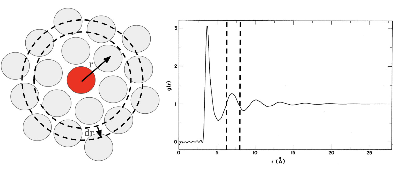
Figure 2: The radial distribution function keeps track of the particle density of a system as a function of radius away from a reference atom. The dashed radial shell in the particle picture (left) is represented as a radial interval in the radial distribution function (right).

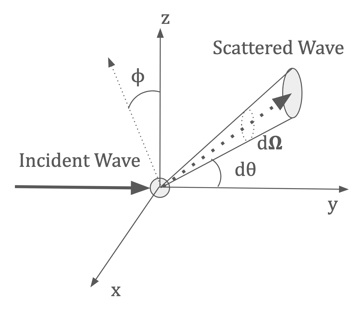
Figure 3: Incident scattering vector $\mathbf{k_{i}}$ scattered through solid angle $d\Omega$.

The time-averaged, elastic contribution to the scattering cross section, named the static structure factor, is the linear density response of the material to the neutron wave propagation momentum, $\hslash\mathbf{q}$. By the fluctuation-dissipation theorem, the linear density response of a perturbed system can be expressed in terms of equilibrium fluctuations in the unperturbed system. Therefore, the static structure factor measures the time-averaged, equilibrium particle density distribution in momentum space [5]. The static structure factor in a monatomic system with no long-range order is related to the more familiar radial distribution function, $g(r)$, through the radial Fourier transform,

$$S(q)=1+\frac{4\pi}{q\rho}\langle b\rangle^{2}\int_{0}^{\infty}r[g(r)-1]\sin(qr)dr$$ (1)

where $q$ is the momentum transfer, $b$ is the scattering length density, and $\rho$ is the atomic number density [6].

In mixtures or molecular liquids, the static structure factor, referred to in this case as the total structure factor $F(q)$, can be expressed as a combination of of site-site partial structure factors, $s_{ij}$, between atoms $i,j$ such that,

$$F(\mathbf{q})=\sum_{i\geq j}[2-\delta_{ij}]w_{ij}s_{ij}(\mathbf{q})$$ (2)

where $w_{ij}$ is a weighting factor depending on the scattering length density and atomic concentration of the $i,j$ pair and $\delta_{ij}$ is the Kronecker delta. Partial structure factors can be Fourier transformed with Eq. (1) to obtain real space site-site pair distribution functions. These site-site radial distribution functions show how the atomic density of type 1 within a spherical shell around any atom of type 2 in the system changes with respect to the radius of the shell. For example, in liquid water, an O-H partial distribution function describes atomic fluctuations of oxygen atoms around any arbitrary hydrogen atom. Eq. (2), referred to as the Faber-Ziman approximation, is ill-posed (since it has no unique solution) and can only be approximated via iterative molecular simulation approaches.

While eqs (1) and (2) hold true in theory, practical implementation of these models face several challenges. First, the finite size of individual neutron detectors constrains structure factor measurements to discrete momentum transfer, $\Delta q=q_{i}-q_{i-1}$, values which can result in aliasing if the sampling efficiency is $<1$ (i.e. the Peterson-Middleton theorem [7]). Second, finite detector coverage windows the measurement to a range between some $q_{\text{min}}$ and $q_{\text{max}}$, preventing the evaluation of the full integral specified in Eq. (1). Finally, measurement uncertainty of neutron counts and momentum transfer positions (i.e. time-of-flight uncertainty) introduce noise that can corrupt the underlying signal [8]. These limitations mean that we can only compute a discrete radial Fourier transform over uncertain observations,

$$g(r)\approx 1+\frac{1}{2\pi^{2}\rho}\sum_{q_{i}=q_{\text{min}}+q_{1}}^{q_{\text{max}}}\frac{\mathcal{S}(q_{i-1})-\mathcal{S}(q_{i})}{2}(q_{i}-q_{i-1})$$ (3)

where we have introduced the notation $\mathcal{S}(q)=S(q)\frac{\sin(qr)}{qr}q^{2}$ for brevity. The key problem here is that this discrete Fourier transform can introduce systematic deviations in the predicted $g(r)$ from the ground truth one.

The most well studied issue in prior literature is addressing the $q_{\text{max}}$ cutoff using so-called modification functions. The essential idea here is to smoothly transition the structure factor from a data dominated section (as measured by the neutron detector) to a model driven section (dictated by prior physical knowledge of the structure factor). Modification functions are designed to force the contribution of the experimental data to 0 near $q_{\text{max}}$, effectively nullifying any features in the data and strictly relying on the physical model alone. Usually the data is transitioned into is the Poisson point process ideal gas model (i.e. $S_{\text{Ideal}}(q)=1$)[9]. Mathematically, this adjusts the integral seen in equation 1 into,

$$g(r)=1+\frac{1}{2\pi^{2}\rho}\int_{0}^{\infty}(S(q)-1)M(q)\frac{\sin(qr)}{qr}q^{2}dq$$ (4)

where $M(q)$ is the modification function as a function of $q$. Common choices for the modification function are the first Bessel function [10], second Bessel function [11, 12], cosine cutoff [13], and dynamic functions [14]. However, as pointed out by J.E. Proctor and co-workers [15], this is an approximate Bayesian predictive model where the modification function is used to decide where a prior model of the $S(q)$ should be preferred over the data. This can be seen by rewriting equation 4 so that,

$$=1+\frac{1}{2\pi^{2}\rho}\int_{0}^{\infty}\bigg{(}\underbrace{(S(q)-1)M(q)}_{\text{Data Driven Predictive}}+\underbrace{(S_{\text{Ideal}}(q)-1)(1-M(q))}_{\text{Model Driven Predictive}}\bigg{)}\frac{\sin(qr)}{qr}q^{2}dq.$$ (5)

If you view $M(q)$ as discrete posterior probability mass, then this expression can be thought of as writing the structure factor as a weighted mixture of the two outcomes, either data or model, at each $q$ value.

1.3 A Comprehensive Review of Structure-Potential Analysis

At this point, it should be clear that the determination of radial distribution functions are obscured by experimental, model, and measurement uncertainty. However, assuming that the radial distribution functions can be determined accurately, there are a few fundamental liquid state theories that allow us to predict interatomic forces between atoms in the system and consequently their thermodynamic behavior. One of the most important and far reaching results is the Ornstein-Zernike (OZ) integral relation [16].

The OZ relation can be proven by noticing that the excess part of the free energy functional generates a set of direct correlation functions that can be related to the density correlation function [17]. Conceptually, all that we are doing is a statistical mechanical "book keeping" of the direct and indirect atomic correlations. Unfortunately, on its own the OZ relation is not enough to take an experimental scattering measurement and determine an interatomic potential. Instead, we introduce some approximation of how the direct correlation function is related to the interatomic potential using a closure relation. Practically, OZ integral relation methods generally have slow convergence; and further, owing to their approximate nature, often do not give accurate predictions for interatomic potentials and thermodynamic properties for real systems [18, 17]. It is notable, however, that the emergence of machine learning in liquid state theory has shown promise in mitigating these challenges [19]. For example, neural networks have been implemented to solve both the forward and inverse Ornstein-Zernike integral relations for simple liquids [20, 21]. Further note that there are other integral relations from liquid state theory, including the Yvon-Born-Green equation and the Bogoliubov–Born–Green–Kirkwood–Yvon (BBGKY) hierarchy, but these have seen little use for scattering analysis.

The Henderson inverse theorem, first published in 1974, is another important and more practical result on the relationship between the radial distribution function and pairwise additive potential in a statistical ensemble. The Henderson inverse theorem states that, given a fixed density, homogeneous system with pairwise additive Hamiltonian and the same radial distribution function, their pair potentials can differ by at most a trivial constant [22]. The importance of this result lies in the fact that, if one can find a potential that reproduces a target radial distribution function, this must be the unique (up to an additive constant) potential that models that system. Supposing that this pair potential was sufficient to model the interatomic forces, it is possible, in principle, to recover thermodynamic consistency with liquid state theories such as the Ornstein-Zernike relation.

To prove this theorem, we first need to establish the Gibbs and Gibbs-Bogoliubov inequalities for a quantum system. The Gibbs inequality is an important result about the information entropy of a system while the Gibbs-Bogoliubov inequality establishes a relationship between the free energy and entropy in the canonical ensemble.

Lemma 1.1.

Let $\rho_{1}$ and $\rho_{2}$ be positive, trace-class, and linear density operators on a Hilbert space, $H$, such that $Tr(\rho_{i})=1$. Then,

$$Tr(\rho_{1}\log(\rho_{2}))\leq Tr(\rho_{1}\log(\rho_{1}))$$

Proof.

We can express the states $\rho_{1}$ and $\rho_{2}$ in an arbitrary basis of $H$ (c.f Riesz’s Lemma [23]) such that,

$$\rho_{1}=\sum_{\alpha}p_{\alpha}\ket{\alpha}\bra{\alpha}$$

$$\rho_{2}=\sum_{\alpha}q_{\alpha}\ket{\alpha}\bra{\alpha}$$

We then compute the difference between the cross entropy, $\rho_{1}\log(\rho_{2})$, and information entropy of $\rho_{1}$, $\rho_{1}\log(\rho_{1})$,

$$\rho_{1}\log(\rho_{2})-\rho_{1}\log(\rho_{1})=\sum_{\alpha,\beta}[p_{\alpha}\ket{\alpha}\bra{\alpha}\log(q_{\beta})\ket{\beta}\bra{\beta}-p_{\alpha}\ket{\alpha}\bra{\alpha}\log(p_{\beta})\ket{\beta}\bra{\beta}]$$

and since ${\alpha}$ and ${\beta}$ are orthonormal bases,

$$=\sum_{\alpha}[p_{\alpha}\log(q_{\alpha})-p_{\alpha}\log(p_{\alpha})]\ket{\alpha}\bra{\alpha}.$$

Taking the trace of this operator we obtain,

$$Tr(\rho_{1}\log(\rho_{2})-\rho_{1}\log(\rho_{1}))=\sum_{\alpha}[p_{\alpha}\log(q_{\alpha})-p_{\alpha}\log(p_{\alpha})]=\sum_{\alpha}p_{\alpha}\log\frac{q_{\alpha}}{p_{\alpha}}.$$

Note that since $\log x\leq x-1$,

$$\sum_{\alpha}p_{\alpha}\log\frac{q_{\alpha}}{p_{\alpha}}\leq\sum_{\alpha}[q_{\alpha}-p_{\alpha}]=0$$

and finally, since the trace is a linear operator, this means that,

$$Tr(\rho_{1}\log(\rho_{2}))\leq Tr(\rho_{1}\log(\rho_{1}))$$

.

∎

Lemma 1.2.

Let $\rho_{1}$ and $\rho_{2}$ be positive, trace-class, and linear density operators on a Hilbert space, $H$, such that $Tr(\rho_{i})=1$. Then, in the canonical ensemble where, $\rho=\exp(-\beta\mathcal{H})/Z$, where $\beta$ is the inverse thermal energy, $\mathcal{H}$ is the Hamiltonian and $Z$ is the canonical partition function, then,

$$F_{2}\leq F_{1}+\langle\mathcal{H_{2}}-\mathcal{H_{1}}\rangle_{1}.$$

Proof.

Suppose we take the state $\rho_{2}$ in the canonical ensemble so that,

$$\rho_{2}=\exp(-\beta\mathcal{H_{2}})/Z$$

where $\beta$ is the inverse thermal energy, $\mathcal{H_{2}}$ is the Hamiltonian, and $Z$ is the partition function. Then for some $\rho_{1}$ we have,

$$Tr(\rho_{1}(-\beta\mathcal{H_{2}}-\log Z))\leq Tr(\rho_{1}\log(\rho_{1}))=-S_{1}/k_{B}$$

where $S_{1}=-k_{B}Tr(\rho_{1}\log(\rho_{1}))$ is the entropy of system 1 and $k_{B}$ is the Boltzmann constant. Since the trace is a linear operator, we can separate the argument of the trace on the left hand side and divide both sides by the thermodynamic $\beta$ to obtain,

$$Tr(\rho_{1}\mathcal{H_{2}})+k_{B}T\log Tr(Z)\geq+TS_{1}.$$

But $Tr(\rho_{1}\mathcal{H_{2}})$ is just the expectation of $\mathcal{H_{2}}$ over system state 1 and $-k_{B}T\log Tr(Z)$ is the definition of the Helmholtz free energy in the Canonical ensemble. Thus,

$$F_{2}\leq\langle\mathcal{H_{2}}\rangle_{1}-TS_{1}$$

and for system 1,

$$F_{1}\leq\langle\mathcal{H_{1}}\rangle_{1}-TS_{1}.$$

Combining the two expressions gives us the inequality,

$$F_{2}\leq F_{1}+\langle\mathcal{H_{2}}-\mathcal{H_{1}}\rangle_{1}.$$

∎

The content of Henderson’s inverse theorem can now be stated as follows:

Theorem 1.1.

Two systems with Hamiltonian’s of the form,

$$\mathcal{H}=\sum_{i}\frac{p_{i}^{2}}{2m}+\frac{1}{2}\sum_{i\neq j}u(|\mathbf{r_{i}}-\mathbf{r_{j}}|)$$

with the same radial distribution function, $g^{(2)}(\mathbf{r_{i}},\mathbf{r_{j}})$,

$$g^{(2)}(\mathbf{r_{i}},\mathbf{r_{j}})=\frac{1}{\rho^{2}}\bigg{\langle}\sum_{i}\sum_{j}\delta(\mathbf{r}-\mathbf{r_{i}})\delta(\mathbf{r}^{\prime}-\mathbf{r_{j}})\bigg{\rangle}$$

have pair potentials, $u(|\mathbf{r_{i}}-\mathbf{r_{j}}|)$, that differ by at most a trivial constant.

Proof.

Suppose that two systems with a pairwise additive Hamiltonian have equal radial distribution functions and $u_{1}-u_{2}\neq c$ where $c$ is some constant. Then,

$$\langle\mathcal{H_{2}}-\mathcal{H_{1}}\rangle_{1}\neq c$$

and since the Helmholtz free energies are constants,

$$F_{2}-F_{1}<\langle\mathcal{H_{2}}-\mathcal{H_{1}}\rangle_{1}$$

where we lose the possibility of equality from the Gibbs-Bogoliubov inequality. Now, we can expand the expectation of the Hamiltonian in terms of the radial distribution function (since the system is pairwise additive) so that,

$$F_{2}-F_{1}<\frac{n}{2}\int[u_{2}-u_{1}]g_{1}(\mathbf{r})d^{3}\mathbf{r}$$

and the same holds for a swap of the indices,

$$F_{1}-F_{2}<\frac{n}{2}\int[u_{1}-u_{2}]g_{2}(\mathbf{r})d^{3}\mathbf{r}.$$

Combining these two equations gives,

$$0<0$$

a contradiction. Therefore, our premise that the radial distribution functions are equal while the pairwise additive potential energies differ by a trivial constant must be false. The only other possible difference between the potential energies is constant, so this must be true to satisfy the Gibbs-Bogoliubov inequality.

∎

Analogous results can be proven more generally using the methods of relative entropy [24] and functional analysis (see Appendix D) [25, 26, 27], although it is notable that there is no guarantee that a unique potential exists for a given radial distribution function. And furthermore, these results take us no further in practice since the radial distribution function can only be inferred and not known exactly.

The Henderson inverse theorem forms the basis of modern numerical structure inversion methods including Schommers algorithm [28], iterative Boltzmann inversion (IBI) [29, 30], and empirical potential structure refinement (EPSR) [31]. Currently, IBI is generally used for training coarse-grained force fields from more computationally expensive all-atom force fields models, while EPSR is exclusively used to find molecular configurations that are consistent with experimental neutron scattering patterns [32, 33, 34].

IBI and EPSR are iterative predictor-corrector algorithms that can be summarized as follows: (1) a predictor is applied to ’predict’ the underlying interatomic potential given an experimental pair correlation function, (2) a corrector performs a molecular simulation (Monte Carlo molecular mechanics) with the predicted potential to evaluate the quality of fit between the simulated and experimental pair correlation functions, and (3) the corrector results are fed back to the predictor to refine or ’correct’ the prior potential. Steps 1-3 are iterated until the simulated and experimental pair correlation functions converge. While these methods can be used for coarse-graining or to determine molecular configurations consistent with a given scattering pattern, there is little evidence that interatomic potentials obtained from these techniques can reliably predict thermodynamic behavior for real liquids. For example, Soper showed that O-O and H-H site-site interatomic potentials derived from EPSR applied to scattering data of liquid water predict a 4 times more negative excess internal energy compared to the experimental value [31] and later concluded that EPSR cannot be used to derive a reliable set of site-site pair potentials for a given system [35].

In our search for a method that can fit experimental scattering data, estimate interatomic forces and model liquid state thermodynamics, clearly EPSR falls short. First, the molecular configurations and potentials generated from these methods can be wildly non-physical [36] and non-unique [37] (Figure 4). This lack of robustness maybe due to the specific construction of EPSRs Monte Carlo molecular mechanics step or because its solutions fluctuate on the whim of user-specified model inputs. Second, the fact that the determination of site-site partial structure factors is an ill-posed inverse problem performed on uncertain experimental data means that there is no unique molecular configuration that explains a given scattering measurement. The problem here is quite grave since, even if we did find a molecular configuration that matches the scattering data, there is no guarantee that this configuration makes any sense at all. Finally, it is well-known that there are significant quantum mechanical (both nuclear and electronic) and many-body effects that influence structural behavior in liquids that EPSR does not take into account in its molecular models. It is becoming increasingly evident that such effects significantly influence solvent behavior and self-assembly [38]. As methods to model these behaviors evolve and become more computationally accessible, the physical models underlying liquid structure prediction should evolve accordingly.

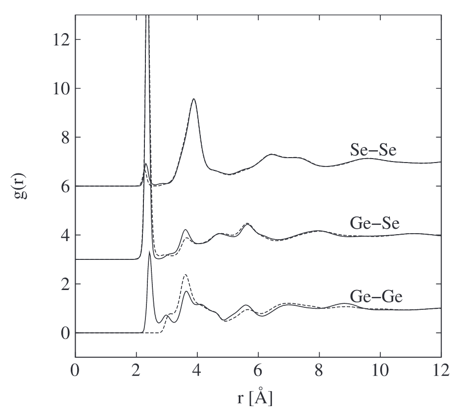
Figure 4: Site-site radial distributions for amorphous $GeSe_{2}$ determined from different EPSR runs differ by $\sim$16%. Figure reproduced from Alan Soper, On the uniqueness of structure extracted from diffraction experiments on liquids and glasses, Journal of Physics : Condensed Matter, Volume 19, Issue 41, Page 12, 01/01/1989. © IOP Publishing. Reproduced with permission. All rights reserved.

To summarize the current state-of-the-art, what we have is a scientific landscape where we can accurately measure atomic scale correlations between atoms in complex molecular liquids with neutron scattering experiments, along with multiple and sound theoretical results allowing us to connect this information to fundamental interatomic forces and thermodynamics. And yet, a clear demonstration of this connection has evaded the scientific literature for over a century. While interatomic potentials can be derived with existing tools like EPSR, the fact that the results are not robust, can change from run to run, and do not reproduce thermodynamic behavior suggests that existing techniques are generally unreliable and not suitable as a bridge between structure, interatomic forces, and thermodynamic properties. Therefore, what is needed is a careful reexamination of the philosophical, theoretical, and computational approaches to this complex inverse problem.

One could say that the problem of building thermodynamically consistent structure-potential models for liquids is similar to "finding a needle in a hay stack". But in fact, the situation is much worse since we wouldn’t be able to tell the difference between the needle and the hay even if we found it! A more accurate description could be summarized as "finding a specific needle in a needle stack".

1.4 Modern Scattering Analysis: A New Perspective

Based on the latest advancements in liquid structure modeling, the prevailing challenges that remain in the field can be outlined as follows:

1. Experimental scattering data is subject to numerous sources of random errors, arising from uncontrolled effects and improper data corrections and manipulations (e.g., Fourier transforms). Consequently, interpreting scattering measurements in real space is non-trivial and can introduce uncertainty into the observed structures used in liquid state theories.

2. The non-uniqueness of real-space structure interpretation implies that commonly used scattering analysis tools, such as EPSR, are sensitive to model parameter inputs and do not guarantee the same solution for each run. Additionally, the lack of uncertainty quantification in existing methods means we cannot gauge the reliability of the results.

3. Current state-of-the-art methods for the structure-potential inverse problem, such as the Ornstein-Zernike relation and Henderson inverse theorem based methods, are rigorously derived from statistical mechanics. These equations necessitate approximate closure relations, molecular simulations, or advanced machine learning algorithms (e.g., neural networks) to solve. Thus, these methods are often slow to converge and have primarily been successful only in simple fluid models, thereby limiting their practical utility in studying real liquids.

Clearly, uncertainty is the main thread that occludes every step towards a consistent structure-property model of liquids. First, the scattering data is uncertain, making it impossible to confirm if a ’correct’ measurement is being applied as the structure target. The statistical mechanical model and its parameters are also uncertain. For example, the Ornstein-Zernike equation may be rigorous for a system of classical particles, yet contains no description of important quantum mechanical effects of the electrons or nuclei. Moreover, the resulting solution lacks guaranteed uniqueness, leaving us unable to verify its accuracy without external validation through molecular simulations or thermodynamic calculations.

In this dissertation, it is my aim to outline an alternative philosophy to liquid state theory that centers on the key idea of making decisions in the face of uncertainty. Here uncertainty will refer to our current state of knowledge (i.e. the value of an observable within some credibility interval) given model, parametric, experimental, and computational uncertainties as defined below:

1. Model uncertainty refers to the fact that there is never a ’perfect’ model of nature that we can use to predict a quantity-of-interest. In the context of molecular simulations, model uncertainty is associated with choosing a specific force field, or choosing to use a path integral molecular dynamics method rather than an ab initio electron structure method.

2. Parametric uncertainty refers to the uncertainty in the parameters we use within a given model. For instance, the Lennard-Jones force field parameters for argon are $\sigma=3.4$ Åand $\epsilon=0.24$ kcal/mol. But how sure can we be that these are exactly correct parameters? What if I choose a slightly smaller or larger $\sigma$? Does it really effect the results of the molecular simulation? In reality, there is a distribution of parameters that can model a given quantity-of-interest, and we can think of this distribution as representing parametric uncertainty.

3. Experimental uncertainty refers to the fact that measurements are subject to numerous sources of error that make the data deviate from the ground truth. A straightforward example is noise in signals or systematic error from a thermocouple being poorly calibrated.

4. Computational uncertainty refers to uncertainty in numerical calculations. Although these errors can be quite small, floating point errors or misallocation of memory in parallel algorithms can cause deviations from true solutions, particularly in complicated numerical problems that require multiprocessing.

Bayesian methods are the gold-standard in treating these obscure types of uncertainty in a mathematically rigorous way. The idea is to learn the posterior probability distribution, $p(\theta|D)$ (read probability of $\theta$ given $D$), of some quantity-of-interest $\theta$ (this could be a parameter, model, function, field, etc), given observed data $D$ according to the following equation,

$$p(\theta|D)=\frac{p(D|\theta)p(\theta)}{p(D)}$$ (6)

where $p(D|\theta)$ is the likelihood that the data is well modeled by $\theta$, $p(\theta)$ is our prior, and $p(D)$ is the probability of $D$ being observed at all [39]. Note that no restriction has been imposed on the form of $\theta$, $D$, the likelihood or prior aside from the fact that any quantity $p(\cdot)$ must be a probability distribution (i.e. it must be non-negative and integrate to one over all possible events). In fact, $\theta$ can be a single quantity, tensor, function, or field and $D$ can be a list of many observations or a combination of completely different observations without loss of generality. If the quantity-of-interest is a function, then stochastic processes (e.g. Gaussian processes) are typically invoked using Bayesian nonparametrics [40] (see Appendix C).

Although Bayes’ Theorem is a straightforward statement of conditional probability, it is conceptually powerful. It provides a method for updating our beliefs about a hypothesis based on new evidence by combining prior knowledge with new data to revise the probability of the hypothesis being true. The flexibility in choosing likelihood and prior probability distributions has led some to criticize Bayesian statistics as being too subjective [41]. However, this flexibility allows for the incorporation of expert knowledge, ensuring that models remain realistic and physically plausible. This interpretability gives Bayesian inference a significant advantage over other black-box machine learning methods, such as neural networks or variational autoencoders, for function approximation and uncertainty quantification [42].

Bayesian inference finds diverse applications, ranging from training models to predicting outcomes with credibility estimates, and even forecasting functional and field distributions [43]. In essence, it offers a structured approach to compute both discrete probability mass densities and continuous probability distribution functions across parameters and quantities-of-interest. These probabilistic assessments are instrumental in decision theory applications, facilitating risk and loss quantification, as well as sensitivity analysis of model parameters in predicting outcomes. Moreover, they serve as invaluable guides in research, pinpointing gaps in existing models and directing further investigations. Remarkably, Bayesian field theory even reveals fundamental connections with statistical physics and quantum mechanics, offering insights into the complex phenomena of atomic systems [44].

At first, uncertainty can be a confusing concept, as it is not immediately clear how to express a ’lack of knowledge’ in a rigorous way. For this, we will need the tools of probability theory [45] and its numerical counterpart, probabilistic machine learning [43]. Probabilistic machine learning has experienced a renaissance in the last few decades, with applications becoming commonplace across a broad landscape of contemporary science including astronomy [46], ecology [47], and genetics [48, 49, 50, 51], among others. Liquid structure analysis is no different. In fact, it has been speculated that novel approaches to neutron scattering would likely be Bayesian in nature [37], and we are just starting to see probabilistic machine learning methods applied to neutron diffraction [52]. Uncertainties have been reported for the estimated partial radial distributions for water [53] (see Figure 5), although this is likely an underestimate since the analysis did not consider experiment, model or parameter uncertainty.

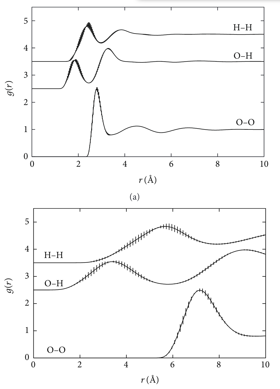
Figure 5: Partial radial distribution functions for HH, OH, OO atom pairs with uncertainty estimates from 6 EPSR runs (vertical bars). Figure reproduced from Alan Soper, The Radial Distribution Functions of Water as Derived from Radiation Total Scattering Experiments: Is There Anything We Can Say for Sure?, ISRN Physical Chemistry, Volume 2013, 11/28/2013.

This dissertation hypothesizes that rigorous uncertainty quantification using Bayesian inference can enhance the capabilities of liquid state theory and address its primary challenges. For instance, applying Bayesian uncertainty quantification to experimental scattering data can reduce the risk of overfitting to poor data. Additionally, recognizing that model results come from a distribution of possible solutions allows for the quantification of non-uniqueness and lack of robustness in a given model. Using Bayesian Gaussian processes to quantify this distribution enables us to learn model outputs with uncertainty, even for complex functions like the pair potential (Chapter 2) and structural correlation functions (Chapters 3 and 4). Furthermore, physics-informed Gaussian process design can ensure that the model predictions abide by physically justified principles such as continuity and differentiability, mitigating non-physical solutions often observed from EPSR. Bayesian optimization can also estimate model and parameter uncertainty within a selected model framework (Chapters 3 and 4), helping to determine whether a model choice is adequate for explaining a given quantity of interest.

1.5 Outline and Scope of the Thesis

The main content of this dissertation includes three chapters in which a novel application of Bayesian inference is applied to advancing the start-of-the-art in structure-property models. Chapter 2 is a reproduction of my first paper, "Transferable force fields from experimental scattering data with machine learning assisted structure refinement" originally published in the Journal of Physical Chemistry Letters in December, 2022. The chapter describes how to implement nonparametric Bayesian methods, specifically Gaussian process regression, within an iterative Boltzmann inversion framework to learn interatomic potentials from neutron scattering data in noble liquids. Chapter 3 shifts gears and focuses on a practical method to train molecular models given experimental scattering data using Bayesian inference. The idea is to use machine learned "surrogate" models to replace the molecular dynamics step in the model parameter training, effectively reducing the force field training time by over a million-fold. Chapter 3 is a reproduction of the paper, "Accelerated Bayesian inference for molecular simulations using local Gaussian process surrogate models", published in the Journal of Chemical Theory and Computation in March, 2024. Chapter 4 explores the questions (1) how accurate does scattering data need to be to learn underlying interatomic forces and (2) do random errors from scattering measurements corrupt the structure measurement to a degree that we can no longer recover interatomic force information? A question originally investigated by Verlet in 1968, this chapter demonstrates that the prior conclusion that it was not possible to quantify interatomic forces from scattering data may need to be overturned. Chapter 5: Conclusions and Future Work outlines key results and motifs from the thesis and expands on ongoing and future research on the horizon of Bayesian liquid state theory.

Finally, four appendices are included for reference to specific topics and/or mathematical concepts addressed in the main chapters: (A) Quantum and Many-Body Effects from Neutron Scattering expands on ongoing work attempting to decipher what physical phenomenon induce specific features in SOPR potentials. (B) Statistical Mechanics of Liquid Phase Systems is a collection of personal notes starting with classical Hamiltonian mechanics through to statistical mechanics of the liquid state. These notes were compiled and prepared as a lecture series for the course, "Molecular Simulations for Chemical Engineers" taught in Fall, 2023 at the University of Utah and have an accompanying video lecture series on YouTube
(https://www.youtube.com/playlist?list=PLmVLYa8E5SDff-uE7ehWBsX5sQzVRYiG6).
The course was taught by the support of the Utah Teaching Assistantship program. (C) Principles of Bayesian Statistics outlines the basics of probability theory and Bayesian methods as implemented in the main chapters. Although this appendix is not suitable to replace a full text on the subject (I would recommend Gelman’s Bayesian Analysis [39]), the hope was to briefly outline key terminology and results that were not expanded on in the main chapters. Finally, Appendix (D) Introduction to Functional Analysis is included as a reference to terminology and theorems relevant to understanding some of the most recent results in liquid state theory. Particularly relevant are a series of papers outlining the applicability, limitations, and practical variational implementations of the Henderson inverse theorem [25, 26, 27] as well as providing a basis to understand Bayesian field theory [44]. Although not directly used in the main chapters, I felt that it was important to compile and include these notes for future reference as the methods of functional analysis may offer exciting new ways of conceptualizing important problems in the field.

2 Learning Interaction Potentials from Scattering Data

Structure and interatomic forces are fundamentally linked. Although these relationships can be rigorously established for model fluids, the situation is less optimistic for real systems due to significant many-body interactions and quantum mechanical effects. However, fundamental results from statistical mechanics, such as the Ornstein-Zernike integral relations, inverse Kirkwood-Buff theory, and the Henderson inverse theorem (see Appendix B), hint at the possibility of determining unique and accurate interaction potentials to model thermodynamic and structural property relationships simultaneously. These force fields would be better suited to studying complex behaviors of liquids, such as self-assembly or vapor-liquid equilibrium, and possibly give insight into the nature of physical interactions.

We have developed an algorithm called structure-optimized potential refinement (SOPR) designed to extract interaction potentials from experimental scattering data. SOPR is a numerical method for the Henderson inverse theorem assisted by probabilistic machine learning to address challenges such as over-fitting to uncertain data and numerical instability. The probabilistic machine learning step involves Gaussian process regression with physics-guided priors of the interaction potential estimated with Henderson inverse theorem. SOPR has been applied to radial distribution functions on noble gases and found to be transferable to the prediction of vapor-liquid equilibria, demonstrating for the first that potentials derived directly from a scattering measurements can reproduce thermodynamic properties of real fluids. In this chapter, the original publication describing the foundational principles and SOPR method is reproduced from the Journal of Physical Chemistry Letters, 13 (49), 11512-11520 with permission of the publisher.

2.1 Abstract

Deriving transferable pair potentials from experimental neutron and X-ray scattering measurements has been a longstanding challenge in condensed matter physics. State-of-the-art scattering analysis techniques estimate real-space microstructure from reciprocal-space total scattering data by refining pair potentials to obtain agreement between simulated and experimental results. Prior attempts to apply these potentials with molecular simulations have revealed inaccurate predictions of thermodynamic fluid properties. In this letter, a machine learning assisted structure-inversion method applied to neutron scattering patterns of the noble gases (Ne, Ar, Kr, and Xe) is shown to recover transferable pair potentials that accurately reproduce both microstructure and vapor-liquid equilibria from the triple to critical point. Therefore, it is concluded that a single neutron scattering measurement is sufficient to predict macroscopic thermodynamic properties over a wide range of states and provide novel insight into local atomic forces in dense monoatomic systems.

2.2 Introduction

Advances in neutron and X-ray scattering analysis have significantly furthered our understanding of self-assembly and dynamic transport properties in dense fluid systems [54, 55]. Scattering analysis is therefore an important and necessary component in the development and validation of atomistic force fields aimed at predicting both micro- and macroscopic thermodynamic properties over a wide range of states. However, strikingly contradictory predictions between experimental and simulated microstructures have been reported in relatively simple systems, including monoatomic liquid metals [56], aromatic hydrocarbons [34], and water [57]. Given the proliferation of accessible neutron and X-ray scattering instrumentation, advances in computational analysis, and development of machine learning approaches, it is relevant to revisit whether scattering data can improve force fields for fluid property predictions and provide insight into local atomic forces.

One approach to benchmark force fields to scattering data is to calculate the underlying interatomic potentials from the experimental pair correlation functions, the so-called inverse problem of statistical mechanics. A number of well-established inversion techniques have been proposed, including Ornstein-Zernike (OZ) integral relation methods [16, 58, 59, 60, 61], Yvon-Born-Green (YBG) theories [62, 63, 64, 65, 66], Schommer’s algorithm [28], hypernetted chain methods [18, 67], the generalized Lyubartsev–Laaksonen approach [68, 69, 70], empirical potential structure refinement (EPSR) [31], and a neural network [71]. However, there is little evidence that interatomic potentials obtained from these techniques can reliably predict thermodynamic behavior for real liquids. For example, Soper showed that O-O and H-H site-site interatomic potentials derived from EPSR applied to scattering data of liquid water predict a 4 times more negative excess internal energy compared to the experimental value [31] and later concluded that EPSR cannot be used to derive a reliable set of site-site pair potentials for a given system [35]. A recent scattering study on supercritical krypton found rapid short-range oscillations in EPSR-derived interatomic potentials that led the authors to conclude that augmentation of the EPSR algorithm is required to obtain a more accurate representation of the real physical system [36]. Additionally, the remaining studies on structure-inversion of real liquids reported no validation of the interatomic potentials to predict fluid properties [72, 73, 74, 75, 76]. Notably, in a review of structure-inversion methods it is opined that the general purpose of these techniques is not to derive or evaluate interatomic potentials, but rather to determine molecular configurations that are consistent with the scattering data [77]. Therefore, it remains to be shown if scattering derived potentials can predict atomic trajectories consistent with experimental scattering measurements while also accurately modeling other thermodynamic properties.

The atomic length scale probed by experimental scattering measurements also confers an additional opportunity, specifically whether it is possible to learn details of the local interactions independent of assumptions on a specific model potential form (e.g., 12-6 Lennard-Jones). For example, the rate of short-range repulsive decay indicates the propensity of an atom to deform in a collision, such that relaxation from an infinitely steep potential wall to a finite exponential or power-law decay represents the transition from hard- to soft-particle collision dynamics. The approximate collision diameter may be estimated by the radial position where the potential energy intersects zero, and the pairwise radial separation of zero force describes the effective dispersion energy. Provided structure-optimized potentials demonstrate the ability to predict emergent thermodynamic properties, their application provides a bridge between local atomic physics and continuum behavior.

2.3 Results and Discussion

In this letter, force fields were determined for four noble liquids (Ne, Ar, Kr, Xe) using a machine-learning augmented Schommer’s algorithm, referred to as structure-optimized potential refinement (SOPR), to refine pair potentials and obtain convergence between simulated and experimental pair distribution functions. Modifications to an initial reference potential are informed by numerical implementation of the point-wise Henderson’s inverse theorem and augmented via Gaussian process regression with a squared-exponential kernel function described in Equations (17) and (20), respectively. The structure-optimized potentials predict excellent representations of both the experimental pair distribution functions (Figure 6) and saturated vapor-liquid fluid properties. Consequently, structure-optimized potentials are validated using experimentally-consistent observations on both the micro- and macroscopic length scales, motivating the analysis of specific properties of the generated potentials. Additionally, the monoatomic structure and spherical symmetry of the noble gas system facilitates the comparison of the structure-optimized potentials (Figure 7) to reference ab initio potentials obtained in the low-density state from coupled cluster theory [78, 79, 80, 81], referred to as reference quantum dimer potentials. This comparison reveals state-dependent changes of many-body forces present in the experimental systems that were collected at states with varying reduced temperatures ($T_{r}$) relative to the critical point.

Figure 6: Reference potential radial distribution functions (grey dotted line) compared to the converged simulated radial distribution functions (blue circles) and experimental radial distribution functions (black line). Inset figures show the first solvation shell of the radial distribution function.

The structure-optimized potentials collected for fluids near their critical point (Ne-42K, Kr-199K, Xe-274K at $T_{r}=0.95$) exhibit softer repulsive decay, insignificant change to the collision diameter, and a substantial reduction in dispersion energy with respect to reference quantum dimer potentials. Thus, the ensemble averaged many-body behavior near the critical point results in softer particle collisions with decreased particle attraction. Near the triple point (Ar-85K at $T_{r}=0.56$), structure-optimized potentials show no significant change in the repulsive exponent, a 1.5 $\%$ increase in collision diameter, and a reduction in dispersion energy (Figure 7(b)) compared to the quantum dimer potential. Many-body effects therefore had a negligible effect on the particle stiffness while decreasing particle attraction near the triple point. The observation that the dispersion energy correction was relatively smaller for the near triple point potential compared to the near critical point potentials suggests that the dispersion energy is a function of the thermodynamic state, which is discussed in the context of temperature-dependent many-body effects later.

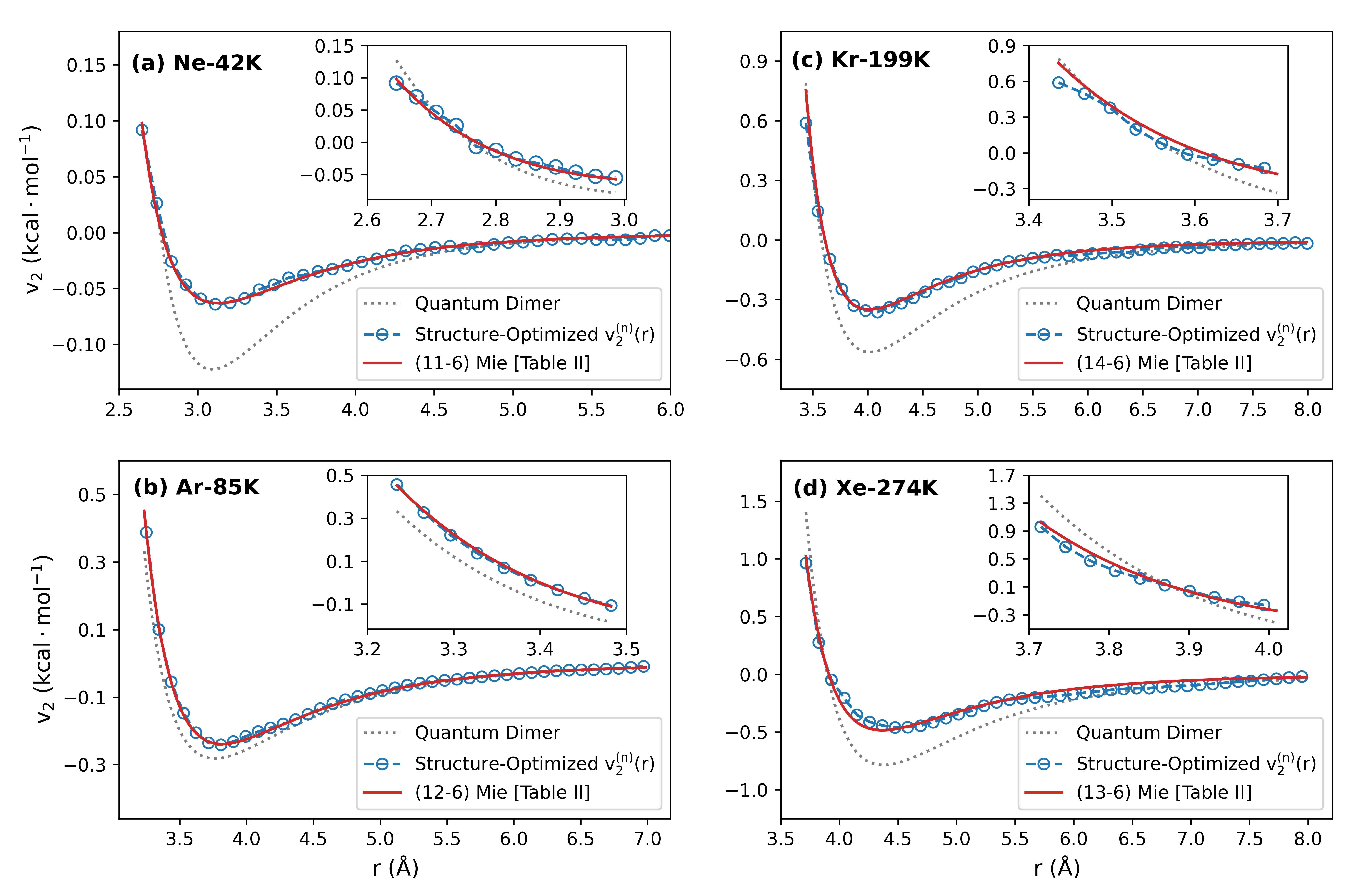
Figure 7: Tabulated structure-optimized potentials (blue) and $(\lambda-6)$ Mie potentials determined with Bayesian regression (red) are shown with reference quantum dimer potentials (grey). Inset figures show the short-range repulsive region of the corresponding structure-optimized potential.

It is instructive to compare the structure-optimized potentials to widely employed transferable pair potential functions, such as the ($\lambda-6)$ Mie potential,

$$v^{Mie}_{2}(r)=\frac{\lambda}{\lambda-6}\bigg{(}\frac{\lambda}{6}\bigg{)}^{\frac{6}{\lambda-6}}\epsilon\bigg{[}\bigg{(}\frac{\sigma}{r}\bigg{)}^{\lambda}-\bigg{(}\frac{\sigma}{r}\bigg{)}^{6}\bigg{]}$$ (7)

where $\lambda$ is the short-range repulsion exponent, $\sigma$ is the collision diameter (Å), and $\epsilon$ is the dispersion energy (kcal $\cdot$ mol^-1) [82]. The ($\lambda-6)$ Mie potential offers increased flexibility over the standard $(12-6)$ Lennard-Jones potential since the repulsion exponent may be varied to produce a wider array of potential shapes. Structure-optimized potentials were fit to the ($\lambda-6)$ Mie function via Bayesian regression and plotted as red lines in Figure 7. Note that the excellent quality-of-fit of structure-optimized potentials to the ($\lambda-6)$ Mie function indicates that the fitted parameters (listed in Table 1) can closely approximate the thermodynamic predictions of the tabulated structure-optimized potentials.

Table 1: Summary of ($\lambda-6)$ Mie potential parameters determined by Bayesian linear regression and modifications to the reference quantum dimer potentials in terms of the ($\sigma,\epsilon)$ parameterization. $\Delta\sigma$ and $\Delta\epsilon$ are shown as percent deviations from the ab initio parameter values given in Table 3.

Element	$\lambda$	$\sigma$ (Å)	$\epsilon$ (kcal/mol)	$\Delta\sigma$ (%)	$\Delta\epsilon$ (%)
Ne	11	2.77	0.063	0.31	-48.4
Ar	12	3.40	0.239	1.50	-16.7
Kr	14	3.58	0.359	-0.08	-38.3
Xe	13	3.91	0.484	0.51	-40.3

Transferability of the potentials was assessed by performing vapor-liquid equilibrium (VLE) calculations from the triple to critical point using histogram-reweighting grand canonical Monte Carlo (GCMC) simulations in the GPU-Optimized Monte Carlo (GOMC) simulation package [83] (see Supporting Information). Figure 8 shows vapor and liquid densities for structure-optimized potentials fit to $(\lambda-6)$ Mie potentials (red triangles) compared with experimental data (black lines) compiled from the National Institute of Standards and Technology (NIST) [84]. The Ne-42K structure-optimized force field predicts liquid densities within 0.1-2.5$\%$ relative error between 30-40K, on par with the top-performing Lennard-Jones force field from Vrabec et al. [85] and outperforming the next closest model [86] by as much as 10$\%$. The Ar-85K, Kr-199K, and Xe-274K force fields are less accurate, with liquid density relative errors of 0.2-5$\%$ (85-140K), 6.2-10.1$\%$ (120-180K) and 4.7-8.4$\%$ (190-260K), respectively. Simulated critical points determined with the Ising-type critical point scaling law [87] and law of rectilinear diameters [88] are provided in Table 2.

Table 2: Simulated critical temperatures ($T^{sim}_{C}$) and densities ($\rho^{sim}_{C}$) with statistical uncertainty calculated from 5 independent GCMC simulations. Percent error between simulated and experimental critical temperature and density are also shown.

Element	$T^{sim}_{C}$ (K)	$T^{err}_{C}$ (%)	$\rho^{sim}_{C}$ (kg/m3)	$\rho^{err}_{C}$ (%)
Ne	43.84 $\pm$ 0.06	-1.33	488.4 $\pm$ 1.08	0.91
Ar	154.27 $\pm$ 0.16	2.40	528.9 $\pm$ 0.84	-1.32
Kr	216.58 $\pm$ 0.60	3.36	952.7 $\pm$ 3.62	5.04
Xe	300.99 $\pm$ 0.28	3.98	1142.9 $\pm$ 1.76	4.85

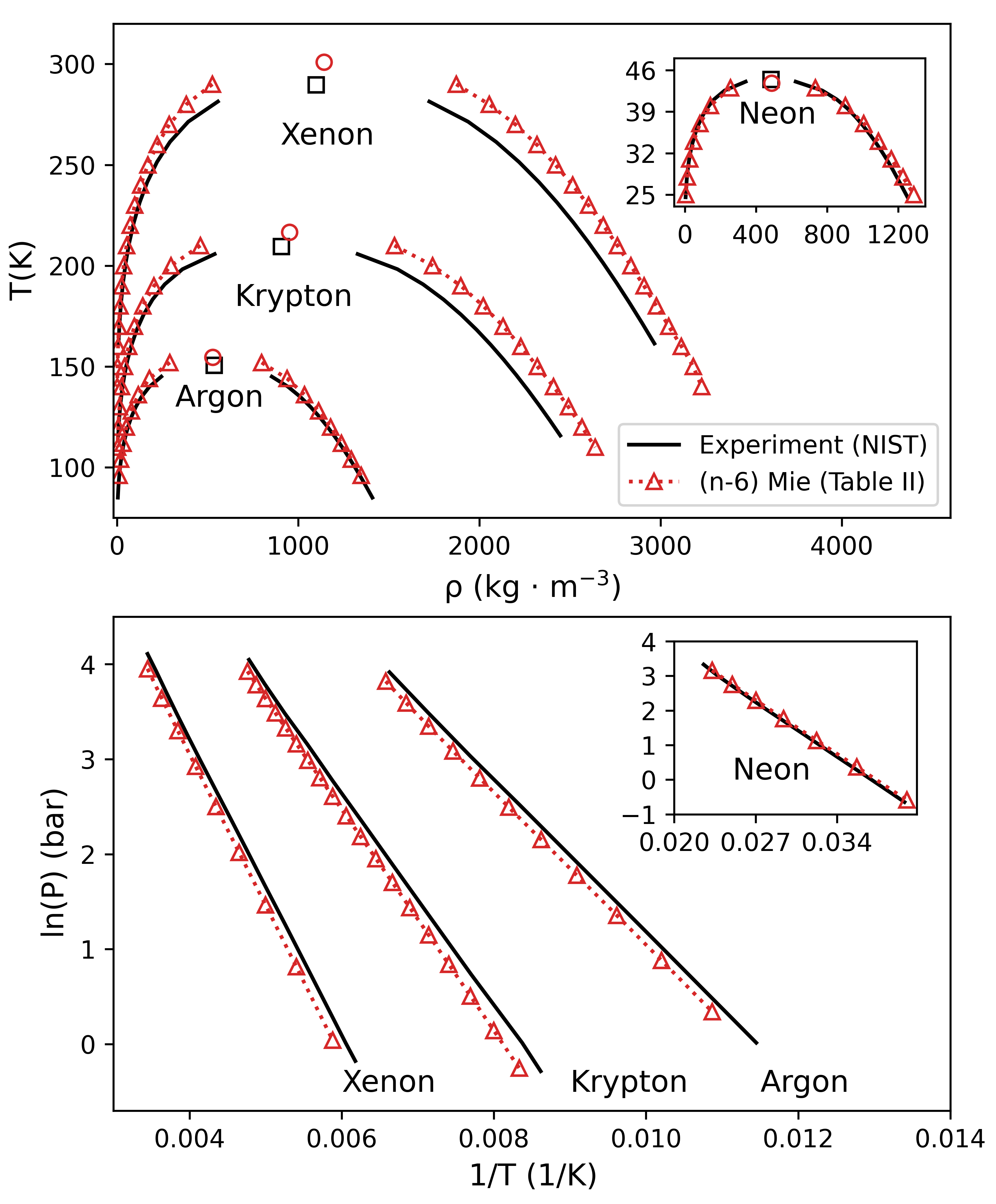
Figure 8: (Top) Simulated phase coexistence curves (red triangles) are shown with experimental phase data (black lines). Simulated and experimental critical points are given by the open red circle and open black square, respectively. (Bottom) Clausius-Clapeyron plots of the simulated pressure (red triangles) compared to experimental pressures (black lines).

A recently developed series of $(\lambda-6)$ Mie force fields benchmarked to noble gas vapor-liquid equilibrium (VLE) provides an excellent comparison to the structure-optimized force fields proposed in this work. In general, both force fields predict similar repulsion exponents ($\lambda$) and dispersion energies ($\epsilon$). One interesting observation is that both the structure and VLE-optimized force fields predict an increase in the repulsive exponent with increasing atomic weight. Mick et al. [89] demonstrated that varying the repulsive exponent improved the simultaneous prediction of saturated densities and vapor pressures, supporting the conclusion that static structure is sensitive to subtle variations in the pair potential. The most consequential difference between the two models is that the structure-optimized force field gives systematically lower predictions for the collision diameter ($\sigma$), causing the simulated liquid density to be overestimated compared to the experimental value. It is notable that the reported differences in the collision diameter (0.01-0.05 Å) are approximately one order of magnitude smaller than the real-space resolution of the experimental diffraction data (0.4-0.7 Å). Modern, high-flux scattering instruments can achieve real-space resolution of approximately 0.05 Å, on the same order as the error in the collision diameter, suggesting that more accurate potentials may be determined from repeating neutron scattering measurements on noble gases with modern instruments [8].

The observation that structure-optimized potentials can estimate vapor-liquid coexistence behavior from a single neutron scattering measurement suggests that structure-inversion may be a promising approach to develop force fields for materials where experimental phase behavior is absent or impractical to obtain. The phase behavior and criticality of liquid uranium (U) is one of many important and unresolved examples relating to nuclear reactor design and safety analysis. Neutron diffraction data on solid $\beta$-U exists to temperatures as high as 1045K [90] and X-ray diffraction patterns of $\gamma$-U close to the melting point (1405K) are well-characterized [91], but the phase coexistence line and critical point remain unknown, with critical temperature predictions ranging from 5000-13000K [92]. However, our results suggest that scattering measurements of liquid U may enable estimation of vapor-liquid phase coexistence via GCMC simulations with a structure-optimized embedded atom model or set of state dependent structure-optimized potentials.

Structure-inversion may also enable quantification of liquid state many-body effects. Quantum calculations on Kr-Ar-Ar and Ar-Ar-Kr trimers have revealed that noble gases experience two important many-body effects: (1) 3-body exchange repulsion and (2) the exchange/dispersion quadropole induced dipole [93]. The averaged pairwise influence of these many-body interactions decreases the short-range repulsion exponent and the dispersion energy [94], which is in agreement with the behavior observed in the structure-optimized potentials obtained near the critical point. Self-consistent field calculations of electron distributions in Ar clusters have shown that the electron cloud is compressed at higher densities, and that this compression reduces the probability of exchange repulsion [95]. Additionally, experimental results from collision-induced depolarized light scattering on compressed H₂ demonstrated that exchange-dependent many-body interactions become more prominent with increasing temperature [96]. It is therefore expected that many-body effects in noble gases should be less dominant near the triple point, explaining why the short-range decay rate for the Ar-85K structure-optimized potential was unchanged and the well-depth correction smaller than in the near critical point states. This conclusion is also supported by analyzing trends in the structural many-body correction for each fluid at near triple and critical point conditions (see Supporting Information). Further analysis with quantum mechanical and explicit 3-body dispersion models, such as the Axilrod-Teller potential [97, 98, 99], are reserved for future study on high-resolution scattering data sets obtained with state-of-the-art neutron techniques.

We demonstrate that transferable pair potentials can be reconstructed from a single neutron scattering measurement for monoatomic liquids, and further; that structure-inversion techniques have fundamental and interdisciplinary applications bridging experimental scattering, molecular simulation, and quantum mechanics. Of particular interest is the prediction of thermodynamic properties at extreme conditions, such as high temperature and pressure materials, molten salts, and liquid metals. The inclusion of experimental diffraction results for optimizing effective pair potentials may also facilitate improvements to local structure predictions for fluid mixtures and molecular liquids. However, incoherent and inelastic scattering corrections [4], as well as non-uniqueness of the partial structure factor decomposition, will need to be addressed to extend the presented techniques to complex liquids. Finally, the methods presented in this letter may be applied to benchmark force fields for coarse-grained simulations, which has seen a growing interest in structure-inversion techniques [100, 101].

2.4 Theory and Computational Methods

The following section provides the relevant definitions, statistical mechanics, and necessary computational details of the proposed machine learning assisted structure refinement method. First, the microstructure is considered as the local atomic density correlation and is formalized by counting the number of atomic neighbors as a function of position with respect to a reference atom and taking the ensemble average,

$$g(\mathbf{r})=\frac{1}{\rho}\bigg{\langle}\frac{1}{N}\sum_{i=1}^{N}\sum_{j=1}^{N}\delta^{3}(\mathbf{r}-\mathbf{r}_{j}+\mathbf{r}_{i})\bigg{\rangle}$$ (8)

where $g(\mathbf{r})$ is referred to as the radial distribution function, $\delta^{3}$ is the three-dimensional Dirac delta function, $\rho$ is the thermodynamic density and $N$ is the total number of particles in the system. The radial distribution function and pair correlation function, $h(\mathbf{r})$, are related by, $h(\mathbf{r})=g(\mathbf{r})-1$. Due to the lack of long-range order in liquids, the isotropically-averaged radial distribution function is related to the experimentally observed structure factor, $S(Q)$, which for a monoatomic liquid is given by,

$$S(Q)=1+\frac{4\pi}{Q\rho}\frac{\langle b\rangle^{2}}{\langle|f(Q)|^{2}\rangle}\int_{0}^{\infty}r[g(r)-1]\sin(Qr)dr$$ (9)

where $Q$ is the momentum transfer, $b$ is the scattering length density, $f(Q)$ is the form factor, and $\rho$ is the atomic number density [6].

The potential energy can be written as a sum of $n$-body potential energy terms such that,

$$U(\mathbf{r})=\overbrace{\sum_{i}^{N}v_{1}(\mathbf{r}_{i})}^{\text{external field}}+\overbrace{\sum_{i=1}^{N}\sum_{j\neq i}^{N}v_{2}(\mathbf{r}_{ij})}^{\text{two-body}}+\overbrace{\sum_{i}^{N}\sum_{j\neq i}^{N}\sum_{k\neq j}^{N}v_{3}(\mathbf{r}_{ijk})+...}^{\text{many-body}}$$ (10)

where $v_{p}(\mathbf{r}_{1,...,p})$ is a position dependent function that assigns a potential energy to a subset containing $p\leq N$ atoms for a given configuration $\mathbf{r}_{i,...,p}$ [102]. We further simplify this expression by neglecting the external field contribution ($p=1$) and averaging higher-order many-body terms ($p\geq 3$) into a state-dependent pair term,

$$\begin{split}U(\mathbf{r};\rho,T)&=\sum_{i=1}^{N}\sum_{j\neq i}^{N}\bigg{[}v_{2}(\mathbf{r}_{ij})+v_{2}^{m}(\mathbf{r}_{ij};\rho,T)\bigg{]}\end{split}$$ (11)

such that $v_{2}^{m}(\mathbf{r}_{ij};\rho,T)$ is explicitly dependent on the atomic positions and implicitly dependent on the physical state (temperature, density, etc). The bracketed quantity in Equation (11) is defined as the effective pair potential,

$$v_{2}^{eff}(\mathbf{r}_{ij};\rho,T)=v_{2}(\mathbf{r}_{ij})+v_{2}^{m}(\mathbf{r}_{ij};\rho,T)$$ (12)

which cannot be determined exactly for a state-dependent ensemble [103] but can be optimized to reproduce a set of experimentally observed thermodynamic properties, such as structure [104], heat of vaporization [105], or vapor-liquid equilibrium [83]. The pair potential defined in Equation (12) is the most common non-bonded term in the Hamiltonian of classical force fields and is typically modeled as a hard-particle, Lennard-Jones, $(\lambda-6)$ Mie, Buckingham, or Yukawa potential.

Pairwise additivity imposes important theoretical constraints on the relationship between the potential energy and pair correlation function. Henderson proved that for pairwise additive, constant density ensembles that there exists a one-to-one map between the effective pair potential and the radial distribution function up to an additive constant [22, 106, 26]. In monoatomic liquids with spherical symmetry, the structure-potential uniqueness theorem on a finite radial interval $[r^{\prime},r^{\prime\prime}]$ such that $r^{\prime\prime}>r^{\prime}$ and $r^{\prime},r^{\prime\prime}\in\mathbb{R}_{0}^{+}$, is equivalent to,

$$\int_{r^{\prime}}^{r^{\prime\prime}}\Delta v_{2}(r)\Delta g(r)\,dr\leq 0$$ (13)

where $\Delta v(r)$ and $\Delta g(r)$ are the difference between a model (M) and target (T) pair potential and radial distribution function, respectively [107].

$$\Delta v_{2}(r) =v_{2}^{M}(r)-v_{2}^{T}(r)$$ (14)

$$\Delta g(r) =g^{M}(r)-g^{T}(r)$$

Note that the structure-potential uniqueness theorem in the form of Equation (13) is written in terms of the $r$-coordinate only due to spherical symmetry. Initially, Equation (13) appears uninformative since the inequality prevents direct calculation of the target potential at any $r$ value. The situation is amenable under the assumption that the integrand is continuous and differentiable, so that Equation (13) can be rewritten using the mean value theorem,

$$(r^{\prime\prime}-r^{\prime})\bigg{\langle}\Delta v_{2}(r)\Delta g(r)\bigg{\rangle}_{r^{\prime}}^{r^{\prime\prime}}\leq 0$$ (15)

where the bracketed quantity represents the average of $\Delta v_{2}(r)\Delta g(r)$ over finite interval $[r^{\prime},r^{\prime\prime}]$. Notice that for this inequality to be satisfied in the limit $(r^{\prime\prime}-r^{\prime})\to 0$, it must hold at any point $r_{o}\in r$ so that,

$$\Delta v_{2}(r_{o})\Delta g(r_{o})\leq 0$$ (16)

which is true only when $\Delta v_{2}(r_{o})\neq 0$ and $\Delta g(r_{o})\neq 0$. The practicality of this point-wise structure-potential uniqueness theorem is now clear, since Equation (16) prescribes what direction that an initial guess for the model potential should be corrected given the difference between the model and target experimental radial distribution function at any point $r_{o}\in r$; namely, by decreasing the potential if $\Delta g(r_{o})$ is negative and increasing the potential if $\Delta g(r_{o})$ is positive. While Henderson’s structure-potential uniqueness condition has been implemented previously to obtain empirical estimates of pair potential functions in Schommer’s algorithm and EPSR, this derivation demonstrates the validity of its use at an arbitrary point without the potential of mean force approximation $g(r)=\exp[-\beta v_{2}^{eff}(r_{ij};\rho,T)]$ where $\beta=\frac{1}{k_{B}T}$, which only holds in the dilute limit [17].

The structure-potential uniqueness condition is implemented via iterative refinement of a reference potential, $v_{2}^{0}(r_{i})$, with an energy scaled, continuous sum of the radial distribution function error such that,

$$v_{2}^{(n)^{\prime}}(r_{i})=v_{2}^{0}(r_{i})+\gamma\beta^{-1}\sum_{n}\Delta g^{(n)^{\prime}}(r_{i})$$ (17)

where $i$ is the radial index of the tabulated potential, $v_{2}^{(n)^{\prime}}(r_{i})$ is the predictor estimated pair potential at iteration $n$, $\beta$ is the inverse thermal energy $(k_{B}T)^{-1}$, and $0<\gamma\leq 1$ is an empirical scaling constant to dampen the potential correction. Comparing the refinement Equation (17) to Equation (12), it is clear that if $v_{2}^{0}(r_{i})$ is selected as the quantum dimer potential that $v_{2}^{(n)^{\prime}}(r_{i})$ is the estimated effective pair potential and $\gamma\beta^{-1}\sum_{n}\Delta g^{(n)^{\prime}}(r_{i})$ is the pair averaged many-body term. Note that the prime notation in $v_{2}^{(n)^{\prime}}(r_{i})$ denotes that the pair potential is the predictor estimate before smoothing and treatment of numerical and experimental uncertainty.

In a standard Schommer’s algorithm, the potential predicted by Equation (17) is passed to the next iteration without smoothing or uncertainty quantification, which has been shown to reduce the methods robustness [18, 77]. Here a squared-exponential kernel Gaussian process (GP) is applied to the predictor estimate to account for numerical fluctuations arising from the molecular dynamics simulations as well as systematic over-fitting to uncertain experimental data. A GP is a non-parametric stochastic process, equivalent to an infinitely wide neural network of a single layer, that generalizes the concept of probability distributions to functions [108]. In this implementation, the GP takes the potential estimated by Equation (17) as an input and returns a Gaussian probability distribution of continuous and infinitely differentiable functions fitting the predictor estimate [39]. Thus, a GP acts as an uncertainty propagator and smoothing function that, by nature of its Gaussian form, inherits an analytical Fourier transform that equivalently represents the data in real- or reciprocal-space without introducing significant truncation error [109]. Parallel techniques to enhance the accuracy of Fourier transforms in inverse problems, such as fitting structure factors to Poisson series expansions implemented in the EPSR and Dissolve packages and Tóth’s Gauss-Newton parameterization and Golay–Savitzky smoothing [69, 70], can therefore be replaced with GP regression. Notably, SE-GP regression can be integrated into any existing iterative predictor-corrector without modifications to the base algorithm.

The predicted structure-optimized potential is then expressed as a $k$-multivariate normal distribution ($\mathcal{N}$) of random variables such that,

$$v^{(n)^{\prime}}_{2}(r_{1}),v^{(n)^{\prime}}_{2}(r_{2}),...v^{(n)^{\prime}}_{2}(r_{k})\sim\mathcal{N}(\mu(\mathbf{r}),\mathbf{K}(r_{i},r_{j}))$$ (18)

where $r_{1}<r_{2}<...<r_{k}$ are the radii positions for the potential, $k$ is the number of points in the structure-optimized potential, $\mu(\mathbf{r})$ is a mean function, and $\mathbf{K}(r_{i},r_{j})$ is a squared-exponential covariance function (or kernel) describing the relatedness of observations $v^{(n)^{\prime}}_{2}(r_{i})$ on $v^{(n)^{\prime}}_{2}(r_{j})$. Here the squared-exponential kernel is applied,

$$\mathbf{K}(r_{i},r_{j})=\bar{\sigma}^{2}e^{-\frac{(r_{i}-r_{j})^{2}}{2\ell^{2}}}+\delta_{ij}\sigma_{noise}^{2}$$ (19)

where $\bar{\sigma}^{2}$ is the expected variance of the interatomic potential, $\ell$ is the correlation length and $\sigma_{noise}^{2}$ is the variance due to numerical latent effects. Notice that if the distance between two points $r_{i}$ and $r_{j}$ is small, $\exp(r_{i}-r_{j})^{2}/2\ell^{2}$ approaches unity and $v^{(n)^{\prime}}_{2}(r_{i})$ and $v^{(n)^{\prime}}_{2}(r_{j})$ are strongly correlated. As the distance between $r_{i}$ and $r_{j}$ increases, $\exp(r_{i}-r_{j})^{2}/2\ell^{2}$ vanishes such that $v^{(n)^{\prime}}_{2}(r_{i})$ and $v^{(n)^{\prime}}_{2}(r_{j})$ are uncorrelated. The hyperparameters ($\bar{\sigma}$, $\ell$, $\sigma_{noise}$) are optimized by maximizing the marginal likelihood (model evidence) $p(v^{(n)^{\prime}}_{2}(r)|r,\bar{\sigma}$, $\ell$, $\sigma_{noise})$.

Regression of $v_{2}^{(n)^{\prime}}(r)$ over an arbitrary set of radii $r^{\prime}=\{r_{i}^{\prime}\}\ni r_{1}\leq r^{\prime}_{1}<r^{\prime}_{2}<...<r^{\prime}_{m}\leq r_{k}$ is equal to the mean of the $k$-variate normal distribution,

$$v^{(n)}_{2}(r^{\prime})=[\mathbf{K}^{T}_{r^{\prime},r}-\sigma_{noise}^{2}\mathbf{I}]\mathbf{K}_{r,r}^{-1}v^{(n)^{\prime}}_{2}(r)$$ (20)

where $v^{(n)}_{2}(r^{\prime})$ is the final structure-optimized potential at iteration $n$ and $\mathbf{K}_{r^{\prime},r}$ is the squared-exponential covariance matrix between coordinate representations $r^{\prime}$ and $r$. Figure 9 shows that GP regression smooths numerical artifacts in the interatomic force when the length scale hyperparameter is on the order of $\ell\sim 1$ Å. A detailed comparison between a standard and GP assisted Schommer’s algorithm is provided in the Supporting Information.

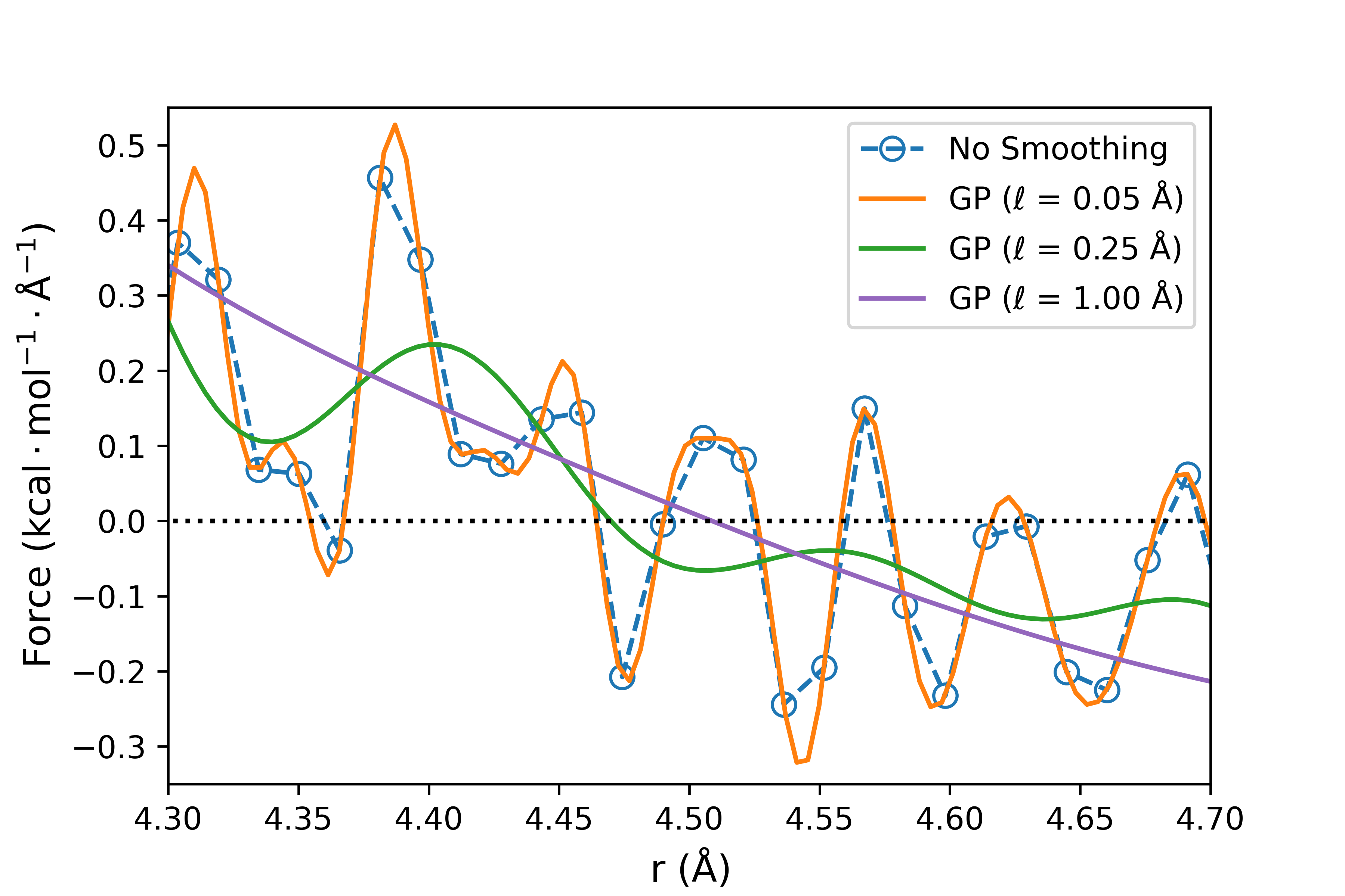
Figure 9: The force calculated from the Xe-274K tabulated potential (blue circles) compared to a non-parametric GP regressed potential at three different length-scale parameters ($\ell$ = 0.05, 0.25, 1.00 Å) (orange, green, and purple line).

The GP regressed structure-optimized potential is then applied in the molecular simulation corrector to calculate a simulated radial distribution function, $g^{(n)}(r^{\prime})$. The molecular simulation corrector is a Canonical ($NVT$) molecular dynamics simulation performed in HOOMD-Blue [110]. MD simulations were initiated with a 500 atom fcc-lattice at the experimental density and equilibrated with Langevin dynamics for $5\times 10^{3}$ timesteps ($dt=5$ femtoseconds). Tabulated structure-optimized potentials were truncated at $3r_{vdW}$ with analytical tail corrections, and simulated radial distribution functions were calculated with MDAnalysis [111, 112] from $1\times 10^{5}$ timestep trajectories sampled at $100$ timestep intervals. Convergence is checked against the average squared error between the simulated and experimental radial distribution function such that $\langle[\Delta g^{(n)}(r^{\prime})]^{2}\rangle<10^{-4}$, which generally is satisfied within 5-10 iterations at scaling constant $\gamma=0.2$.

Table 3: Reduced temperature ($T_{r}=T/T_{c}$) and atomic density ($\rho$) are listed for the neutron scattering experimental conditions. Reference van der Waal radii ($r_{vdW}$) are used to define pair potential truncation in molecular dynamics simulations. $\sigma_{ai}$ is defined as the radius where the quantum dimer pair potential transitions from positive to negative potential energy and $\epsilon_{ai}$ is the potential minimum.

Element	$T_{r}$	$\rho$ (1/Å3)	$r_{vdW}$ (Å)	$\sigma_{ai}$ (Å)	$\epsilon_{ai}$ (kcal/mol)
Ne	0.95	0.02477	2.91	2.76	0.122
Ar	0.56	0.02125	3.55	3.35	0.287
Kr	0.95	0.01187	3.82	3.58	0.582
Xe	0.95	0.00881	4.08	3.89	0.811

Structure-inversion was initiated with a target experimental radial distribution function and a reference (or model) pair potential, $v_{2}^{0}(r_{i})$. Experimental radial distribution data determined with elastic neutron scattering [13, 2, 104] were compiled at the thermodynamic state conditions listed in Table 3. Reference quantum dimer potentials were obtained via couple-cluster theory/t-aug-cc-pV6Z quality basis sets with spin-orbit relativistic corrections. In practice, any of the numerous existing pair potentials for the noble gases may be applied as a reference potential with equivalent outcomes for the structure-optimized potential (see Supporting Information). However, selecting the quantum dimer pair potential as the reference guarantees that the structure-optimized refinement correction is equal to the pairwise many-body contribution to the effective pair potential, $v_{2}^{m}(\mathbf{r}_{ij};\rho,T)=\gamma\beta^{-1}\sum_{n}\Delta g^{(n)}(r^{\prime}_{i})$.

2.5 Supporting Information

2.5.1 Grand Canonical Monte Carlo Simulations

Vapor-liquid coexistence curves and vapor pressures were determined from histogram-reweighting Monte Carlo simulations in the grand canonical ensemble[113, 114, 115]. Simulations were performed with GPU Optimized Monte Carlo (GOMC), version 2.70[83]. All calculations were performed in a cubic cell with a side length of 25 Å. Initial configurations were generated with Packmol [116]. Psfgen was used to generate coordinate (*.pdb) and connectivity (*.psf) files[117]. The Mie potentials were truncated at 10 Å and analytical corrections were applied to the energy and pressure[118]. A hard inner cutoff was used to reject any MC moves that placed atom centers closer than 0.5 Å. A move ratio of 40% displacements and 60% molecule transfers was used. Configurational-bias Monte Carlo (CBMC) was used to improve the acceptance rate for molecule transfers [119]. Three trial locations were used for simulations near the critical temperature, while 8 trial sites were used for the lowest temperature simulations (Tr=0.65). Acceptance rates for molecule insertions in liquid phase simulations were between 0.5% and 6.2%, depending on, chemical potential, and temperature.

To generate the phase diagrams predicted by each parameter set, 9 to 10 simulations were performed; one simulation to bridge the gas and liquid phases near the critical temperature, four in the gas phase, and 5 to 6 liquid simulations. For all noble gases, 2x106 Monte Carlo steps (MCS) were used for equilibration, followed by a data production period of 1.8x107 steps or 4.8x107 steps for gas and liquid phase simulations, respectively. Histogram data were collected as samples of the number of molecules in the simulation cell and the non-bonded energy of the system. Samples were taken on an interval of 500 MCS. Histograms from the GCMC simulations were reweighted and properties calculated as described by Messerly [120]. Averages and statistical uncertainties were determined from five independent sets of simulations, where each simulation was started with a different random number seed. Phase coexistence data for each noble gas is provided in tables 4, 5, 6 and 7 and compared to existing force field models in Figure 10.

2.5.2 Tabulated SOPR Results

Tab-delimited text files (.txt) for experimental radial distribution functions [2, 104, 13] and tabulated structure-optimized potentials obtained in this study are included as supplemental documents. Units for the radial distribution function are in angstrom (Å) in the radius and dimensionless in the g(r). Units for the provided structure-optimized potentials are angstrom (Å) in the radius and kcal/mol in the potential energy.

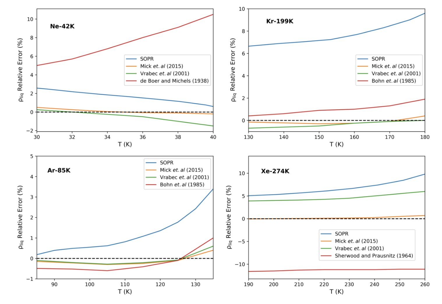
Figure 10: Relative error in liquid density for the noble liquids. Relative error plots were generated with SOPR VLE data and compared to the reported error from other force fields.

Table 4: Phase coexistence data from SOPR Ne-42K potential.

T (K)	$\rho_{liq}$ (kg/m3)	$\rho_{vap}$ (kg/m3)	P (bar)	dHv (kJ/mol)	Z
43	733.714264	256.047536	23.57491	0.655222	0.519732
42	802.903123	211.968635	20.710539	0.809184	0.564664
41	858.831461	173.977971	18.089103	0.94601	0.615533
40	902.873606	144.342911	15.718855	1.057575	0.660804
39	940.575247	120.887088	13.581881	1.150318	0.699232
38	974.392979	101.635719	11.659854	1.230199	0.732772
37	1005.361735	85.477948	9.937776	1.300566	0.762674
36	1034.327748	71.748811	8.402114	1.363704	0.789545
35	1061.845082	59.979902	7.040359	1.421216	0.814005
34	1088.031234	49.834866	5.8411	1.473944	0.836737
33	1113.06391	41.095363	4.79364	1.522527	0.857957
32	1137.482411	33.601697	3.886811	1.567896	0.877381
31	1161.202543	27.203598	3.109184	1.609999	0.894878
30	1183.701132	21.764617	2.45	1.648361	0.910751
29	1205.099967	17.173856	1.898661	1.683608	0.925314
28	1225.73425	13.340107	1.444291	1.716293	0.938529
27	1246.346124	10.178756	1.075976	1.747296	0.950288
26	1267.238749	7.607599	0.782745	1.777414	0.960517
25	1287.667888	5.551135	0.554253	1.806016	0.969351

Table 5: Phase coexistence data from SOPR Ar-85K potential.

T (K)	$\rho_{liq}$ (kg/m3)	$\rho_{vap}$ (kg/m3)	P (bar)	dHv (kJ/mol)	Z
152	798.196968	291.533313	45.571786	2.243789	0.494141
150	836.656053	257.222877	42.268671	2.591589	0.526387
148	874.397214	226.119637	39.149769	2.934793	0.562104
146	908.89679	199.775981	36.212629	3.246104	0.596555
144	939.435052	177.960207	33.447597	3.515884	0.627142
142	966.572627	159.643406	30.843602	3.749191	0.65375
140	991.203415	143.860244	28.391126	3.955419	0.677329
138	1014.0377	129.965504	26.082236	4.142081	0.698752
136	1035.52168	117.564032	23.910432	4.313827	0.718554
134	1055.91477	106.402261	21.869793	4.473382	0.737011
132	1075.37469	96.299118	19.954885	4.62246	0.754289
130	1094.01521	87.114077	18.160762	4.762317	0.770526
128	1111.9393	78.733568	16.482801	4.894038	0.785862
126	1129.25415	71.065144	14.916567	5.01865	0.800437
124	1146.0727	64.035994	13.457917	5.137141	0.814362
122	1162.49057	57.588697	12.10266	5.250322	0.827692
120	1178.56105	51.677614	10.846588	5.358677	0.840417
118	1194.2921	46.262093	9.685515	5.462372	0.852513
116	1209.64317	41.304773	8.615326	5.561308	0.863972
114	1224.53168	36.770416	7.632034	5.65525	0.874829
112	1238.91774	32.627499	6.731743	5.744209	0.885141
110	1252.88688	28.848214	5.910461	5.828782	0.894943
108	1266.59482	25.408149	5.164272	5.909884	0.904268
106	1280.1958	22.28512	4.48897	5.988369	0.913082
104	1293.80881	19.457582	3.880413	6.064929	0.921381
102	1307.41921	16.905474	3.334503	6.139582	0.929153
100	1320.88493	14.609372	2.84726	6.211769	0.936441
98	1334.0903	12.551765	2.414737	6.281104	0.943246
96	1347.00602	10.715882	2.033112	6.347769	0.949619
94	1359.65999	9.086014	1.698543	6.412183	0.955572
92	1372.01604	7.647196	1.407326	6.474152	0.961156

Table 6: Phase coexistence data from SOPR Kr-199K potential.

T (K)	$\rho_{liq}$ (kg/m3)	$\rho_{vap}$ (kg/m3)	P (bar)	dHv (kJ/mol)	Z
210	1531.11817	459.974951	50.626437	3.765603	0.528218
205	1645.79806	366.381497	43.961845	4.596145	0.589887
200	1742.68564	297.413939	37.995176	5.276635	0.64375
195	1825.46461	245.594213	32.649925	5.824705	0.687084
190	1897.63413	204.286876	27.866868	6.283993	0.723559
185	1961.92976	170.227413	23.603813	6.681208	0.75537
180	2021.7309	141.580536	19.823791	7.036668	0.78395
175	2078.16333	117.248277	16.492711	7.359511	0.810074
170	2131.4784	96.538731	13.578873	7.653746	0.833855
165	2181.75136	78.900464	11.051246	7.921878	0.855509
160	2228.9557	63.882448	8.880364	8.166045	0.8756
155	2274.54894	51.154757	7.03666	8.393506	0.894387
150	2320.48457	40.456479	5.488944	8.611949	0.911566
145	2366.20448	31.546962	4.206358	8.819254	0.926747
140	2409.88941	24.20158	3.159392	9.010171	0.93975
135	2451.57431	18.215968	2.319986	9.186547	0.950773
130	2491.53902	13.40713	1.660498	9.350053	0.960133
125	2529.71653	9.614336	1.154729	9.501783	0.968318
120	2566.36151	6.690208	0.777101	9.643374	0.975484
115	2603.29991	4.497391	0.503879	9.781788	0.981806
110	2639.67485	2.90476	0.313072	9.915437	0.9874

Table 7: Phase coexistence data from SOPR Xe-274K potential.

T (K)	$\rho_{liq}$ (kg/m3)	$\rho_{vap}$ (kg/m3)	P (bar)	dHv (kJ/mol)	Z
290	1872.4037	526.262111	52.004613	5.440892	0.538123
285	1967.09269	447.677473	46.976381	6.239123	0.581441
280	2054.03333	382.799284	42.336581	6.963763	0.623764
275	2131.14867	330.772546	38.056685	7.58385	0.660695
270	2199.59475	288.319254	34.106135	8.11039	0.691874
265	2261.17401	252.55593	30.461055	8.56687	0.718742
260	2317.52979	221.658863	27.102719	8.97288	0.742652
255	2370.16211	194.549802	24.015796	9.342204	0.764464
250	2420.26327	170.55061	21.186091	9.684	0.784675
245	2468.44759	149.194894	18.600206	10.003237	0.803583
240	2514.7754	130.143936	16.245757	10.301796	0.821372
235	2559.24147	113.137502	14.110993	10.581039	0.838146
230	2602.16918	97.96734	12.183996	10.843475	0.853924
225	2643.96701	84.455192	10.452821	11.091671	0.86869
220	2684.68136	72.445131	8.905584	11.326431	0.882415
215	2724.1085	61.796925	7.530531	11.547532	0.895084
210	2762.2453	52.38534	6.31611	11.755633	0.906699
205	2799.37292	44.095262	5.25085	11.952533	0.917324
200	2835.94066	36.824133	4.323573	12.140646	0.927067
195	2872.3748	30.47986	3.522885	12.322267	0.935986
190	2908.51521	24.978722	2.837801	12.497539	0.944192
185	2943.61226	20.248163	2.257546	12.663904	0.951618
180	2977.54768	16.217716	1.771668	12.821135	0.958263
175	3011.05962	12.81936	1.369788	12.972135	0.964041
170	3045.27725	9.987163	1.041737	13.121276	0.968718
165	3080.69488	7.655546	0.777787	13.270025	0.972114
160	3115.40577	5.762415	0.568922	13.411029	0.974169
155	3148.6791	4.250562	0.40665	13.544108	0.974402
150	3180.41128	3.065916	0.283242	13.67061	0.97227
145	3207.49035	2.156153	0.191456	13.774698	0.966664
140	3227.16642	1.474877	0.125163	13.840011	0.956789

2.5.3 Convergence Stability

In general, the reference potential can impact the stability of the molecular simulation as well as the interpretation of the structural correction term. In this study, it was possible to directly equate the structure refinement term and the ensemble averaged many-body term since an accurate quantum dimer reference potential was applied. However, if one requires only a structure-optimized potential and not a quantification of the many-body effects, the reference potential can be arbitrarily selected if it is stable within the molecular simulation. For example, Figure 11 shows Xe-274K structure- optimized potentials given five different reference potential conditions; namely, LJ parameters for Ne, Ar, Kr, Xe, and Ra [121, 122]. Clearly, the predicted structure-optimized potential is independent of the reference potential in this system, although in principle this may not hold in complex liquids or for thermodynamic states near the amorphous glass transition where the structure does not explicitly depend on the non-bonded potential energy (e.g. as T$\to$ 0).

In addition to the reference potential, the scaling coefficient defined in Equation (17) can also impact the convergence rate and stability. For example, structure inversion runs for the Xe-274K system at varying scaling coefficient demonstrates that a scaling coefficient of 0.6 is ideal for rapid convergence and low relative deviation from the experimental structure at high iteration number (Figure 12). Therefore, scaling coefficients can significantly impact computational performance and should be optimized for physical systems where molecular simulation is computationally expensive (e.g. high molecular weight liquids).

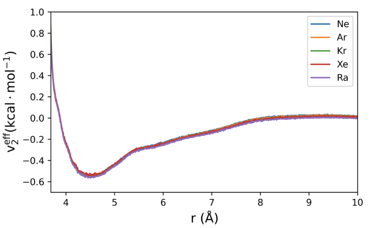
Figure 11: Structure-optimized potentials are unique up to negligible numerical fluctuations for the Xe-274K scattering data given a broad range of reference potentials (LJ parameters for Ne, Ar, Kr, Xe, and Ra).

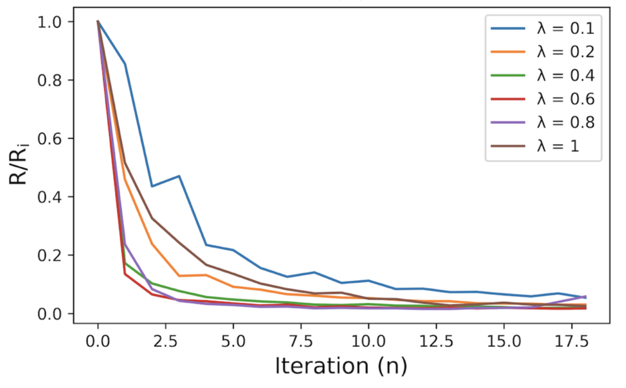
Figure 12: Normalized relative error in the simulated and experimental radial distribution function, defined as the sum-of-square residual (ssr) at iteration n divided by the initial ssr, R/Ri.

2.5.4 Gaussian Process Regression

Gaussian process (GP) regression is a powerful and robust method to perform non-parametric regression of complex functions. One of the main benefits of GP regression is that it has an assumption-free, analytical Fourier transform (FT) that is more accurate than a discrete Fourier transform (DFT) in noise-free and noise-corrupted signals. In fact, it has been shown that conventional DFT is a special case of the more general Bayesian formulation of Fourier transforms that is only possible with a GP regression [109]. With respect to scattering analysis, techniques such as fitting to Poisson series expansions in EPSR and Dissolve simulation packages [123, 75] were implemented since they had analytical FTs that improve the convergence and accuracy of the inverse algorithm. Additionally, GP regression probabilistically smooths the predicted potential, which was shown in the main text to eliminate numerical fluctuations in the interatomic force that can propagate between refinement iterations. Figure 13 shows that structure-optimized potentials in a standard Schommer’s algorithm exhibit sub-angstrom fluctuations near equilibrium separation that are likely caused by the propagation of numerical/experimental noise introduced in the refinement procedure. However, the GP assisted Schommer’s algorithm smooths the potentials so that they adhere more to transferable potential forms while still providing an excellent quality-of- fit to the radial distribution function.

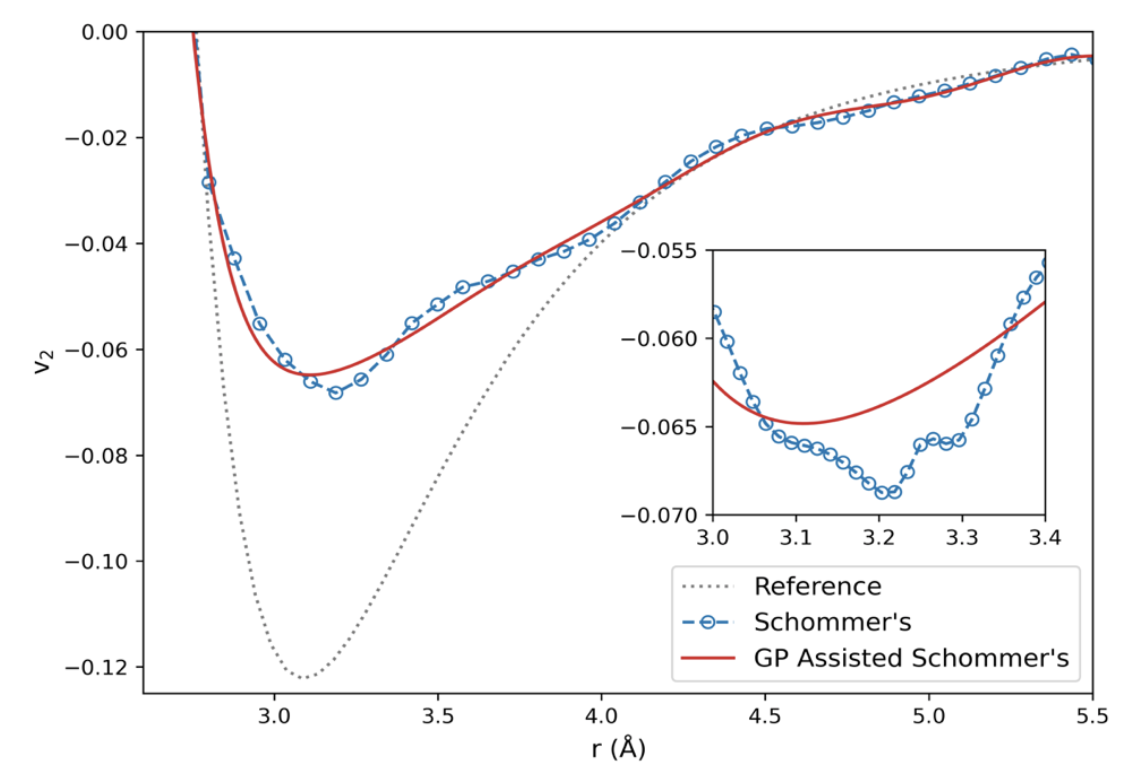
Figure 13: Structure-optimized potentials with and without GP regression.

2.5.5 Triple and Critical Point Structural Many-Body Corrections

SOPR potentials were generated at near triple and critical point conditions for each fluid where scattering data was available (Ne, Kr, and Xe). For each fluid, the dispersion energy decreased with increasing temperature (Figure 14) consistent with the expected increase in exchange repulsion effects, and the repulsive exponent decreased with increasing temperature (Figure 15). The change in the short-range repulsion rate between the near triple and critical point states was found to be negligible in Ne, likely because the difference in absolute temperature is smaller (16 K) compared to the difference in absolute temperature for Kr (69 K) and Xe (105 K). Additionally, inelastic and incoherent scattering corrections have been shown to broaden the radial distribution function in hard spheres [4] resulting in a decrease in both the height and slope of the first solvation shell. Furthermore, post- processing and low instrument resolution for the available scattering data propagate non-negligible error to the determined structure factors which is further confounded by discrete Fourier transform truncation error [74]. While these realities motivate the use of uncertainty quantification in structure inversion, it is likely that new scattering measurements with state-of-the-art neutron instruments must be obtained to draw significant, quantitative conclusions on the many-body corrections.

Figure 14: SOPR potentials for near triple and critical point experimental scattering data.

Figure 15: Repulsive region of the SOPR potentials for Ne, Kr, and Xe.

2.6 Python Notebook Tutorial

In addition to the manuscript, an example code for running SOPR in python was created and posted on GitHub (https://github.com/hoepfnergroup/SOPR). The notebook is reproduced as a pdf below and contains a detailed description of the code functions, basic theory, and results of the method. The example is for liquid neon which is a traditionally challenging liquid to model with molecular dynamics due to its low temperature and significant quantum mechanical effects. The notebook provides relevant background on iterative refinement algorithms, Gaussian process regression, simple liquid molecular simulations in HOOMD-Blue, and visualization of the SOPR results.

See pages 1-11 of sopr_tutorial.pdf

3 Accelerated Bayesian Force Field Uncertainty Quantification for Structural Correlations

The previous chapter explored the estimation of pair interactions from experimental neutron scattering data using Gaussian process (GP) priors conditioned on iterative potential refinement guided by the Henderson inverse theorem. GPs were shown to provide non-parametric interaction potentials with uncertainty quantification, enabling the construction of flexible yet physically-justified pair potentials. However, there are instances where it is desirable to reproduce scattering data as accurately as possible given a parametric potential form. For instance, parametric models are more widely adopted, easily implemented in existing software packages, and are faster to compute than non-parametric potentials. In this case, Bayesian inference over the model parameters can be performed with neutron data as the target quantity-of-interest (QoI).

The main challenge with this approach is not in its construction, but rather the exceptional computational cost of Bayesian inference due to the curse of dimensionality. The main pinch point is that molecular simulations take a long time to perform (ranging from minutes to days) and Bayesian inference necessitates performing thousands to hundreds of thousands of such calculations. In practice, we can alleviate this problem by training machine learning surrogate (or meta-) models on a smaller subset of simulations and then use this surrogate model in place of the more expensive molecular simulation. Some commonly used methods for designing surrogate models include polynomial chaos expansions, neural networks, and GPs.

The built-in uncertainty quantification of GP surrogate models makes them particularly attractive for molecular systems, particularly when the amount of training data is small. GPs excel with little training data because a well-posed prior and kernel function can guide the prediction and enforce physically-justified behavior a priori. Of course, these advantages come with a drawback, namely that the GP evaluation is slow compared to other methods. The content of this chapter is to describe a "greedy" approximation to a GP that provides highly accurate estimations of the molecular model prediction at a fraction of the computational time. In summary, the approximation involves splitting a GP along its independent variable inputs into a subset of GPs, resulting in a reduction in call time-complexity from cubic to linear in the number of independent variables (turning a standard GP into a speedy race car shown in Figure 16). The original publication describing a reliable and robust method for uncertainty quantification and propagation to complex experimental data (i.e. radial distribution functions or electromagnetic spectra) using Bayesian inference is reproduced from the Journal of Chemical Theory and Computation, 2024, 20, 9, 3798–3808 with permission of the publisher. The article is also available on arXiv with article identifier arXiv:2310.19108 [124].

Figure 16: Local Gaussian processes are like a Formula 1 racer in comparison to standard GPs.

3.1 Abstract

While Bayesian inference is the gold standard for uncertainty quantification and propagation, its use within physical chemistry encounters formidable computational barriers. These bottlenecks are magnified for modeling data with many independent variables, such as X-ray/neutron scattering patterns and electromagnetic spectra. To address this challenge, we employ local Gaussian process (LGP) surrogate models to accelerate Bayesian optimization over these complex thermophysical properties. The time-complexity of the LGPs scales linearly in the number of independent variables, in stark contrast to the computationally expensive cubic scaling of conventional Gaussian processes. To illustrate the method, we trained a LGP surrogate model on the radial distribution function of liquid neon and observed a 1,760,000-fold speed-up compared to molecular dynamics simulation, beating a conventional GP by three orders-of-magnitude. We conclude that LGPs are robust and efficient surrogate models, poised to expand the application of Bayesian inference in molecular simulations to a broad spectrum of experimental data.

3.2 Introduction

Molecular simulations are able to estimate a broad array of complex experimental observables, including scattering patterns from neutron and X-ray sources and spectra from near-infrared [125], terahertz [126], sum frequency generation [127, 128], and nuclear magnetic resonance [129]. Recent interest in these experiments to study hydrogen bonding networks of water at interfaces [130, 131], electrolyte solutions [132], and biological systems [133] has motivated the continued advancement of simulations to calculate these properties from first-principles [134, 135, 136]. However, the ability to estimate these complex properties comes with a high computational cost. This barrier greatly limits our ability to quantify how experimental, model, and parametric uncertainty impact molecular simulation predictions, making it difficult to know whether a model is an appropriate representation of nature or if it is simply over-fitting to a given training set. Therefore, what is needed is a computationally efficient and rigorous uncertainty quantification/propagation (UQ/P) method to link molecular models to large and complex experimental datasets.

Bayesian methods are the gold standard for these aims [137], with examples spanning from neutrino and dark matter detection [138], materials discovery and characterization [139, 140, 141, 142], quantum dynamics [143, 144], to molecular simulation [145, 146, 147, 148, 149, 150, 151, 152, 153, 154, 155]. The Bayesian probabilistic framework is a rigorous, systematic approach to quantify probability distribution functions on model parameters and credibility intervals on model predictions, enabling robust and reliable parameter optimization and model selection [39, 156]. Interest in Bayesian methods and uncertainty quantification for molecular simulation has surged [157, 158, 159, 160, 161, 162] due to its flexible and reliable estimation of uncertainty, ability to identify weaknesses or missing physics in molecular models, and systematically quantify the credibility of simulation predictions. Additionally, standard inverse methods including relative entropy minimization, iterative Boltzmann inversion, and force matching have been shown to be approximations to a more general Bayesian field theory [44].

The biggest problem plaguing Bayesian inference is its massive computational cost. The two major pinch points are (1) sampling in high-dimensional spaces, commonly known as the "curse of dimensionality", and (2) the large number of model evaluations required to get accurate uncertainty estimates. In computational chemistry, these bottlenecks are magnified since these models are typically expensive. Therefore, rigorous and accurate uncertainty estimation is challenging, or even impossible, without accelerating the simulation prediction time. One way to achieve this speed-up is by approximating simulation outputs with an inexpensive machine learning model. These so-called surrogate models have been developed from neural networks [153, 163], polynomial chaos expansions [164, 165], configuration-sampling-based methods [166] and Gaussian processes [108, 167, 168].

Gaussian processes (GPs) are a compelling choice as surrogate models thanks to several distinct advantages. GPs are non-parametric, kernel-based function approximators that can interpolate function values in high-dimensional input spaces. GPs with an appropriately selected kernel also have analytical derivatives and Fourier transforms, making them well-suited for physical quantities such as potential energy surfaces [169, 170]. Additionally, kernels can encode physics-informed prior knowledge, alleviating the "black box" nature inherent to many machine learning algorithms. In fact, a comparison of various nonlinear regressors for molecular representations of ground-state electronic properties in organic molecules demonstrated that kernel regressors drastically outperformed other techniques, including convolutional graph neural networks [171].

Perhaps the most widely adopted application of GP surrogate models in computational chemistry is for model optimization. In the last decade, GP surrogates of simple thermophysical properties including density, heat of vaporization, enthalpy, diffusivity and pressure have been used for force field design [172, 173, 174, 175, 176, 177]. However, to our knowledge there are no Bayesian optimization studies that apply GP surrogate models to thermophysical properties with many independent variables, such as structural correlation functions or electromagnetic spectra. In this work, independent variables (IVs) are defined as the fixed quantities over which a measurement is made (e.g. frequencies along a spectrum or radial positions along a radial distribution function) and the outcomes of those measurements are referred to as quantities-of-interest (QoIs).

Measurements of complex QoIs with many IVs are often available or easily obtained, yet are rarely included as observations in Bayesian optimization of molecular models. One reason why this may be the case is that previous literature has not outlined accurate and robust approaches to design Gaussian process surrogates for such data. For example, Angelikopoulous and coworkers did not use GP surrogate models for their Bayesian analysis on the radial distribution function (RDF) of liquid Ar [172], despite the fact that doing so would significantly reduce computation time. It is likely that GPs have not been previously used for complex QoIs due to high training and evaluation costs. Specifically, GPs have a cubic time-complexity in the number of IVs, which quickly becomes prohibitively expensive as experimental measurements obtain higher ranges and resolutions.

Local Gaussian processes (LGPs) are an emerging class of accelerated GP methods that are well-equipped to handle large sets of experimental data. These so-called "greedy" Gaussian process approximations are constructed by separating a GP into a subset of GPs trained at distinct locations in the input space [167, 178, 179, 180]. Computation on the LGP subset scales linearly with the number of IVs, is trivially parallelizable, and easily implemented in high-performance computing (HPC) architectures [181, 182]. State-of-the-art LGP models have been used to design Gaussian approximation potentials (GAPs) [183], a type of machine learning potential used to study atomic [184, 185, 186] and electron structures [187, 183], as well as nuclear magnetic resonance chemical shifts [188] with uncertainty quantification [157]. However, to our knowledge LGPs have not been applied as surrogate models for UQ/P on complex experimental data in computational chemistry.

In this study, we detail a simple and effective surrogate modeling approach for complex experimental observables common in physical chemistry. LGPs unlock the capability for existing Bayesian optimization schemes to incorporate complex data efficiently and accurately at a previously inaccessible computational scale. The key feature of the LGP surrogate model is the reduction in time-complexity with respect to the number of QoIs from cubic to linear, resulting in orders-of-magnitude speed-ups to evaluate complex observable surrogate models and perform posterior estimation. The computational speed-up results from reducing the dimensionality of matrix operations and therefore enables Bayesian UQ/P on experimental data with many IVs. For illustration, consider that a typical Fourier transformed infrared spectroscopy (FT-IR) measurement may contain data between 4000-400 cm^-1 at a resolution of 2 cm^-1, giving a total number of QoIs around $\eta=1800$. According to the time-complexity scaling in $\eta$, a LGP is estimated to accelerate this computation compared to a standard GP by approximately 3,240,000x. Source code and a tutorial on building LGP surrogate models is provided on GitHub.

To demonstrate the method, we trained a LGP surrogate model on the RDF of the ($\lambda$-6) Mie fluid and performed Bayesian optimization to fit the parameters of the Mie fluid model to a neutron scattering derived RDF for liquid neon (Ne). The LGP was found to accelerate the $\eta=73$ independent variable surrogate model calculation approximately 1,760,000x faster than molecular dynamics (MD) and 2100x faster than a conventional GP with accuracy comparable to the uncertainty in the reported experimental data. Bayesian posterior distributions were then calculated with Markov chain Monte Carlo (MCMC) and used to draw conclusions on model behavior, uncertainty, and adequacy. Surprisingly, we find evidence that Bayesian inference conditioned on the radial distribution function significantly constrains the ($\lambda$-6) Mie parameter space, highlighting opportunities to improve force field optimization and design based on neutron scattering experiments.

3.3 Computational Methods

In the following sections, an outline of standard approaches for Bayesian inference and surrogate modeling with Gaussian processes is presented. Then, we describe the local Gaussian process approximation and highlight key differences in their implementation and computational scaling.

3.3.1 Bayesian Inference

Bayes’ law, derived from the definition of conditional probability, is a formal statement of revising one’s prior beliefs based on new observations. Bayes’ theorem for a given model, set of model input parameters, $\boldsymbol{\theta}$, and set of experimental QoIs, $\mathbf{y}$, is expressed as,

$$p(\boldsymbol{\theta}|\mathbf{y})\propto p(\mathbf{y}|\boldsymbol{\theta})p(\boldsymbol{\theta})$$ (21)

where $p(\boldsymbol{\theta})$ is the ’prior’ probability distribution over the model parameters, $p(\mathbf{y}|\boldsymbol{\theta})$ is the ’likelihood’ of observing $\mathbf{y}$ given parameters $\boldsymbol{\theta}$, and $p(\boldsymbol{\theta}|\mathbf{y})$ is the ’posterior’ probability that the underlying parameter $\boldsymbol{\theta}$ models or explains the observation $\mathbf{y}$. Equality holds in Eq. (21) if the right-hand-side is normalized by the ’marginal likelihood’, $p(\mathbf{y})$, but including this term explicitly is unnecessary since the posterior probability distribution can be normalized post hoc. In molecular simulations, $\boldsymbol{\theta}$ is the set of unknown parameters in the selected model, usually the force field parameters in the Hamiltonian, to the experimental QoI that the simulation estimates. The observations, $\mathbf{y}$, can be any QoI or combination of QoIs (e.g. RDFs, spectra, densities, diffusivities, etc). This construction, known as the standard Bayesian scheme, is generalizable to any physical model and its corresponding parameters including density functional theory (DFT), ab initio molecular dynamics (AIMD), and path integral molecular dynamics (PIMD).

Calculating the posterior distribution then just requires prescription of prior distributions on the model input parameters and evaluation of the likelihood function. In this work, Gaussian distributions are used for both the prior and likelihood functions, which is a standard choice according to the central limit theorem. The Gaussian likelihood has the form,

$$p(\mathbf{y}|\boldsymbol{\theta})=\bigg{(}\frac{1}{\sqrt{2\pi}\sigma_{n}}\bigg{)}^{\eta}\exp[-\frac{1}{2\sigma_{n}^{2}}\sum_{i=1}^{\eta}\ [\mathbf{y}_{\boldsymbol{\theta}}-\mathbf{y}]^{2}\bigg{]}$$ (22)

where $\eta$ is the number of observables in $\mathbf{y}$, $\mathbf{y}_{\boldsymbol{\theta}}$ is the model predicted observables at model input $\boldsymbol{\theta}$, and $\sigma_{n}$ is a nuisance parameter describing the unknown variance of the Gaussian likelihood. Cailliez and coworkers choose the nuisance parameter as the sum of simulation and experiment variances ($\sigma_{n}^{2}\approx\sigma_{sim}^{2}+\sigma_{exp}^{2}$) [173]; however, if these variances are unknown or one wishes to explore the distribution of variances, the nuisance parameter can be inferred via the Bayesian inference. Hence, the resulting posterior distribution on the nuisance parameter includes the unknown uncertainty arising due to the sum of the model and the experimental variances. In this work, the nuisance parameter is treated as an unknown to be inferred along with the explicit model parameters. Note that in some cases a different likelihood function may be more appropriate based on physics-informed prior knowledge of the distribution of the observable of interest (e.g. the multinomial likelihood in relative entropy minimization between canonical ensembles [24]).

The computationally expensive part of calculating Eq. 22 is determining $\mathbf{y}_{\boldsymbol{\theta}}$ at a sufficient number of points in the parameter space. Generally, this can be achieved by calculating $\mathbf{y}_{\boldsymbol{\theta}}$ at dense, equally spaced points in the parameter space of interest (grid method), sampling the parameter space with Markov chain Monte Carlo (MCMC) to estimate the posterior with a histogram (approximate sampling method), or assuming that the posterior distribution has a specific functional form (i.e. Laplace approximation). Regardless of the selected method, each of these posterior distribution characterization techniques require a prohibitive number of molecular simulations to adequately sample the parameter space (often on the order of $10^{5}-10^{6}$), which is infeasible for even modest sized molecular systems.

3.3.2 Gaussian Process Surrogate Models

Gaussian processes accelerate the Bayesian likelihood evaluation by approximating $\mathbf{y}_{\boldsymbol{\theta}}$ with an inexpensive matrix calculation. A Gaussian process is a stochastic process such that every finite set of random variables (position, time, etc) has a multivariate normal distribution [108]. The joint distribution over all random variables in the system therefore defines a functional probability distribution. The expectation of this distribution maps a set of model parameters, $\boldsymbol{\theta}^{*}$, and IVs, $\mathbf{r}$, to the most probable QoI given the model parameters, $S(\mathbf{r}|\boldsymbol{\theta}^{*})$, such that,

$$\mathbb{E}[GP]:\boldsymbol{\theta}^{*}\times\mathbf{r}\mapsto S(\mathbf{r}|\boldsymbol{\theta}^{*})$$ (23)

where the expectation operator is written in terms of a kernel matrix, $\mathbf{K}$, training set parameter matrix, $\mathbf{\hat{X}}$, and training set output matrix, $\mathbf{\hat{Y}}$, according to the equation,

$$\mathbb{E}[\textit{GP}(\boldsymbol{\theta}^{*},\mathbf{r})]=\mathbf{K}_{(\boldsymbol{\theta}^{*},\mathbf{r}),\mathbf{\hat{X}}}[\mathbf{K}_{\mathbf{\hat{X}},\mathbf{\hat{X}}}+\sigma_{noise}^{2}\mathbf{I}]^{-1}\mathbf{\hat{Y}}$$ (24)

where $\sigma_{noise}^{2}$ is the variance due to noise and $\mathbf{I}$ is the identity matrix. Note that in general the IVs, $\mathbf{r}$, can be multidimensional. As an example, consider the case a GP maps a set of force field parameters to the angular RDF of a liquid. We now have a 2-dimensional space of IVs since the angular RDF gives the atomic density along the radial and angular dimensions. In the following mathematical development, it is assumed that the QoI is 1-dimensional for sake of convenience and note that extending the method to higher-dimensional observables just requires redefining the IVs in accordance with Eq. (24).

The kernel matrix, $\mathbf{K}$, quantifies the relatedness between input parameters and can be selected based on prior knowledge of the physical system. A standard kernel for physics-based applications is the squared-exponential (or radial basis function) since the resulting GP is infinitely differentiable, smooth, continuous, and has an analytical Fourier transform [109]. The squared-exponential kernel function between input points $(\boldsymbol{\theta}_{m},r_{m})$ and $(\boldsymbol{\theta}_{n},r_{n})$ is given by,

$$K_{mn}=\alpha^{2}\exp\bigg(-\frac{(r_{m}-r_{n})^{2}}{2\ell_{r}^{2}}-\sum_{o=1}^{\text{dim}(\boldsymbol{\theta})}\frac{(\theta_{o,m}-\theta_{o,n})^{2}}{2\ell_{\theta_{o}}^{2}}\bigg{missing})$$ (25)

where $o$ indexes over dim($\boldsymbol{\theta}$) and the hyperparameters $\alpha^{2}$ and $\ell_{A}$ are the kernel variance and correlation length scale of parameter $A$, respectively. Hyperparameter optimization can be performed by log marginal likelihood maximization, $k$-fold cross validation [108] or marginalization with an integrated acquisition function [189], but can be computationally expensive and is usually avoided if accurate estimates of the hyperparameters can be made from prior knowledge of the chemical system.

To train a standard GP surrogate model, $N$ training samples are generated in the input parameter space and a molecular simulation is performed for each training set sample to calculate $N$ predictions over the number of target QoIs, $\eta$. The training set, $\mathbf{\hat{X}}$, is then a ($N\eta$ $\times$ dim($\boldsymbol{\theta}$) + 1) matrix of the following form,

$$\mathbf{\hat{X}}=\begin{bmatrix}\theta_{1,1}&\theta_{2,1}&\ldots&r_{1}\\ \theta_{1,1}&\theta_{2,1}&\ldots&r_{2}\\ \vdots&\vdots&\vdots&\vdots\\ \theta_{1,1}&\theta_{2,1}&\ldots&r_{\eta}\\ \theta_{1,2}&\theta_{2,2}&\ldots&r_{1}\\ \vdots&\vdots&\vdots&\vdots\\ \theta_{1,N}&\theta_{2,N}&\ldots&r_{\eta}\\ \end{bmatrix}$$ (26)

where the $\theta_{i,j}$ are the $i^{th}$ model parameter for sample index $j$ and $r_{k}$ are the IVs of the target QoI. Note that the training sample index, $j=1,...,N$, is updated in the model parameters only after $\eta$ rows spanning the domain of the observable, giving $N\eta$ total rows. Therefore, the training set matrix represents all possible combinations of the training parameters in the $\boldsymbol{\theta}$ parameter input space. The training set observations, $\mathbf{\hat{Y}}$, are a ($N\eta$ $\times$ 1) column vector of the observable outputs from the training set,

$$\mathbf{\hat{Y}}=[S(\boldsymbol{\theta}_{1},r_{1}),...,S(\boldsymbol{\theta}_{1},r_{\eta}),S(\boldsymbol{\theta}_{2},r_{1}),...,S(\boldsymbol{\theta}_{N},r_{\eta})]^{T}$$ (27)

where $S(\boldsymbol{\theta}_{j},r_{k})=y(\boldsymbol{\theta}_{j},r_{k})-\mu_{GP}^{prior}(\boldsymbol{\theta}_{j},r_{k})$ is the difference between the training set observation of model parameters $\theta_{j}$ at IV $r_{k}$ and a GP prior mean function. Of course, the GP prior mean, $\boldsymbol{\mu}_{GP}^{prior}$, is the same shape as the training set observations matrix,

$$\boldsymbol{\mu}_{GP}^{prior}:=[\mu(\boldsymbol{\theta}_{1},r_{1}),...,\mu(\boldsymbol{\theta}_{1},r_{\eta}),\mu(\boldsymbol{\theta}_{2},r_{1}),...,\mu(\boldsymbol{\theta}_{N},r_{\eta})]^{T}$$ (28)

where $\mu(\boldsymbol{\theta}_{j},r_{k})$ is the GP prior mean for parameter set $\boldsymbol{\theta}_{j}$ at $r_{k}$. Note that the selection of a prior mean can impact the quality of fit of the GP surrogate model and should reflect physically justified prior knowledge of the physical system.

Conceptually, since a Gaussian process is a Bayesian model, the prior serves as a current state of knowledge that can encode an initial guess for the QoI before the GP sees any training data. The subtraction of the GP prior mean from the model output effectively shifts the QoI by this pre-specified mean function. Hence, the GP is trained on these mean shifted observations rather than the observations themselves. Although shifting the data by another function seems like it shouldn’t change the ability of the GP to estimate the QoI, it actually can have an important impact on the stochastic properties of the data as a function of the IVs. By construction, GPs are stationary, meaning that the means, variances, and covariances are assumed to be equal along all QoI. But for complex data, this is often not the case. For example, it is known that the RDF is zero for small $r$ values and has asymptotic tailing behavior to unity at long-range. The GP prior mean effectively shifts this non-stationary data and makes it behave as if it were stationary by removing any $r$ dependencies.

The expectation of the GP for a new set of parameters, $S^{*}(\mathbf{r}|\boldsymbol{\theta}^{*})$, is then a ($\eta$ x 1) column vector calculated with Eq. (24),

$$S^{*}(\mathbf{r}|\boldsymbol{\theta}^{*})=[S^{*}(r_{1}|\boldsymbol{\theta}^{*}),...,S^{*}(r_{\eta}|\boldsymbol{\theta}^{*})]^{T}$$ (29)

where $S^{*}(\mathbf{r}|\boldsymbol{\theta}^{*})$ is the most probable difference function between the model and GP prior mean. Hence, to obtain a comparison to the experimental QoI you simply add the GP prior mean at $\boldsymbol{\theta}^{*}$, $\boldsymbol{\mu}_{GP}^{*,prior}(\mathbf{r}|\boldsymbol{\theta}^{*})$, back to $S^{*}(\boldsymbol{\theta}^{*},\mathbf{r})$.

The GP expectation calculation is burdened by the inversion of the training-training kernel matrix with $\mathcal{O}(N^{3}\eta^{3})$ time complexity and the ($\eta$ $\times$ $N\eta$) $\times$ ($N\eta$ $\times$ $N\eta$) $\times$ ($N\eta$ $\times$ 1) matrix product with $\mathcal{O}(N^{2}\eta^{3})$ time complexity. Note that these estimates are for naive matrix multiplication. Regardless, the cubic scaling in $\eta$ dominates the time-complexity for observables with many QoIs. For example, to build a GP surrogate model for the density of a noble gas ($\eta=1$) with Lennard-Jones interactions (dim($\boldsymbol{\theta}$) = 2) would give a training set matrix of ($2N\times 3)$. Similarly, a surrogate model for an infrared spectrum of water from 600-4000 cm^-1 at a resolution of $4$ cm^-1 ($\eta=850$) estimated with a 3 point water model of Lennard-Jones type interactions (dim($\boldsymbol{\theta}$) = 6) would generate a training set matrix of size (850$N$ $\times$ 7). Clearly, the complexity of the output QoI causes a significant increase in the computational cost of the matrix operations.

3.3.3 The Local Gaussian Process Surrogate Model

The time-complexity of the training-kernel matrix inversion and the matrix product can be substantially reduced by fragmenting the full Gaussian process of Eq. (24) into $\eta$ Gaussian processes. This method is also referred to as the subset of regressors approximation [190] and is considered a "greedy" approximation [108]. Under this construction, an individual $GP_{k}$ is trained to map a set of model parameters to an individual QoI,

$$\mathbb{E}[GP_{k}]:\boldsymbol{\theta}\mapsto S(r_{k})$$ (30)

where $\mathbf{r}$ is no longer an input parameter. The training set matrix, $\mathbf{\hat{X^{\prime}}}$, is now a ($N$ $\times$ dim($\boldsymbol{\theta}$)) matrix,

$$\mathbf{\hat{X^{\prime}}}=\begin{bmatrix}\theta_{1,1}&\theta_{2,1}&\ldots\\ \theta_{1,2}&\theta_{2,2}&\ldots\\ \vdots&\vdots&\vdots\\ \theta_{1,N}&\theta_{2,N}&\ldots\\ \end{bmatrix}$$ (31)

while the training set observations, $\mathbf{\hat{Y^{\prime}}}_{k}$, is a ($N$ $\times$ 1) column vector of the QoIs from the training set at $r_{k}$,

$$\mathbf{\hat{Y}^{\prime}}_{k}=[S(\boldsymbol{\theta}_{1},r_{k}),...,S(\boldsymbol{\theta}_{N},r_{k})]^{T}$$ (32)

where $S(\boldsymbol{\theta}_{j},r_{k})=y(\boldsymbol{\theta}_{j},r_{k})-\boldsymbol{\mu}_{LGP,k}^{prior}(r_{k})$ and $k$ indexes over IVs. The LGP prior mean $\boldsymbol{\mu}_{LGP,k}^{prior}(r_{k})$ is now,

$$\boldsymbol{\mu}_{LGP,k}^{prior}:=[\mu(\boldsymbol{\theta}_{1},r_{k}),...,\mu(\boldsymbol{\theta}_{N},r_{k})]^{T}$$ (33)

such that $\mu(\boldsymbol{\theta}_{j},r_{k})$ is the GP prior mean for parameter $\boldsymbol{\theta}_{j}$ at $r_{k}$. The squared-exponential kernel function is now,

$$K_{mn}=\alpha^{2}\exp\bigg(-\sum_{o=1}^{\text{dim}(\boldsymbol{\theta})}\frac{(\theta_{o,m}-\theta_{o,n})^{2}}{2\ell_{\theta_{o}}^{2}}\bigg{missing}).$$ (34)

The LGP surrogate model expectation for the observable at $r_{k}$, at a new set of parameters, $\boldsymbol{\theta}^{*}$, is just the expectation of the $k^{th}$ Gaussian process given the training set data,

$$S_{loc}^{*}(r_{k}|\boldsymbol{\theta}^{*})=\mathbb{E}[\textit{GP}_{k}(\boldsymbol{\theta}^{*})]=\mathbf{K}_{\boldsymbol{\theta}^{*},\mathbf{\hat{X^{\prime}}}}[\mathbf{K}_{\mathbf{\hat{X^{\prime}}},\mathbf{\hat{X^{\prime}}}}+\sigma_{noise}^{2}\mathbf{I}]^{-1}\mathbf{\hat{Y^{\prime}}}_{k}.$$ (35)

We then just combine the local results from the subset of $\eta$ GPs to obtain a prediction for the difference between the model and LGP prior mean,

$$S_{loc}^{*}(\mathbf{r}|\boldsymbol{\theta}^{*})=[S_{loc}^{*}(r_{1}|\boldsymbol{\theta}^{*}),...,S_{loc}^{*}(r_{\eta}|\boldsymbol{\theta}^{*})]^{T}.$$ (36)

and subsequently add back the LGP prior mean to obtain the estimated QoI, $y_{loc}^{*}(\mathbf{r}|\boldsymbol{\theta}^{*})=S_{loc}^{*}(\mathbf{r}|\boldsymbol{\theta}^{*})+\boldsymbol{\mu}_{LGP,k}^{prior}(\boldsymbol{\theta}^{*},\mathbf{r})$.

By reducing the dimensionality of the relevant matrices, the time complexity of the matrix calculations are drastically reduced compared to a standard GP. The single step inversion of the training-training kernel matrix is now of $\mathcal{O}(N^{3})$ time complexity while the $\eta$ step (1 $\times$ $N$) $\times$ ($N$ $\times$ $N$) $\times$ ($N$ $\times$ 1) matrix products are reduced to $\mathcal{O}(N^{2}\eta)$ time complexity. If the number of training samples, $N$, the number of IVs, $\eta$, and the number of model evaluations, $G$, are equal between the full and LGP algorithms, then a LGP approximation reduces the evaluation time complexity in a standard GP from cubic-scaling, $\eta^{3}$, to embarrassingly parallelizable linear-scaling, $\eta$.

In summary, a local Gaussian process is an approximation in which the QoIs are modeled as independent random variables, each described by their own Gaussian process. This amounts to assuming that the random variables are stochastically independent. For time-independent data including scattering measurements and spectroscopy, this approximation is appropriate since each observation is an independent measurement at each independent variable. Finally, it is well-established that low rank approximations of Gaussian processes can compromise the accuracy of the estimated uncertainty, so the use of LGP regressors should be carefully scrutinized based on the risk/consequences of misrepresenting the resulting functional distributions.

Complex experimental observables can be reconstructed by this set of LGPs through a series of relatively straightforward matrix operations with linear time-complexity in the number of IVs. Furthermore, the LGP has all of the primary advantages of Bayesian methods, including built-in UQ and analytical derivatives and Fourier transforms. In the following section, we demonstrate the computational enhancement and accuracy of the LGP approach by modeling the RDF of neon at 42$K$. The LGP surrogate model is then implemented within a Bayesian framework to exemplify the power of UQ/P for molecular modeling.

3.4 A Local Gaussian Process Surrogate for the RDF of Liquid Ne

To explore the computational advantages of LGP surrogate models for Bayesian inference, we studied the experimental RDF of liquid Ne [13] under a ($\lambda$-6) Mie fluid model. The ($\lambda$-6) Mie force field is a flexible Lennard-Jones type potential with variable repulsive exponent,

$$v^{Mie}_{2}(r)=\frac{\lambda}{\lambda-6}\bigg{(}\frac{\lambda}{6}\bigg{)}^{\frac{6}{\lambda-6}}\epsilon\bigg{[}\bigg{(}\frac{\sigma}{r}\bigg{)}^{\lambda}-\bigg{(}\frac{\sigma}{r}\bigg{)}^{6}\bigg{]}$$ (37)

where $\lambda$ is the short-range repulsion exponent, $\sigma$ is the collision diameter (Å), and $\epsilon$ is the dispersion energy (kcal/mol) [82].

MD simulations were performed from a Sobol sampled set spanning a prior range based on existing force field models [85, 89, 191] ($\lambda=[6.1,18]$, $\sigma=[0.88,3.32]$, and $\epsilon=[0,0.136]$) to generate a RDF training set matrix of the form in Eq. 31. Prior parameter ranges were selected so that training samples were restricted to the liquid regime of the ($\lambda$-6) Mie phase diagram [88, 192]. A sequential sampling approach was used in which we Sobol sample the prior range of parameters, calculate the training sample with the best-fit to the experimental data (lowest root mean squared error), center the new space on this training sample, and then narrow the sample range around this center point by a user selected ratio $\gamma$. This procedure was repeated three times with 320 samples per round (960 total training simulations) with $\gamma=0.8$. This ratio was selected so that the final range would span >3 standard deviations of the posterior distributions estimated in prior literature [172, 89]. Subsequently, 320 test simulations were randomly sampled from the final range and used to determine whether or not the surrogate model provides accurate model predictions. A visualization of this procedure is provided in the Supporting Information.

The number of observed points $\eta$ in the radial distribution function was calculated by dividing the reported $r_{max}-r_{min}\approx 15.3$ by the effective $r$-space resolution given by, $\Delta r=\pi/Q_{max}$, where $\Delta r=0.21$ Åfor reported $Q_{max}=15$ Å^-1. This relation indicates that the appropriate number of observed independent $r$-values in the RDF is $\eta=73$.

The training set matrix and training observation matrix were then constructed from the 960 training samples according to eqs (31) and (32), respectively. As a prior mean, we selected the RDF determined analytically from the dilute limit potential of mean force (PMF),

$$\boldsymbol{\mu}_{PMF,k}^{prior}(\boldsymbol{\theta}_{j},r_{k}):=g(\boldsymbol{\theta}_{j},r_{k})=\exp{[-\beta V(\boldsymbol{\theta}_{j},r_{k})]}$$ (38)

where $g(\boldsymbol{\theta}_{j},r_{k})$ and $V(\boldsymbol{\theta}_{j},r_{k})$ are the analytical dilute limit RDF and ($\lambda$-6) Mie potential for parameters $\boldsymbol{\theta}_{j}$ at $r_{k}$, respectively. A PMF prior mean yields physically realistic short-range ($g(r)=0$) and long-range behavior ($g(r)\to 1$). The PMF prior had improved RMSE compared to an ideal gas prior ($\forall r\in\mathbb{R}_{0}^{+}$, $g(r)=1$), but this difference did not significantly impact the Bayesian posterior estimate (see Supporting Information). Finally, LGP hyperparameter optimization was performed using brute force to minimize the LOO error [193] over the training set.

Quantitative analysis of model sensitivity can be performed with probabilistic derivatives of the QoI with respect to model parameters (see Supporting Information) and subsequently related to temperature derivatives of radial distribution functions [194].

3.4.1 Computational Efficiency and Accuracy

Now that we have constructed the training set matrix, we simply evaluate the expectation at each $r_{k}$ according to Eq. (35) and combine the results into a single array as in Eq. (36). The average computational time to invert the training set matrix and evaluate the surrogate model for both a standard GP and LGP are shown in Table 8. The LGP surrogate accelerates the RDF evaluation time compared to molecular dynamics by a factor of 1,700,000 for the $\eta=73$ independent variable QoI with 960 training simulations. This 6 orders-of-magnitude speed-up beats a standard GP by 3 orders-of-magnitude (2141x). With respect to the training-training kernel matrix inversion, the LGP wins out on the standard GP by a factor of 31,565.

Table 8: Average relative time and speed-up to QoI evaluation and training set matrix inversion for a standard and local Gaussian process for 960 training samples and a RDF with $\eta=73$ points.

Model	QoI Eval. Time (s)	Speed Up ($t/t_{sim}$)	Inv. Time (s)
Simulation	1,251	1	-
GP	1.52	822	355
LGP	0.0007	1,760,267	0.01

In summary, the LGP significantly accelerates both computational bottlenecks for Gaussian process surrogate modeling; namely, the training set matrix inversion and surrogate model evaluation time. Of course, the exact speed-ups depend on numerous factors including the number of IVs $\eta$, the number of training samples used to construct the training set matrix $N$, the level of code parallelization, and hyperparameter optimization procedure. Which step is rate limiting depends on the surrogate modeling application. For instance, if the surrogate model doesn’t need to be evaluated a large number of times, the training set generation, matrix inversion and hyperparameter optimization will be the rate limiting steps. On the other hand, applications that require a large number of model evaluations, such as uncertainty quantification and propagation, result in the surrogate model evaluation time being rate limiting. Typically, designing a surrogate model is only necessary in the latter case.

Clearly the LGP is fast, but is it accurate? In other words, does the LGP provide QoI predictions that are within a reasonable level of accuracy to serve as a true surrogate model for the molecular dynamics predictions? To evaluate the accuracy of the local predictions, a test set of 320 ($\lambda$-6) Mie parameters was randomly sampled from the final range of the sequential sampling method (see Supporting Information) and the RMSE computed between simulated and LGP predicted radial distribution functions along all radial positions, $r$. The results are summarized in Figure 17.

Figure 17: Visualization of LGP surrogate model testing and validation. (a)-(c) Test set samples over each parameter plotted against the RMSE between simulated and LGP data. (d) Average RMSE over the 320 test set samples as a function of $r$. The dashed line represents the reported error from the experiment.

The RMSE for all radial positions is less than 0.03, which is excellent considering that this error is smaller than the reported experimental uncertainty ($\sim$0.03). Of course, the acceptable RMSE over the QoI is user-defined and largely subjective based on the surrogate model application, but can be improved with additional training and hyperparameter optimization if necessary (an example is included in the Supporting Information).

3.4.2 Learning from the Ne RDF Surrogate Model with Bayesian Analysis

Our fast and accurate LGP surrogate model now allows us to explore the underlying probability distributions on the ($\lambda$-6) Mie parameter space. This example is provided to show how one can use Bayesian analysis to learn about correlations and relationships between model parameters as well as model adequacy. This analysis can provide robust insight into the nature of the model and provide quantifiable evidence for whether or not the model is appropriate for a target application. Bayesian inference yields a probability distribution function over the model parameters called the joint posterior probability distribution. The maximum of the joint posterior, referred to as the maximum a posteriori (MAP), represents the set of parameters with the highest probability of explaining the given experimental data. In force field design, the MAP would be an appropriate choice for an optimal set of model parameters. However, the power of the Bayesian approach lies in the fact that, not only can we identify the optimal parameters, but we can also examine the probability distribution of the parameters around these optima. For instance, the width of the distribution provides evidence for how important a parameter in the model is for representing the target data. For a given parameter, a wide distribution indicates that the parameter has little influence on the model prediction. On the other hand, a narrow distribution indicates that the parameter is critical to the model prediction. Additionally, the joint posterior may exhibit multiple peaks, or modes. A multimodal joint posterior suggests that there are multiple sets of model parameters that reproduce the target data, which may be a symptom of model inadequacy. Finally, the symmetry of the distribution provides information on relationships and correlations between parameters, providing a framework to diagnose subtle relationships that may otherwise go unnoticed.

Usually, the joint posterior distribution is a high-dimensional quantity that cannot be visualized directly. However, we can visualize the joint posterior along one dimension by integrating out the contributions over all other parameters. The resulting distributions are called marginal distributions. Marginal distributions computed over the ($\lambda$-6) Mie potential parameters optimized to the RDF of liquid Ne are shown in Figure 18.

Figure 18: (Diagonal) 1D marginal distributions for the ($\lambda$-6) Mie fluid parameters. Prior distributions are not depicted since they are flat lines near 0 probability. Yellow vertical lines represent the maximum a posterior (MAP) estimate. (Off-Diagonal) 2D marginal histograms showing parameter correlations.

For each parameter, the resulting marginal posterior distributions are unimodal and symmetric. This result is not surprising in the context of recent results that show iterative Boltzmann inversion, which is a maximum likelihood approach to the structural inverse problem, is convex for Lennard-Jones type fluids [25]. Observing the 2D marginal distributions in Figure 18, we can also see that each of the parameters are correlated to one other. For example, the negative correlation between $\sigma$ and $\epsilon$ suggests that increasing the size of the particle should be accompanied by a decrease in the effective particle attraction. Conceptually this makes sense, if the particles are larger, then they would need to have a weaker attractive force to give the same atomic structure. This result is consistent with Bayesian analysis on liquid Ar [172]. The nuisance parameter distribution shows that the unknown standard deviation between the LGP surrogate model and the experimental data is around 0.016.

One surprising characteristic of the posterior distribution is that it is extremely narrow. Recall that narrow distributions indicate that the parameters are important, or have tight control, over the model quality-of-fit to the experimental data. From our Bayesian analysis, we can therefore confidently conclude that detailed interatomic force information is contained within the experimental RDF. This observation is in stark contrast to over 60 years of prior literature which has unanimously asserted that only the excluded volume or collision diameter can be ascertained from experimental scattering data [195, 196, 17]. In fact, the Bayesian analysis shows that it is possible to determine values for $\lambda$, $\sigma$, and $\epsilon$ within $\pm 2$, $\pm 0.02$ Å, and $\pm 0.0075$ kcal/mol with 95% certainty. This result leads to two important conclusions: (1) Scattering data can effectively constrain the force field model parameter space and (2) the data must be sufficiently accurate to do so. These results provide evidence that scattering data could be invaluable to inform accurate force fields, particularly for structure and self-assembly applications.

The joint posterior can also be used for model parameter selection given the experimental observation. Specifically, the optimal parameters are given by the MAP, corresponding to the maximum of the joint posterior distribution. The MAP is presented in Table 9 along with two other existing force fields for liquid Ne.

Table 9: Summary of ($\lambda-6)$ Mie potential parameters optimized for Ne. Values for the repulsive exponent parameter are rounded to the nearest integer.

Force Field	QoI	$\lambda$	$\sigma$ (Å)	$\epsilon$ (kcal/mol)
Mick (2015)	VLE	11	2.794	0.064
SOPR (2022)	RDF	11	2.778	0.063
This Work	RDF	11	2.773	0.064

The estimated Mie parameters are in agreement with the Mick [89] and structure optimized potential refinement (SOPR) [191] models. This result confirms that the radial distribution function contains sufficient information to determine transferable force field parameters in simple liquids.

Some interesting questions arise considering that both the Mie fluid model and SOPR, which is a probabilistic iterative Boltzmann method for experimental scattering data, give similar predictions for the structure-optimized potentials. The key difference between the Bayesian optimization performed in this work and SOPR is that the former is parametric while the latter is non-parametric, both of which have strengths and weaknesses. Specifically, parametric models are less complex but may not be flexible enough to describe subtle details of the experimental observation. On the other hand, non-parametric models can describe nuanced experiments but may over-fit to non-physical features of the data. It is then natural to wonder: Is a ($\lambda$-6) Mie model adequate to describe the experimental scattering data? Or does the scattering data complexity necessitate the use of non-parametric iterative potential refinement techniques like SOPR?

We can investigate the first question of model adequacy by propagating parameter uncertainty through the LGP to construct a distribution of RDF predictions - referred to as the posterior predictive. The posterior predictive can be estimated by evaluating the LGP for all MCMC samples and computing the mean,

$$\mathbb{E}[{S}_{loc}^{*}(\mathbf{r}_{k})]\approx\frac{1}{N}\sum_{i=1}^{N}{S}_{loc}^{*}(\mathbf{r}_{k}|\boldsymbol{\theta}_{i})$$ (39)

and variance,

$$\mathbb{V}[{S}_{loc}^{*}(\mathbf{r}_{k})]\approx\frac{1}{N}\sum_{i=1}^{N}({S}_{loc}^{*}(\mathbf{r}_{k}|\boldsymbol{\theta}_{i})-\mathbb{E}[{S}_{loc}^{*}(\mathbf{r}_{k})])^{2}$$ (40)

of the resulting QoI predictions. Recall that the nuisance parameter distribution is also sampled to account for unknown uncertainties in the LGP surrogate model and experimental data. The posterior predictive therefore quantifies of how accurately we know the QoI given experimental, model, and parametric uncertainty estimated with Bayesian inference. If the model is adequate, the Bayesian credibility interval ($\mu\pm 2\sigma$) should contain approximately 95% of the experimental data. The posterior predictive and residuals ($g_{exp}(r)-\mu(r)$) estimated for the liquid Ne RDF are shown in Figure 19.

Figure 19: Posterior predictive plots for the radial distribution function. (a) RDF mean and credibility interval propagated from the parameter uncertainty quantified with Bayesian inference. (b) Residual analysis comparing the experimental data with the posterior predictive distribution.

Clearly, the agreement between the posterior predictive mean and the experimental data is excellent. However, the residuals often lie outside of the $2\sigma_{post}$ credibility interval. These differences between the experiment and model could be explained by a number of different factors, including errors arising from Fourier transform truncation, background scattering corrections or model inadequacy, among others. However, without rigorous uncertainty quantification on the experimental scattering data, it is currently not possible to determine which factor or combination of factors results in the model disagreement. We argue that this knowledge gap necessitates rigorous UQ/P studies on scattering data as well as iterative potential refinement methods. Combining these approaches with Bayesian inference on molecular dynamics models could then shed light on what physical interactions can be learned from scattering experiments.

In summary, we have shown that a LGP surrogate model enables rapid and accurate uncertainty quantification and propagation with Bayesian inference. We then showed how the posterior distribution is an indispensable tool to learn subtle relationships between model parameters, identify how important each model parameter is to describe the outcome of experiments, and quantify our degree of belief that our model adequately describes our observations. The power of Bayesian inference is evident.

3.5 Conclusions

We have shown that local Gaussian process surrogate models trained on an experimental RDF of liquid neon improves the computational speed of QoI prediction 1,760,000-fold with exceptional accuracy from only 960 training simulations. The 3 orders-of-magnitude evaluation time speed-up for a local versus standard Gaussian process was shown to accelerate Bayesian inference without the need for advanced sampling techniques such as on-the-fly learning. Furthermore, since the LGP linearly scales with the number of output QoIs, significantly higher speed-ups are expected for more complex data, such as infrared spectra or high resolution scattering experiments, or for multiple data sources simultaneously (e.g. scattering, spectra, density, diffusivity, etc). We conclude that local Gaussian processes are an accurate and reliable surrogate modeling approach that can accelerate Bayesian analysis of molecular models over a broad array of complex experimental data.

3.6 Supporting Information

3.6.1 Molecular Dynamics Simulation of Mie Fluids

Computer generated radial distribution functions (RDFs) were calculated using molecular dynamics (MD) simulations in the HOOMD-Blue package [110]. Simulations were initiated with a lattice configuration of 864 particles and compressed to a reduced density of $\rho=0.02477$ atom/ų and thermal energy $T=42.2$ K. The HOOMD NVT integrator was used for a 0.25 nanosecond equilibration step and a 0.25 nanosecond production step (dt = 0.5 femtosecond). Potentials were truncated at $3\sigma$ with an analytical tail correction, and RDFs were calculated using the Freud package [197].

3.6.2 Training and Test Set Generation

The first step to design a LGP surrogate model is to generate a training set of model input parameter input and QoI outputs. To generate the training set, we need dense samples of model parameters in the region of the parameter space that well-represents the target experimental data. In general, it is not known a priori where this region is, particularly if there is no prior knowledge of what model parameters are best with respect to an experimental observation, $\mathbf{y}$. However, there are parameter regions that we can exclude a priori based on the physics of the ($\lambda$-6) Mie fluid. For instance, Ne is a liquid at the experimental thermodynamic conditions, so we can use well-established ($\lambda$-6) Mie fluid phase diagrams and vapor-liquid transitions [88] to restrict the parameter ranges to the liquid phase only. Specifically, given a fixed temperature (T = 42.2K) and density ($\rho$ = 0.024 Å^-3), it is trivial to determine the $\sigma$ and $\epsilon$ parameter ranges reported in the manuscript via relations for the scaled temperature ($T^{*}=k_{b}T/\epsilon$) and scaled density ($\rho^{*}=\rho\sigma^{3}$). The parameter ranges determined using the Mie fluid phase diagram are presented in Table 10. Restricting the parameter to physically justified ranges is important to avoid a "garbage in, garbage out" scenario for an LGP surrogate model. Given this prior range, we then performed the sequential sampling approach outlined in the manuscript. A visualization of this procedure is shown in Figure 20.

Table 10: Estimated boundaries for physics-constrained prior space based on the ($\lambda$ - 6) Mie fluid phase diagram. $m=6$ is the attractive tail exponent of the ($\lambda$ - 6) Mie potential. $*$) The maximum $\lambda$ was selected to be substantially larger than previously reported values.

Param.	Min.	Min. Criteria	Max.	Max. Criteria
$\lambda$	6.1	$m=6\implies\lambda>6$	18	Literature∗
$\sigma$	2.55	Vapor-Liquid Equil.	3.32	Solid-Liquid Equil.
$\epsilon$	0.00	$\epsilon<0$ undefined	0.136	Vapor-Solid Equil.

Figure 20: 2D training and sample parameter set used to train and test the LGP surrogate model.

The Gaussian Process Prior Mean

In this manuscript, an analytical solution for the RDF based on the dilute limit potential of mean force (PMF) was used as the GP prior mean. This choice is appropriate as an RDF prior since it will have the same features that we expect a liquid RDF to have, i.e. RDF values of zero at low $r$ and a long-range tail that asymptotically approaches unity. However, note that even a prior guess that doesn’t encode this information can still produce accurate LGP surrogate models for RDFs. For example, in Figure 21 we can see that an ideal gas RDF prior, which amounts to approximating that the RDF is unity everywhere ($g^{IG}(r)=1$), can still be learned by the local Gaussian processes with RMSE values close to the more physically justified PMF.

Figure 21: RMSE as a function of $r$ for an ideal gas (blue) and potential of mean force (red) prior.

Clearly, the RMSE along $r$ is a similar magnitude for the ideal gas and PMF prior, but the $r$-dependent behavior is noticeably different. For the ideal gas prior, we see that there is high RMSE at low $r$, which is inconsistent with our intuition for a liquid RDF due to the excluded volume of atoms. What is occurring here is that the GP estimate is being "pulled" towards the prior at low $r$. On the other hand, the PMF prior exhibits behavior in line with our physical intuition; namely, near zero error at $r$ values smaller than the relative diameter of the atom. Perhaps surprisingly, we see in Figure 22 that the choice of prior mean doesn’t have a large impact on the posterior distribution or MAP estimates. We attribute this to the fact that the RMSE is sufficiently small for both the ideal gas and PMF priors that the posterior distribution isn’t significantly modified. However, it does influence the posterior predictive distribution as evidenced by Figure 23. Specifically, note that there is uncertainty at low $r$ for the ideal gas prior, whereas this uncertainty vanishes for the PMF prior.

Figure 22: Marginal posteriors for the ideal gas PMF (red) and ideal gas (blue) priors.

Figure 23: Posterior predictives for the ideal gas PMF (red) priors ideal gas (blue) priors.

Hyperparameter Selection

The final step is to learn a set of LGP hyperparameters that provide accurate estimates of the target QoI. A standard approach to selecting hyperparameters is to maximize the model evidence [108] or apply an expected improvement criterion based on an integrated acquisition function [189]. Here we applied a brute force search based on minimizing the leave-one-out (LOO) error for 25,000 hyperparameter options randomly sampled over a prior range using the method of Sundararajan and coworkers [193] (Table 11). This method gives relatively similar hyperparameter estimations for both an ideal gas and PMF GP prior. The prior range was selected based on the ($\lambda$-6) Mie parameter sensitivity analysis of Mick and coworkers [89].

A limitation of the brute force approach to hyperparameter selection is that we don’t account for potential hyperparameter uncertainty in the LGP prediction. However, the self-consistency of our predictions with existing literature on liquid neon [89, 191] suggests that this uncertainty is likely insignificant. Note that one could propagate hyperparameter uncertainty by performing Bayesian optimization over the hyperparameters, sampling the resultant hyperparameter posterior distribution, and propagating the samples through the posterior predictive estimation step. Finally, hyperparameter optimization for the LGP model is non-trivial since the LGP is an approximation to a non-stationary stochastic process [198].

What if the previously described method fails to yield an accurate surrogate model? In this case, one can repeat the sequential sampling by adding more training simulations at each range to retrain the LGP until the RMSE is sufficiently small. As an example, Figure 24 demonstrates that surrogate model accuracy improves as more samples are added at each range. Note that the accuracy of the surrogate will not improve beyond the statistical uncertainty of the underlying model.

Table 11: Optimum hyperparameter values under the ideal gas and PMF prior computed from 25000 random samples over the reported test range.

Name	Test Range	Ideal Gas	PMF
$\ell_{\lambda}$	0.5-4	3.31	3.58
$\ell_{\sigma}$	0.01-0.05	0.046	0.048
$\ell_{\epsilon}$	0.001-0.01	0.0098	0.0093
$\alpha$	1E-4-0.1	0.094	0.095
$\sigma_{noise}$	1E-4-0.01	7.2E-4	8.3E-4

Figure 24: RMSE along $r$ for varying numbers of training simulations under an ideal gas prior.

A more rigorous, but non-trivial method for surrogate model training, is to use adaptive or on-the-fly learning, in which the uncertainty in the LGP prediction is used to decide whether or not a new simulation is needed in the training set. This approach has been used in prior work[172, 199] but was found to be unnecessary for our purposes due to the efficiency and accuracy of the LGP with relatively few training samples.

3.6.3 Using the LGP Surrogate Model for Parameter Sensitivity Analysis

Sensitivity of a QOI to a model parameter, $\theta_{i}$, can be quantified using the analytical derivative of the local GP surrogate model according to the following equation,

$$\frac{\partial\mathbb{E}[\textit{GP}_{k}(\boldsymbol{\theta}^{*})]}{\partial\theta_{i}}=\bigg{(}\frac{\theta_{i}-\theta_{i}^{*}}{\ell_{\theta_{i}}^{2}}\bigg{)}\mathbf{K}_{\boldsymbol{\theta}^{*},\mathbf{\hat{X^{\prime}}}}[\mathbf{K}_{\mathbf{\hat{X^{\prime}}},\mathbf{\hat{X^{\prime}}}}+\sigma_{noise}^{2}\mathbf{I}]^{-1}\mathbf{\hat{Y^{\prime}}}_{k}$$ (41)

where $k$ is the QoI index. The Gaussian process derivative is a quantitative measure of the influence of a perturbation in $\theta_{i}$ to the expectation of the observable $\mathbf{\hat{Y^{\prime}}}_{k}$. Therefore, Eq. (41) can approximate the impact of changing a molecular simulation parameter on the QOI (e.g. how much does changing the effective particle size impact the RDF at any $r$). Figure 25 shows probabilistic local GP derivatives calculated for the ($\lambda$-6) Mie parameters.

Figure 25: Derivatives of the local GP along the RDF calculated from Eq. (41).

The repulsive exponent derivative exhibits a small magnitude and has a minimum at the RDF half maximum. This behavior suggests that increasing the repulsive exponent, which determines the "hardness" of the particles, steepens the slope of the first peak in the RDF. This result is intuitive considering that in a hard-particle model there is a discontinuous jump at the hard-particle radius (infinite slope) that progressively softens with the introduction of an exponential repulsive decay function. In the case of the collision diameter, zeros of the derivative occur at RDF peaks and troughs, while local extrema align with the half-maximum positions. Consequently, increasing the effective particle size shifts the RDF to the right while maintaining relatively constant peak heights. Regarding the dispersion energy, its derivative displays zeros at the half-maximum positions of the RDF and local extrema at peaks and troughs. This behavior indicates that an increase in the dispersion energy leads to an increased magnitude of the RDF peaks and greater liquid structuring.

Derivatives of structure with respect to thermodynamic state variables ($T$, $P$, $\mu$, etc) can be computed with fluctuation theory. Let’s now take as an example the $\epsilon$-derivative of the RDF in Ne. We find that an increase in the dispersion energy deepens the interatomic potential well, resulting in greater attraction and a more structured liquid. Noting that the reduced temperature, $T^{*}$, is inversely related to $\epsilon$ by,

$$T^{*}=\frac{k_{B}T}{\epsilon}$$ (42)

then the $g(r)$ derivative with respect to $\epsilon$ at constant $T$, is equal to the $g(r)$ derivative with respect to the reduced thermodynamic beta,

$$\frac{\partial g(r)}{\partial\epsilon}=\frac{\partial g(r)}{\partial\beta^{*}}$$ (43)

where $\beta^{*}=T^{*}/k_{B}T$. In summary, an increase in $\epsilon$ is equivalent to a decrease in temperature. It is therefore expected that the $\epsilon$ derivative and temperature derivative behave the same; specifically, a decrease in temperature should increase result in greater fluid structuring without significantly impacting peak positions. Unsurprisingly, this behavior is exactly what was observed in recent work that computed temperature derivatives of the O-O pair RDF in water using a fluctuation theory approach [194].

3.6.4 The Standard Bayesian Framework

For simplicity of notation, let $\theta=\{\lambda,\sigma,\epsilon,\sigma_{n}\}$ represent the model parameters and $\mathcal{Y}=S_{d}(Q)$ be the RDF observations. The nuisance parameter, $\sigma_{n}$, represents the width of the Gaussian likelihood and is considered a model parameter since nothing is known about this parameter a priori. Calculating the posterior probability distribution with Bayesian inference then requires two components: (1) prescription of prior distributions on the model parameters, $p(\theta)$, and (2) evaluation of the RDF likelihood, $p(\mathcal{Y}|\theta)$. The prior distribution over the $(\lambda-6)$ Mie parameters is assumed to be a multivariate normal distribution,

$$\theta\sim\mathcal{N}(\mu_{\theta},\sigma^{2}_{\theta})$$ (44)

where $\mu_{\theta}$ and $\sigma^{2}_{\theta}$ are the prior mean and variance of each $(\lambda-6)$ Mie parameter in $\theta$, respectively. A wide, multivariate normal distribution was selected because it is non-informative and conjugate to the Gaussian likelihood equation. The prior on the nuisance parameter is assumed to be log-normal,

$$\log\sigma_{n}\sim\mathcal{N}(\mu_{\sigma_{n}},\sigma_{\sigma_{n}}^{2})$$ (45)

where $\mu_{\sigma_{n}}$ and $\sigma_{\sigma_{n}}$ are the prior mean and variance of the nuisance parameter. The log-normal prior imposes the constraint that the nuisance parameter is non-negative, which is obviously true because a negative variance in the observed data is undefined. For reference, the prior parameters used in this study are summarized in Table 12.

Table 12: Prior parameters on the ($\lambda$-6) Mie model parameters.

Parameter	Distribution	$\mu$	$s$
$\lambda$		12.0	9
$\sigma$	Normal	2.7	1.8
$\epsilon$		0.112	0.225
$\sigma_{n}$	Log-Normal	1	1

The likelihood function is assumed to be Gaussian according to the central limit theorem,

$$p(\mathcal{Y}|\theta)\propto\frac{1}{\sigma_{n}^{n_{samples}}}\exp[-\frac{1}{2\sigma^{2}_{n}}\sum_{i}\ [{S}_{\theta_{i}}(Q_{j})-S_{d}(Q_{j})]^{2}\bigg{]}$$ (46)

where ${S}_{\theta}(Q_{i})$ is the molecular simulation predicted RDF and $j$ indexes over discrete points along the momentum vector. Bayes’ theorem is then expressed as,

$$p(\theta|\mathcal{Y})\propto p(\mathcal{Y}|\theta)p(\theta)$$ (47)

where equivalence holds up to proportionality. This construction is acceptable since the resulting posterior distribution can be normalized post hoc to find a valid probability distribution.

3.6.5 Markov Chain Monte Carlo

To populate the Bayesian likelihood distribution, Markov Chain Monte Carlo (MCMC) samples over the model parameters $\theta=\{\lambda,\sigma,\epsilon,\sigma_{n}\}$ are passed to the surrogate model, evaluated, and compared to the experimental RDF. 960,000 MCMC samples were calculated using the emcee package [200] from 160 walkers (5000 samples/walker) with a 1000 sample burn-in per walker. The MCMC moves applied were differential evolution (DE) at a 0.8 ratio and DE Snooker at a 0.2 ratio, which is known to give good results for multimodal distributions. The acceptance ratio obtained from this sampling procedure was $\sim$0.27 and the autocorrelation between steps was 16 moves.

3.6.6 Python Notebook Tutorial

An example code for creating a local Gaussian process surrogate model in python was created and posted on GitHub (https://github.com/hoepfnergroup/LGPMD). The notebook is reproduced as a pdf below and contains a detailed description of the code functions, basic theory, and results of the method. The example is for liquid neon for the same reasons as the tutorial written for the first chapter. The notebook covers how to construct a training dataset, design a kernel, include a Gaussian process prior mean, code the Gaussian process surrogate model, perform hyperparameter optimization, and validate the model with a root-mean-square-error test.

See pages - of lgp_tutorial.pdf

4 Impact of Experiment Uncertainty on Potential Estimation

In the previous chapters, it has been shown that non-parameteric (Chapter 2) and parametric (Chapter 3) approaches can be used to learn uncertainty-aware force field parameters from liquid structure. However, one key question that still remains is whether or not experimental uncertainty significantly impacts the forces estimated from these approaches. Historically, giants in the field of liquid state theory including Levesque and Verlet [201] noted that systematic error in scattering data can drastically effect the force parameters that best represent a given scattering measurement, while Weeks, Chandler and Anderson concluded that the repulsive part of the interatomic forces was the key to matching structure factors in simple liquids [202]. However, a notable gap in the literature is the rigorous investigation of random noise in structure factor data and whether this uncertainty can hinder our ability to reconstruct local interatomic forces. Here we revisited the important question of experimental noise on force parameter reconstruction using the tools of Bayesian inference. The theme of the work is to see whether or not noise in experimental data can overwhelm our ability to reconstruct forces and identify how accurate the scattering data needs to be to prevent such pathological cases. Updated versions of this work can be accessed on arXiv with article identifier 2407.04839 [203].

4.1 Abstract

The inverse problem of statistical mechanics is an unsolved, century-old challenge to learn classical pair potentials directly from experimental scattering data. This problem was extensively investigated in the 20th century but was eventually eclipsed by standard methods of benchmarking pair potentials to macroscopic thermodynamic data. However, it is becoming increasingly clear that existing force field models fail to reliably reproduce fluid structures even in simple liquids, which can result in reduced transferability and substantial misrepresentations of thermophysical behavior and self-assembly. In this study, we revisited the structure inverse problem for a classical Mie fluid to determine to what extent experimental uncertainty in neutron scattering data influences the ability to recover classical pair potentials. Bayesian uncertainty quantification was used to show that structure factors with noise smaller than 0.005 barnes/steradian to $\sim 30$ Å^-1 are required to accurately recover pair potentials from neutron scattering. Notably, modern neutron instruments can achieve this precision to extract classical force models to within approximately $\pm$ 1.3 for the repulsive exponent, $\pm$ 0.068 Åfor atomic size, and 0.024 kcal/mol in the potential well-depth with 95% confidence. Our results suggest the exciting possibility of improving molecular simulation accuracy through the incorporation of neutron scattering data, advancement in structural modeling, and extraction of model-independent measurements of local atomic forces in real fluids.

4.2 Introduction

Reconstructing interatomic potentials from experimental scattering data is a historic inverse problem in statistical mechanics, motivated by the idea that complete knowledge of the effective interatomic potential with the atomic correlation functions allows for all thermodynamic properties of a classical liquid to be calculated [204]. While it has become widely accepted that liquid state systems exhibit significant many-body and quantum mechanical (both electronic and nuclear) interactions [17] that influence molecular dynamics, the fact that empirical molecular simulations remain the gold-standard for efficient and accurate liquid state materials modeling has maintained the significance and impact of the inverse problem in contemporary physics. However, despite over a century of research, with seminal works by Ornstein and Zernike [16, 58, 59], Yvon, Born, and Green [205], Schommer [28], and Lyubartsev and Laaksonen [68], there is surprisingly little to no evidence that these techniques can reliably extract force field parameters from experimental scattering data [77]. Furthermore, there is growing evidence that existing force fields provide inaccurate representations of fluid structure when compared to experimental estimates [57, 34]. With the advent of state-of-the-art diffractometers and the rise of machine learning and high-performance computing for robust uncertainty quantification, it is relevant to revisit and contextualize prior and current work to better understand how to resolve this longstanding challenge.

Serious attempts at determining the interatomic potential from experimental scattering data began in the 1950’s. Henshaw (1958) [206] and later Clayton and Heaton (1961) [195] speculated that the ratio between the atomic collision radius and first solvation shell radius was related to the approximate width of the interatomic potential bowl. While this concept cannot directly extract the interatomic potential from the radial distribution function, it was used to conclude that argon and krypton could be reasonably represented by a (12-6) Lennard-Jones potential. Weeks, Chandler, and Anderson then introduced a separation of the pair potential into repulsive and attractive parts, in which they concluded that the repulsive part alone produces structure factors nearly identical to the repulsive and attractive parts taken together [202]. Henderson (1974) then proved that for a pairwise additive and homogeneous system with equal radial distribution functions that the effective interatomic potential was unique up to an additive constant [22], which was later implemented numerically by Schommers (1983) [28] to study liquid gallium. Around the same time, Levesque (1985) [18] proposed a modified hypernetted chain closure to the Ornstein-Zernike integral relation to calculate interatomic potentials for liquid aluminum with fast convergence. Both studies were highly influential in the study of liquid metals, but offered little in resolving the inverse problem in general since interatomic potentials derived from these methods were only shown to accurately reproduce the diffusion coefficient and not other thermodynamic properties.

The most recent inverse methods applied to experimental data are Soper’s (1996) [31] empirical potential structure refinement (EPSR) and Lyabartsuv and Laaksonen’s (1995) [68, 69, 70] inverse Monte Carlo (IMC). EPSR is an iterative potential refinement method that is primarily used to determine real-space structures consistent with reciprocal space scattering data in fluid and glass systems. However, Soper’s work on liquid water revealed that EPSR could not be reliably implemented to determine pair interaction potentials for molecular simulation applications [35]. On the other hand, IMC methods have been widely adopted for coarse-graining, in which the number of degrees-of-freedom of a molecular model are reduced by mapping atomic coordinates to "beads" of atom clusters. While both methods have attracted significant research interest in recent years, with the creation of an improved EPSR software package [75] and applications of IMC in complex biological systems [207] such as DNA [208] and nucleosomes [209], the extraction of reliable and transferable interatomic potentials from experimental scattering data remains widely under-reported and unresolved, even for simple fluids such as noble gases.

We recently proposed structure-optimized potential refinement (SOPR) [191] as an alternative approach to extract pair potentials from scattering data (2022). SOPR is a probabilistic iterative Boltzmann inversion (IBI) algorithm that uses Gaussian process regression to address challenges such as numerical instability and over-fitting to uncertain experimental data. SOPR derived potentials have demonstrated remarkable accuracy in predicting both the structural correlation functions and vapor-liquid equilibria of noble gases. Furthermore, the short-range repulsive decay rate determined with SOPR coincides with predictions from an independently optimized ($\lambda-6$) Mie force field for vapor-liquid equilibria [89]. This finding represents the most complete example of the inverse problem in real systems and highlights the potential of scattering data in studying macroscopic thermophysical properties of liquids.

The transferability of SOPR potentials raises intriguing questions regarding what factors are most important to accurately extract local forces from scattering data. One possible explanation is that the reliability of structure inversion techniques hinges on the quality of the experimental scattering data [37]. Levesque and Verlet (1968) speculated that experimental scattering error of $<1\%$ was required to determine the interaction potential within an error of $10\%$ [201], but ultimately concluded that it is not possible to obtain quantitative information on the potential from scattering data due to systematic error in the experiments. However, it is currently unclear to what extent these previous attempts have been impeded by experimental uncertainty. The reason for this knowledge gap is that rigorous uncertainty quantification and propagation (UQ/P) is computationally demanding and requires the use of machine learning surrogate models and advanced sampling methods [172, 210, 211] that were not available to liquid state theorists when these questions were first investigated. To test the hypothesis that neutron instrument accuracy is essential in force field extraction therefore lies at the crossroads of theoretical statistical physics, machine learning, and high-performance computing.

Here we assess how scattering measurement uncertainty impacts our ability to learn interatomic forces using a dataset of in silico experimental structure factors with varying levels of noise. Bayesian optimization with a local Gaussian process (LGP) surrogate model was then applied to extract the underlying probability distributions on the force field parameters. Gaussian noise was introduced to a reduced Mie model structure factor with standard deviation $\delta S$, corresponding to data collected on various neutron instruments from 1973-2022. Constant noise at six different standard deviations, consistent with a reactor source neutron instrument [3], spanning from low to high uncertainty was added to a model structure factor (Figure 26).

Figure 26: Static structure factors (colored lines) with introduced uncertainty (dotted black lines) for uniformly distributed noise. Measurement standard deviations $\delta S$ are labeled to the left of the structure factor.

By studying the parameter posterior distributions as a function of introduced uncertainty, we aimed to challenge the assertion that structure factors are insensitive to the detailed form of interatomic interactions [196]. Using the ($\lambda$-6) Mie parameter Bayesian posterior distributions, we quantify how interatomic interactions such as short-range repulsion, excluded volume, and dispersion energy affect measured structure factors, shedding light on the intricate relationship between pair potentials and structural features. Surprisingly, we find that the conclusions from prior literature stating that details of the interatomic interaction could not be extracted from experimental structure factors were likely justified given the data quality available at the time, but that modern neutron instruments exceed a precision threshold where this conclusion could be overturned. These findings suggest that experimental inverse techniques were prematurely abandoned and should be revisited.

According to our results, neutron scattering measurements determined within a standard deviation of $0.005$ barnes/steradian to a $Q_{max}\sim 30$ Å^-1 are sufficient for force parameter recovery. Fortunately, this level of precision is already available at modern diffractometers, such as the Nanoscale Ordered MAterials Diffractometer (NOMAD) [8] or at other modern instruments for sufficiently long run times. Method advancements in structure inversion, along with the improvement of neutron facilities and measurement accuracy, may therefore be the key to unlock a wealth of opportunities for improving molecular models, characterizing local atomic forces, and understanding the dynamics of atoms and molecules in relation to complex and emergent physical phenomena.

4.3 Computational Methods

In this study, we aimed to model how uncertainty propagates from neutron scattering data to the estimation of force field parameters. The impact of measurement uncertainty was isolated by constraining the Bayesian analysis to a classical model fluid. While real physical systems behave quantum mechanically and are inherently many-body in nature, classical pairwise additive model fluids continue to be studied due their low computational cost and accurate predictions of complex thermodynamic properties. Furthermore, our prior work has shown that SOPR potentials exhibit potential corrections consistent with quantum mechanical calculations [191], suggesting that effective pair interactions could be found that capture many-body and quantum mechanical contributions.

The ($\lambda$-6) Mie fluid model was selected since it is a flexible and widely successful classical model with numerous existing and developing applications for materials modeling. The pairwise, non-bonded potential energy term of the ($\lambda$-6) Mie fluid is,

$$v^{Mie}_{2}(r)=\frac{\lambda}{\lambda-6}\bigg{(}\frac{\lambda}{6}\bigg{)}^{\frac{6}{\lambda-6}}\epsilon\bigg{[}\bigg{(}\frac{\sigma}{r}\bigg{)}^{\lambda}-\bigg{(}\frac{\sigma}{r}\bigg{)}^{6}\bigg{]}$$ (48)

where $\lambda$ is the short-range repulsion exponent, $\sigma$ is the collision diameter (distance), and $\epsilon$ is the dispersion energy (energy) [82]. The ($\lambda$-6) Mie fluid is a flexible model potential that has been shown to accurately reproduce thermodynamic properties in real fluids [89, 118].

4.3.1 Modeling Neutron Measurement Uncertainty in a Mie Fluid Model

To model experimental uncertainty, a set of Mie fluids was simulated with sufficient sampling statistics to calculate a highly-accurate static structure factor ($\delta S(Q)<0.001$) to $Q_{max}=\sim 30$ Å^-1). Computer generated atomic trajectories were calculated in HOOMD-Blue [110]. MD simulations were initiated with a random configuration of 500 particles at reduced density $\rho^{*}=0.1$ and reduced temperature $T^{*}=1$ and equilibrated with Langevin dynamics for $1\times 10^{5}$ timesteps ($dt=10$ femtoseconds). Potentials were truncated at $3\sigma$ with an analytical tail correction, and radial distribution functions were calculated with Freud [197]. Static structure factors are calculated via radial Fourier transform of the radial distribution function.

Experimental measurements of structure factors are subject to uncertainty arising from various factors, including experimental, model, and numerical sources. Uncertainties in neutron flux, energy, time-of-flight, minimum and maximum momentum transfer ($Q_{min}$, $Q_{max}$), and data collection time contribute to uncertainty in neutron counting statistics and the effective resolution of the instrument. Post-processing corrections for inelastic, incoherent, multiple, and low momentum transfer scattering further contribute to uncertainty in the structure factor form [4]. These effects result in variations in the neutron intensity that are not necessarily normally distributed [212]; however, errors from neutron detection are normal due to the limiting behavior of the Poisson distribution for large number of counts [213]. For reactor source instruments, the variance due to these random errors remains approximately constant to a limited $Q$-max (10-20 Å^-1), while for spallation sources, the variance increases proportionally to the square of the momentum transfer to a higher $Q$-max of 50-125 Å^-1 [8]. Currently, the extent to which this uncertainty influences the accuracy and reliability of force field reconstructions remains unknown.

Uncertainty quantification was performed for reactor type neutron instruments by adding constant noise to the true structure factor signal with variations approximately equal to the values indicated in Figure 26. Bayesian analysis was performed for 16 in silico experimental conditions over a $4\times 4$ equal spaced grid with $\sigma=[1.85,1.89,1.93,1.97]$, $\epsilon=[0.86,0.80,0.74,0.70]$ and fixed $\lambda=12$. Since spallation type neutron instruments have a $Q^{2}$-dependent random error, UQ on the constant error can be interpreted as an upper bound for spallation instruments. Uncertainty levels were selected based on published data of structure factors measured on neutron instruments from the early 1970’s to 2022. Notably, a classic argon data set collected on Omega West (1973) [2] is well approximated by constant noise with variations in $S(Q)$ of approximately $\delta S=0.05$, as noted in Figure 26. Similarly, krypton data collected on D4B (1993)[104] is approximated by the constant $\delta S=0.025$ case, while modern instruments such as NOMAD and NIMROD (>2010) exhibit uncertainty distributions similar to the $\delta S=0.005-0.01$ cases depending on the data collection time [214, 8]. Two low uncertainty extremes were chosen beyond these reported values to identify measurement precision thresholds and model trends in the predictability of force parameters. Finally, to reduce the possibility of over-fitting to a single randomly generated structure factor, we used four structure factor replicates with twice the uncertainty of the reported value. This approach is consistent with the well-known relation that the standard deviation in the neutron counts is approximately proportional to the square-root of the number of counts [213]. Assuming that neutron count is directly proportional to time, four measurements of twice the standard deviation would be approximately equivalent to one measurement with half the standard deviation.

4.3.2 Bayesian Uncertainty Quantification for Force Field Reconstruction

According to the Henderson inverse theorem, it is theoretically possible to uniquely recover the underlying potential in a pairwise additive, homogeneous fluid [22]. In the context of Bayesian optimization, Henderson’s theorem requires that there should be a global maximum in the posterior probability distribution at the unique force parameters. However, as the uncertainty in the structure factor signal increases, deviations from this unique potential are expected, causing the probability distributions to broaden. This broadening indicates a decrease in confidence in the estimation of the model parameters. In other words, as structural uncertainty increases, our ability to accurately predict the potential energy decreases, leading to a wider range of possible parameter values to explain the data.

Bayesian inference was implemented to calculate parameter probability distributions as a function of structure factor uncertainty. For simplicity of notation, let $\boldsymbol{\theta}=\{\lambda,\sigma,\epsilon,\sigma_{n}\}$ represent the model parameters and $\mathcal{Y}=S_{d}(Q)$ be the structure factor observations. The nuisance parameter, $\sigma_{n}$, represents the width of the Gaussian likelihood and captures uncertainty from the experimental data and Gaussian process model, which is not known a priori. Calculating the posterior probability distribution with Bayesian inference then requires two components: (1) prescription of prior distributions on the model parameters, $p(\theta)$, and (2) evaluation of the structure factor likelihood, $p(\mathcal{Y}|\boldsymbol{\theta})$. The prior distribution over the $(\lambda-6)$ Mie parameters is assumed to be a multivariate log-normal distribution,

$$\theta-\gamma_{\theta}\sim\log\mathcal{N}(\mu_{\boldsymbol{\theta}}+\gamma_{\theta},\sigma^{2}_{\boldsymbol{\theta}})$$ (49)

where $\mu_{\boldsymbol{\theta}}$ and $\sigma^{2}_{\theta}$ are the prior mean and variance of each parameter in $\boldsymbol{\theta}$ and $\gamma_{\theta}\in\mathbb{R}$ is a real-valued parameter shift that enforces a lower bound. A wide, shifted multivariate log-normal distribution was selected because it is non-informative and imposes non-negativity constraints on the model parameters. Specifically, $\lambda-6$ (defined by the Mie type fluid), $\sigma$, $\epsilon$, and $\sigma_{n}$ must be positive. For reference, the prior parameters used in this study and sample range is summarized in Table 13. Wide and flat prior distributions were selected to stress the assessment of the uncertainty contributions from the introduced structure factor noise.

The likelihood function is a Poisson distribution of the neutron counts, but we can approximate this distribution as a Gaussian because a Poisson distribution approaches a Gaussian distribution in the high count limit,

$$p(\mathcal{Y}|\boldsymbol{\theta})=\bigg{(}\frac{1}{\sqrt{2\pi}\sigma_{n}}\bigg{)}^{\eta}\exp[-\frac{1}{2\sigma^{2}_{n}}\sum_{j}\ [{S}_{\boldsymbol{\theta}_{i}}(Q_{j})-S_{d}(Q_{j})]^{2}\bigg{]}$$ (50)

where ${S}_{\boldsymbol{\theta}}(Q_{i})$ is the molecular simulation predicted structure factor, $\eta$ is the number of observed points in the structure factor, and $j$ indexes over these points along the momentum vector. Bayes’ theorem is then expressed as,

$$p(\boldsymbol{\theta}|\mathcal{Y})\propto p(\mathcal{Y}|\boldsymbol{\theta})p(\mathbf{\boldsymbol{\theta}})$$ (51)

where equivalence holds up to proportionality. This construction is acceptable since the resulting posterior distribution can be normalized post hoc to find a valid probability distribution. For further details see the following excellent reviews of Bayesian inference [39, 43].

The Bayesian likelihood distribution is estimated using Markov Chain Monte Carlo (MCMC) samples over the model parameters $\theta=\{\lambda,\sigma,\epsilon,\sigma_{n}\}$. Computationally, a sample of the model parameters is drawn from a Metropolis-Hastings type algorithm, passed to the surrogate model, evaluated, and compared to the in silico structure factor. MCMC samples were calculated using the emcee package [200] from 160 walkers with dynamic burn-in and sample time based on the autocorrelation convergence criterion used in the emcee package and default stretch move with dynamic tuning.

Table 13: Prior parameters on the ($\lambda$-6) Mie model parameters.

Parameter	$\mu$	$\sigma(std.)$	$\gamma_{\theta}$
$\lambda$	3	1	6
$\sigma$	2	1	0
$\epsilon$	0.7	1	0
$\sigma_{n}$	0.1	3	0

4.3.3 Local Gaussian Process Surrogate Models for Structure Factors

The process of populating the posterior distribution function necessitates the evaluation of likelihood for each condition of interest within the model parameter space, which, in turn, requires conducting an infeasible number of molecular dynamics simulations. The computational burden associated with this procedure renders the Bayesian framework impractical even for a relatively small number of samples. To illustrate this, consider the task of obtaining a collision diameter posterior distribution with a grid resolution of approximately 2% across a wide prior range of $m_{\sigma}$ (ranging from 0.5 to 1.5). Achieving such resolution for just the $m_{\sigma}$ parameter alone would demand a minimum of 50 samples. If the same level of resolution is desired for the remaining two parameters, a staggering 125,000 molecular simulations are required to comprehensively quantify the posterior distribution space. Clearly, there is a substantial computational challenge involved in obtaining accurate and comprehensive posterior distributions within the Bayesian framework.

To expedite the evaluation of the Bayesian likelihood, a local Gaussian process (LGP) surrogate model was trained to generate structure factors based on a training set of 960 randomly sampled ($\lambda$-6) Mie parameters in a prior range specified in Table 14 [211]. This range of parameters was selected to correspond with the liquid phase region of the Mie phase diagram and avoid pathological simulations that can occur near phase transitions. Note that this range will change based on the arbitrary choice of temperature and density for the Mie fluid simulation; but, since the reduced phase diagram is simply scaled from these values, the molecular dynamics simulation will have the same dynamics, average thermodynamic properties and structure.

Table 14: Estimated boundaries for physics-constrained prior space based on the ($\lambda$ - 6) Mie fluid phase diagram. $m=6$ is the attractive tail exponent of the ($\lambda$ - 6) Mie potential. $*$) The maximum $\lambda$ was selected to be substantially larger than previously reported values [85, 89, 191].

Param.	Min.	Min. Criteria	Max.	Max. Criteria
$\lambda$	6.1	$m=6\implies\lambda>6$	18	Literature∗
$\sigma$	1.5	Vapor-Liquid Equil.	2	Solid-Liquid Equil.
$\epsilon$	0.2	$\epsilon<0$ undefined	1.1	Vapor-Solid Equil.

LGP surrogate models reduce the computational time complexity of standard GP regression with little loss in predictive accuracy [178, 215, 181]. Hyperparameter selection was performed using leave-one-out marginal likelihood Bayesian optimization [193] with Markov chain Monte Carlo (Figure 27) and surrogate model accuracy (Figure 28) was determined to have a root-mean-square error (RMSE) of 0.0036 for a 160 randomly sampled test set within the surrogate parameter range.

Figure 27: Bayesian posterior distribution for LGP hyperparameters according to the leave-one-out marginal likelihood.

Figure 28: Root-mean-square error between LGP surrogate model prediction and training set points.

4.4 Results and Discussion

Bayesian analysis was performed on structure factors with introduced uncertainty at 16 reference conditions. The aim was to determine the requisite threshold precision for extracting force field parameters from structure factors with a high level of fidelity. This threshold should allow for a clear choice of force parameters, exemplified by a sharp and unimodal distribution.

4.4.1 Sensitivity Analysis with Local Gaussian Process Derivatives

The LGP surrogate model allows us to quantify the impact of varying ($\lambda$-6) Mie parameters on the structure at specific $Q$ values. One notable advantage of GPs is that they possess an analytical derivative, enabling the estimation of quantities such as $\frac{\partial S(Q)}{\partial\theta}$, where $\theta$ is some force model parameter ($\lambda,\sigma,\epsilon$) excluding the nuisance parameter $\sigma_{n}$. By examining the zeros and extrema of the LGP derivative, we can identify regions within the structure factor that are least and most affected by changes in the force parameters. This analysis provides valuable insight into the relationship between force parameters and the structure factor.

Figure 29 illustrates the derivatives of the surrogate model-predicted structure factor with respect to each parameter of the ($\lambda-6$) Mie force field. We find that even small changes in the Mie parameters results in substantial modification of the structure factor patterns. Consequently, provided experimental scattering results meet a necessary accuracy threshold, all three of the Mie model parameters (short-range repulsion, size, and dispersive attraction) could be extracted. Changes to the structure factor; however, do not impact all force parameters equally. The repulsive exponent derivative exhibits a small magnitude and undergoes sign changes near the full-width half maximum of the structure factor peaks. This behavior suggests that increasing the repulsive exponent, which determines the "hardness" of the particles, causes a slight increase in height and narrowing of the structure factor peaks without significantly affecting their location. In the case of the collision diameter, zeros of the derivative occur at structure factor peaks and troughs, while local extrema align with the half-maximum positions. Consequently, increasing the effective particle size shifts the structure factor towards lower $Q$ values while maintaining relatively constant peak heights. Regarding the dispersion energy, its derivative displays zeros at the half-maximum positions of the structure factor and local extrema near the peaks and troughs. This behavior indicates that an increase in the dispersion energy leads to an increased magnitude and sharpening of the structure factor peaks similar to the repulsive exponent.

Figure 29: Derivatives of the surrogate model-predicted structure factor, S(Q), with respect to each parameter of the ($\lambda-6$) Mie force field (red line) plotted with the given structure factor (blue line).

Figure 30: (a) Heat map of the maximum absolute value of the structure factor derivative with respect to each parameter of the ($\lambda-6$) Mie force field for the validated range of the surrogate model and (b) near the vapor-liquid coexistence line (red line).

Computation of the LGP derivative can also be performed over the entire validated range of the surrogate model. To visualize the results, we present a heat map of the maximum of the absolute value of the derivative with respect to reduced temperature $T^{*}=T/\epsilon$ and reduced density $\rho^{*}=\rho\sigma^{3}$ in Figure 30. Higher values (yellow regions) indicate a high sensitivity of the structure factor relative to lower values (blue regions). First note that the maximum derivative estimates vary in magnitude significantly, with a two orders-of-magnitude smaller value for the repulsive exponent (0.032) compared to the collision diameter (5.0) and dispersion energy (1.6). The repulsive exponent $\lambda$ exhibits biomodality as a function of $\rho^{*}$, with higher sensitivity regions tending towards higher densities. This behavior could be explained by the fact that high density systems tend to collide more frequently at close range which is where the repulsive exponent strongly influences the potential energy function. The collision diameter $\sigma$ has a clear sensitivity trend with more sensitive regions being higher density and lower temperature. Observing the sensitivity over the full range (Figure 30a), we can see that there also appears to be asymptotic behavior near specific densities, suggesting that the higher sensitivities correspond to closer proximity of the atoms where excluded volume effects can dominate the structure. Finally, the dispersive forces appear to become more significant to the structure within the vapor-liquid phase envelope, which makes sense considering that vapor-liquid equilibrium involves the interplay between cohesive attraction holding together the liquid phase and the equality of chemical potential driving the formation of the gas phase. The trend of higher sensitivity of the dispersive attraction towards lower densities could also be due to the fact that attractive forces play a more significant role in this region of the phase diagram in comparison to excluded volume effects. Of course, the validated range of the surrogate model is limited by the computational cost of running training simulations and further investigation of Mie parameter sensitivity to other regions of the phase diagram is reserved for future study.

4.4.2 Force Field Parameter Posterior Distributions as a Function of Uncertainty

Armed with a precise and rapid surrogate model for the fluid structure factor, we can now proceed to evaluate the likelihood function and, consequently, derive Bayesian posterior distributions. Figure 31 illustrates experiment averaged marginal probability distributions of $(\lambda,\sigma,\epsilon)$ as a function of noise. Note that these distributions represent an average over MCMC samples from the 16 in silico experiments. Conceptually, these posterior distributions are an approximation to the marginal parameter posterior distributions over the joint probability density containing the model parameters, structure factor, and thermodynamic state, $p(\lambda,\sigma,\epsilon,S(Q),T^{*},\rho^{*})$, where $T^{*}=k_{b}T/\epsilon$ and $\rho^{*}=\rho\sigma^{3}$ are the reduced temperature and density, respectively.

Figure 31: Mie parameter veraged marginal posterior distributions at varying structure factor noise levels. (a) 3D histogram of the average marginal distributions on the ($\lambda-6$) Mie force field parameters as a function of uncertainty in the structure factor ($\delta S$). (b) MAP estimates (points) are plotted with 2 std. dev. error bars as a function of noise. Low parameter uncertainty cases (blue) are compared to high uncertainty cases (red) and the lower limit precision of current neutron instruments (black dashed line).

The 1D Marginal distributions in Figure 31 are obtained by integrating the joint posterior probability distribution over all but one model parameter. The mode of the marginal distribution corresponds to the marginal maximum a posteriori (MAP). It is worth noting that as the uncertainty in the structure factor increases, the marginal distributions become wider and flatter. This behavior is expected, as greater uncertainty in the observation leads to increased uncertainty in the parameter distribution. In cases where the structure factors exhibit low uncertainty, the MAP estimates accurately recover the unknown force field parameters. Deviation between the MAP estimate and true parameter value is calculated as a function of uncertainty and presented in Table 15.

First, note the drastic difference in the accuracy of the MAP estimates for the repulsive exponent and dispersion energy parameters as we transition from an uncertainty level of $\delta S=0.025$ to $\delta S=0.05$. The $\sigma$ parameter is accurately estimated in both scenarios, demonstrating its reliable prediction even for low quality scattering data. In the $\delta S=0.025$ case, the $\lambda$ and $\epsilon$ parameters are also accurately predicted. However, for the $\delta S=0.05$ case, the $\lambda$ and $\epsilon$ parameters become unlearnable with MAP deviations of -1.173 and -0.05, respectively. This large deviation clearly indicates that the data quality is too low to reliably extract subtle details of the potential energy function, which recent work has shown to be imperative to model thermodynamic behavior at extreme pressures [216]. This observation is critical in the context of prior studies in which it has been concluded that the structure factor is insensitive to the interatomic interactions beyond the excluded volume [196, 17] or that uncertainty in the structure measurement impeded prediction of transferable potentials [28, 18, 68]. In these studies, the instrument uncertainty ranged from values of 0.03-0.07, exceeding the threshold identified by our model. Barocchi’s (1993) study on liquid krypton was unique in the conclusion that the neutron instrument accuracy was now high enough to elucidate detailed many-body interactions [104], which was concluded based on structure factors measured to a precision $\leq 0.025$. Based on our structure factor precision model, we find that these conclusions were likely appropriate for the data quality available.

The data also shows a significant change in the width of the distributions at critical uncertainty levels. The standard deviation effectively doubles for the Mie parameters between $\delta S=0.005$ and $\delta S=0.01$. This rapid increase in width of the posterior distribution is significant since it becomes exceedingly more difficult to estimate the potential parameters using optimization techniques. Based on these shifts in the standard deviations, we recommend that neutron scattering experiments for liquids not exceed random errors of $\delta S=0.005$ out to $\sim$ 30 Å^-1 if attempting to extract pair potential information from the structure factor. This level of precision is achievable on modern instruments but may require longer run times than standard neutron scattering measurements.

Table 15: Error in ($\lambda-6$) Mie force field parameters determined by Bayesian inference on the structure factor. $\Delta p$ is the difference between the MAP estimate and the underlying parameter set.

Comparable Neutron Instrument	$\delta S$	$\Delta\lambda\pm 2\sigma_{\lambda}$	$\Delta\sigma\pm 2\sigma_{\sigma}$	$\Delta\epsilon\pm 2\sigma_{\epsilon}$
-	0.0025	-0.051 $\pm$ 0.9	0.000 $\pm$ 0.01	0.00 $\pm$ 0.07
-	0.00375	-0.255 $\pm$ 1.0	-0.002 $\pm$ 0.01	0.00 $\pm$ 0.09
NOMAD (2012)	0.005	0.051 $\pm$ 1.3	-0.002 $\pm$ 0.01	0.02 $\pm$ 0.10
NIMROD (2010)	0.01	-0.561 $\pm$ 2.1	-0.006 $\pm$ 0.02	0.03 $\pm$ 0.19
D4B (1993)	0.025	-0.561 $\pm$ 4.8	-0.004 $\pm$ 0.03	0.03 $\pm$ 0.29
Omega West (1973)	0.05	-1.173 $\pm$ 6.7	-0.002 $\pm$ 0.04	-0.05 $\pm$ 0.36

4.4.3 Uncertainty Quantification on a State-of-the-Art Neutron Instrument Model

We have demonstrated through uncertainty quantification that prior conclusions to inverse problem solutions were likely limited based on the experimental accuracy of the scattering instruments of their time. Furthermore, modern diffractometers are sufficiently precise to provide reliable inverse problem solutions to assess a variety of atomic force properties. Consequently, we further analyze the posterior distributions for structure factor results that are consistent with modern diffractometers. The highest flux instruments are spallation sources, which can measure structure factors with constant standard deviations of $\delta S=0.005$ out to 30 Å^-1. This condition well-represents an upper bound of uncertainty in a structure factor measurement on the state-of-the-art NOMAD and NIMROD instruments. Posterior marginals, Markov chain Monte Carlo (MCMC) samples and heat maps of the joint posterior distribution are illustrated in Figure 32.

The marginal MAP, corresponding to the global maximum of the marginal distribution, accurately predicts the true parameter values (indicated by red dashed lines) with exceptional precision, exhibiting error rates below 1% for all force parameters. The shape and width of the marginal distributions offer valuable insights into the influence of each parameter on the ensemble fluid structure. The collision diameter marginal exhibits a narrow and symmetric shape, characterized by a probability density at the MAP that surpasses the repulsive exponent and dispersion energy by factors of 80 and 3, respectively. This symmetry and high probability density suggest a remarkable sensitivity of the structure factor to changes in the effective particle size which is consistent with the observations of Weeks, Chandler and Anderson [202]. However, the seemingly small difference between the repulsive structure factor alone and the true structure factor clearly contains sufficient information to determine the potential well-depth as well as the repulsive exponent and collision diameter. Therefore, we contend that the structure factor of liquids contains more information than previously believed.

Figure 32: Marginal distributions on the ($\lambda-6$) Mie force field parameters for $\delta S=0.005$ at 30 Å^-1 with variance sampled with MCMC plotted with known parameter values (red dashed line).

Two standard deviations of the posterior distribution can be used as an estimate of our confidence in recovering the force parameter from the structure factor with $\sim$95% confidence. Using this metric, we find that the force parameters can be recovered with 95% confidence within $\pm$1.3 for the repulsive exponent, $\pm$0.02 $\sigma$, and $\pm$0.1 $\epsilon$. Of course, the posterior distributions computed here are in reduced Lennard-Jones (LJ) units and must be scaled by a known reference to approximate the credibility intervals in real units. For example, taking the LJ parameters for argon ($\sigma=3.4$ Å, $\epsilon=0.24$ kcal/mol [191]) would give a real unit estimate of $\lambda\pm$1.3, $\sigma\pm$0.068 Å, and $\epsilon\pm$0.024 kcal/mol with 95% confidence.

Uncertainty quantification and propagation of the potential in relation to the structure factor holds the key to unlocking several capabilities of neutron scattering, including force field design, elucidation of many-body interactions, and improved understanding of structural properties in fluid systems [217]. While these aims have motivated research on the inverse problem for over a century, we are only now seeing evidence that accurate structure inversion on experimental data is a possibility. We argue, despite having presented a study on a simple model, that our results warrant the recommendation of revisiting inverse methods for real fluids.

One exciting prospect for inverse problem methods is that interaction potentials derived from structure can serve as an external validation to computationally expensive bottom-up atomistic models. One example is electron structure calculations, in which a highly accurate quantum mechanical treatment of the electron structure can reveal insights into potential energy surfaces and reaction mechanisms. Electron structure methods have become faster and more robust due to quantum computing [218], clever basis set selection [219], and machine learning [220, 221]. As these more fundamental theories of atomic structure and motion become commonplace, experimental neutron scattering data will be a crucial validate of their predictions. Indeed, we have already shown that many-body interactions in noble gases are consistent with electron structure calculations in trimeric systems [222, 191]. However, further advancement of inverse methods can provide quantifiable validation of many-body interactions in progressively complex systems.

In contrast to experimental analysis, inverse methods for coarse-graining have thrived in contemporary chemical physics. In coarse-graining, structure factors are generated from a known model where the uncertainty fluctuations are significantly smaller than that of experimental data. Bayesian analysis indicates the presence of global maxima in the posterior distributions of such systems, suggesting that well-behaved optimization schemes should be capable of reliably identifying these maxima. Since global maxima are also expected in experimental scattering measurements conducted using state-of-the-art neutron instruments, there is an opportunity to employ these maximum-likelihood methods for developing novel force fields directly from experimental data. With this evidence, we hope to bridge the gap between experiment and simulation-based inverse techniques and foster closer collaboration between these two communities.

It is important to acknowledge certain limitations in the previous analysis when considering the extension of the results to other physical systems. First, the sensitivity of more complex systems than the ($\lambda$-6) Mie model may differ from the estimates reported in our study. Therefore, it is cautioned to interpret the results of this example as a conceptual exploration of how classical two-body interactions impact the atomic organization in fluids. Hence, the specific response of complex systems to variations in interatomic forces should be studied individually. Second, if a fluid cannot be adequately described by a ($\lambda$-6) Mie model, the resulting posterior distribution may exhibit flatness or multimodality, indicating a high level of uncertainty in both the structure and model parameters. In such cases, a more accurate model of the system should be adopted to facilitate reliable parameter inference. Furthermore, systematic errors were not investigated and are certainly significant to the potential reconstruction. Therefore, further work should explore how to eliminate systematic errors in neutron scattering analysis through physics-based Gaussian process regression or analogous approaches.

4.5 Conclusions

Rigorous uncertainty quantification and propagation analysis has shown that modern neutron diffractometers have attained the necessary accuracy for reliable force field reconstruction. It has also been shown that neutron scattering measurements within $\leq 0.005$ at $\sim$30 Å^-1 are sufficient for force parameter recovery in simple liquids. We stress that the structure factor contains information on the force field parameters that control the attractive as well as the repulsive part of the interatomic potential. This study highlights the exciting possibility of using neutron scattering to predict the potential energy function of Mie-type fluids, emphasizes the critical role of experimental precision in extracting potentials from scattering data, and offer svaluable insights into the nature of interatomic forces in liquids.

The significance of these results extends beyond the field of neutron scattering analysis. They hold great potential in advancing force field design and optimization, enabling the development of effective coarse-graining techniques, and facilitating the exploration of many-body effects in fluid ensembles. The far-reaching impact of machine learning-accelerated methods in predicting interatomic forces from experimental structure measurements is evident. In summary, this research establishes the transformative potential of machine learning in extracting interatomic forces from experimental structure measurements with uncertainty quantification.

5 Conclusions and Future Work

5.1 General Conclusions

In this dissertation, it was shown that adopting a Bayesian philosophy to contemporary problems in condensed matter physics can unlock novel applications of liquid state theory to analyze scattering experiments. For example, we have shown that function space Bayesian inference using Gaussian processes can allow for the extraction of transferable force fields for real fluids, the first result of its kind in the 100 year history of structure inversion methods. Furthermore, a practical and easy-to-implement Bayesian approach was outlined to train classical force field models on complex experimental data at a previously inaccessible computational scale. Finally, ultra-fast Bayesian methods were leveraged to revisit prior literature claiming that scattering data is unsuitable for force extraction and showed that this conclusion is likely no longer true for modern neutron instruments and computer simulations. The primary aim of this dissertation was to present novel applications of Bayesian analysis within liquid structure analysis. It is my hope that these results can form the foundation of a general Bayesian theory for the liquid state, in which we leverage all available experimental data, physical knowledge, and computational resources to link the quantum mechanical scale all the way through macroscopic scale thermodynamics.

Chapter 2 applied a Gaussian process regressor as a probabilistic interpreter of a Henderson inverse theorem potential refinement scheme, which we called structure optimized potential refinement (SOPR). Philosophically, the approach amounts to assuming that the output from iterative refinement is an observation of a potential from a functional distribution with physically-justified properties; namely, the potential function is continuous, differentiable, and varies over a length scale of $\sim$1Å. It was shown that under these loose requirements that a nonparametric potential derived from noble gas radial distribution functions was consistent with pair potentials trained on detailed thermodynamic data with the flexible ($\lambda-6$) Mie functional form. The remarkable consistency of a fully nonparametric Bayesian scheme with a flexible parametric model indicates that there is detailed interatomic force information contained in the structure of simple liquids and that these forces can be used to predict complex thermophysical properties of the liquid state.

One important limitation of the method from Chapter 2 is that there is a fundamental lack of uniqueness in site-site partial radial distributon functions in molecular liquids and mixtures. Without a proper characterization of these distribution functions, a nonparametric approach is difficult to implement and potentially unreliable as demonstrated by previous work [53]. However, providing a stronger restriction on the potential function space to an established parametric form could eliminate some of these challenges and enforce consistency with existing molecular simulation methods. Therefore, Chapter 3 explored the incorporation of Bayesian uncertainty quantification for parametric potentials trained on radial distribution functions. The main idea was to create a fast and reliable uncertainty quantification framework that could be used to train parametric force fields to structural data. In this process, we were able to speed-up the Bayesian analysis by over a million-fold by using local Gaussian processes as a surrogate model to replace the expensive molecular simulation training step. This method holds promise as a tool to learn parametric force fields in more complex liquids as it can be trained on relatively few simulations ($\sim$1000). Finally, $(\lambda-6)$ Mie potentials recovered for liquid neon, a traditionally difficult to model liquid, were consistent with both SOPR potentials and a vapor-liquid equilibrium trained model [89]. Consistency across multiple training schemes bolsters the validity of the method as a force field development tool.

Chapter 4 leverages the local Gaussian process surrogate model developed in Chapter 3 to probe the importance of neutron scattering measurement accuracy on the extraction of forces from structural data. This question has deep roots in the liquid state theory community and was studied by Verlet [201] and Soper [37, 53] over decades of structure research. The importance of this question lies in the fact that we need to be able to identify what available data is suitable for force field modeling and whether or not new neutron experiments are necessary. Furthermore, since the work uses a Bayesian uncertainty quantification framework, we identified that it is possible to recover force parameters with high certainty from neutron measurements collected on state-of-the-art neutron diffractometers.

Taken together, the results of this dissertation paint an optimistic picture of scattering analysis in the context of liquid state theory. It has been shown that adopting a rigorous mathematical framework for uncertainty quantification can unlock novel capabilities of scattering analysis and inform modeling decisions and fundamental insight into the natural world. Finally, the methods and philosophical approaches that underscore the novel research contributions of this dissertation are already showing progress on more complex systems. Based on these preliminary successes and the strong evidence provided in this dissertation, I speculate that a Bayesian approach to liquid state theory will continue to revolutionize the field of atomic scale chemistry and physics well into the future.

5.2 On the Horizon

Described below are a selection of ongoing and future research directions suggested by the contents of this dissertation. The list is not exhaustive as the use of Bayesian methods in computational chemistry and materials engineering provide a lifetime of potential scientific study.

5.2.1 Quantifying Many-Body and Quantum Effects with Neutron Scattering

The biggest limitation of the SOPR method is its restriction to classical pairwise additive potentials. Real physical systems behave quantum mechanically and are inherently many-body in nature, leading to effects that cannot be directly modeled in a classical representation. Additionally, we have not yet verified whether decomposing the SOPR potentials into a quantum dimer and effective many-body term can capture higher-order effects (Figure 33). One proposed test is to run a model system with 2- and 3-body interactions and then attempt SOPR on the resulting radial distribution function with a 2-body reference potential. If SOPR could recover the effect of the 3-body term, then we could verify whether or not the decomposition is appropriate for measuring many-body interactions.

Figure 33: Recovering pair and triplet terms of the many-body potential energy expansion needs to be further explored.

Recently, we have been further exploring how SOPR potentials change at different thermodynamic states using a neutron scattering dataset of supercritical krypton at varying pressures. As discussed in Chapters 2 and 4, we have some evidence that the interatomic forces change at different thermodynamic states, and that those changes may correlate to many-body and/or quantum mechanical effects. Finally, we have preliminary results showing that SOPR corrections to ab initio pair potentials in noble gases show changes in effective particle size consistent with the polarizability of the electron cloud, a result recently demonstrated theoretically [223]. An expanded discussion on SOPR corrections to quantum pair potentials and its connections to electronic polarization is included in Appendix A.

5.2.2 Structure Optimized Potential Refinement for Molecular Liquids

The continued success of structure optimized potential refinement hinges on its extension to molecular liquids and mixtures. The primary challenge here is that updating multiple pair potentials simultaneously can result in a loss in uniqueness of the resulting potentials and lead to unstable convergence. However, the Gaussian process can mitigate these problems by acting as a probabilistic regressor over the pair potential estimation. For example, the GP kernel can be modified to enforce a power-6 attractive tail behavior, as predicted from quantum mechanics, while allowing flexibility at short-range to accommodate subtle features present in the neutron scattering data. One kernel function that enables this flexibility is an inverse squared-exponential kernel given by,

$$k(x_{i},x_{j})=\alpha\exp{-2l^{2}\sqrt{{\bigg{(}{\frac{1}{{x_{i}}^{2}}-\frac{1}{{x_{j}}^{2}}}\bigg{)}^{2}}}}$$ (52)

where $\alpha$ is the variance in the pair potential space and $\ell$ is a length-scale parameter that approximately controls when the kernel transitions from short to long range covariance. The GP then enforces physically-justifiable behavior, such as continuity, differentiability, and a general functional form consistent with quantum mechanics.

5.2.3 Spectral Gaussian Process Fourier Transforms

As discussed in the Introduction, radial distribution functions cannot be extracted perfectly from a neutron scattering measurement due to the finite nature of the Fourier transform between momentum and real space. The biggest gap in the current literature on structure factor Fourier transforms is a lack of robustness and uncertainty quantification. Essentially, we can get estimates of the pair and total radial distribution functions, but we cannot quantify how confident to be in the results. Clearly, this is a serious problem for using scattering data to inform liquid state models as evidenced by the uncertainty quantification performed in Chapters 3 and 4 of this dissertation. Furthermore, it is equally concerning that molecular dynamicists have no credibility intervals to compare their force field structure predictions to experiments.

To address this challenge, we have recently been applying Gaussian processes to the structure factor function space. The idea is to construct a Gaussian process regressor with a physics-informed kernel that can learn the mean and variance of the structure factor functional distribution. Using either a sampling approach or the analytical Fourier transform of the Gaussian process [109], one can then construct a functional distribution of radial distribution functions in real space. Alternatively, one could try and design non-stationary spectral kernels [224], although we have found that this method is not restrictive enough to enforce known physical behavior.

5.2.4 Bayesian Uncertainty Quantification for Machine Learned Potentials

Machine learning potentials (MLPs) are becoming ubiquitous in the simulation of functional materials, with contemporary applications spanning from the design of organic semiconductor photovoltaic cells and battery electrolytes [185, 225] to metal organic frameworks and super low temperature hydrogen storage [187]. The main idea behind MLPs is to take state-of-the-art ab initio electron structure methods, such as density functional theory (DFT), and learn surrogate models of interatomic forces that can be evaluated at the computational expense of classical molecular models [226]. In turn, this enables the investigation of molecular dynamics at quantum mechanical accuracy with relatively low computational effort, accelerating the innovation of novel materials to address contemporary challenges from energy storage to carbon capture.

However, strong criticisms of MLPs largely focus on a lack of interpretability of the resulting force fields and a failure to include experimental data into the model training [227]. Indeed, most MLP models rely solely on force estimations from electronic structure calculations and neglect important experimental information that may contain nuanced information on interatomic interactions, such as structural correlation functions and electromagnetic spectra [228]. Furthermore, black-box machine learning methods such as neural network potentials are often criticized as being non-interpretable and, lacking built-in uncertainty quantification and propagation (UQ/P), are too uncertain to be reliable in drawing physics based conclusions on the resulting potentials [153]. Therefore, incorporating experimental data into an MLP framework with UQ may yield substantial improvements in molecular model predictions, enhance intepretability, and cement adoption of MLPs within the computational chemistry community at large.

Bayesian inference could be used to address these criticisms by including experimental data into MLP training. Specifically, a Bayesian committee, which is essentially just a collection of informed "voters" on the outcome of the MLP prediction, will be employed to estimate interatomic forces based on a combination of DFT calculations and experimental data [229]. The Gaussian approximation potential (GAP) framework [183], a machine learning surrogate model approach that employs sparse Gaussian processes to learn interatomic forces from DFT calculations, will be the ideal foundation to incorporate the Bayesian committee over the potential field. The end product will be a method to build physics-guided and interpretable MLP potentials for contemporary problems in functional material modeling and design that will represent the state-of-the-art in both quantum physics and experiment.

6 Appendix

Appendix A Quantum and Many-Body Effects from Neutron Scattering

SOPR potentials represent an estimate of the interatomic force between atoms based on a sub-angstrom length scale scattering experiment. Furthermore, since the scattering experiment obeys quantum mechanical laws and is the time-averaged measurement of a large number of atoms, we expect the measured structures to reflect both quantum mechanical and many-body interactions occurring in the liquid phase system. The hypothesis, then, is that SOPR potentials can capture these effects in a pairwise additive, mean field approximation. Although Chapter 2 provided speculative evidence that corrections to the quantum pair potential were consistent with quantum mechanical arguments proposed in prior literature, it still remains to show whether SOPR potentials definitively provide meaningful information on quantum and many-body effects in real fluids.

A.1 Relations Between Atom Size and Electron Polarization

Atom size is a fairly ambiguous quantity, as you can prescribe a number of different criteria to map the volume occupied by an atom or molecule to some radius. Some examples include the Van der Waal radius, defined as the radius of a hard-sphere representing the distance of "closest approach" for a neighboring atom, or the atomic radius which specifies the distance from the nucleus to the most probable outermost electron. While atomic size is not really that interesting of a property, it is still critical for atomic models of liquids and has fundamental relationships to electronic properties of atoms. For example, a recent study [223] showed that the van der Waal radius, $R_{vdW}$, in a quantum Drude oscillator model was related to the polarizability, $\alpha$, according to the following equation,

$$R_{vdW}=2.54\alpha^{1/7}$$ (53)

which deviates from the classical result of $R_{vdW}^{classical}=1.62\alpha^{1/3}$. Fedorov and coworkers demonstrated that this relation well-reproduced the van der Waal radius of 72 elements, providing a means to estimate the approximate hard-sphere diameter of even complex atoms such as metals. However, it is notable that the radii computed using this approach would not be suitable for liquid state modeling for more complex thermodynamic properties that require a detailed description of the short-range repulsive exponent, collision diameter and dispersion energy as shown for high pressure systems [216] and vapor-liquid equilibrium [89]. For example, the van der Waal radius for neon calculated with 53 gives a value of 2.91 Å, which is significantly outside of the parameter distributions estimated for neon for structural correlations and vapor-liquid coexistence.

The radial distribution function provides a notion of atom size by definition. By taking any arbitrary particle in the system and counting the number of particles within a spherical shell of thickness $dr$ (spherical surfaces at $r$ and $r+dr$), we will always observe that there is an excluded volume region where the shell is inside of the arbitrarily chosen particle. At some $r$, the shell will become larger than the particle size, begin to count other atoms, and the radial distribution function will spike up and become non-zero. By virtue of structure-potential relationships in classical mechanics, this region will correlate with the steep rise of the short-range repulsive part of the interatomic potential.

The question then is, given that we can learn the interatomic potential from a radial distribution function using SOPR, is there a way to estimate the atomic size and relate it back to fundamental quantum mechanical results on more interesting properties. One such approach was potential perturbation method proposed by Weeks, Chandler, and Anderson known as the Weeks-Chandler-Anderson (WCA) separation. The WCA separation splits the potential into a short-range repulsive wall and a long-range attractive tail at the minimum of the potential well. Figure 34 shows the WCA separation for the SOPR potential derived for liquid Ne at 42K.

Figure 34: WCA separation of the SOPR potential for liquid Ne.

Once the potentials are decomposed using the WCA separation, we can apply perturbation theory to estimate an equivalent hard-sphere diameter, $d$, from the repulsive part of the potential [202, 17] according to the following equation,

$$d=\int_{0}^{\infty}[1-\exp(-\beta v_{0}(r))]dr$$ (54)

where $v_{0}(r)$ is the repulsive part of the WCA separation. The integrand $[1-\exp(-\beta v_{0}(r))]$ is unity at low $r$ since $\exp(-\beta v_{0}(r))$ is negligibly small due to the y-asymptotic behavior of $v_{0}(r)$. At longer range, $v_{0}(r)$ is zero by definition, which sends the integrand to zero as well. A plot of the integrand for Ne, Ar, Kr, and Xe WCA separated SOPR potentials is shown in Figure 35. Integrating this quantity provides an estimate of the equivalent hard-sphere diameter that can be used to study how particle sizes change with polarization of the electron cloud.

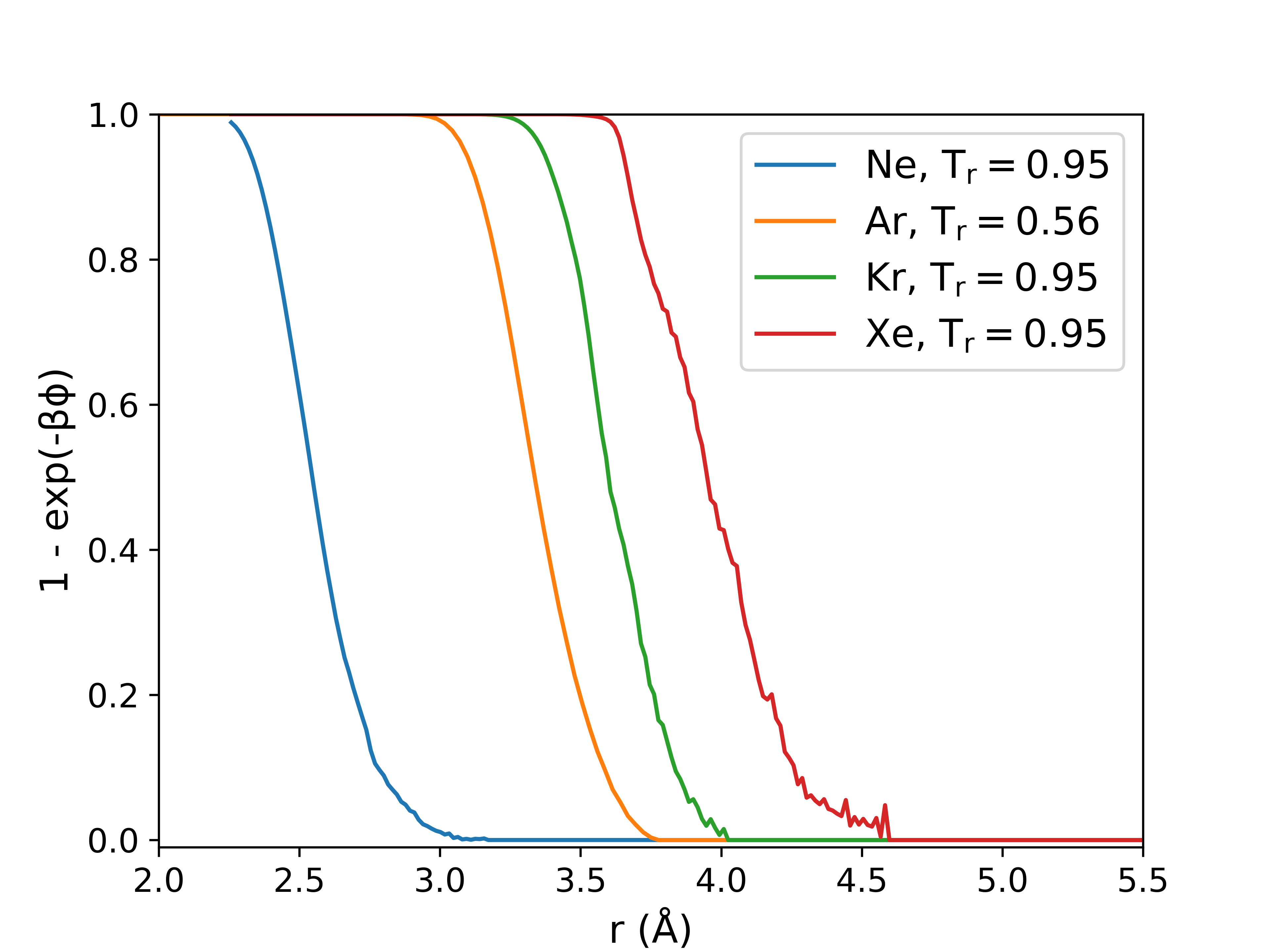
Figure 35: $[1-\exp(-\beta v_{0}(r))]$ for WCA separated SOPR potentials.

Figure 36 shows the hard-particle diameter calculated from (54) versus the electron polarizability along with results compiled from Fedordov et. al. and collision diameter estimates from quantum pair potentials. It is immediately striking that the classical prediction exhibits significantly different behavior than the other three methods. Furthermore, we can see that the two methods of estimating the atom size with quantum mechanical methods, i.e. the quantum Drude oscillator approximation in red and advanced electron structure calculations in black, give the same scaling behavior estimated from the neutron data. This result is exciting since it provides experimental validation for the quantum mechanics calculations and demonstrates that SOPR potentials can provide estimates of fundamental atomic properties consistent with quantum theory despite the method being semi-classical.

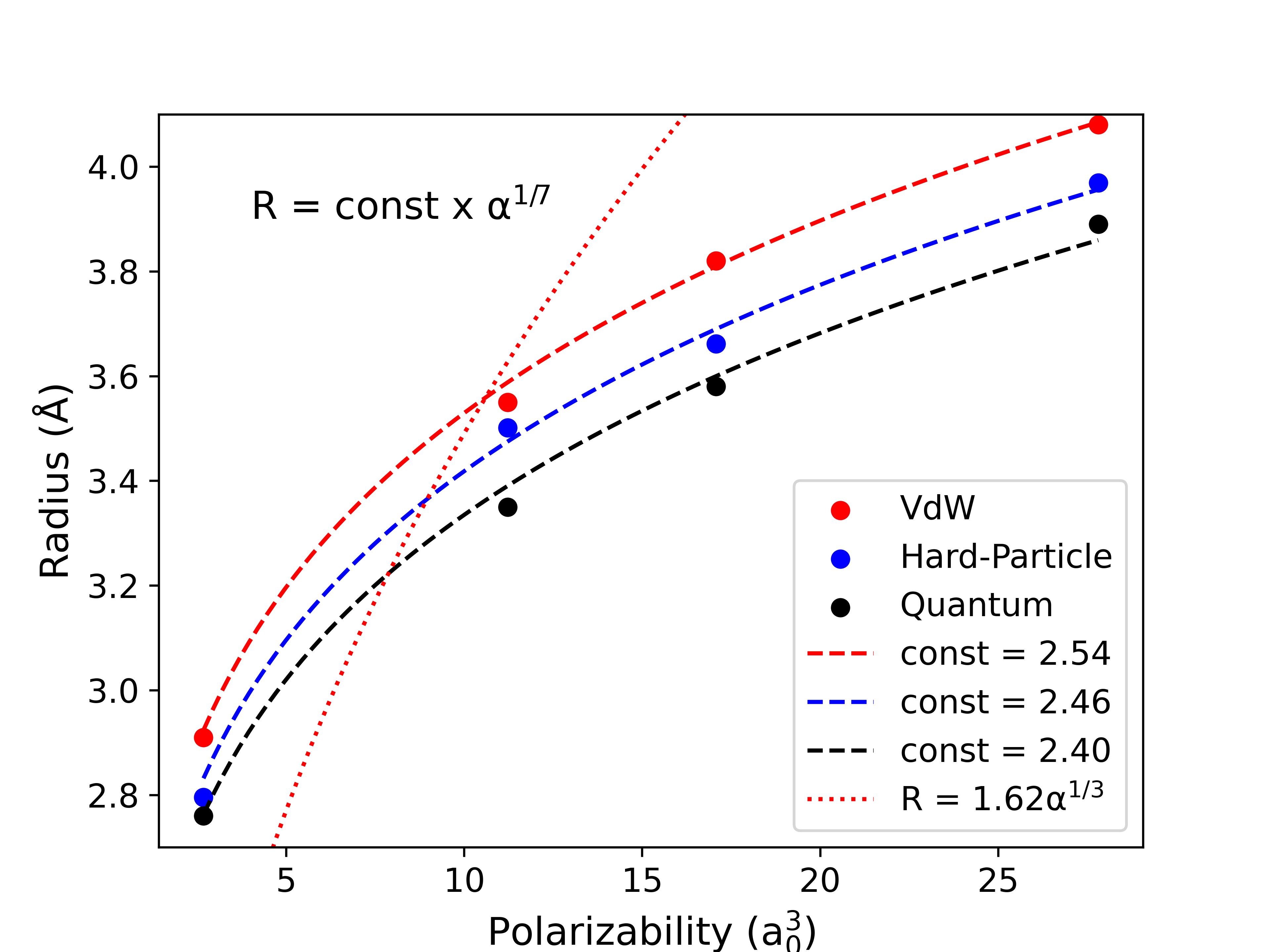
Figure 36: Particle radius determined from the van der Waal radius criterion (red dashed line and points), hard-particle radius derived from SOPR potentials (blue dashed line and points), and the quantum dimer potentials (black dashed line and points).

A.2 State-Dependent Corrections in Supercritical Krypton

Supercritical fluids have been the subject of intense investigation in recent years, owing largely to their applications as chemical solvents in industrial processes and recurrence in the physics of extreme environments [230]. At subcritical temperatures, violations of classical thermodynamic stability criterion characterize phase transitions. Specifically, vapor-liquid phase separation initiated via nucleation occurs at thermodynamic paths of constant chemical potential (binodal) while spontaneous vapor-liquid separation occurs when the curvature of the free energy with respect to composition becomes negative (spinodal). The critical point is defined as the extremum of the spinodal, beyond which there is no observable thermodynamic vapor-liquid phase separation. However, the fact that material properties of supercritical fluids are highly sensitive to changes in thermodynamic state (pressure, temperature, density, etc.) and have been shown to exhibit sharp inflections in such properties has motivated the search for a universal theory of fluids extending beyond the critical point [231, 232, 233, 234, 235]. Transitions in supercritical fluids have been proposed based on the behavior of thermodynamic and dynamical properties, including thermal conductivity, density fluctuations [236], density distribution functions [237, 238], velocity autocorrelation functions, specific heat, speed of sound, and diffusion.

One proposed theory of supercritical fluids asserts that inflections in the observed material properties can be attributed to the ability of the fluid to sustain significant transverse excitation modes [239, 240, 241]. Conceptually, this transition occurs at the Frenkel time scale $\tau_{F}$, defined as the average time required for the mean squared displacement of a particle to equal its effective particle size. This transition is referred to as the Frenkel line. While a precise theoretical framework for defining the Frenkel line has not been clearly identified, simulation and experimental evidence of inflections in model and real fluid properties near the Frenkel line have been observed. Of considerable interest is a recent neutron scattering study on supercritical krypton that reported the emergence of medium range order ($\sim$ 7-10Å) in the radial distribution function at $\sim$ 110 MPa along the 310K isotherm, indicating a transition from non-rigid to rigid dynamics that was attributed to crossing the Frenkel line [36]. The authors noted that empirical potentials derived from the neutron scattering analysis technique empirical potential structure refinement (EPSR) significantly deviated from a standard (12-6) Lennard-Jones potential, a model potential that is often used to approximate the Frenkel line with molecular simulation techniques. However, EPSR potentials are known to be unreliable in the prediction of thermodynamic properties as the technique was designed to determine molecular configurations consistent with experimental scattering rather than estimate physically accurate or transferable potentials. Thus, systematic analysis of the state-dependence of the interatomic potentials for supercritical krypton remains unresolved.

In addition to the proposed Frenkel line transition, there has also been work investigating supercritical phase transitions based on a maximum in the local correlation length in the pressure-temperature diagram (the Widom line) [242, 243, 239, 244] as well as a change in the oscillatory behavior of the radial distribution function (the Fisher-Widom line) [245]. Here we will focus on supercritical transitions defined by the radial distribution function; namely, the Fisher-Widom and pair correlation definition of the Frenkel transition. Figures 37 and 38 show what neutron scattering data is available on the krypton phase diagram as well as a plot of radial distribution functions reported in the literature [104, 36].

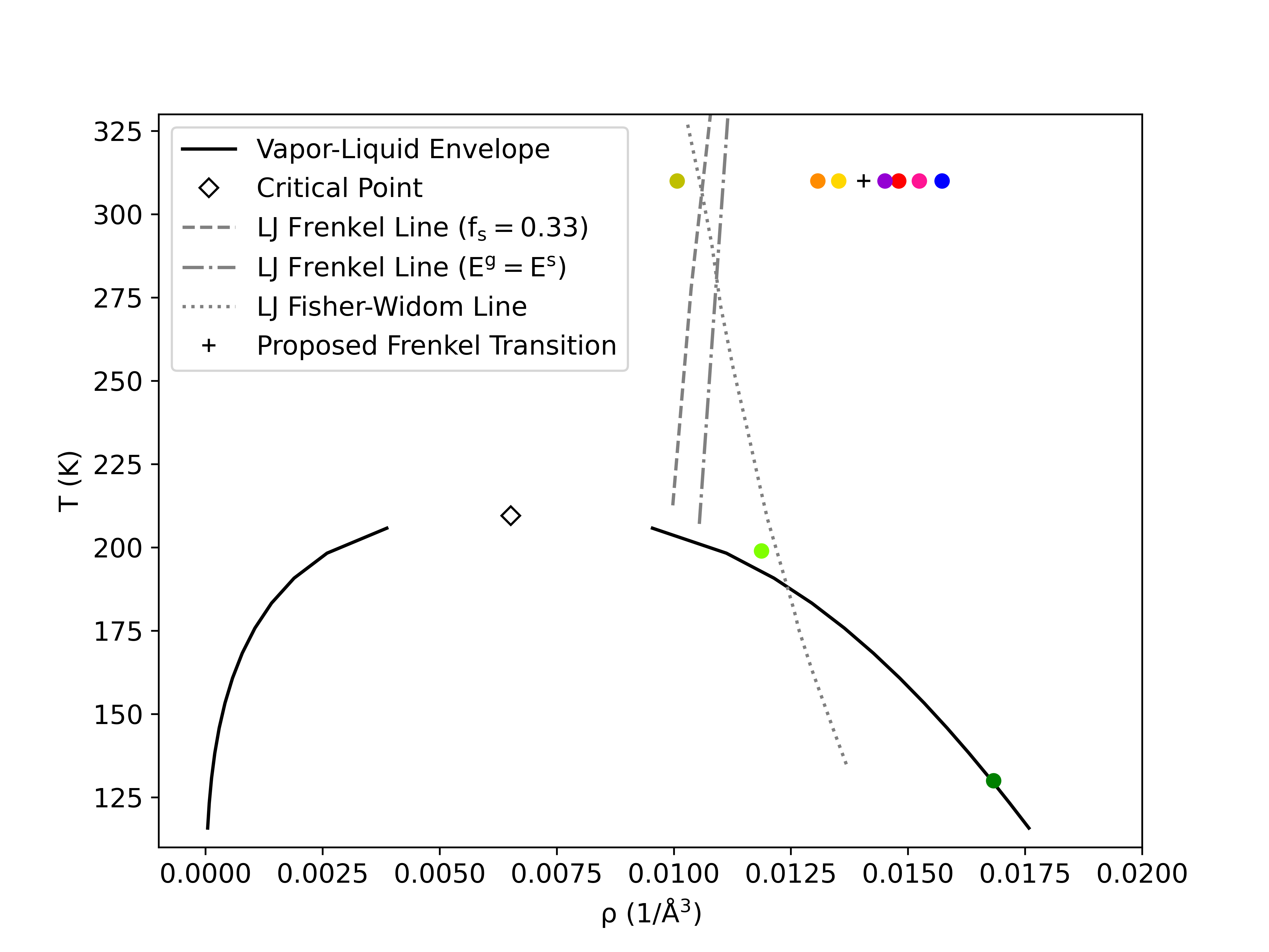
Figure 37: Phase diagram of krypton with neutron scattering experiments (colored points) and proposed supercritical transition lines drawn in based on results for the Lennard-Jones fluid.

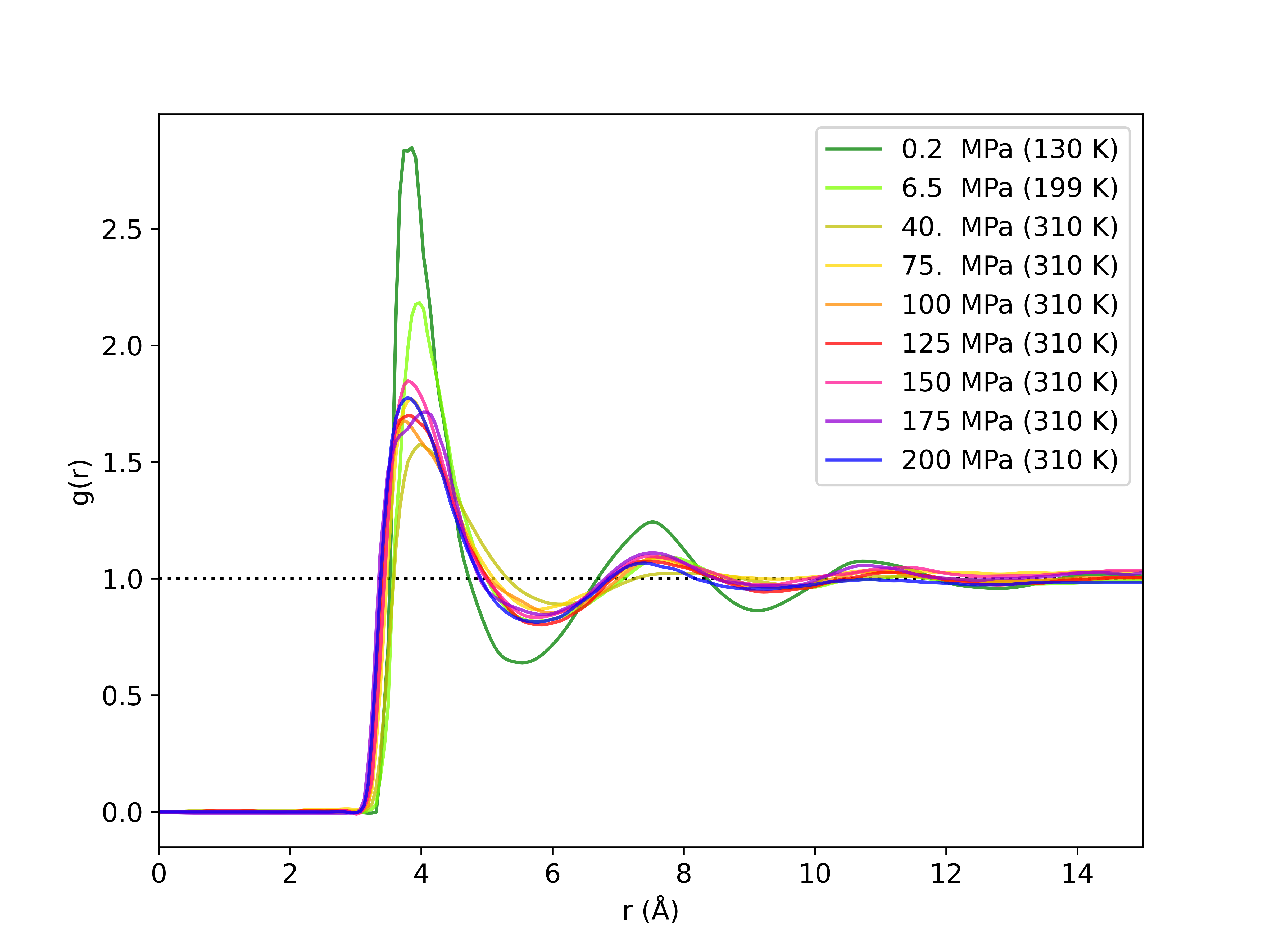
Figure 38: Available radial distribution functions derived from neutron scattering data for krypton.

Looking at Figure 37, we can see that there are two data points (camo green and neon green) that fall to the left of the Fisher-Widom transition, while the rest fall to the right. According to Fisher and Widom’s hypothesis, the oscillatory behavior of the radial distribution functions to the left of this transition should exhibit an always positive exponential decay whereas those to the right should be oscillatory [246]. Seeking the first experimental evidence for this transition, we computed the quantity $\log rh(r)$ from the neutron scattering derived radial distribution functions to see if this behavior is observed in Figure 39.

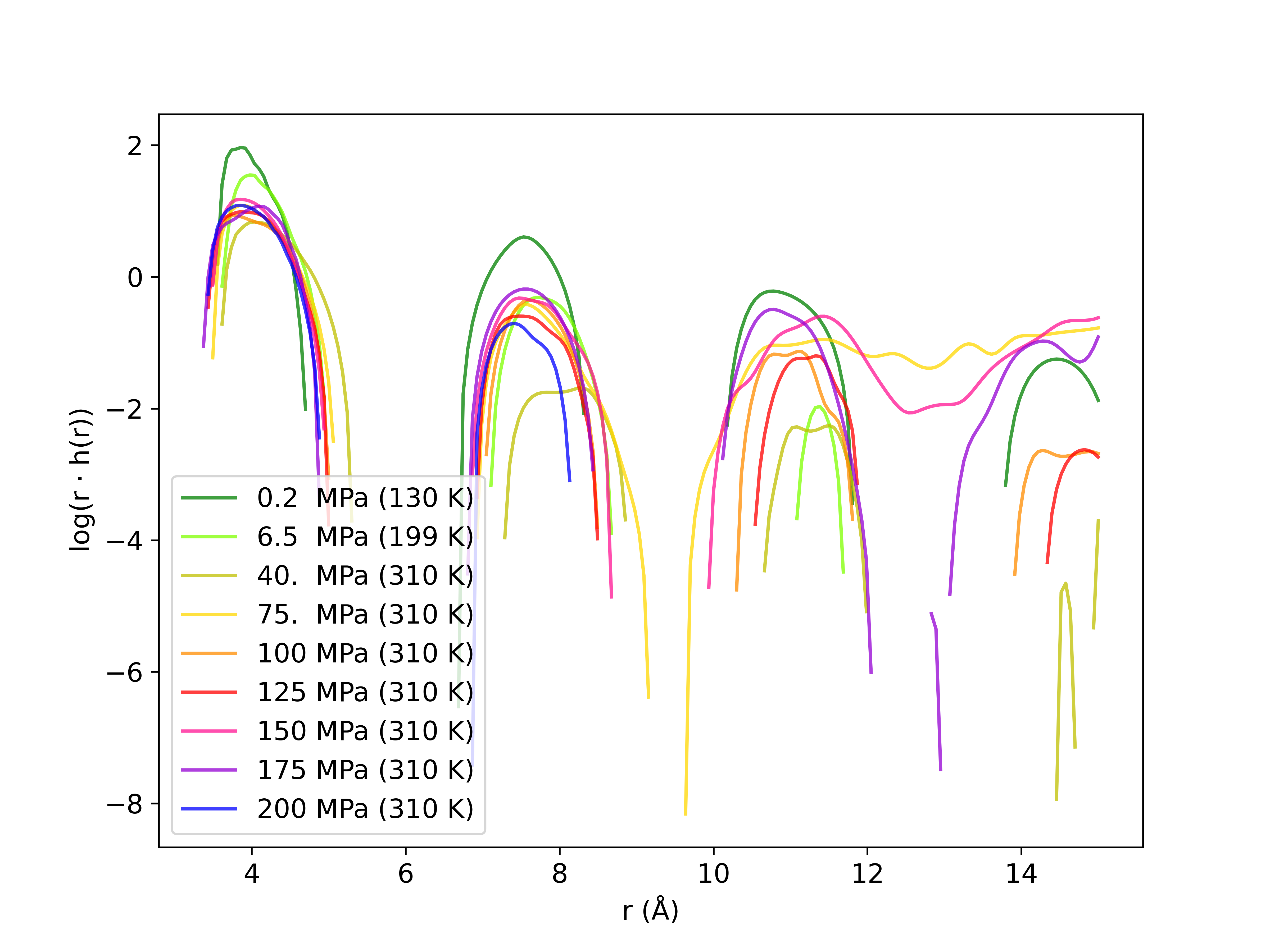
Figure 39: $\log rh(r)$ for available radial distribution function for krypton.

Monotonic decay at long range is not observed for the two conditions left of the Fisher-Widom line but is observed for two conditions right of the transition. Therefore, it is concluded that the neutron data available does not support a supercritical transition across the Fisher-Widom line for krypton. However, it is notable that the neutron scattering measurements used to derive these radial distribution functions may not be accurate enough to observe this subtle effect. For instance, all of the krypton scattering measurements reported had random errors larger than those identified in Chapter 4 for structural inversion analysis and the 2022 dataset of high pressure supercritical appears to show systematic errors in the raw scattering data (see Supporting Information from Pruteanu et. al [36]).

The next steps of this work are to apply structure-optimized potential refinement to quantify state-dependent many-body contributions to structure derived effective pair potentials. SOPR has been shown to predict transferable potentials in the subcritical region, challenging the established notion that state-dependent structure derived potentials are non-transferable to macroscopic thermodynamic property predictions. If the SOPR potentials do not significantly change along the 310 K isotherm and show no discernible change when crossing the Frenkel line, then we can conclude that there is no evidence of a transition in the interatomic forces across the proposed transition. Otherwise, we would be able to provide evidence of a transition in the interatomic forces that is independent of a thermodynamic phase transition.

Appendix B Statistical Mechanics of Liquid Phase Systems

The following appendix comprises the key results used in my lectures on statistical mechanics and molecular simulations during the Fall, 2023 term at the University of Utah. The mathematical framework presented here forms the foundation of the statistical mechanical results presented in this thesis. The main references used in compiling these lectures were the following:

1. Statistical Mechanics for Engineers - Isamu Kusaka [247]

2. Thermodynamics - Herbert Callen [248]

3. Thermodynamics - Enrico Fermi [249]

4. The Collected Works of J. Willard Gibbs [250]

5. Theory of Simple Liquids - Hansen and McDonald [17]

B.1 Classical Thermodynamics

An agglomerate of matter consists of an enormous amount of atoms. A single glass of water contains somewhere between $10^{24}$ and $10^{25}$ atoms alone! From a classical mechanics point of view, modeling the glass of water would require solving momentum equations for all $10^{25}$ atoms simultaneously. Clearly, this is beyond even the most powerful supercomputers that exist today. So, the question becomes, how can we study systems composed of an inconceivable number of particles without appealing to classical mechanics?

The characteristic time period of an atomic motion is on the order of $10^{-15}$ seconds. Therefore, even during a measurement of a system that is captured in a single microsecond, the atoms of a typical solid still go through ten million vibrations. This implies that a macroscopic measurement senses only averages of the atomic coordinates.

A map of how the atomic coordinates change is known as a normal mode. A normal mode is a coupled motion of atomic coordinates that include divergence (increase in particle density), convergence (decrease in particle density), and vibration. Some normal modes can be seen macroscopically, such as a change in volume or electric dipole. Others, like atomic vibrations, cannot be seen and are therefore "lost" in macroscopic observation. Classical thermodynamics is concerned with normal modes that are observable on a macroscopic scale.

By taking this macroscopic view, we lose a sense of how the motions of atomic coordinates can transfer energy. In Thermodynamics, we refer to this "invisible" mode of energy transfer as heat. From the Classical Mechanics perspective, heat is non-existent, since the energy of the system is completely characterized by generalized momentum and position for each particle. From this perspective, conservation of energy of a closed system requires that the change in energy be directly equal to the classical mechanical work done on the system, W’

$$\Delta E=W^{\prime}.$$ (55)

To accommodate the fact that we cannot observe all forms of energy transfer macroscopically (what we will call work), we must split the W’ into observable energy transfer, W, and unobservable energy transfer, Q (heat). This gives us the first law of thermodynamics

$$\Delta E=W+Q.$$ (56)

Now, in thermodynamics we are not typically concerned with the motion of a system in space or its change in position with respect to an external field, so we can simplify our energy conservation equation to simply include the internal energy, U,

$$\Delta U=W+Q$$ (57)

where W and Q are path functions, meaning that they depend on the exact way that changes are brought about by them. W is a path function because, in defining it, we have lost track of microscopic displacements, whereas classical mechanical work W’ is a path-independent function. An infinitesimal view of this equation is shown below,

$$dU={\mathchar 22\relax\mkern-12.0mud}W+{\mathchar 22\relax\mkern-12.0mud}Q$$ (58)

where $\;{\mathchar 22\relax\mkern-12.0mud}$ indicates an imperfect differential. The differential is imperfect since W and Q are path-dependent functions.

B.1.1 Thermodynamic Postulates

Thermodynamics is concerned with both reversible and irreversible processes, but for now let us consider equilibrium thermodynamics. An equilibrium state is a state of the system that, given a certain set of internal parameters U, V, and $N_{i}$ (i = 1, …, n), the system tends to evolve towards. This leads us to the first postulate.

Postulate B.1.

There exist particular states, called equilibrium states, that are completely characterized by U, V, $N_{i}$ (i = 1, …, n).

Note that in more complex systems, we require an inclusion of elastic strain parameters and electric dipole moment (also macroscopically measurable properties). A system at macroscopic equilibrium is a system where all representative atomic states of the system exist in the time scale of a macroscopic measurement.

Postulate B.2.

There exists a function, S, such that, S = S(U,V,N). Furthermore, the extensive parameters take values so that this function is maximized over the manifold of constrained equilibrium states.

This postulate applies only to equilibrium states, but in general not to non-equilibrium states. Essentially, we are postulating the existence of some function, called the entropy, that is maximized at equilibrium with respect to all of its dependent variables. The following two postulates apply to properties of the entropy and they are shown below.

Postulate B.3.

Entropy is additive over subsequent subsystems. Furthermore, S is a continuous, differentiable, and a monotonically increasing function of energy.

There are immediate consequences of this postulate which are listed below.

Corollary B.3.1.

$$S=\sum_{\alpha}S^{(\alpha)}$$ (59)

Corollary B.3.2.

The entropy of a simple system is a homogeneous, first-order function of the extensive parameters.

$$S(\lambda U,\lambda V,\lambda N)=\lambda S(U,V,N)$$ (60)

Corollary B.3.3.

The monotonic property implies that temperature is non-negative. In other words,

$$\left(\frac{\partial S}{\partial U}\right)_{V,N}>0.$$ (61)

Corollary B.3.4.

Entropy can be inverted with respect to energy because it is a single-valued, continuous, and differentiable function with respect to S, V, N.

Postulate B.4.

The entropy of any system vanishes in the state when T = 0.

B.2 The 2nd Law of the Thermodynamics

Entropy can change as a result of internal or external processes. We express the differential change in entropy as,

$$dS={\mathchar 22\relax\mkern-12.0mud}{S_{e}}+{\mathchar 22\relax\mkern-12.0mud}{S_{i}}.$$ (62)

We now accept that the expression for ${\mathchar 22\relax\mkern-12.0mud}{S_{e}}$ is given by,

$${\mathchar 22\relax\mkern-12.0mud}{S_{e}}=\frac{{\mathchar 22\relax\mkern-12.0mud}{Q}}{T}.$$ (63)

On the other hand, an important consequence of of the second law is that,

$${\mathchar 22\relax\mkern-12.0mud}{S_{i}}\geq 0.$$ (64)

Equality holds in the previous equation when the process is reversible. A reversible process is such that the sequence of states visited by the system can be traversed in the opposite direction by an infinitesimal change in the boundary conditions. According to the second law, processes resulting in a decrease of the entropy are impossible for an isolated system. In terms of statistical mechanics, this is not actually the case (as will be seen later).

B.2.1 Violating the 2nd Law: Maxwell’s Demon

Maxwell’s demon is a thought experiment which shows how the second law can be violated. In Maxwell’s words, "… if we conceive of a being whose faculties are so sharpened that he can follow every molecule in its course, such a being, whose attributes are as essentially finite as our own, would be able to do what is impossible to us. For we have seen that molecules in a vessel full of air at uniform temperature are moving with velocities by no means uniform, though the mean velocity of any great number of them, arbitrarily selected, is almost exactly uniform. Now let us suppose that such a vessel is divided into two portions, A and B, by a division in which there is a small hole, and that a being, who can see the individual molecules, opens and closes this hole, so as to allow only the swifter molecules to pass from A to B, and only the slower molecules to pass from B to A. He will thus, without expenditure of work, raise the temperature of B and lower that of A, in contradiction to the second law of thermodynamics."

B.2.2 The Fundamental Relation

To this point we have discussed entropy as a function on internal energy, volume, and the number of moles of each chemical species. We know that based on the properties of this function that we can solve for internal energy directly and it will be a function of entropy, volume, and the number of moles of each chemical species. Thus,

$$U=\left[U(S,V,N_{i}):i=(1,...,n)\right].$$ (65)

To examine infinitesimal changes in the energy, we compute the first differential of U to obtain,

$$dU=\left(\frac{\partial U}{\partial S}\right)_{V,N}dS+\left(\frac{\partial U}{\partial V}\right)_{S,N}dV+\sum_{i}\left(\frac{\partial U}{\partial N_{i}}\right)_{S,V}dN_{i}.$$ (66)

The previous partial derivatives are called intensive parameters, and are given the following definitions.

$$\left(\frac{\partial U}{\partial S}\right)_{V,N}\equiv T$$ (67)

$$\left(\frac{\partial U}{\partial V}\right)_{S,N}\equiv-P$$ (68)

$$\left(\frac{\partial U}{\partial N_{i}}\right)_{S,V}\equiv\mu_{i}.$$ (69)

With these definitions, the first differential dU can be expressed as,

$$dU=TdS-PdV+\sum_{i}\mu_{i}dN_{i}.$$ (70)

It should now be clear that ${\mathchar 22\relax\mkern-12.0mud}{Q}=TdS$, ${\mathchar 22\relax\mkern-12.0mud}{W_{m}}=-PdV$ (as shown previously), and that we have an additional work term known as the quasi-static chemical work, ${\mathchar 22\relax\mkern-12.0mud}{W_{c}}=\sum_{i}\mu_{i}dN_{i}$. We should note, however, that this does not hold for irreversible processes since these are path-dependent functions.

B.2.3 Equations of State

The intensive parameters defined previously are functions of S,V,N since they are partial derivatives of a function of those variables. Therefore,

$$T=T(S,V,N_{i})$$ (71)

$$P=P(S,V,N_{i})$$ (72)

$$\mu_{i}=\mu_{i}(S,V,N_{i}).$$ (73)

These relationships that express intensive parameters in terms of the extensive parameters, are known as equations of state. In addition, since the fundamental relation is homogeneous first order, equations of state are homogeneous zero order. In other words,

$$T(\lambda S,\lambda V,\lambda N_{i})=T(S,V,N_{i}).$$ (74)

Physically, we can interpret this as the temperature of two subsystems of a composite system is not additive. In fact, at equilibrium, any number of subsystems chosen from a composite system will have the same temperature as the composite system as a whole.

B.2.4 The Euler Form

Recall the first order homogeneous property of the fundamental relation.

$$U(\lambda S,\lambda V,\lambda N)=\lambda U(S,V,N).$$ (75)

Differentiating with respect to $\lambda$, we find,

$$U=\left(\frac{\partial U}{\partial(\lambda S)}\right)_{V,N}\frac{\partial(\lambda S)}{\partial\lambda}+\left(\frac{\partial U}{\partial(\lambda V)}\right)_{S,N}\frac{\partial(\lambda V)}{\partial\lambda}+\sum_{i}\left(\frac{\partial U}{\partial(\lambda N_{i})}\right)_{S,V}\frac{\partial(\lambda N_{i})}{\partial\lambda}.$$ (76)

This is true for any value of $\lambda$. Simplifying this expression and taking $\lambda=1$,

$$U=TS-PV+\sum_{i}\mu_{i}N_{i}.$$ (77)

B.2.5 The Gibbs-Duhem Relation

Taking the Euler form of the fundamental relation and taking an infinitesimal variation gives,

$$dU=TdS+SdT-PdV-VdP+\sum_{i}\mu_{i}dN_{i}+\sum_{i}N_{i}d\mu_{i}.$$ (78)

However, we know that the proper form of the equation from the fundamental relation is,

$$dU=TdS-PdV+\sum_{i}\mu_{i}dN_{i}.$$ (79)

We then take the difference between these two relations to obtain the Gibbs-Duhem Relation,

$$0=SdT-VdP+\sum_{i}N_{i}d\mu_{i}.$$ (80)

This relation demonstrates the intensive parameters (T, P, and $\mu$), cannot be varied independently. In addition, this relation shows that in a system of n components, n + 1 intensive parameters can be varied independently. This is referred to as the thermodynamic degrees of freedom of the system.

B.2.6 Gibbs Phase Rule

The interface between coexisting phases may be regarded as a partition that is diathermal, movable, and permeable to all species. Thus, at equilibrium, there must be a consistency in temperature, pressure, and chemical potential across all M phases.

$$T_{1}=T_{2}=...=T_{M}$$ (81)

$$P_{1}=P_{2}=...=P_{M}$$ (82)

$$\mu_{1}=\mu_{2}=...=\mu_{M}.$$ (83)

If we perturb the state of the system by increasing the temperature by some $dT$, then in order to preserve the M phases, each phase parameter must be preserved after this change as well.

$$T_{1}+dT_{1}=T_{2}+dT_{2}=...=T_{M}+dT_{M}$$ (84)

$$P_{1}+dP_{1}=P_{2}+dP_{2}=...=P_{M}+dP_{M}$$ (85)

$$\mu_{1}+d\mu_{1}=\mu_{2}+d\mu_{2}=...=\mu_{M}+d\mu_{M}.$$ (86)

Thus we find that,

$$dT_{1}=dT_{2}=...=dT_{M}$$ (87)

$$dP_{1}=dP_{2}=...=dP_{M}$$ (88)

$$d\mu_{1}=d\mu_{2}=...=d\mu_{M}.$$ (89)

Now, these relationships must be consistent with the Gibbs-Duhem relation, namely,

$$0=SdT-VdP+\sum_{i}^{n}N_{i}d\mu_{i}.$$ (90)

If we hold pressure constant and vary only temperature, we find that,

$$0=S^{(j)}dT+\sum_{i}^{n}N^{(j)}_{i}d\mu_{i}$$ (91)

for all phases $1,...,M$. But this requires that $dT$ and $d\mu_{i}$ are zero. That is, if we want to perturb the state of the system while maintaining the phase coexistence, we cannot possibly hold P constant. We now have (n + 2) infinitesimal quantities with M equations. Therefore, to ensure the system has solutions, we can only specify (n + 2 - M) of those variables independently. This is known as the Gibbs phase rule.

B.2.7 Free Energies and the General Legendre Transform

The Legendre transform is a mathematical tool that allows us to replace the extensive parameters as independent variables with intensive parameters. In general, the fundamental relation may be expressed as,

$$Y=Y(X_{0},X_{1},...X_{t}).$$ (92)

This gives a hyper-surface in a (t+2)-dimensional space with Cartesian coordinates $Y,X_{0},X_{1},...X_{t}$. The partial slope of this hyper-surface is given by,

$$P_{k}=\frac{\partial Y}{\partial X_{k}}.$$ (93)

Now, the hyper-surface may be defined by the fundamental relation, or by the envelope of the tangent hyper-planes. If we consider the intercept of the hyper-plane, $\psi$, as a function of the slopes, then we obtain a relation,

$$P_{k}=\frac{Y-\psi}{X_{k}-0}.$$ (94)

This is simply the "rise over run" equation for the slope. Now, this means that for any k,

$$Y-P_{k}X_{k}=\psi.$$ (95)

Performing this calculation for all (t+1) dimensions gives the relation,

$$Y-\sum_{0}^{t+1}P_{k}X_{k}=\psi.$$ (96)

Thus, taking the partial derivative with respect to $P_{k}$ gives,

$$-X_{k}=\frac{\partial\psi}{\partial P_{k}}.$$ (97)

Legendre transformed fundamental relations are called thermodynamic potentials.

B.2.8 The Helmholtz Potential

Suppose that we take the fundamental relation in the energy representation, $U=U(S,V,N_{i})$. Then the slope of the hyper-surface formed by this fundamental relation has the usual form,

$$P_{k}=\frac{\partial U}{\partial X_{k}}.$$ (98)

Specifically, if we consider the entropy as an extensive variable we would like to remove, we consider,

$$T=\frac{\partial U}{\partial S}.$$ (99)

Then, we consider the intercepts of the tangent hyper-surface of this variable; namely,

$$T=\frac{U-F}{S-0}.$$ (100)

where $F$ is the name of the function of intercepts with zero entropy. Rearranging this equation we find the Helmholtz potential,

$$F=U-TS.$$ (101)

Now, we have found $F=F(T,V,N_{i})$. Thus, we can compute the first differential to determine,

$$dF=\left(\frac{\partial F}{\partial T}\right)_{V,N}dT+\left(\frac{\partial F}{\partial V}\right)_{T,N}dV+\sum_{i}\left(\frac{\partial F}{\partial N_{i}}\right)_{T,V}dN_{i}.$$ (102)

But, from the relation $F=U-TS$, taking the first differential gives,

$$dF=dU-TdS-SdT.$$ (103)

Recall that the internal energy is given by,

$$dU=TdS-PdV+\sum_{i}\mu_{i}dN_{i}.$$ (104)

so we substitute this expression in and find,

$$dF=-SdT-PdV+\sum_{i}\mu_{i}dN_{i}.$$ (105)

This indicates the definitions of the partial derivatives of the Helmholtz potential.

$$\left(\frac{\partial F}{\partial T}\right)_{V,N}=-S$$ (106)

$$\left(\frac{\partial F}{\partial V}\right)_{T,N}=-P$$ (107)

$$\sum_{i}\left(\frac{\partial F}{\partial N_{i}}\right)_{T,V}=\mu_{i}.$$ (108)

The enthalpy is found by taking the legendre transform of U by replacing V with P, and the Gibbs potential is found by replacing S and V with T and P.

B.2.9 The Maxwell Relations

The Maxwell relations are simply a statement of the equality of the mixed partial derivatives of the fundamental relation.

$$\frac{\partial^{2}U}{\partial S\partial V}=\frac{\partial^{2}U}{\partial V\partial S}$$ (109)

$$-\left(\frac{\partial P}{\partial S}\right)_{V,N_{i}}=\left(\frac{\partial T}{\partial V}\right)_{S,N_{i}}.$$ (110)

Given a thermodynamic potential with $(t+1)$ natural variables, there are $\frac{t(t+1)}{2}$ separate pairs of mixed partial derivatives and thus that many Maxwell relations.

B.2.10 Jacobian Transformations

An excellent method for manipulation of thermodynamic derivatives is based on the mathematical properties of Jacobians. If $u,v....w$ are functions of $x,y,...z$, the Jacobian is defined as,

$$\frac{\partial(u,v,...,w)}{\partial(x,y,...,z)}\equiv\begin{vmatrix}\frac{\partial u}{\partial x}&\frac{\partial u}{\partial y}&...&\frac{\partial u}{\partial z}\\ \frac{\partial v}{\partial x}&\frac{\partial v}{\partial y}&...&...\\ \frac{\partial w}{\partial x}&...&...&\frac{\partial w}{\partial z}\end{vmatrix}.$$ (111)

The property that makes this incredibly useful in thermodynamics is the relationship,

$$\left(\frac{\partial u}{\partial x}\right)_{y...z}=\frac{\partial(u,y,...,z)}{\partial(x,y,...,z)}$$ (112)

Jacobians have the following nice properties.

$$\frac{\partial(u,v,...,w)}{\partial(x,y,...,z)}=-\frac{\partial(v,u,...,w)}{\partial(x,y,...,z)}$$ (113)

$$\frac{\partial(u,v,...,w)}{\partial(x,y,...,z)}=\frac{\partial(u,v,...,w)}{\partial(r,s,...,t)}\frac{\partial(r,s,...,t)}{\partial(x,y,...,z)}$$ (114)

$$\frac{\partial(u,v,...,w)}{\partial(x,y,...,z)}=1/\frac{\partial(x,y,...,z)}{\partial(u,v,...,w)}.$$ (115)

B.2.11 The Nernst Postulate

The third law of thermodynamics, otherwise known as the Nernst postulate, states that,

Postulate B.5.

The entropy of a system approaches a constant value at absolute zero temperature.

From a microstate perspective, at absolute zero temperature there is either only one unique microstate, known as the ground state, or there are a set of minimum energy microstates, which are finite. An equivalent statement of the nernst postulate is,

Postulate B.6.

It is impossible by any procedure, no matter how idealized, to reduce the temperature of any closed system to zero temperature in a finite number of finite operations.

Suppose that the temperature of a substance can be reduced in an isentropic process by changing the parameter X from X2 to X1. One can think of a multistage nuclear demagnetization setup where a magnetic field is switched on and off in a controlled way. If there were an entropy difference at absolute zero, T = 0 could be reached in a finite number of steps. However, at T = 0 there is no entropy difference so an infinite number of steps would be needed.

B.2.12 Stability of Thermodynamic Systems

The requirement that the second derivative of energy be positive gives rise to some interesting findings. To see this, let’s first construct an intrinsic system and a complimentary subsystem from a composite, isolated system. The complimentary subsystem is assumed to be much larger than the intrinsic subsystem. The fundamental relation is given by,

$$U^{\prime}=X_{t}u(x_{0},x_{1},...,x_{t-1}+\tilde{X}_{t}\tilde{u}(\tilde{x}_{0},\tilde{x}_{1},...,\tilde{x}_{t-1})$$ (116)

where $X_{t}$ represents some parameter of the fundamental relation that is being held constant. Furthermore, the smallness of the intrinsic system compared to the complementary system requires that,

$$|d\tilde{x}_{i}|<<|dx_{i}|.$$ (117)

Now, any changes in the $x_{i}$ leads to a total change in energy. We can express the energy change in terms of a Taylor expansion such that,

$$\Delta U^{\prime}=X_{t}[du+d^{2}u+...]+\tilde{X}_{t}d\tilde{u}$$ (118)

where,

$$du=\sum_{i}\frac{\partial u}{\partial x_{i}}dx_{i}$$ (119)

$$d^{2}u=\frac{1}{2!}\sum_{j}\sum_{i}\frac{\partial^{2}u}{\partial x_{i}\partial x_{j}}dx_{i}dx_{j}.$$ (120)

We can neglect higher order terms of $\tilde{u}$ since we are assuming that the changes in the independent variables are very small for the complimentary system. Now, since the composite system is isolated, by our usual formalism the change in internal energy for the composite system vanishes,

$$0=X_{t}\sum_{i}\frac{\partial u}{\partial x_{i}}dx_{i}+\tilde{X}_{t}\sum_{i}\frac{\partial\tilde{u}}{\partial\tilde{x}_{i}}d\tilde{x}_{i}.$$ (121)

This leads us to the usual results that all of the intensive parameters (T, P, $\mu_{i}$) are the same in each subsystem at equilibrium. In other words, the composite system is homogeneous. However, we now turn our attention to the second requirement; namely,

$$d^{2}u=\frac{1}{2!}\left[\sum_{0}^{t-1}\sum_{0}^{t-1}\frac{\partial^{2}u}{\partial x_{i}\partial x_{j}}dx_{i}dx_{j}\right]>0.$$ (122)

The quantity in brackets is known as the homogeneous quadratic form. The condition that the quadratic form be positive for all combinations of variables is referred to mathematically as the condition that the quadratic form be positive definite.

Notice that we have numerous cross terms in the expression for $d^{2}u$. The presence of these cross terms make it difficult to determine what quantities must be positive, so we need to perform a linear transformation such that the quadratic form is a sum of squares. Sylvester’s law of inertia guarantees that no matter which transformation we pick, the number of positive, negative, and zero coefficients will be the same.

For this discussion, we will proceed by considering terms that contain $dx_{0}$. We can thus express the equation as,

$$d^{2}u=\frac{1}{2}\left[u_{00}^{2}(dx_{0})^{2}++2\sum_{1}^{t-1}\frac{\partial^{2}u}{\partial x_{0}\partial x_{k}}dx_{0}dx_{k}+\sum_{1}^{t-1}\sum_{1}^{t-1}\frac{\partial^{2}u}{\partial x_{i}\partial x_{j}}dx_{i}dx_{j}\right]>0.$$ (123)

We now eliminate the cross terms by introducing the new variable, $dP_{0}$.

$$dP_{0}=u_{00}dx_{0}+\sum_{1}^{t-1}u_{0k}dx_{k}$$ (124)

$$(dP_{0})^{2}=u_{00}^{2}(dx_{0})^{2}+2u_{00}\sum_{1}^{t-1}u_{0k}dx_{k}+\sum_{1}^{t-1}\sum_{1}^{t-1}u_{0j}u_{0k}dx_{j}dx_{k}$$ (125)

which allows us to express the second derivative of internal energy as,

$$d^{2}u=\frac{1}{2}\left[\frac{1}{u_{00}}(dP_{0})^{2}+\sum_{1}^{t-1}\sum_{1}^{t-1}(u_{jk}-\frac{u_{0j}u_{0k}}{u_{00}})dx_{j}dx_{k}\right]>0.$$ (126)

Now, notice that the previous equation can be rewritten as,

$$d^{2}u=\frac{1}{2}\left[\frac{1}{u_{00}}(dP_{0})^{2}+\sum_{1}^{t-1}\sum_{1}^{t-1}(u_{jk})_{P_{0},x_{1},x_{2},...}dx_{j}dx_{k}\right]>0.$$ (127)

We can rewrite this expression in a helpful way. Consider the following mathematical fact,

$$\bigg{(}u_{jk}-\frac{u_{0j}u_{0k}}{u_{00}}\bigg{)}=\bigg{(}\frac{\partial^{2}(u-P_{0}x_{0})}{\partial x_{j}\partial x_{k}}\bigg{)}_{P_{0},x_{1},...}=\frac{\partial^{2}\psi^{(0)}}{\partial x_{j}\partial x_{k}}.$$ (128)

The function $\psi^{(0)}$ is the Legendre transform of u with respect to $P_{0}$. This allows us to now write the second derivative of u as,

$$d^{2}u=\frac{1}{2}\left[\frac{1}{u_{00}}(dP_{0})^{2}+\sum_{1}^{t-1}\sum_{1}^{t-1}\psi_{jk}^{(0)}dx_{j}dx_{k}\right]>0.$$ (129)

Proceeding in this way, for each of the $dx_{i}$, we arrive at a useful form given by,

$$d^{2}u=\frac{1}{2}\sum_{0}^{t-1}\frac{1}{\psi_{jj}^{(j-1)}}(dP_{j}^{(j-1)})^{2}>0.$$ (130)

Thus, we require that all of the $\psi_{jj}^{(j-1)}$ be positive such that,

$$\psi_{jj}^{(j-1)}=\bigg{(}\frac{\partial P_{j}}{\partial x_{j}}\bigg{)}_{P_{0},P_{1}...P_{j-1},x_{j+1},x_{j+2}...x_{t-1}}>0.$$ (131)

So, what exactly does this mean? Common terms that must be positive according to this definition are,

$$-\bigg{(}\frac{\partial P}{\partial V}\bigg{)}_{T}>0$$ (132)

$$\bigg{(}\frac{\partial U}{\partial T}\bigg{)}_{v}=C_{v}>0.$$ (133)

Of course, depending on the complexity of the system, we can have many more relations from this procedure. However, in fluid phase transitions, we are typically most concerned with the first of the two explicit equations and the second is just assumed to be true.

B.3 Statistical Mechanics

B.3.1 Dynamical Variable Measurement

We have studied how particle positions and momenta evolve in time according to Hamilton’s equations of motion. Of course, when dealing with real systems, we are almost never concerned with the motion of all of the particles in the system and we know that materials can be well-described by simple thermodynamic laws. However, up to this point, you may feel a bit uneasy that we have swept the dynamics of particles under the rug when we discussed thermodynamics. So far, we collected all of the microscopic modes of energy transfer into the heat term and introduced the entropy fundamental relation. From these very simple assumptions we have found that we can derive nearly all of thermodynamics. But what is heat? Or entropy? To answer these questions, we need to study statistical mechanics. We will see that statistical mechanics is a powerful tool to unite microscopic dynamics with macroscopic theory. Statistical mechanics holds whether the system is classical or quantum mechanical, and has been applied to study systems as diverse as molecular systems, black holes, and bird flocking.

Recall that a dynamical variable was some variable $A=A(q^{f},p^{f},t)$. Let’s suppose that we want to measure the dynamic variable in the lab. How do we actually define what the true value is? Is it the value of $A$ at the specific instant in time we measure it? How do we accommodate for the fact that $A$ could be changing extremely fast due to atomic motions?

We can define the value of $A$ as its average over the amount of time that the variable is measured. If the time scale of the measurement is significantly larger than the time scale of molecular motion, the value of A that we measure will take the form,

$$A_{exp}=\lim_{\tau\rightarrow\infty}\frac{1}{\tau}\int_{t}^{t+\tau}A(q^{f}(t^{\prime}),p^{f}(t^{\prime}),t^{\prime})dt^{\prime}$$ (134)

which is just an integral relation for the time average of $A$ over a measurement time $\tau$. To see this, just consider that the integral is equivalent to adding up all of the contributions to $A$ over time and the $1/\tau$ term is dividing by the total time of the measurement. The limit ensures that the time measurement is long enough to accurately capture the average. This is analogous to taking an average of a set of measurements in which you add up all the measurement values and divide by the number of samples.

B.3.2 Phase Space

The mechanical state of a system is specified by 2f variables; namely, the momentum and generalized coordinates of the $f$ particles in a system. The mechanical state comprises some specific point in this space, and we refer to this point as the phase point. Over time, the phase point changes according to the equations of motion, and forms a phase trajectory.

B.3.3 Ensemble Average

Suppose that we allow some 1-D system to evolve over a time $\tau$. If we choose a volume element, then the probability that the system phase is in the volume element is given by,

$$\rho dq^{f}dp^{f}=\lim_{\tau\rightarrow\infty}\frac{\Delta t(q^{f},p^{f},t)}{\tau}$$ (135)

where $\Delta t$ is the total time that the particle spends in the volume element. We call $\rho=\rho(q^{f},p^{f},t)$ the probability density function. Now, we can combine the dynamical variable measurement for the volume element with our probability density definition to see that,

$$A_{exp}(t)=\int A(q^{f},p^{f},t)\rho(q^{f},p^{f},t)dq^{f}dp^{f}.$$ (136)

Note that this integration occurs over the entire phase space. Furthermore, note that this equation only holds if explicit time dependence of A occurs sufficiently slowly over $\tau$.

Since $\rho$ is a probability density function, it has a few special properties:

1. $\rho$ is a probability distribution function, so it must normalize to 1. This means that,

   $$\int\rho dq^{f}dp^{f}=1$$ (137)

2. $\rho$ must be non-negative so that, $\rho\leq 0$.

It is very reasonable to question why we would rewrite our original expression with some new, seemingly not useful function $\rho$. We haven’t really made too much progress computationally, as all we have done is rearranged the problem with some new definitions. However, the hope is that by defining $\rho$ in this way that we can find a $\rho$ to use in eq (136) that will allow us to solve for $A_{exp}(t)$ without ever needing to solve the equations of motion directly. Furthermore, by reformulating the motion of many-particles with respect to this probability density function, perhaps we can gain novel insight that would otherwise be difficult to describe or notice.

B.3.4 Statistical Equilibrium

Statistical equilibrium occurs when the change in all measured dynamic variables with respect to time is zero, unless the dynamic variable depends explicitly on time. This implies that at equilibrium $A=A(q^{f},p^{f})$, where the explicit time-dependence is dropped. Thus,

$$\frac{dA_{exp}}{dt}=\lim_{\Delta t\rightarrow 0}\frac{1}{\Delta t}\left[\int A(q^{f},p^{f})[\rho(q^{f},p^{f},t+\Delta t)-\rho(q^{f},p^{f},t)]\right]dq^{f}dp^{f}$$ (138)

and applying a first-order Taylor expansion on the probability density function gives,

$$\frac{dA_{exp}}{dt}=\lim_{\Delta t\rightarrow 0}\int A(q^{f},p^{f})\frac{\partial\rho}{\partial t}dq^{f}dp^{f}.$$ (139)

Therefore, the condition of statistical equilibrium is that $\rho$ does not depend explicitly on time, or,

$$\frac{\partial\rho}{\partial t}=0.$$ (140)

Since the previous expression must hold for any choice of $A$.

B.3.5 The Statistical Ensemble

The concept of a statistical ensemble was introduced by Gibbs. Let’s suppose that we make $\mathcal{N}$ identical copies of a system, and we completely transfer the explicit time dependence and Hamiltonian for each copy. This is known as the statistical ensemble. Now, the number of copies of the system that fall in the volume element $dq^{f}dp^{f}$ is given by,

$$\mathcal{N}\rho(q^{f},p^{f},t)dq^{f}dp^{f}.$$ (141)

This represents the number of copies in the phase space around the point $(q^{f},p^{f})$. Noting that copies of the system are neither generated nor destroyed in this process, the total copy density $N\rho$ is conserved.

B.3.6 Louiville’s Theorem and the Canonical Ensemble

Recall the equation of continuity from continuum mechanics. The equation of continuity amounts to writing down a mass balance on a system noting that the total mass of a system is conserved. For some fixed region of space, referred to as a control volume, the number of particles in the control volume at any moment $t$ is given by,

$$\int_{V}\rho(\mathbf{r},t)d\mathbf{r}$$ (142)

where $V$ denotes the control volume and $\rho(\mathbf{r},t)$ is the number density of particles at position $\mathbf{r}$ at time $t$. If there are no chemical reactions, the rate of change of this integral with respect to time is related to the flux of atoms across the surface of the control volume so that,

$$\frac{d}{dt}\int_{V}\rho(\mathbf{r},t)d\mathbf{r}=\oint_{S}\rho(\mathbf{r},t)v(\mathbf{r},t)\cdot\mathbf{n}(\mathbf{r})dS$$ (143)

where $v$ is the average velocity of particles through the surface element $dS$ and $\mathbf{n}(\mathbf{r})$ is the outward unit normal to the control volume surface. We can rewrite the left hand side using the Leibniz integral rule (which can be proved by invoking the bounded convergence theorem) such that,

$$\frac{d}{dt}\int^{b(\mathbf{r})}_{a(\mathbf{r})}\rho(\mathbf{r},t)d\mathbf{r}=\rho(\mathbf{r},b)\frac{db(\mathbf{r})}{dt}-\rho(\mathbf{r},a)\frac{da(\mathbf{r})}{dt}+\int^{b(\mathbf{r})}_{a(\mathbf{r})}\frac{\partial}{\partial t}\rho(\mathbf{r},t)d\mathbf{r}$$ (144)

where the first two terms go to zero since $a(\mathbf{r}),b(\mathbf{r})$ are fixed in time (control volume cannot deform). We then obtain,

$$\frac{d}{dt}\int_{V}\rho(\mathbf{r},t)d\mathbf{r}=\int_{V}\frac{\partial}{\partial t}\rho(\mathbf{r},t)d\mathbf{r}.$$ (145)

Now, the term on the right hand side can be rewritten according to the divergence theorem,

$$\oint_{S}\rho(\mathbf{r},t)v(\mathbf{r},t)\cdot\mathbf{n}(\mathbf{r})dS=\int_{V}\nabla\cdot(\rho\mathbf{v})d\mathbf{r}$$ (146)

which after plugging into our original expression and rearranging under the integral we obtain,

$$\int_{V}\frac{\partial\rho}{\partial t}+\nabla\cdot(\rho\mathbf{v})d\mathbf{r}=0.$$ (147)

But since this holds for any $V$, we must have,

$$\frac{\partial\rho}{\partial t}+\nabla\cdot(\rho\mathbf{v})=0.$$ (148)

This is an expression for the equation of continuity in continuum mechanics. By analogy, in phase space we have a control volume in 2$f$-coordinates $(q_{1},...,q_{f},p_{1},...,p_{f})$ and velocities $(\dot{q}_{1},...,\dot{q}_{f},\dot{p}_{1},...,\dot{p}_{f})$ with a total number density of $\mathcal{N}\rho$. Plugging these into the equation of continuity gives,

$$\frac{\partial\mathcal{N}\rho}{\partial t}+\sum_{i=1}^{f}\left[\frac{\partial(\mathcal{N}\rho\dot{q}_{i})}{\partial q_{i}}+\frac{\partial(\mathcal{N}\rho\dot{p}_{i})}{\partial p_{i}}\right]=0.$$ (149)

We note that $\mathcal{N}$ is a constant and apply Hamilton’s equations of motion to find,

$$\frac{\partial\rho}{\partial t}+\sum_{i=1}^{f}\left[\frac{\partial}{\partial q_{i}}\bigg{(}\rho\frac{\partial\mathcal{H}}{\partial p_{i}}\bigg{)}-\frac{\partial}{\partial p_{i}}\bigg{(}\rho\frac{\partial\mathcal{H}}{\partial q_{i}}\bigg{)}\right]=0$$ (150)

which implies that,

$$\frac{d\rho}{dt}=\frac{\partial\rho}{\partial t}+\{\rho,H\}=0$$ (151)

or in other words, that $\rho$ is a constant of motion. This means that the number of copies in a statistical ensemble is conserved. This is a statement that holds whether or not the system is in statistical equilibrium or not. However, we now require that the probability be a constant of motion with respect to the Hamiltonian and that it not depend explicitly on time in order for the system to be in statistical equilibrium.

B.3.7 An Expression for Density

So now the question becomes: how do we express $\rho$ in a productive way? What functional form does it take? We first make an assumption that $\rho=\rho(H)$ only. Now, we proceed to hypothesize that $\rho$ takes the following form,

$$\rho(q^{f},p^{f})=\frac{1}{C}e^{-\beta H(q^{f},p^{f})}$$ (152)

where C is determined by the normalization condition such that,

$$1=\int\rho(q^{f},p^{f})dq^{f}dp^{f}=\int\frac{1}{C}e^{-\beta H(q^{f},p^{f})}dq^{f}dp^{f}.$$ (153)

The statistical ensemble characterized by a $\rho$ of this form is referred to as the canonical ensemble. The ensemble average of the energy H is called the internal energy ($U$), and is given by,

$$U\equiv\langle H\rangle=\int H\rho(q^{f},p^{f})dq^{f}dp^{f}$$ (154)

where all we have done is used new notation for the same integral we introduced earlier when we discussed ensemble averages,

$$\langle A\rangle=\int A(q^{f},p^{f})\rho(q^{f},p^{f})dq^{f}dp^{f}=\frac{1}{C}\int A(q^{f},p^{f})e^{-\beta H(q^{f},p^{f})}dq^{f}dp^{f}$$ (155)

for the given form of $\rho$. We now have an expression for $U$ in terms of the microscopic quantities from statistical mechanics. However, we also have an expression for $U$ in thermodynamics; namely,

$$dU=TdS-PdV$$ (156)

which will allow us to relate the thermodynamic concepts of temperature, entropy, and work to the microscopic expression for $U$. To do this, we let $\Theta=\beta^{-1}$ and rewrite the canonical ensemble probability density in terms of $H$,

$$H=-\Theta log(\rho)-\Theta log(C).$$ (157)

Taking the ensemble average of these quantities gives,

$$U=\Theta\eta+\alpha$$ (158)

where we have defined two new variables given by,

$$\eta=-\langle log(\rho)\rangle$$ (159)

$$\alpha=-\Theta log(C).$$ (160)

Taking the total derivative of $U$ we find that we can express dU as,

$$dU=\eta d\Theta+\Theta d\eta+d\alpha$$ (161)

B.3.8 Intuition Using a Piston Cylinder

We now need to expand the $d\alpha$ term in a systematic way so that we can compare this expression with the one we are familiar with from thermodynamics. To this end, we consider an example system of particles confined to a piston cylinder device. How do we write $H$ for this system? $H$ is a function of the particle velocities, interactions, and piston position (since it imparts an external force on the system), which we can write as,

$$H=\sum_{i=1}^{N}\frac{||\mathbf{p_{i}}||^{2}}{2m_{i}}+\phi(\mathbf{r}^{N})+\psi(\mathbf{r}^{N},\lambda)$$ (162)

where $\lambda$ is the position of the piston and is common to all particles in the system. The point here is that we can perform work on the system by changing $\lambda$ and that the Hamiltonian is a function of $\lambda$. From the normalization condition we have that $C=C(\Theta,\lambda)$. The total derivative of $C$ is then,

$$dC=\bigg{(}\frac{\partial C}{\partial\Theta}\bigg{)}_{\lambda}d\Theta+\bigg{(}\frac{\partial C}{\partial\lambda}\bigg{)}_{\Theta}d\lambda$$ (163)

and we also know from our definition of $\alpha$ that,

$$d\alpha=-\Theta d\log{C}-\log{C}d\Theta=-\Theta\frac{dC}{C}-\log{C}d\Theta$$ (164)

and rewriting this expression by plugging in for $dC$ and $\log{C}=-\alpha/\Theta$ gives,

$$d\alpha=\bigg{[}\frac{\alpha}{\Theta}-\frac{\Theta}{C}\bigg{(}\frac{\partial C}{\partial\Theta}\bigg{)}_{\lambda}\bigg{]}d\Theta-\frac{\Theta}{C}\bigg{(}\frac{\partial C}{\partial\lambda}\bigg{)}_{\Theta}d\lambda.$$ (165)

Now, let’s rewrite these partial derivatives with respect to the integral of the probability density function. This gives,

$$\frac{1}{C}\bigg{(}\frac{\partial C}{\partial\Theta}\bigg{)}_{\lambda}=\frac{1}{C}\frac{\partial}{\partial\Theta}\int e^{-H/\Theta}dq^{f}dp^{f}=\frac{1}{C}\int\frac{\partial}{\partial\Theta}e^{-H/\Theta}dq^{f}dp^{f}$$ (166)

and taking the derivative of the inside gives,

$$=\frac{1}{C}\int\frac{H}{\Theta^{2}}e^{-H/\Theta}dq^{f}dp^{f}=\frac{U}{\Theta^{2}}.$$ (167)

Similarly,

$$\frac{1}{C}\bigg{(}\frac{\partial C}{\partial\lambda}\bigg{)}_{\Theta}=\frac{1}{C}\frac{\partial}{\partial\lambda}\int e^{-H/\Theta}dq^{f}dp^{f}=\frac{1}{C}\int\frac{\partial}{\partial\lambda}e^{-H/\Theta}dq^{f}dp^{f}$$ (168)

which is just,

$$=\frac{1}{C}\int-\frac{1}{\Theta}\frac{\partial H}{\partial\lambda}e^{-H/\Theta}dq^{f}dp^{f}=-\frac{1}{\Theta}\bigg{\langle}\frac{\partial H}{\partial\lambda}\bigg{\rangle}.$$ (169)

Combining these expressions into our expression for $d\alpha$,

$$d\alpha=\bigg{[}\frac{\alpha}{\Theta}-\Theta\frac{U}{\Theta^{2}}\bigg{]}d\Theta+\Theta\frac{1}{\Theta}\bigg{\langle}\frac{\partial H}{\partial\lambda}\bigg{\rangle}d\lambda=\frac{1}{\Theta}(\alpha-U)d\Theta+\bigg{\langle}\frac{\partial H}{\partial\lambda}\bigg{\rangle}d\lambda$$ (170)

and finally substituting in our original expression for $U=\Theta\eta+\alpha$ we obtain,

$$dU=\Theta d\eta+\bigg{\langle}\frac{\partial H}{\partial\lambda}\bigg{\rangle}d\lambda.$$ (171)

Thus, we find that the first term is related to $TdS$ and the second term is related to the work done on the system. The fact that $TdS=\Theta d\eta$ means that,

$$\Theta\propto T$$ (172)

$$d\eta\propto dS.$$ (173)

We choose the constant of proportionality as the Boltzmann constant, $k_{B}$, so that,

$$d\eta=d\bigg{(}\frac{S}{k_{B}}\bigg{)}$$ (174)

which implies that a functional form for the entropy in terms of classical statistical mechanical variables is,

$$S=-k_{B}\langle log(\rho)\rangle.$$ (175)

Also note that we have the relation for $\alpha$ given by,

$$\alpha=U-\Theta\eta=U-TS=A.$$ (176)

This gives us an approximate form for the Helmholtz free energy as,

$$A=-k_{B}Tlog(C).$$ (177)

B.3.9 Motivation for the Canonical Ensemble

The previous section gave a definition for $\beta$ as,

$$\beta=\frac{1}{k_{B}T}.$$ (178)

In the canonical ensemble definition for the probability of observing a particle in some volume element around the point $(q^{f},p^{f})$, we now have,

$$\rho(q^{f},p^{f})=\frac{1}{C}e^{-H(q^{f},p^{f})/k_{B}T}.$$ (179)

But this means that the temperature of the system must be specified to determine $\rho$. To do this in practice, we need to allow for transfer of energy with a system and its surroundings. In fact, we now show that the canonical ensemble is the only possible ensemble that can account for a system in thermal contact with its surroundings. Let $\mathcal{T}$ be an isolated system containing a subsystem $\mathcal{S}$ enclosed in a rigid, impermeable wall, surrounded by subsystem $\mathcal{L}$ called the surroundings. The Hamiltonian of the system can be written as,

$$H_{\mathcal{T}}(q^{m+n},p^{m+n})=H_{\mathcal{S}}(q^{m},p^{m})+H_{\mathcal{L}}(q^{n},p^{n})+H_{int}(q^{m+n},p^{m+n}).$$ (180)

The last term arises from the interactions between the subsystem $\mathcal{S}$ and the surroundings $\mathcal{L}$. m,n are the mechanical degrees of freedom of $\mathcal{S}$ and $\mathcal{L}$, respectively. We need to assume that the internal interaction Hamiltonian is negligible in magnitude compared to the subsystem and surroundings Hamiltonian’s; meaning,

$$H_{\mathcal{T}}(q^{m+n},p^{m+n})\approx H_{\mathcal{S}}(q^{m},p^{m})+H_{\mathcal{L}}(q^{n},p^{n}).$$ (181)

This implies that the interaction between $\mathcal{S}$ and $\mathcal{L}$ is weak, but still sufficient to allow for a transfer of energy between the two systems over a long period of time. This transfer of energy is sufficient to maintain a constant temperature without contributing significantly to the total Hamiltonian.

We now split the subsystem $\mathcal{S}$ into two sub-subsystems A and B, with mechanical degrees of freedom $m_{A}$ and $m_{B}$, such that $m=m_{A}+m_{B}$. We now suppose the interactions between these two are sufficiently weak so that,

$$H_{\mathcal{S}}(q^{m},p^{m})\approx H_{A}(q^{m_{a}},p^{m_{a}})+H_{B}(q^{m_{b}},p^{m_{b}}).$$ (182)

This approximate independence implies that,

$$\rho_{\mathcal{S}}\approx\rho_{A}\rho_{B}$$ (183)

since independent probabilities can be multiplied together to give the total probability. Taking the logarithm of both sides gives,

$$log(\rho_{\mathcal{S}})\approx log(\rho_{A})+log(\rho_{B}).$$ (184)

However, we know from Liouville’s Theorem that $\rho$ is a function of constants of motion. We also now know that the logarithm of $\rho$ is additive. This necessarily implies that $log(\rho)$ is a linear function of constants of motion that are additive. If we assume that $\rho=\rho(H)$, we will obtain the following expression,

$$log(\rho)=mH+b$$ (185)

$$\rho=e^{b}e^{mH}$$ (186)

which is precisely the form of the canonical distribution function supposed earlier. You may wonder why we can still apply Liouville’s theorem here since the system in thermal contact is not isolated. The reason for this is that over a small time interval, if the interactions between systems are sufficiently weak, then the system will behave approximately isothermally over that time. If we stitch together a large number of these time intervals, we expect to find the canonical distribution.

B.3.10 The Maxwell-Boltzmann Distribution

One application is to find the distribution of momentum of a particle in a system of $N$ particles held in thermal equilibrium with its surroundings. In the absence of an external field, we can write the Hamiltonian for such as a system as,

$$H(\mathbf{r}^{N},\mathbf{p}^{N})=\sum_{i=1}^{N}\frac{||\mathbf{p}_{i}||^{2}}{2m_{i}}+\phi(\mathbf{r}^{N})$$ (187)

where $\phi(\mathbf{r}^{N}$) is recognized as the particle interaction potential energy contribution. To find the probability distribution on the velocity of a single particle, we can proceed to integrate out all position and momentum coordinates except for a single arbitray particle to obtain,

$$\rho(\mathbf{p}_{1})d\mathbf{p}_{1}$$ (188)

which is just the momentum probability density function for a single particle. Proceeding in this way, let’s start with the partition function in the canonical ensemble,

$$\rho d\mathbf{r}^{N}d\mathbf{p}^{N}=\frac{1}{C}\int e^{-\beta H}d\mathbf{r}^{N}d\mathbf{p}^{N}$$ (189)

and substituting $H$ into the equation we get,

$$\rho d\mathbf{r}^{N}d\mathbf{p}^{N}=\frac{e^{-\beta\bigg{(}\sum_{i=1}^{N}\frac{||\mathbf{p}_{i}||^{2}}{2m_{i}}+\phi(\mathbf{r}^{N})\bigg{)}}}{\int e^{-\beta\bigg{(}\sum_{i=1}^{N}\frac{||\mathbf{p}_{i}||^{2}}{2m_{i}}+\phi(\mathbf{r}^{N})\bigg{)}}d\mathbf{r}^{N}d\mathbf{p}^{N}}.$$ (190)

We can begin by solving for $C$ to obtain,

$$C=\int e^{-\beta\bigg{(}\sum_{i=1}^{N}\frac{||\mathbf{p}_{i}||^{2}}{2m_{i}}+\phi(\mathbf{r}^{N})\bigg{)}}d\mathbf{r}^{N}d\mathbf{p}^{N}=\int\prod_{i=1}^{N}e^{-\beta\frac{||\mathbf{p}_{i}||^{2}}{2m_{i}}}d\mathbf{p}^{N}\int e^{-\beta\phi(\mathbf{r}^{N})}d\mathbf{r}^{N}$$ (191)

which is equal to,

$$C=\prod_{i=1}^{N}\bigg{(}\frac{2\pi m_{i}}{\beta}\bigg{)}^{3/2}\int e^{-\beta\phi(\mathbf{r}^{N})}d\mathbf{r}^{N}.$$ (192)

Recognizing that we now just need to take the integral over $\rho d\mathbf{r}^{N}d\mathbf{p}^{N}$ with respect to all variables but a single momentum, we obtain,

$$C\int\rho d\mathbf{r}^{N}d\mathbf{p}^{N-1}=\int e^{-\beta\bigg{(}\sum_{i=1}^{N}\frac{||\mathbf{p}_{i}||^{2}}{2m_{i}}+\phi(\mathbf{r}^{N})\bigg{)}}d\mathbf{r}^{N}d\mathbf{p}^{N-1}$$ (193)

which gives,

$$C\rho(\mathbf{p}_{1})d\mathbf{p}_{1}=\prod_{i=1}^{N-1}\bigg{(}\frac{2\pi m_{i}}{\beta}\bigg{)}^{3/2}e^{-\beta\frac{||\mathbf{p}_{1}||^{2}}{2m_{1}}}d\mathbf{p}_{1}\int e^{-\beta\phi(\mathbf{r}^{N})}d\mathbf{r}^{N}$$ (194)

and finally dividing by $C$ on both sides,

$$\rho(\mathbf{p}_{1})d\mathbf{p}_{1}=\frac{\prod_{i=1}^{N-1}\bigg{(}\frac{2\pi m_{i}}{\beta}\bigg{)}^{3/2}e^{-\beta\frac{||\mathbf{p}_{1}||^{2}}{2m_{1}}}d\mathbf{p}_{1}\int e^{-\beta\phi(\mathbf{r}^{N})}d\mathbf{r}^{N}}{\prod_{i=1}^{N}\bigg{(}\frac{2\pi m_{i}}{\beta}\bigg{)}^{3/2}\int e^{-\beta\phi(\mathbf{r}^{N})}d\mathbf{r}^{N}}$$ (195)

or equivalently,

$$\rho(\mathbf{p}_{1})d\mathbf{p}_{1}=\bigg{(}\frac{1}{2m_{1}\pi k_{B}T}\bigg{)}^{3/2}e^{-\beta\frac{||\mathbf{p}_{1}||^{2}}{2m_{1}}}d\mathbf{p}_{1}.$$ (196)

This is known as the Maxwell-Boltzmann distribution.

B.3.11 The Equipartition Theorem

You may have noticed in previous examples that each quadratic term in positions or momenta contribute a factor of $\beta^{-1/2}$ to the partition function. This implies that each quadratic term makes a contribution of $k_{B}T/2$ to the total energy. Let’s generalize this observation here by writing our Hamiltonian in the following form,

$$H(q^{f},p^{f})=aq_{1}^{2}+h(q_{2},...,q_{f},p_{1},...,p_{f})$$ (197)

and computing the canonical ensemble average of $aq_{1}^{2}$. We proceed by writing,

$$\langle aq_{1}^{2}\rangle=\frac{1}{C}\int aq_{1}^{2}e^{-\beta aq_{1}^{2}}e^{-\beta h}d\mathbf{q}^{f}d\mathbf{p}^{f}=\frac{a}{C}\sqrt{\frac{\pi}{4(\beta a)^{3}}}\int e^{-\beta h}d\mathbf{q}^{f\neq 1}d\mathbf{p}^{f}$$ (198)

but $C$ is equal to,

$$C=\int e^{-\beta aq_{1}^{2}}e^{-\beta h}d\mathbf{q}^{f}d\mathbf{p}^{f}=\sqrt{\frac{\pi}{\beta a}}\int e^{-\beta h}d\mathbf{q}^{f\neq 1}d\mathbf{p}^{f}$$ (199)

which means that,

$$\langle aq_{1}^{2}\rangle=\frac{a\sqrt{\frac{\pi}{4(\beta a)^{3}}}\int e^{-\beta h}d\mathbf{q}^{f\neq 1}d\mathbf{p}^{f}}{\sqrt{\frac{\pi}{\beta a}}\int e^{-\beta h}d\mathbf{q}^{f\neq 1}d\mathbf{p}^{f}}=\frac{1}{2}\beta^{-1}=\frac{1}{2}k_{B}T.$$ (200)

Now, this result can be trivially generalized to Hamiltonian’s of the form,

$$H(q^{f},p^{f})=\sum_{i=1}^{f}(a_{i}q_{i}^{2}+b_{i}p_{i}^{2})$$ (201)

to show that $U=fk_{B}T$. This idea that the energy of a system is equally partitioned amongst each degree-of-freedom in the system is called the equipartition theorem.

B.3.12 Corrections from Quantum Mechanics

We derived an equation for the Helmholtz energy using classical statistical mechanics for a particle in a box. However, we need to extend this to a general argument and introduce quantum mechanical corrections to the determined equation.

Suppose we have N identical particles ($m_{i}=m_{j}$) in a rectangular box of dimension $L_{x},L_{y},L_{z}$. The Hamiltonian is given by,

$$H(\mathbf{r^{N}},\mathbf{p^{N}})=\sum_{i=1}^{N}\frac{||\mathbf{p_{i}}||^{2}}{2m}+\psi_{w}(\mathbf{r^{N}})$$ (202)

such that $\psi_{w}$ represents the interactions of the particles with the walls of the box. We can determine C by integrating $e^{-\beta H}$ over all of phase space according to,

$$C=\int_{-\infty}^{\infty}\int_{-\infty}^{\infty}...\int_{-\infty}^{\infty}e^{-\beta H}dx_{1}dy_{1}dz_{1}dx_{2}...dz_{N}dpx_{1}dpy_{1}...dpz_{N}$$ (203)

where the integrals span the 6N-dimensional phase space. Solving this integral we find that,

$$C=V^{N}\bigg{(}\frac{2\pi m}{\beta}\bigg{)}^{3N/2}.$$ (204)

When we apply this to our equation for the Helmholtz energy, we find that,

$$F=-k_{B}T\log(V^{N}\bigg{(}\frac{2\pi m}{\beta}\bigg{)}^{3N/2})=-k_{B}T\bigg{[}N\log(V)+\frac{3N}{2}\log(2\pi mk_{B}T)\bigg{]}.$$ (205)

Now, we need to look at this function and see if it makes sense according to classical thermodynamics. The first thing to check is if $F$ is extensive so that $F(T,\lambda V,\lambda N)=\lambda F(T,V,N)$. Begin by substituting $V$ and $N$ for $\lambda V$ and $\lambda N$ so that,

$$F=-k_{B}T\bigg{[}\lambda N\log(\lambda V)+\frac{3\lambda N}{2}\log(2\pi mk_{B}T)\bigg{]}$$ (206)

which gives,

$$F=-\lambda k_{B}T\bigg{[}N\log(\lambda V)+\frac{3N}{2}\log(2\pi mk_{B}T)\bigg{]}\neq\lambda F(T,V,N).$$ (207)

Therefore, we find that $F$ is not extensive! This means that the statistical mechanics that we have developed is inconsistent with thermodynamics. The problem isn’t with what we did, but rather how we started; namely, with classical mechanics. Atoms and particles are governed by quantum mechanics, and therefore we must introduce some corrections.

Indistinguishable Particles

In classical mechanics, every particle is distinguishable from every other particle. In fact, we reasoned that we can track the position and velocity of every particle in a system and see how those variables evolve according to Newton’s equations of motion. According to quantum mechanics, however, this can’t be done even in principle! In quantum mechanics, identical particles are fundamentally indistinguishable, and therefore no computation or experiment can ever be devised to distinguish between them. This means that when we perform the integral over phase space when we calculate $C$ that we are actually over counting the number of states. To adjust for this, we just need to divide by the number of ways of labeling the particles, which is just related to the factorial operator. We therefore divide C by this degeneracy factor so that,

$$C^{\prime}=\frac{1}{N!}\int e^{-\beta H(q^{f},p^{f})}dq^{f}dp^{f}.$$ (208)

Let’s now check if $F$ is extensive. We know that $F=-k_{B}T\log C^{\prime}$, which is given by,

$$F=-k_{B}T\bigg{[}N\log(V)+\frac{3N}{2}\log(2\pi mk_{B}T)-\log N!\bigg{]}$$ (209)

for which we can apply Sterling’s approximation, $\log N!=N\log N-N$ for sufficiently large $N$,

$$F=-k_{B}T\bigg{[}N\log(V)+\frac{3N}{2}\log(2\pi mk_{B}T)-N\log N+N\bigg{]}.$$ (210)

We now make the substitution $V$ and $N$ for $\lambda V$ and $\lambda N$ so that,

$$F=-k_{B}T\bigg{[}\lambda N\log(\lambda V)+\frac{3\lambda N}{2}\log(2\pi mk_{B}T)-\lambda N\log(\lambda N)+\lambda N\bigg{]}$$ (211)

which is,

$$F=-\lambda k_{B}T\bigg{[}N\log(V)+\frac{3N}{2}\log(2\pi mk_{B}T)-N\log(N)+N+\cancel{(\log\lambda-\log\lambda)}\bigg{]}$$ (212)

showing that,

$$F(T,\lambda V,\lambda N)=\lambda F(T,V,N)$$ (213)

for our new expression $C^{\prime}$.

The Heisenberg Uncertainty Principle

To this point, we have taken integrals over infinitesimally small regions of the phase space in position and momenta, which violates the uncertainty principle. The uncertainty principle demands that a simultaneous measurement of position and momentum satisfies,

$$(\Delta q)(\Delta p)\geq h$$ (214)

where $h$ is Planck’s constant in units of action (distance times momentum or equivalently energy times time). To think about how the uncertainty principle influences our normalization factor $C$, consider what happens when we take a phase space integral in classical mechanics. The integral,

$$C=\int_{p}\int_{q}e^{-\beta H}dqdp$$ (215)

assumes that all states inside the infinitesimal box $dqdp$ are distinguishable states and they all contribute to $C$. In reality, we only have distinguishable states up to the phase space volume $h$, so the integral should be written as,

$$C=\frac{1}{h}\int_{p}\int_{q}e^{-\beta H}dqdp.$$ (216)

For $f$ degrees-of-freedom, the integral then becomes,

$$C=\frac{1}{h^{f}}\int_{p^{f}}\int_{q^{f}}e^{-\beta H}dq^{f}dp^{f}$$ (217)

which for $N$ particles in a three-dimensional space gives,

$$C=\frac{1}{h^{3N}}\int_{p^{f}}\int_{q^{f}}e^{-\beta H}dq^{f}dp^{f}.$$ (218)

Finally, combining our results from particle indistinguishability and the uncertainty principle gives the correct definition for the canonical partition function,

$$Z=\frac{1}{h^{3N}N!}\int e^{-\beta H}dq^{f}dp^{f}.$$ (219)

These corrections essentially amount to preventing over-counting of true quantum states with classical mechanical integrals.

B.3.13 Canonical Ensemble

A canonical ensemble is a collection of systems that have the same values of $N$, $V$, and $T$ and evolve according to the same Hamiltonian. It therefore represents a system at thermal equilibrium with its surroundings. In the canonical ensemble, we then argued that the equilibrium probability density for a system of identical particles is,

$$\rho(\mathbf{q}^{f},\mathbf{p}^{f})=\frac{1}{h^{3N}N!}\frac{1}{Z}e^{-\beta H}$$ (220)

where $Z$ is the canonical partition function given by,

$$Z=\frac{1}{h^{3N}N!}\int e^{-\beta H}d\mathbf{q}^{f}d\mathbf{p}^{f}.$$ (221)

We then found that we could derive the free energy (Helmholtz for an $NVT$ system) in the following way,

$$F=U-TS=-k_{B}T\log Z$$ (222)

and derive important relationships like,

$$\langle H\rangle=U=-\bigg{(}\frac{\partial\log Z}{\partial\beta}\bigg{)}_{V}$$ (223)

or,

$$P=k_{B}T\bigg{(}\frac{\partial\log Z}{\partial V}\bigg{)}_{T,N}.$$ (224)

The canonical ensemble describes systems that can exchange heat with the surroundings but not volume or matter. However, the canonical ensemble is just one type of system that is relevant to real systems. It doesn’t take that much imagination to consider a system which can not only exchange heat (and thus equilibrate temperature with its surroundings) but also exchange volume or particles. These ensembles will have different probability density functions, free energies, and mathematical relationships.

B.3.14 The Isothermal-Isobaric Ensemble

The isothermal-isobaric ensemble is the same as a canonical ensemble aside from the pressure being held constant instead of volume. Therefore, we refer to the isothermal-isobaric ensemble as the $NPT$ ensemble. The free energy for an $NPT$ system is the Gibbs free energy (as an exercise, perform a partial Legendre transform of internal energy $U$ to convert $S\to T$ and $V\to P$) such that,

$$G=U-TS+PV$$ (225)

which can be related to statistical mechanics through the probability distribution function,

$$\rho(\mathbf{q}^{f},\mathbf{p}^{f};N)=\frac{1}{h^{3N}N!}\frac{1}{\Delta_{N}}e^{-\beta(H+PV)}$$ (226)

where $\Delta_{N}$ is the isothermal-isobaric partition function,

$$\Delta_{N}=\frac{1}{h^{3N}N!V_{0}}\int^{\infty}_{0}dV\int e^{-\beta(H+PV)}d\mathbf{q}^{f}d\mathbf{p}^{f}$$ (227)

which can be interpreted as the volume average of canonical ensembles with weight $e^{-\beta PV}$. The Gibbs free energy is then,

$$G=-k_{B}T\log\Delta_{N}.$$ (228)

The isothermal-isobaric ensemble describes many experiments that are performed at constant temperature and pressure and is useful for determining the equation of state of fluids near atmospheric conditions.

B.3.15 The Grand Canonical Ensemble

The thermodynamic state of a system that is open, or able to exchange particles with its surroundings, is characterized by the grand potential (as an exercise, try the partial Legendre transform $U$ exchanging $N\to\mu$ and $S\to T$),

$$\Omega=U-TS-N\mu.$$ (229)

An ensemble of systems having the same values of chemical potential, volume and temperature ($\mu VT$) is referred to as a grand canonical ensemble. The phase space of the grand canonical ensemble is essentially just the union of canonical ensembles for every possible value of $N$. In this way, the probability distribution function is written as,

$$\rho(\mathbf{q}^{f},\mathbf{p}^{f};N)=\frac{1}{h^{3N}N!}\frac{1}{\Xi}e^{-\beta(H-N\mu)}$$ (230)

where $\Xi$ is the grand canonical partition function,

$$\Xi=\sum_{N=0}^{\infty}\frac{e^{\beta N\mu}}{h^{3N}N!}\int e^{-\beta H}d\mathbf{q}^{f}d\mathbf{p}^{f}.$$ (231)

The grand canonical ensemble is used in molecular simulations for vapor-liquid equilibria and adsorption processes.

B.3.16 General Rules of Statistical Ensembles

The problem of statistical mechanics amounts to counting - or to cleverly avoid counting - the number of equally probable ways that a system can divide up its energy. The partition function is precisely this number, so if the partition function is known for a given ensemble, we can calculate the free energy and in principle have complete knowledge of system thermodynamics. Thus, if $Q$ is some partition function for a given ensemble, we can always compute the corresponding free energy using the relation,

$$FE=-k_{B}T\log Q.$$ (232)

Additionally, the probability distribution function for a given ensemble can allow us to calculate moments of some dynamic variable according to the equation,

$$\langle A\rangle=\frac{1}{h^{3N}N!}\frac{1}{Q}\int\rho Ad\mathbf{q}^{f}d\mathbf{p}^{f}$$ (233)

regardless of the ensemble. Although we will not explore any other ensembles here, there are many described in the literature that must be considered in certain cases. It is therefore crucial to analyze the physical system that you want to model and determine whether or not a certain ensemble is appropriate for the target application.

B.3.17 Inverse Kirkwood-Buff Theory

The Kirkwood-Buff solution theory was presented in a landmark paper in 1951. The theory relates particle number fluctuations in the grand canonical ensemble to integrals of the radial distribution function. In this short introduction to the topic, we will introduce the statistical mechanics required to understand Kirkwood-Buff solution theory as well as provide details on the numerical computation of the Kirkwood-Buff integrals from experimental data.

An ensemble of systems that have constant chemical potential, volume, and temperature belong to the so-called grand canonical ensemble. Recall that in the canonical ensemble (constant number of particles, volume, and temperature), the probability distribution function is given by the Boltzmann distribution,

$$p(\mathbf{r_{N}},\mathbf{p_{N}})=\frac{1}{h^{3N}N!}\frac{e^{-\beta\mathcal{H}}}{Z}$$ (234)

where $Z$ is the canonical partition function,

$$Z=\frac{1}{h^{3N}N!}\int\int\exp(-\beta\mathcal{H})d\mathbf{r}d\mathbf{p}$$ (235)

that can be directly related to classical thermodynamics by its relation to the Helmholtz free energy,

$$F=-kT\log(Z).$$ (236)

The grand canonical ensemble is just an expansion on the concept of the canonical ensemble; in fact, the grand canonical ensemble is just the union of canonical ensembles with different values for the number of particles $N$. Therefore the probability distribution function is just a Boltzmann distribution with an additional contribution from the number of particles and chemical potential,

$$p(\mathbf{r_{N}},\mathbf{p_{N}},N)=\frac{e^{-\beta(\mathcal{H}-N\mu)}}{\Xi}$$ (237)

where the $\Xi$ is the grand partition function,

$$\Xi=\sum_{N=0}^{\infty}\frac{\exp(N\beta\mu)}{h^{3N}N!}\int\int\exp(-\beta\mathcal{H})d\mathbf{r}^{N}d\mathbf{p}^{N}$$ (238)

where the sum spans over all possible numbers of particles that the constant $\mu VT$ system can exist in. Just as in the canonical ensemble, we can take averages of any quantity-of-interest with respect to the grand canonical ensemble by taking the product of the actual observable $A$ by its corresponding probability and integrating over the entire phase space,

$$\langle A\rangle=\sum_{N=0}^{\infty}\frac{1}{h^{3N}N!}\int\int A(\mathbf{r_{N}},\mathbf{p_{N}})p(\mathbf{r_{N}},\mathbf{p_{N}},N)d\mathbf{r}^{N}d\mathbf{p}^{N}.$$ (239)

The final piece we need is a relation between the averages of the number of particles. Looking at the partition function $\Xi$, we can see that differentiation with respect to $\mu_{i}$ will give us the following expression,

$$\frac{\partial\Xi}{\partial\mu_{i}}=\sum_{N=0}^{\infty}N_{i}\frac{\exp(N\beta\mu)}{h^{3N}N!}\int\int\exp(-\beta\mathcal{H})d\mathbf{r}^{N}d\mathbf{p}^{N}=\beta\Xi\langle N_{i}\rangle.$$ (240)

Similarly,

$$\frac{\partial^{2}\Xi}{\partial\mu_{i}\partial\mu_{j}}=\sum_{N=0}^{\infty}N_{i}N_{j}\frac{\exp(N\beta\mu)}{h^{3N}N!}\int\int\exp(-\beta\mathcal{H})d\mathbf{r}^{N}d\mathbf{p}^{N}=\beta^{2}\Xi\langle N_{i}N_{j}\rangle.$$ (241)

But we can also consider the second derivative of the partition function in an equivalent way,

$$\frac{\partial^{2}\Xi}{\partial\mu_{i}\partial\mu_{j}}=\frac{\partial}{\partial\mu_{j}}\beta\Xi\langle N_{i}\rangle=\beta\bigg{(}\langle N_{i}\rangle\frac{\partial\Xi}{\partial\mu_{j}}+\Xi\frac{\partial\langle N_{i}\rangle}{\partial\mu_{j}}\bigg{)}$$ (242)

$$=\beta\bigg{(}\beta\langle N_{i}\rangle\langle N_{j}\rangle\Xi+\Xi\frac{\partial\langle N_{i}\rangle}{\partial\mu_{j}}\bigg{)}.$$ (243)

Equating the two expressions gives,

$$\beta^{2}\Xi\langle N_{i}N_{j}\rangle=\beta\bigg{(}\beta\langle N_{i}\rangle\langle N_{j}\rangle\Xi+\Xi\frac{\partial\langle N_{i}\rangle}{\partial\mu_{j}}\bigg{)}$$ (244)

$$\langle N_{i}N_{j}\rangle-\langle N_{i}\rangle\langle N_{j}\rangle=\beta^{-1}\frac{\partial\langle N_{i}\rangle}{\partial\mu_{j}}.$$ (245)

B.3.18 Density Functionals

Consider a region of some volume, $v$, which contains $N_{1},...,N_{k}$ molecules of $k$-species. First, define the single particle density functional for species $\alpha$ as,

$$\rho_{\alpha}^{(1)}(\mathbf{r_{1}})=\sum^{N_{\alpha}}_{i_{\alpha}=1}\delta(\mathbf{r_{i_{\alpha}}}-\mathbf{r_{1}})$$ (246)

where the $\delta$ is understood as the Dirac-$\delta$ function. Let’s consider the content of this equation fully before proceeding. The term $\rho_{\alpha}^{(1)}(\mathbf{r_{1}})$ is explicitly referring to the number density (in atoms/volume units) as a function of position ($\mathbf{r_{1}}$, also known as configuration space), of a specific species $\alpha$. We can evaluate this functional in the following way. Suppose we are given some vector $\mathbf{r}$, defined with respect to some pre-defined (and arbitrary) coordinate system. Then we just check if that vector points to (or corresponds with) the position of a particle with label $\alpha$. If it does, the functional returns a $\delta$ distribution at that vector, and if not, a zero. Then, the integral of the single particle density functional over the entire volume is just exactly equal to the number of particles of species $\alpha$ such that,

$$\int_{v}\rho_{\alpha}^{(1)}(\mathbf{r_{1}})dv=N_{\alpha}$$ (247)

which essentially just amounts to counting all of the atoms of species $\alpha$ in the given system.

Now that we have introduced the singlet particle density functional, we will proceed to the pair density functional, which by a similar definition is given as,

$$\rho_{\alpha,\beta}^{(2)}(\mathbf{r_{1}},\mathbf{r_{2}})=\sum^{N_{\alpha}}_{i_{\alpha}=1}\sum^{N_{\beta}}_{k_{\beta}=1}\delta(\mathbf{r_{i_{\alpha}}}-\mathbf{r_{1}})\delta(\mathbf{r_{k_{\beta}}}-\mathbf{r_{2}})$$ (248)

which can be understood in a similar way as the single particle density functional. First, give the functional two vectors and then determine if (1) vector 1 points to the position of a particle with label $\alpha$ and (2) vector 2 points to the position of a particle with label $\beta$. If both statements are true then the functional returns a $\delta$ distribution at that pair of vectors, and if not it returns a zero. As in the previous equation, the summation goes over all of the known positions of both particles. In this case, the integral over the entire space is,

$$\int_{v_{1}}\int_{v_{2}}\rho_{\alpha,\beta}^{(2)}(\mathbf{r_{1}},\mathbf{r_{2}})dv_{1}dv_{2}=N_{\alpha}N_{\beta}-N_{\alpha}\delta_{\alpha\beta}$$ (249)

since in the first integral we will find all particles of label $\beta$ given a specific vector for label $\alpha$, then the second integral will find $N_{\beta}$ particles for all positions of particles $\alpha$. Thus, the total number of counts where $\rho_{\alpha,\beta}^{(2)}(\mathbf{r_{1}},\mathbf{r_{2}})$ is non-zero is $N_{\alpha}N_{\beta}$. However, if $\alpha=\beta$ then we will double count the vectors $N_{\alpha}$ times, so we need to subtract $N_{\alpha}\delta_{\alpha\beta}$ in this case.

Note that to this point we have simply looked a system of particles with fixed positions. Of course, in real physical systems the particles are always moving and we observe the averages of the motions. Therefore, we need to consider an ensemble of systems that represent the average behavior of the system, which amounts to taking the ensemble average of the density functionals.

We then need to evaluate the average of the density functionals in the grand canonical ensemble. Rather than write these explicitly, we just apply Equation (15) to the integrals of the singlet and pair density functionals to obtain,

$$\hat{\rho}_{\alpha}^{(1)}(\mathbf{r_{1}})=\langle\rho_{\alpha}^{(1)}(\mathbf{r_{1}})\rangle$$ (250)

$$\hat{\rho}_{\alpha,\beta}^{(2)}(\mathbf{r_{1}},\mathbf{r_{2}})=\langle\rho_{\alpha,\beta}^{(2)}(\mathbf{r_{1}},\mathbf{r_{2}})\rangle$$ (251)

which by linearity of the expectation gives,

$$\int_{v}\hat{\rho}_{\alpha}^{(1)}(\mathbf{r_{1}})dv=\langle N_{\alpha}\rangle$$ (252)

$$\int_{v_{1}}\int_{v_{2}}\hat{\rho}_{\alpha,\beta}^{(2)}(\mathbf{r_{1}},\mathbf{r_{2}})dv_{1}dv_{2}=\langle N_{\alpha}N_{\beta}\rangle-\langle N_{\alpha}\rangle\delta_{\alpha\beta}.$$ (253)

Furthermore, by linearity of the expectation we can combine these two equations in the following clever way,

$$\begin{split}\int_{v_{1}}\int_{v_{2}}[\hat{\rho}_{\alpha,\beta}^{(2)}(\mathbf{r_{1}},\mathbf{r_{2}})-\hat{\rho}_{\alpha}^{(1)}(\mathbf{r_{1}})\hat{\rho}_{\beta}^{(1)}(\mathbf{r_{2}})]dv_{1}dv_{2}=&\\ [\langle N_{\alpha}N_{\beta}\rangle-\langle N_{\alpha}\rangle\langle N_{\beta}\rangle]-\langle N_{\alpha}\rangle\delta_{\alpha\beta}.\end{split}$$ (254)

We can further simplify this expression by noting that the means of the density functionals take on specific forms in fluids. For example, the mean of the single density functional of a species $\alpha$ is just the concentration (in atoms/volume) of that species $c_{\alpha}$. The mean of the pair density functional is given a special definition in terms of the radial distribution function, which is just,

$$\hat{\rho}_{\alpha,\beta}^{(2)}(\mathbf{r_{1}},\mathbf{r_{2}})=c_{\alpha}c_{\beta}g_{\alpha,\beta}(r).$$ (255)

Plugging these definitions into our integral equation, we obtain,

$$\begin{split}\int_{v}[g_{\alpha,\beta}(r)-1]dv=&\\ v\frac{\langle N_{\alpha}N_{\beta}\rangle-\langle N_{\alpha}\rangle\langle N_{\beta}\rangle}{\langle N_{\alpha}\rangle\langle N_{\beta}\rangle}-\frac{\delta_{\alpha\beta}}{\langle N_{\alpha}\rangle}\end{split}$$ (256)

which is precisely the relationship needed to connect the integrals of the radial distribution function with thermodynamic properties from the grand canonical ensemble. Just take eq (256) and substitute in eq (245) and we obtain,

$$c_{\alpha}c_{\beta}G_{\alpha,\beta}+\delta_{\alpha,\beta}c_{\alpha}=\frac{\beta}{v}\bigg{(}\frac{\partial\mu_{\alpha}}{\partial N_{\beta}}\bigg{)}_{T,V,N_{i\neq\beta}}$$ (257)

where we have defined,

$$G_{\alpha,\beta}=\int_{v}[g_{\alpha,\beta}(r)-1]dv.$$ (258)

Appendix C Principles of Bayesian Statistics

C.1 Probability Theory

Probability theory is the foundation of statistics, population modeling, and making inferences from experimental data. Here we begin our discussion with set theory, which is fundamental in the study of probability.

C.2 Set Theory

The possible outcomes from an experiment are known as a sample space. This sample space is represented by a set, $\mathcal{S}$. Any subset of $\mathcal{S}$ is known as an event including $\mathcal{S}$ itself and the number of unique elements in the set can either be countable or uncountable depending on the possible experimental outcomes.

Theorem C.1.

For any three events $A$, $B$, and $C$ contained in $\mathcal{S}$, the following relationships are true:

$$A\cup B=B\cup A$$ (259)

$$A\cap B=B\cap A$$ (260)

$$A\cup(B\cup C)=(A\cup B)\cup C$$ (261)

$$A\cap(B\cap C)=(A\cap B)\cap C$$ (262)

$$A\cap(B\cup C)=(A\cap B)\cup(A\cap C)$$ (263)

$$A\cup(B\cap C)=(A\cup B)\cap(A\cup C)$$ (264)

$$(A\cup B)^{c}=A^{c}\cap B^{c}$$ (265)

$$(A\cap B)^{c}=A^{c}\cup B^{c}.$$ (266)

We define two events $A$ and $B$ to be mutually exclusive if $A\cap B=0$ and a collection of events ${A_{i}}$ to form a partition if $\bigcup_{i}A_{i}=\mathcal{S}$ and the set of ${A_{i}}$ are mutually exclusive.

C.2.1 Probability

For every event $A$ we associate a number between 0 and 1 as the probability of event $A$ as $P(A)$. This will only hold if the subsets of $\mathcal{S}$ form a Borel field $\mathcal{B}$, defined so that the elements of the field are closed under the union operation, all compliments of a subset also exist in $\mathcal{B}$, and that the null set is contained in $\mathcal{B}$. We can then define a probability function $P(A)$ with Borel field domain $\mathcal{B}$ such that,

$$P(A)\geq 0$$ (267)

$$P(\mathcal{S})=1$$ (268)

$$P(\bigcup_{i}A_{i})=\sum_{i}P(A_{i})$$ (269)

where the last equality holds only if the set ${A_{i}}$ are mutually exclusive. These are referred to as Kolmogorov’s Axioms and are fundamental axioms from which we will construct probability theory.

It is also useful to define probability in a functional analytic sense. A probability space is defined as a measure space $(\Omega,\mathcal{S},P)$ where $\Omega$ is a non-empty set of all possible events, $\mathcal{S}$ is a $\sigma$-algebra, and $P$ is a probability measure such that $P(\Omega)=1$ (c.f. Appendix B).

C.2.2 The Fundamental Theorem of Counting

Theorem C.2.

If a job consists of $k$ separate tasks, the ith of which can be done in $n_{i}$ ways, then the entire job can be done in $n_{1}\times n_{2}\times...\times n_{k}$ ways.

The Fundamental Theorem of Counting (FTC) seems quite obvious but may be difficult to implement in practice. For example, we may have situations where we cannot count the same thing twice, known as counting without replacement. Or, we may have situations where the order that we count matters, which is known as ordered counting.

Let’s consider an example where a person can select six numbers from a set of 44 different numbers for a lottery ticket. We will examine each of the four different cases for counting the total number of possible ways for a ticket to be selected. Ordered, without replacement: Using the FTC, we note that we can pick the first number in 44 ways, the second in 43 ways, etc, so that we have the total number of ways as $44\times 43\times 42\times 41\times 40\times 39=\frac{44!}{38!}=5,082,517,440$ possible ways. Ordered, with replacement: We now have 44 choices every time so the total number is $44\times 44\times 44\times 44\times 44\times 44=44^{6}=7,256,313,856$ possible ways. Unordered, without replacement: This case is interesting because there will be degenerate cases where the six chosen numbers are the same but selected in a different order. The FTC tells us that the six numbers can be arranged in $6!$ ways, which means the total number of unordered tickets are

$$\frac{44\times 43\times 42\times 41\times 40\times 39}{6!}=\frac{44!}{6!38!}=7,059,052.$$ (270)

We can define the previous operation as n choose r where

$$\binom{n}{r}=\frac{n!}{r!(n-r)!}$$ (271)

which is a binomial coefficient. The unordered, without replacement case gave a total number of choices of $\binom{44}{6}$. Unordered, with replacement: This is the most difficult case to count. We can think of this case as putting "markers" for the chosen numbers into 44 "bins" (which have 45 walls separating them). We should ignore the end walls since no matter how we rearrange the walls the ends will never contribute to the partition, so we have 43 total walls that can move around the 44 numbers. We also have 6 markers that can move around, leaving us with 49 different objects that can move around in $49!$ different ways. Since we are looking for the unordered ways to do this, we have to eliminate redundant orderings of the walls (43!) and the markers (6!), leaving us with a total count of,

$$\binom{n+r-1}{r}=\frac{49!}{6!43!}=13,983,816.$$ (272)

C.2.3 Conditional Probability

The conditional probability is the probability of an event $A$ occurring given some other event(s) $B$ and is denoted by $P(A|B)$. In essence, the conditional probability takes the sample space into event(s) $B$ and then specifies the probability that $A$ is true,

$$P(A|B)=\frac{P(A\cap B)}{P(B)}.$$ (273)

The definition of conditional probability leads to Bayes’ Rule, for which the proof is trivial and left as an exercise.

$$P(A|B)=\frac{P(B|A)P(A)}{P(B)}.$$ (274)

C.2.4 Sample Spaces and Random Variables

A mapping between a sample space to the real numbers is called a random variable. For example, if we roll two dice there are 36 possible outcomes for the two numbers that appear on the dice. However, we can define a random variable $X$ as the sum of the numbers on the two dice, leaving us with a variable that ranges from [2,12] in whole number increments. Every random variable has a cumulative distribution function which essentially describes the probability of obtaining a result that is less than or equal to some specified value of the random variable. We write

$$F_{X}(x)=P_{X}(X\leq x)$$ (275)

for all $x\in X$. This means that at the right most limit of our sample space (12 for the sum of two dice random variable) that $F_{X}(x)=1$ and the left most limit that $F_{X}(x)=0$. As we move from the left limit to the right limit, $F_{X}(x)$ cannot decrease, because it represents a sum of the probabilities of all the conditions before it. We can define our random variable as continuous or discontinuous based on whether or not $F_{X}(x)$ is continuous or discontinuous, respectively. Random variables $X,Y$ are said to be identically distributed if $F_{X}(x)=F_{Y}(x)$, which just means that their probability distributions are the same as long as they belong to the same subset of a Borel field.

C.2.5 Probability Mass and Density Functions

The probability mass and density functions are probability distributions on a random variable in the discrete and continuous cases respectively. They can be defined from the cumulative density distribution such that

$$F_{X}(b)=\sum_{k=1}^{b}f_{X}(k)$$ (276)

in the discrete case and

$$F_{X}(x)=\int_{-\infty}^{x}f_{X}(t)dt$$ (277)

in the continuous case. All this means is that the pmf and pdf are functions that, when summed up from left to right, give the cumulative distribution function. Moving away from the mathematical definition, the pmf(x) gives the probability of random variable $x$ and the integral of pdf(x + dx) in the neighborhood of random variable $x$ gives the probability of observing the random variable in the interval $[x,x+dx]$. PDFs must have finite integrals over the interval $(-\infty,\infty)$ which means that the right and left limits must converge to zero.

C.3 Expectation Values and Moments

Suppose we construct a map between our random variable $X$ to a new space $Y$ that conserves our distribution on $x$, named $g(x)$. The expected value is the mean or average value of a distribution in a sample space that is given by $Eg(x)$. Defined in terms of the cumulative density function we have for continuous distributions,

$$Eg(x)=\int_{-\infty}^{\infty}g(x)f_{X}(x)dx$$ (278)

and for discontinuous distributions

$$Eg(x)=\sum_{x\in X}g(x)f_{X}(x).$$ (279)

The expectation value can be generalized to moments by the following definition

$$\mu_{n}^{\prime}=EX^{n}$$ (280)

where $\mu_{n}^{\prime}$ is known as the $n^{th}$ moment of $X$. If we centralize the $n^{th}$ moment by the mean $\mu$, we obtain what are known as the $n^{th}$ central moments

$$\mu_{n}=E(X-\mu)^{n}$$ (281)

where $\mu=EX$. The second central moment is commonly known as the variance and is important to describing the distribution of a random variable.

C.3.1 Exponential Distribution Example

Suppose that $X$ has an exponential distribution such that

$$f_{X}(x)=\frac{1}{\lambda}e^{-x/\lambda}$$ (282)

where $0\leq x\leq\infty$ and $\lambda>0$. We can calculate the mean of the distribution $EX$ as

$$EX=\int_{0}^{\infty}x\frac{1}{\lambda}e^{-x/\lambda}dx=\int_{0}^{\infty}e^{-x/\lambda}dx-xe^{-x/\lambda}|^{\infty}_{0}=\int_{0}^{\infty}e^{-x/\lambda}dx=\lambda.$$ (283)

And now calculate the variance $E(X-\mu)^{2}=E(X-\lambda)^{2}$

$$E(X-\lambda)^{2}=\int_{0}^{\infty}(x-\lambda)^{2}\frac{1}{\lambda}e^{-x/\lambda}dx=\int_{0}^{\infty}(x^{2}-2x\lambda+\lambda^{2})\frac{1}{\lambda}e^{-x/\lambda}dx.$$ (284)

We can just integrate each term at a time, starting with the $\lambda^{2}$ term

$$\int_{0}^{\infty}\frac{\lambda^{2}}{\lambda}e^{-x/\lambda}dx=\lambda\int_{0}^{\infty}e^{-x/\lambda}dx=\lambda^{2}$$ (285)

$$-2\lambda\int_{0}^{\infty}x\frac{1}{\lambda}e^{-x/\lambda}dx=-2\lambda^{2}$$ (286)

$$\int_{0}^{\infty}x^{2}\frac{1}{\lambda}e^{-x/\lambda}dx=-x^{2}e^{-x/\lambda}|^{\infty}_{0}+2\lambda\int_{0}^{\infty}x\frac{1}{\lambda}e^{-x/\lambda}dx=2\lambda^{2}$$ (287)

which gives a total variance of

$$E(X-\lambda)^{2}=\int_{0}^{\infty}(x^{2}-2x\lambda+\lambda^{2})\frac{1}{\lambda}e^{-x/\lambda}dx=\lambda^{2}-2\lambda^{2}+2\lambda^{2}=\lambda^{2}.$$ (288)

C.3.2 Moment Generating Functions

Moment generating functions are general functions that can generate the $n^{th}$ moments of a distribution. The moment generating function only exists if the expectation of a function exists in a neighborhood of zero. We define the moment generating function as

$$M_{X}(t)=Ee^{tx}.$$ (289)

The $n^{th}$ derivative of the moment generating function at $t=0$ is the $n^{t}h$ moment. We can see this by considering the following argument

$$\frac{d}{dt}M_{X}(t)=\frac{d}{dt}\int_{-\infty}^{\infty}e^{tx}f_{X}(x)dx=\int_{-\infty}^{\infty}xe^{tx}f_{X}(x)dx=EXe^{tx}$$ (290)

assuming that we can move the derivative into the integral sign, which is a special case of the Leibniz rule that applies in this case. Now, notice that at $t=0$ we have

$$\frac{d}{dt}M_{X}(t)|_{t=0}=EXe^{tx}|_{t=0}=EX.$$ (291)

Now suppose we take $n$ partial derivatives of $M_{X}(t)$, We obtain something that looks like

$$\frac{d^{n}}{dt^{n}}M_{X}(t)=\frac{d}{dt}\int_{-\infty}^{\infty}e^{tx}f_{X}(x)dx=\int_{-\infty}^{\infty}x^{n}e^{tx}f_{X}(x)dx=EX^{n}e^{tx}$$ (292)

which gives us the same thing as before when evaluated at $t=0$ but for the $n^{th}$ moment

$$\frac{d^{n}}{dt^{n}}M_{X}(t)|_{t=0}=EX^{n}e^{tx}|_{t=0}=EX^{n}.$$ (293)

C.4 Common Families and Distributions

Families and distributions represent functional forms that can be used to model population distributions of random variables. In this section, we explore common distributions and their properties.

C.4.1 Discrete Distributions

The uniform discrete distribution is a simple distribution of discrete values with probability distribution given by

$$P(X=x|N)=\frac{1}{N}.$$ (294)

The hypergeometric distribution is best conceptualized by considering the case where you are looking for the probability of selecting $x$ red balls in $k$ choices from a jar filled with $M$ red balls and $N-M$ green balls. The fundamental theorem of counting gives us the probability distribution function,

$$P(X=x|N,M,k)=\frac{\binom{M}{k}\binom{N-M}{k-x}}{\binom{N}{k}}.$$ (295)

The binomial distribution is a distribution of independent Bernoulli trials that have only two possible outcomes that occur with probability $p$ and $1-p$ respectively. A conceptual example here is to consider the case where we want to know the probability of an event occurring $y$ times in $n$ trials, such as the number of heads in a coin flip experiment. Since the events are independent, we have a probability given by,

$$P(Y=y|n,p)=\binom{n}{y}p^{y}(1-p)^{n-y}.$$ (296)

Poisson distributions are useful in counting experiments where the probability of observing an event increases with time (which is intuitive for most cases). Poisson distributions have the form,

$$P(X=x|\lambda)=\frac{e^{-\lambda}\lambda^{x}}{x!}.$$ (297)

C.4.2 Continuous Distributions

The first common continuous distribution is the gamma distribution given by,

$$f(t)=\frac{t^{\alpha-1}e^{-t}}{\Gamma(\alpha)}$$ (298)

$$\Gamma(\alpha)=\int_{0}^{\infty}t^{\alpha-1}e^{-t}dt.$$ (299)

The normal distribution has probability distribution function given by,

$$f(x|\mu,\sigma^{2})=\frac{1}{\sqrt{2\pi}\sigma}e^{-(x-\mu^{2})/(2\sigma^{2})}.$$ (300)

The mean and standard deviation give complete information about the shape and distribution of the random value and therefore belong to a special class of distributions known as the location-scale families.

C.4.3 Normal Variable Theorems

The first important result to consider is the normal linear transform theorem which states that,

$$\alpha+\beta\mathcal{N}(m,a^{2})=\mathcal{N}(\alpha+\beta m,\beta^{2}a^{2})$$ (301)

which can be proved by finding the moment generating function of both sides of the equation. The second important theorem is the normal sum theorem which states that,

$$\mathcal{N}(m_{1}+m_{2},a_{1}^{2}+a_{2}^{2})=\mathcal{N}(m_{1},a_{1}^{2})+\mathcal{N}(m_{2},a_{2}^{2})$$ (302)

as long as the two variables on the right hand side are statistically independent. This can also be proved by showing that the moment generating functions on the right and left hand sides are equal.

C.5 Bayesian Inference

In Bayesian inference over a model $M$, we are interested in the posterior probability distribution of the model parameters $\theta$ given some observed data, which we denote $p(\theta,M|D)$. According to Bayes’ theorem, this quantity can be expressed as,

$$p(\theta,M|D)=\frac{p(D|\theta,M)p(\theta,M)}{p(D)}$$ (303)

where $p(D|\theta,M)$ is the likelihood that data $D$ is explained by the model and its parameters, $p(\theta,M)$ is our prior knowledge (a preselected parameter distribution based on expert beliefs), and $p(D)$ is the probability of observing data $D$ at all. The latter quantity need not be computed since we can often normalize the probability distribution post hoc, allowing us to compute only the quantity,

$$p(\theta,M|D)\propto p(D|\theta,M)p(\theta,M).$$ (304)

In practice, then, all we need to do is choose prior distributions and a likelihood equation to perform Bayesian inference. If the solution to the problem is not analytical, we can then compute the posterior by sampling this distribution with Markov chain Monte Carlo (MCMC).

C.5.1 Bayesian Model Averaging

What happens if we have multiple models that provide information about the same quantity-of-interest and we want to combine those predictions? Bayesian model averaging allows us to infer the probability distribution function on a set of model parameters by combining results from different models in a rigorous way. The idea is basically to compute an average of the parameter probability distributions calculated from Bayesian inference weighted by the model probability and model evidence. Note that in the case that you are estimating a model parameter that the parameter must have the exact same interpretation in both models. If the parameter has a different interpretation, then Bayesian model averaging will not apply.

In Bayesian model averaging, the posterior distribution for the model parameters $\theta$ given experimental data $D$, $p(\theta|D)$, is equal to a weighted sum of posterior distributions over a model set $M=[M_{1},...,M_{n}]$ such that,

$$p(\theta|D)=\sum_{M}p(M|D)p(\theta|M,D)$$ (305)

where $p(\theta|M,D)$ is the posterior distribution of model parameters for model $M$ and $p(M|D)$ is the posterior model probability computed via,

$$p(M|D)=\frac{p(D|M)p(M)}{\sum_{M^{\prime}}p(D|M^{\prime})p(M^{\prime})}.$$ (306)

The quantity $p(D|M)$ is known as the marginal likelihood of model $M$ and $p(M)$ is the prior model probability.

Assuming that the probability of each model is the same leads to a simplification of eq (306) such that,

$$p(M|D)=\frac{p(D|M)}{\sum_{M^{\prime}}p(D|M^{\prime})}.$$ (307)

The tricky step is determining the marginal likelihood of model $M$, $p(D|M)$. However, notice that we can compute this quantity using the likelihood computed for that model and its parameters in the following way,

$$p(D|M)=\int p(D|\theta,M)p(\theta,M)d\theta$$ (308)

which is just the integral over the parameter space of the likelihood multiplied by the prior for model $M$. This is why $p(D|M)$ is known as a marginal likelihood, since it is a marginal distribution of the likelihood without the model parameters.

At this stage, we simply need to run Bayesian inference over both models, compute the marginal likelihood of each model, plug those results into eq (307) to obtain the posterior model probabilities, and finally compute the Bayesian model average in eq (305) using the Bayesian posterior probabilities computed over all models weighted by the posterior model probabilities. The result will be a probability distribution on the model parameters that takes into account the fit quality of both models in a rigorous way.

C.6 Bayesian Nonparametrics

Bayesian nonparametrics is the application of Bayesian inference to models with no fixed number of parameters [40]. For example, Bayesian nonparametrics can be used to learn functional distributions for infinite dimensional continuous and differentiable functions defined on the real line or even multidimensional fields. The main idea is that we are extending the earlier notion of Bayesian inference over a set of model parameters to an entire distribution of functions. Detailed and mathematically rigorous formulations can be found in Lemm’s Bayesian Field Theory [44].

C.6.1 Gaussian Processes

Of the various nonparameteric Bayesian methods, Gaussian processes are the most widely used for physics based applications. A Gaussian process is a stochastic process such that every finite set of random variables (position, time, etc) has a multivariate normal distribution. In other words, suppose we take some real world process represented as a function $f(\mathbf{x})$. We say that $f(\mathbf{x})$ is distributed as a Gaussian process with mean $\mu(\mathbf{x})$ and covariance $k(\mathbf{x},\mathbf{x^{\prime}})$ by writing,

$$f(\mathbf{x})\sim\mathcal{GP}(\mu(\mathbf{x}),k(\mathbf{x},\mathbf{x^{\prime}}))$$ (309)

where the $\sim$ symbol can be interpreted as ’distributed as’. The predictive mean of this distribution can be computed using the complete-the-square trick to obtain,

$$\bar{\mathbf{f_{*}}}=\mu(X_{*})+K(X,X_{*})K_{y}^{-1}[\mathbf{y}-\mu(X)]$$ (310)

with covariance,

$$\text{cov}(\mathbf{f_{*}})=K(X_{*},X_{*})-K(X,X_{*})[K(X,X)+\sigma_{n}^{2}I]^{-1}K(X,X_{*})$$ (311)

where $K$ is the covariance matrix constructed from $k(\mathbf{x},\mathbf{x^{\prime}})$, $K_{y}=K(X,X)-\sigma_{n}^{2}I$, $I$ is the identity matrix, $\mathbf{y}$ is a given set of training observations at training matrix inputs $X$ and model output matrix $X_{*}$. Often, the mean function is chosen to be zero, but choosing a non-zero mean function can be beneficial to enforce physics based behavior in the resulting function and/or to enhance interpretability (c.f. Chapter 3).

Note that Gaussian processes are also used for classification problems [108], including one of the authors recent papers on tree species classification from airborne imaging spectroscopy data [251].

C.6.2 Physics-Informed Kernel Design

Kernel design is arguably the most important aspect of Gaussian process regression and classification. The kernel, along with the Gaussian process prior mean, specify a prior state-of-knowledge that can be leveraged to improve the physical reliability of the Gaussian process prediction. Kernel selection can enforce highly general notions such as continuity and differentiability, function behavior including periodicity, and also non-stationary covariances through methods such as the Gibbs kernel [252, 198]. Note that knowing how to construct physics-informed kernels for a learning problem of interest can be extremely valuable and restrict the function space to only physically realizable predictions.

From here, we can use thermodynamic relationships to derive a number of properties of multi-component systems in terms of the Kirkwood-Buff integrals since we know the relationship between thermodynamic derivatives and measurable thermodynamic properties.

Appendix D Introduction to Functional Analysis

Quantum theory developed around the same time as the theory of structural correlations in condensed matter systems. Unlike classical mechanics, which was used to construct much of the known statistical theory of liquids, quantum mechanics is a deeper and more fundamental physical description of the behavior of atoms. Early work by Heisenberg, Schrodinger, and Planck was based on evidence from famous experiments from the early 20^th century; however, a satisfactory description of quantum theory was not presented until John von-Neumann, a chemical engineer by training and a mathematician at heart, proposed that quantum mechanics could be described by an emerging mathematical field: functional analysis. The content of this appendix is necessary to understand the notation and mathematical objects that describe the functional analysis interpretation of the Henderson inverse theorem for Lennard-Jones type fluids as well as Bayesian field theory.

D.1 Introduction to Functional Analysis

Functional analysis will provide us with the mathematical rigor to describe physical observables such as the momentum, spin, or position with both discrete and continuous spectra. This section uses rigorous mathematical notation to properly define the quantum theory within the context of the mathematics of infinite dimensional vector spaces and is based on the excellent lecture series from Frederich Schuller and the book Mathematical Foundations of Quantum Mechanics by John von Neumann.

D.1.1 Banach and Separable Hilbert Spaces

A Banach space is a vector space $(V,+,\cdot,||\cdot||)$ equipped with a non-negative, linear norm that satisfies the triangle inequality and that is complete with respect to this norm, meaning that any Cauchy sequence in $V$ converges to an element in $V$. A sequence $\{f_{i}\}$ for $f_{i}\in V$ is Cauchy if,

$$\forall\epsilon>0\;\exists N\in\mathbb{N}\;\ni n,m\geq N\;\norm{f_{n}-f_{m}}<\epsilon$$ (312)

which means that for any real number $\epsilon$ greater than 0 (including those that are arbitrarily small) that there exists some natural number $N$ such that for $n,m$ larger than $N$ that the norm of $f_{n}-f_{m}$ is smaller than $\epsilon$. A sequence $\{f_{i}\}\subseteq V$ is said to strongly converge to $f\in V$ if,

$$\forall\epsilon>0\;\exists n\in\mathbb{N}\ni\forall n>N\;\norm{f_{n}-f}<\epsilon$$ (313)

and converge weakly if,

$$\forall\ell\in V^{*}$$ (314)

that $\ell(f_{i})$ strongly converges to $\ell(f)$. Here $V^{*}$ is defined as the dual space of a normed space $V$, which is the space of bounded linear maps, $\mathcal{L}(V,\mathbb{C})$, equipped with the norm $\norm{}_{\mathcal{L}}$.

Now, a bounded map $A:V\rightarrow W$ that takes an element of a normed (and not necessarily complete vector space) to a complete Banach space satisfies,

$$\norm{A}=\sup_{\norm{f}_{V}=1}\norm{Af}_{W}<\infty$$ (315)

where $\norm{A}$ is called the operator norm. Hence, the operator norm measures the "size" of $A$ by determining the biggest change in the $\norm{Af}_{W}$ and clearly depends on $f$ and the norms in the $V$ and $W$ spaces.

Theorem D.1.

The set of all linear and bounded maps defined as,
$\mathcal{L}(V,W):=\{A:V\rightarrow W\}$ with $A$ linear and bounded, is a Banach space if equipped with pointwise addition and the operator norm $\norm{\cdot}_{\mathcal{L}(V,W)}$.

Proof.

We begin by defining addition and scalar multiplication on $\mathcal{L}(V,W)$ so that,

$$+_{\mathcal{L}}:\mathcal{L}\times\mathcal{L}\rightarrow\mathcal{L}$$ (316)

$$\cdot_{\mathcal{L}}:\mathbb{C}\times\mathcal{L}\rightarrow\mathcal{L}\;\forall\alpha\in\mathbb{C}.$$ (317)

Commutativity, associativity, the neutral element and an inverse element of the $+_{\mathcal{L}}$ and associativity, distributivity, and the scalar identity are given since $V$ is a vector space and $\mathcal{L}$ are linear maps. Since $\mathcal{L}$ is bounded and W is a Banach space, we must have,

$$\norm{\cdot}_{\mathcal{L}(V,W)}=\sup_{f\in V:\norm{f}_{V}=1}\norm{Af}_{W}<\infty.$$ (318)

It suffices to show that $(\mathcal{L}(V,W),+_{\mathcal{L}},\cdot_{\mathcal{L}},\norm{\cdot}_{\mathcal{L}})$ is complete with respect to the operator norm. Choose a candidate map as the limit of a Cauchy sequence in $\mathcal{L}$ such that,

$$A:V\rightarrow W$$ (319)

$$f\in V\rightarrow\sum^{\infty}_{n=1}A_{n}f\in W.$$ (320)

$A$ is linear and bounded since $A_{n}$ is linear and Cauchy in $\mathcal{L}$. Now, we just need to show that $A_{n}$ converges against $A$. Since $A_{n}$ is Cauchy,

$$\forall\epsilon>0\;\exists N\in\mathbb{N}\;\ni n,m\geq N\;\norm{A_{n}-A_{m}}<\epsilon.$$ (321)

By the definition of the operator norm, we have the estimate,

$$\forall f\in V\;\frac{\norm{(A_{n}-A_{m})f}_{W}}{\norm{f}_{V}}\leq\norm{A_{n}-A_{m}}<\epsilon.$$ (322)

Noting the linearity of addition and taking the limit as $m\to\infty$ gives,

$$\lim_{m\to\infty}\norm{A_{n}f-A_{m}f}=\norm{A_{n}f-\lim_{m\to\infty}A_{m}f}=\norm{A_{n}f-Af}<\epsilon\norm{f}_{V}.$$ (323)

Thus,

$$\forall f\in V\;\forall\epsilon>0\;\frac{\norm{A_{n}f-Af}_{W}}{\norm{f}_{V}}<\epsilon.$$ (324)

But since this is true for all $f\in V$, it is certainly true for $f$ that give the supremum of this quantity,

$$\forall f\in V\;\forall\epsilon>0\;\exists N\in\mathbb{N}\;\ni n\geq N\;\norm{A_{n}-A}\leq\epsilon.$$ (325)

Hence, $A_{n}$ converges against $A\in\mathcal{L}(V,W)$ and therefore $\mathcal{L}(V,W)$ is complete. ∎

Theorem D.2.

The Bounded Linear Transformation (BLT) Theorem: There is a unique extension, $\hat{A}$, of a bounded linear map,

$$A:\mathcal{D}_{A}\subseteq V\rightarrow W\ni\overline{\mathcal{D}_{A}}=V$$ (326)

where $\mathcal{D}_{A}$ is densely defined subset of a normed vector space $V$. This extension is defined as,

$$\hat{A}:V\rightarrow W\ni\hat{A}(\alpha)\;\forall\alpha\in\mathcal{D}_{A}\implies\hat{A}(\alpha)=A(\alpha).$$ (327)

Proof.

Let $f\in V$ and consider a sequence $\{f_{n}\}\subseteq\mathcal{D}_{A}$ such that $\lim_{n\to\infty}f_{n}=f$. Now, this means that $f_{n}$ and $Af_{n}$ is Cauchy since $A$ is bounded and further that $\lim_{n\to\infty}Af_{n}\in W$ because $W$ is Banach. We can then propose an extension,

$$\hat{A}:V\rightarrow W$$ (328)

$$f\in V\rightarrow\hat{A}f:=\lim_{n\to\infty}Af_{n}$$ (329)

which is clearly an extension since, if we let $f\in\mathcal{D}_{A}\subseteq V$ such that $\lim_{n\to\infty}f_{n}=f$,

$$\hat{A}(f)=\lim_{n\to\infty}Af_{n}=A(f).$$ (330)

Now, the extension $\hat{A}$ is linear due to the continuity of addition and scalar multiplication. We now just need to show that $\hat{A}$ is unique. Suppose that there is a second extension $\hat{B}$ and consider $\hat{A}-\hat{B}$ acting on a Cauchy sequence $f_{n}$,

$$(\hat{A}-\hat{B})(f_{n})=0.$$ (331)

∎

To understand the definition of a separable Hilbert space, we must first consider a few important theorems and definitions of bases in infinite dimensional vector spaces. A Hilbert space is a $\mathbb{C}$-vector space ($\mathcal{H}$, +, $\cdot$) equipped with a sesqui-linear inner product that induces a norm, with respect to which ($\mathcal{H}$, +, $\cdot$) is complete. A sesqui-linear inner product is an inner product $(\cdot,\cdot):\mathcal{H}\times\mathcal{H}\rightarrow\mathbb{C}$ that is Hermitian,

$$(\phi,\psi)=\overline{(\psi,\phi)}$$ (332)

and linear in the second argument,

$$(\phi,\psi_{1}+\alpha\psi_{2})=(\phi,\psi_{1})+\alpha(\phi,\psi_{2})$$ (333)

with the additional condition that $(\psi,\psi)\geq 0$ with equality when $\psi=0\in\mathcal{H}$.

Theorem D.3.

A norm $\norm{\cdot}:V\rightarrow\mathbb{R}$ is induced by a sesqui-linear inner product if and only if the parallelogram identity holds,

$$\forall f,g\in V\;\norm{f+g}^{2}+\norm{f-g}^{2}=2\norm{f}+2\norm{g}.$$ (334)

Proof.

By the definition of the norm we have,

$$\norm{f+g}^{2}+\norm{f-g}^{2}=\sup_{v\in V}\bigg{(}\frac{\absolutevalue{f(v)+g(v)}^{2}}{\norm{v}^{2}}+\frac{\absolutevalue{f(v)+g(v)}^{2}}{\norm{v}^{2}}\bigg{)}$$ (335)

$$\sup_{v\in V}\frac{2f\bar{f}+2g\bar{g}}{\norm{v}}=2\norm{f}+2\norm{g}.$$ (336)

∎

The notion of a basis set for a naked vector space $(V,+,\cdot)$ is familiar from linear algebra in the form of a Hamel basis. A subset $B\subseteq V$ is called a Hamel basis if,

1. Any finite subset $\{\mathbf{e}_{1},\mathbf{e}_{2},...,\mathbf{e}_{n}\}\subseteq B$ is linearly independent. This means that,

   $$\sum_{i=1}^{n}\lambda_{i}\mathbf{e}_{i}=0$$ (337)

   implies that $\lambda_{1}=\lambda_{2}=...=\lambda_{n}=0$.

2. For any $v\in V$ there exists a finite subset $\{\mathbf{e}_{1},\mathbf{e}_{2},...,\mathbf{e}_{n}\}\subseteq B$ and complex numbers $v_{1},v_{2},...,v_{n}\}$ so that,

   $$v=\sum_{i=1}^{n}v_{i}\mathbf{e}_{i}.$$ (338)

The dimension of the vector space is then defined based on the number of elements of the basis set (it can be finite or infinite). In quantum mechanics, the notion of a basis is actually different since we are working with Hilbert spaces. The Schauder basis $S\subseteq\mathcal{H}$ on a Hilbert space ($\mathcal{H},+,\cdot,\bra{\cdot}\ket{\cdot})$ is defined as,

1. Same condition as (1) for a Hamel basis.

2. For any $\psi\in\mathcal{H}$ there exists a unique, countable subset $\{\mathbf{e}_{1},\mathbf{e}_{2},...\}\subseteq S$ and a unique sequence $\{\psi_{i}\}_{i=\{1,2,...\}}\in\mathbb{C}$ such that $\psi$ can be written like (2) for finite dimensions and if $|S|=\infty$,

   $$\psi=\sum_{i=1}^{\infty}\psi_{i}\mathbf{e}_{i}.$$ (339)

A Schauder basis $S$ is a more powerful means to generate elements of a Hilbert space, since in general we need less elements to write any element of the Hilbert space than in the more familiar Hamel basis, $B$. A Hilbert space is called separable if it has a countable and orthonormal Schauder basis. Surprisingly, all infinite dimensional separable Hilbert spaces are unitarily equivalent to the set of all square-summable sequences in the complex numbers. The definition of a unitary map $\mathcal{U}\in\mathcal{L}(\mathcal{H},\mathcal{G})$ between two Hilbert spaces $\mathcal{H}$ and $\mathcal{G}$ is that the map preserves the inner product such that,

$$\forall\phi,\psi\in\mathcal{H}\;(\mathcal{U}\psi,\mathcal{U}\phi)_{\mathcal{G}}=(\psi,\phi)_{\mathcal{H}}.$$ (340)

By the polarization formula, it suffices to check whether $\mathcal{U}\in\mathcal{L}(\mathcal{H},\mathcal{G})$ preserves norms.

Theorem D.4.

$(\mathcal{H},+,\cdot,(\cdot,\cdot))$ is unitarily equivalent to $\ell^{2}(\mathbb{N},(\cdot,\cdot))$.

Proof.

We need to show that there exists a bounded linear map that preserves norms such that,

$$\norm{\mathcal{U}\psi}_{\ell^{2}}=\norm{\psi}_{\mathcal{H}}.$$ (341)

Let’s choose an orthonormal Schauder basis on $\mathcal{H}$ and construct a map that takes an element of $\mathcal{H}$ into $\ell^{2}(\mathbb{N})$ such that $\psi\rightarrow\{(\mathbf{e}_{n},\psi)\}_{n\in\mathbb{N}}$. Since $\{\mathbf{e}_{i}\}$ is a Schauder basis we have,

$$\psi=\sum_{i=1}^{n}(\mathbf{e}_{i},\psi)\mathbf{e}_{i}$$ (342)

and $\norm{\psi}^{2}_{\mathcal{H}}=\sum_{n=1}^{\infty}|(\mathbf{e}_{n},\psi)|^{2}=\norm{\mathcal{U}\psi}^{2}_{\ell^{2}(\mathbb{N})}$. We can show that this map is linear and bounded trivially, completing the proof.

∎

In this section, we have introduced the definitions of separable Hilbert spaces and proved two very important results in quantum theory. The first is the Bounded Linear Transformation theorem which shows that for a bounded linear map $A$ defined on a dense subset of a normed vector space $V$ that there exists a unique extension $\hat{A}$ defined on $V$. The second is that all infinite-dimensional separable Hilbert spaces are unitarily equivalent to the set of square-summable sequences in the complex numbers.

D.1.2 Measure Theory

Here a short introduction to measure theory is provided without proofs since (1) the spectral theorem for self-adjoint operators requires the notion of mathematical objects called projection-valued measures and (2) the most common $\infty$-dimensional Hilbert space in quantum mechanics is the $L^{2}(\mathbb{R}^{d})$ space equipped with the Lebesgue measure.

Let $M$ be a non-empty set. Then the collection of subsets $\sigma\subseteq\mathcal{P}(M)$ (the power set of $M$) is called a $\sigma$-algebra for $M$ if,

1. $M\in\sigma$

2. For $A\in\sigma$, then $M\backslash A\in\sigma$

3. For a sequence $A_{1},A_{2},...\in\sigma$, then $\bigcup_{n\geq 1}A_{n}\in\sigma$

A set $A\in\sigma$ is called measurable since it can be assigned a "volume". A measurable space is the original set $M$ taken with the additional structure of the $\sigma$-algebra, $(M,\sigma)$. However, at this point it is not clear how to actually measure the "volume" of elements in the set, so we add an additional map known as a measure that takes an element of the $\sigma$-algebra to an element of the extended, positive real numbers,

$$\mu:\sigma\rightarrow\bar{\mathbb{R}^{+}_{0}}$$ (343)

that satisfies the following properties:

1. $\mu(\emptyset)=0$

2. For a pairwise disjunct sequence $A_{1},A_{2},...\in\sigma$ such that $A_{i}\cap A_{j}=\emptyset$ if $i\neq j$ then,

   $$\mu\bigg{(}\bigcup_{n\geq 1}A_{n}\bigg{)}=\sum_{n\geq 1}\mu(A_{n})$$ (344)

Of course, if the sequence in (2) above is not pairwise disjunct we have the estimate,

$$\mu\bigg{(}\bigcup_{n\geq 1}A_{n}\bigg{)}\leq\sum_{n\geq 1}\mu(A_{n}).$$ (345)

The measure is the map that takes an element of the $\sigma$-algebra and "measures" it, or actually assigns it a "volume". Taking the set $M$ along with its $\sigma$-algebra and a measure defines a measure space, $(M,\sigma,\mu)$.

Up to this point, the definition of a measure space has been quite abstract, with no clear prescription for how to choose the $\sigma$-algebra or measure. In quantum mechanics, there are actually very few $\sigma$-algebras and measures that will be important to our study of the spectral theorem of self-adjoint operators, but we will first need to introduce the concept of a topology to motivate our choices. A topology on $M$ is the collection of subsets $\mathcal{O}\subseteq P(M)$ with the following properties:

1. $\emptyset,M\in\mathcal{O}$

2. Closure under countable unions of $u_{i}\in\mathcal{O}$ implies that,

   $$\bigcup_{i=1}^{\infty}u_{i}\in\mathcal{O}.$$ (346)

3. Closure under finite intersections such that if $u_{i}\in\mathcal{O}$ then,

   $$\bigg{(}\bigcap_{i=1}^{\infty}u_{i}\bigg{)}\in\mathcal{O}.$$ (347)

and a space taken with its topology is termed a topological space, $(M,\mathcal{O})$. The open sets on a topological space $(M,\mathcal{O})$ are an interesting generating set for a $\sigma$-algebra known as the Borel-$\sigma$-algebra. When $M=\mathbb{R}$, the Borel-$\sigma$-algebra generates the "standard topology" such that,

$$\forall a,b\in\overline{\mathbb{R}},\;(a,b)\in\sigma$$ (348)

which can then be equipped with a special measure known as the Lebesgue measure,

$$\mu_{L}=\lambda^{d}:\sigma(\mathcal{O})\rightarrow\overline{\mathbb{R}^{+}_{0}}$$ (349)

where,

$$\lambda^{d}([a_{1},b_{1})\times[a_{2},b_{2})\times...\times[a_{d},b_{d}))=(b_{1}-a_{1})...(b_{d}-a_{d})$$ (350)

which just defines volume as the product of the lengths of the sides of a d-dimensional rectangular prism in $\mathbb{R}^{d}$. In quantum theory, we will almost always take the vector space of real numbers, $\mathbb{R}^{d}$, equipped with Borel-$\sigma$-algebra, $\sigma(\mathcal{O})$, and Lebesgue measure, $\lambda^{d}$, as our measure space, $(\mathbb{R}^{d},\sigma(\mathcal{O}),\lambda^{d})$.

The Lebesgue Integral

By definition, a map $f:M\rightarrow N$ is called measurable (w.r.t. $\sigma$-algebras on each set) if $\forall A\in\sigma_{N}:\text{preim}_{f}(A)\in\sigma_{m}$. Conceptually, all this means is that a map between two measurable spaces is measurable if the preimage of any element of the target space $\sigma$-algebra is in the original space $\sigma$-algebra. Clearly, we then have that any continuous map is measurable w.r.t. the Borel-$\sigma$-algebra and any monotonous map is measurable.

The push-forward of a measure is a way that a measurable space can inherit a measure from a measure space. Let $(M,\sigma,\mu)$ be a measure space, $(N,\tau)$ be a measurable space, and let $f:M\rightarrow N$ be a measurable map so that $\forall A\in\tau:\text{preim}_{f}(A)\in\sigma$. The so-called push-foward $f_{*}\mu$ is a measure on $(N,\tau)$ such that,

$$f_{*}\mu:\tau\rightarrow\bar{\mathbb{R}}_{0}^{+}$$ (351)

$$\forall A\in\tau:\;f_{*}\mu(A)=\mu(\text{preim}_{f}(A))$$ (352)

which means that the push-forward allows us to construct a measure space with measure $f_{*}\mu$; namely, $(N,\tau,f_{*}\mu)$.

We begin our discussion of Lebesgue integrals by studying only non-negative measurable functions. We will see that in general measurable functions can be integrated so long as the integral of the absolute value of the function is finite, but it will require decomposing the general measurable function into two (or four in the case of complex numbers) integrals over non-negative measurable functions.

We will begin by defining a simple function, which is a measurable function $s:M\rightarrow\mathbb{R_{0}^{+}}$ that satisfies,

$$s(M)=\{s_{1},...,s_{N}\}\;\text{for some}\;N\in\mathbb{N}$$ (353)

which by definition means that $M$ and $\mathbb{R_{0}^{+}}$ are measurable spaces, ($M,\sigma(\mathcal{O_{M}})$) and ($\mathbb{R_{0}^{+}},\sigma(\mathcal{O})$). Hence, we know that,

$$\text{preim}_{s}(\{s_{i}\})\in\sigma(\mathcal{O_{M}})$$ (354)

and,

$$s=\sum_{z\in s(M)}z\cdot\chi_{\text{preim}_{s}(\{z\})}$$ (355)

where the $\chi_{\text{preim}_{s}(\{z\})}$ is a map $\chi_{A}:M\rightarrow\mathbb{R}$ such that,

$$\chi_{A}(m\in M)=\left\{\begin{array}[]{ll}1&\quad m\in A\\ 0&\quad m\notin A\end{array}\right.$$ (356)

known as the characteristic function. Therefore, the characteristic function $\chi_{\text{preim}_{s}(\{z\})}$ is a map from $M$ to $\mathbb{R}$ that is zero unless it is evaluated for some $m\in M$ where $\{z\}=s(m)$ and the preimage of $s(m)$ is in the $\sigma$-algebra of $M$.

A non-negative measurable function is a measurable function $f:M\rightarrow\bar{\mathbb{R}}$ such that,

1. $\forall m\in M$: $f(m)\geq 0$

2. f is measurable on $\sigma(\mathcal{O}_{\bar{\mathbb{R}}})$

Now, the Lebesgue integral of a non-negative measurable function $f:(M,\sigma_{M},\mu)\rightarrow\bar{\mathbb{R}}$ is given by,

$$\int f(x)\mu(dx)=\int fd\mu:=\sup{\bigg{[}\sum_{z\in s(M)}z\cdot_{\bar{\mathbb{R}}}\mu(\text{preim}_{f}(\{z\})\bigg{]}}$$ (357)

where $s(M)=\{s_{1},s_{2},...,s_{n}\}$ is a finite sequence of values from simple measurable functions. Notice we do not require a measure on the target space, but only on the domain (owing to the use of the supremum). The Lebesgue integral of a non-negative and measurable function has the following nice properties:

1. Markov inequality: $z\in\mathbb{R}_{0}^{+}$ then $\int fd\mu\geq z\cdot\mu(\text{preim}_{f}\{z\})$.

2. $f\leq g$ implies $\int fd\mu\leq\int gd\mu$.

3. $f=_{a.e.}g$ implies $\int fd\mu=\int gd\mu$.

4. $\int fd\mu=0$ implies $f=_{a.e.}0$.

5. $\int fd\mu<\infty$ implies $f<_{a.e.}\infty$.

where the abbreviation a.e. stands for "almost everywhere". If an expression holds almost everywhere then it holds on the measure space for all elements where the measure is non-zero, $\mu(A)\neq 0$ for $A\in\sigma$. The following three theorems will be stated without proof.

Theorem D.5.

Theorem of Monotone Convergence: Let $0\leq f_{1}\leq f_{2}...$ be a sequence of measurable functions such that $f_{n}:M\rightarrow\bar{\mathbb{R}}$. Provided that $f:=\sup_{n\geq 1}{f_{n}}$ pointwise, then we have,

$$\lim_{n\to\infty}\int f_{n}d\mu=\int fd\mu.$$ (358)

Theorem D.6.

Let $f,g\geq 0$ be measurable functions and $\alpha\in\mathbb{R}_{0}^{+}$. Then,

$$\int(f+\alpha g)d\mu=\int fd\mu+\alpha\int gd\mu.$$ (359)

Theorem D.7.

For any sequence $f_{n}:M\rightarrow\bar{\mathbb{R}}^{+}$ we have,

$$\int\bigg{(}\sum_{n=1}^{\infty}f_{n}\bigg{)}d\mu=\sum_{n=1}^{\infty}\int f_{n}d\mu.$$ (360)

Now, extending the previous notions to general functions $f:M\rightarrow\bar{\mathbb{R}}$ we define that the function is integrable if:

1. $f$ is measurable

2. $\int|f|d\mu$ is finite

Remark: Condition 2 is equivalent to requiring that the decomposition of $f=f^{+}-f^{-}$ into $f^{+}:=\max(f,0)$ and $f^{-}:=\max(-f,0)$ gives integrals over $f^{+}$ and $f^{-}$ that are finite. The integral of an integrable function is then defined as (with a visualization provided in Figure 40),

$$\int fd\mu:=\int f^{+}d\mu-\int f^{-}d\mu$$ (361)

Note that this is easily generalized into complex spaces since we can write,

$$\int fd\mu:=\int\real(f)d\mu+i\int\imaginary(f)d\mu$$ (362)

for both $f^{+}$ and $f^{-}$.

The Lebesgue integral of integrable functions $f,g$ has the following properties:

1. $f\leq_{a.e.}g$ implies $\int fd\mu\leq\int gd\mu$

2. $\forall\alpha\in\mathbb{R}$: $\int(f+\alpha g)d\mu=\int fd\mu+\alpha\int gd\mu$

Theorem D.8.

Theorem of Dominant Convergence: Let $f_{1},f_{2},...$ be a sequence of non-negative functions such that $f\rightarrow_{a.e.}f$ pointwise for some function $f$. Let $g$ be a non-negative, measurable function with $\int gd\mu<\infty$ s.t. $\forall n\in\mathbb{N}$: $|f_{n}|\leq_{a.e.}g$. Then the following properties hold:

1. $f$ and all $f_{i}$ are integrable including the limit function.

2. $\lim_{n\to\infty}\int|f_{n}-f|d\mu=0$

3. $\lim_{n\to\infty}\int f_{n}d\mu=\int fd\mu$

A visualization of the theorem of dominant convergence is provided in Figure 41.

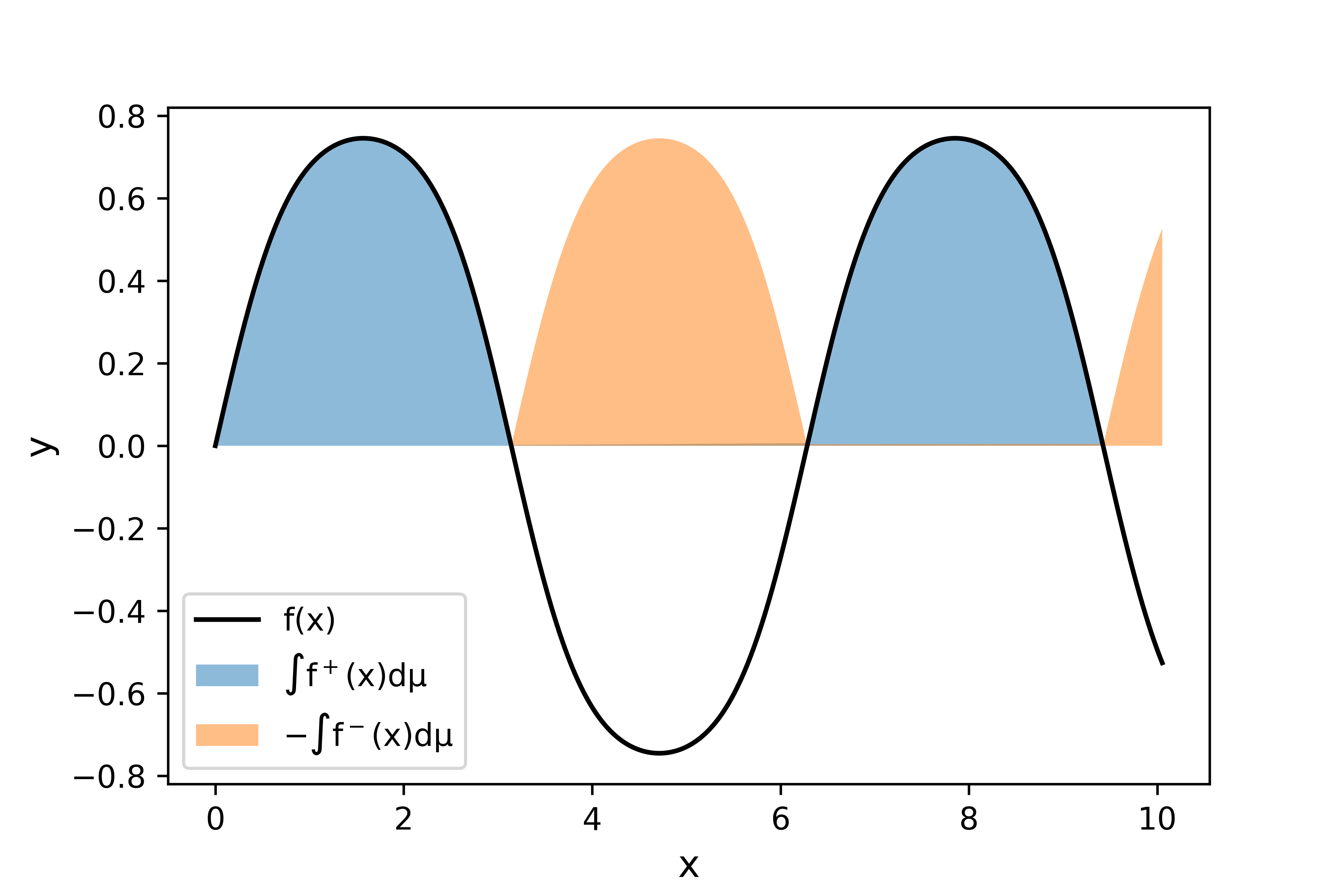
Figure 40: Example of a decomposition of a bounded, measurable function into $f^{+}$ and $f^{-}$. The Lebesgue integral is then just the integral of the blue region minus the integral of the orange region.

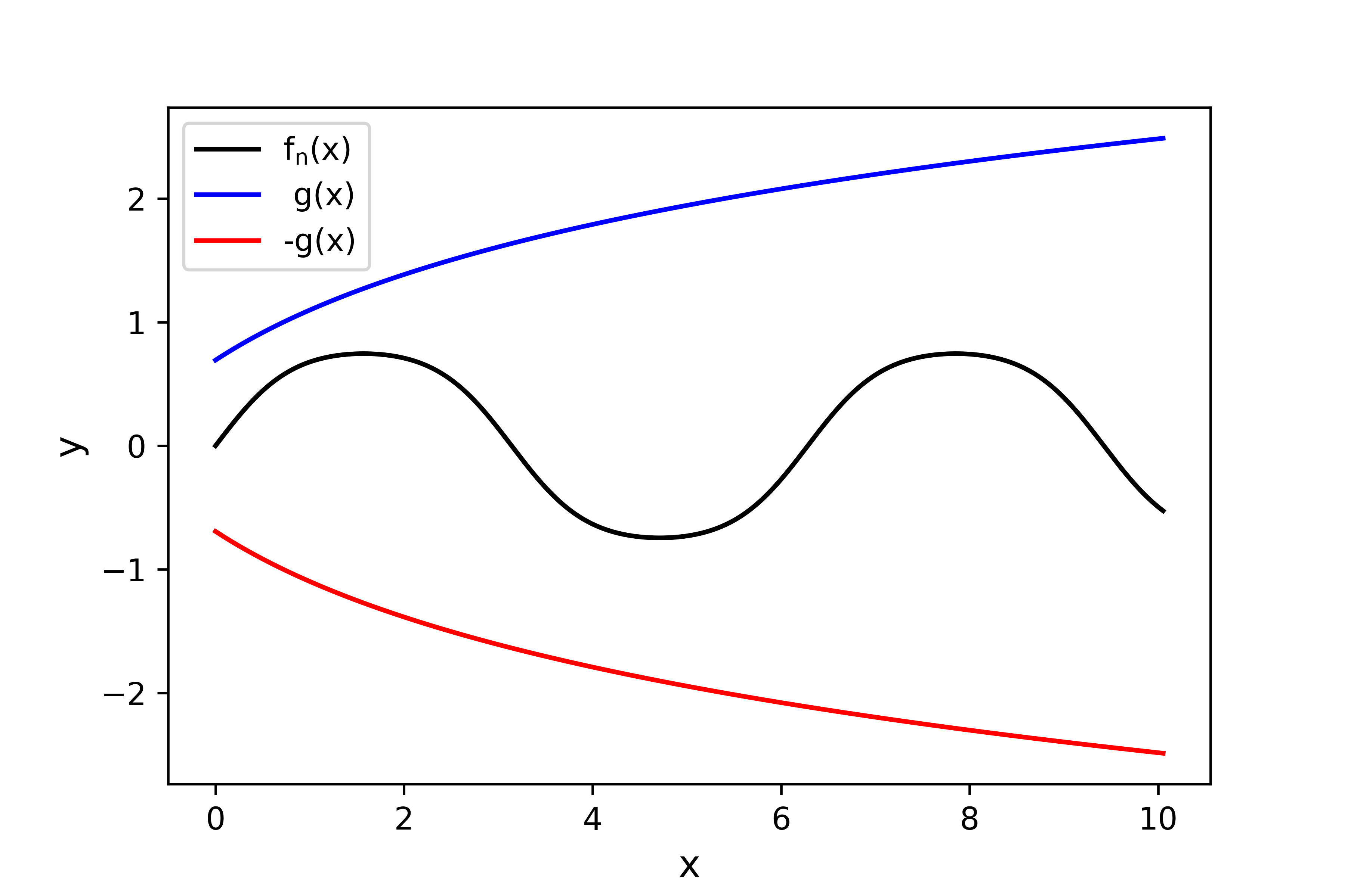
Figure 41: If $g$ is a non-negative, measurable function such that $\int gd\mu<\infty$ and $g$ dominates $f_{n}\rightarrow f$ pointwise almost everywhere ($\absolutevalue{f_{n}}\leq_{a.e.}g$), then $f$ and even $f_{i}$ are integrable.

$L^{P}(M,\sigma,\mu)$ Function Spaces

Define the set, $\mathcal{L}^{P}:=\{f:M\rightarrow\mathbb{C}|f\;\text{measurable},\int|f|^{p}d\mu<\infty\}$. If we equip $\mathcal{L}^{P}$ with pointwise addition and scalar multiplication then clearly $\mathcal{L}^{P}$ is a $\mathbb{C}$ vector space. One can then construct a map $\{\{\cdot\}\}_{p}:\mathcal{L}^{P}\rightarrow\mathbb{R}$ such that,

$$\{\{f\}\}_{p}=\bigg{(}\int|f|^{p}d\mu\bigg{)}^{1/p}$$ (363)

where $p\in\mathbb{R}$ and $1\leq p<\infty$ that is a semi-norm with the following properties:

1. $\forall\alpha\in\mathbb{C}$ then $\{\{\alpha f\}\}_{p}=|\alpha|\cdot_{\mathbb{C}}\{\{f\}\}_{p}$

2. $\forall f,g\in\mathcal{L}^{P}$ then $\{\{f+_{\mathcal{L}}g\}\}_{p}\leq\{\{f\}\}_{p}+_{\mathbb{C}}\{\{g\}\}_{p}$

3. $\{\{f\}\}_{p}\geq 0$ and $\{\{f\}\}_{p}=0$ implies $f=_{a.e.}0$

Notice that for a norm, we must have that the last condition is satisfied everywhere (not almost everywhere). Therefore, $\mathcal{L}^{P}$ is not even a normed space. However, we can use equivalence classes to remove troublesome functions in $\mathcal{L}^{P}$ that are zero almost everywhere while refusing to be zero everywhere. First, we can define the equivalence relation between $f,g\in\mathcal{L}^{P}$ as equivalent if,

$$f\sim g:<=>f=_{a.e.}g.$$ (364)

Equivalence relations are interesting since they allow us to split up a space according to equivalent classes of objects within the set. We define the quotient space of a set, $M/\sim$ to be the set of all $m\in M$ for which $m_{i}\sim m_{j}$. If we take an equivalence class on $\mathcal{L}^{P}$ to be those functions satisfying Equation (364), then we define a new space $L^{P}$ such that,

$$L^{P}=\mathcal{L}^{P}/\sim=\{[f]_{\sim}|f\in\mathcal{L}^{P}\}.$$ (365)

Although we will not explicitly prove this, $L^{P}$ inherits a norm from $\mathcal{L}^{P}$ such that,

$$\norm{\cdot}_{p}:L^{P}\rightarrow\mathbb{R}$$ (366)

$$[f]_{\sim}\rightarrow\norm{[f]_{\sim}}_{p}:=\{\{f\}\}_{p}.$$ (367)

It can the be shown that $L^{P}$ is in fact a Banach space, and by the Holder inequality it is even a Hilbert space for $p=2$ (the inner product is sesqui-linear). In fact, all of quantum mechanics of a particle in three dimensions rests on the $L^{2}(\mathbb{R}^{3},\sigma(\mathcal{O}_{\mathbb{R}}),\lambda^{3})$ Hilbert space.

D.1.3 Adjoints

The adjoint $A^{*}:\mathcal{D}_{A^{*}}\rightarrow\mathcal{H}$ of a densely defined operator $A:\mathcal{D}_{A}\rightarrow\mathcal{H}$ is defined such that,

$$\mathcal{D}_{A^{*}}:=\{\psi\in\mathcal{H}|\forall\alpha\in\mathcal{D}_{A}\;\exists\eta\in\mathcal{H}:\;(\psi,A\alpha)=(\eta,\alpha)\}$$ (368)

where the operator $A^{*}\psi=\eta$. Prove that $A\subseteq B$ implies that $B^{*}\subseteq A^{*}$.

Proof.

$A\subseteq B$ implies that $\mathcal{D}_{A}\subseteq\mathcal{D}_{B}$ and $\forall\alpha\in\mathcal{D}_{A}$ $B$ acts on $\alpha$ in the same manner: $A\alpha=B\alpha$. Let $\psi\in\mathcal{D}_{B^{*}}$. Then $\forall\alpha\in\mathcal{D}_{A}\subseteq\mathcal{D}_{B}$ we have,

$$(\psi,B\alpha)=(\psi,A\alpha).$$ (369)

But by the definition of $\mathcal{D}_{A^{*}}$,

$$\mathcal{D}_{A^{*}}:=\{\psi\in\mathcal{H}|\forall\alpha\in\mathcal{D}_{A}\;\exists\eta\in\mathcal{H}:\;(\psi,A\alpha)=(\eta,\alpha)\}$$ (370)

we must have that $\psi\in\mathcal{D}_{A^{*}}$. This implies that $\mathcal{D}_{B^{*}}\subseteq\mathcal{D}_{A^{*}}$ and $B^{*}\subseteq A^{*}$. ∎

A densely defined operator is called symmetric (in physics literature, Hermitian) if $\forall\alpha,\beta\in\mathcal{D}_{A}:\;(\alpha,A\beta)=(A\alpha,\beta)$. We can easily show that if a densely defined operator $A$ is symmetric that its adjoint is an extension $A\subseteq A^{*}$.

Proof.

Let $A:\mathcal{D}_{A}\rightarrow\mathcal{H}$ be a symmetric opertor such that, $\forall\alpha,\beta\in\mathcal{D}_{A}:\;(\alpha,A\beta)=(A\alpha,\beta)$. Then let $\psi\in\mathcal{D}_{A}$. By the definition of $\mathcal{D}_{A^{*}}$,

$$\mathcal{D}_{A^{*}}:=\{\psi\in\mathcal{H}|\forall\alpha\in\mathcal{D}_{A}\;\exists\eta\in\mathcal{H}:\;(\psi,A\alpha)=(\eta,\alpha)\}$$ (371)

we must have that $\psi\in\mathcal{D}_{A^{*}}$ so that $\mathcal{D}_{A}\subseteq\mathcal{D}_{A^{*}}$. Since $A$ is symmetric, we also have that $A^{*}\psi=A\psi$ so that $A\subseteq A^{*}$. ∎

A self-adjoint operator is an operator that is equal to its adjoint, $A=A^{*}$. An interesting property of self-adjoint operators are that they cannot be further extended to some other operator. To see this,

Proof.

Assume that $B$ is a self-adjoint extension of $A$. Then,

$$A\subseteq B=B^{*}\subseteq A^{*}=A.$$ (372)

∎

The notion of closable, closure, and closed are important to understanding the behavior of operators. We introduce the following three definitions:

1. Closable: A densely defined operator is closeable if its adjoint $A^{*}$ is also densely defined.

2. The closure of a closeable operator $A$ is $A^{**}$.

3. An operator $A$ is closed if $A=A^{**}$.

Show that if $A$ is symmetric that $A^{**}\subseteq A^{*}$.

Proof.

A symmetric means that $A\subseteq A^{*}$. But by our previous result we know that $A^{**}\subseteq A^{*}$ and we are done. ∎

A symmetric operator $A$ is called essentially self-adjoint if its closure $A^{**}$ is self-adjoint. An interesting result is that for an essentially self-adjoint operator $A$ the closure $A^{**}$ is the unique self-adjoint extension of $A$.

Proof.

We know that $A\subseteq A^{**}$ by our previous theorem. Assume there is some other self-adjoint extension $B$ so that $A\subseteq B=B^{*}$. But then $B^{**}\subseteq A^{*}$ or equivalently $A^{**}\subseteq B^{***}=B$. But since $A^{**}$ cannot be further extended we must have that $B=A^{**}$. ∎

We can quickly check if a symmetric operator $A$ has self-adjoint extensions by evaluating its defect indices. If the defect indices coincide, then there are self-adjoint extensions of $A$, and if they are different there are none. For the special case where both defect indices are zero, there exists a unique such extension.

$$d_{+}=\text{dim}(\text{ker}(A^{*}-i))$$ (373)

$$d_{-}=\text{dim}(\text{ker}(A^{*}+i)).$$ (374)

D.1.4 The Spectral Theorem

As we will see in the axioms of quantum mechanics, the possible measurement values are those in the spectrum, $\sigma(A)$ of an observable $A$. A common task in any quantum mechanical calculation is to determine the spectra of one or several self-adjoint operators. In this section, we will first introduce important definitions related to the spectra of operators and then proceed to the spectral theorem.

The Resolvent Set and Spectrum

First, define the resolvent map of a closed operator $A=A^{**}$ as the map,

$$R_{A}:\rho(A)\rightarrow\mathcal{L}(\mathcal{H},\mathcal{H})$$ (375)

$$z\in\mathbb{C}\longmapsto(A-z\cdot id_{\mathcal{D}_{A}})^{-1}$$ (376)

where $\rho(A)\subseteq\mathbb{C}$ is known as the resolvent set. Hence, the resolvent set is all the complex numbers where $(A-z\cdot id_{\mathcal{D}_{A}})^{-1}$ exists and is a bounded linear map from $\mathcal{H}\rightarrow\mathcal{H}$. The complement of the resolvent set is called the spectrum, $\sigma(A)=\mathbb{C}\backslash\rho(A)$. This means that the spectrum is just the set of complex numbers where $(A-z\cdot id_{\mathcal{D}_{A}})^{-1}$ does not exist. The spectrum of an operator on a finite dimensional vector space is precisely equal to the set of eigenvalues, but for infinite dimension spaces this is not necessarily the case. All that we know is that if the eigenvalues of the self-adjoint operator exist, they must be in the spectrum.

We define the total spectra $\sigma(A)$ as the union of pure point, point imbedded in a continuum and purely continuous spectra such that,

$$\sigma(A)=\sigma_{pp}\cup\sigma_{pic}\cup\sigma_{pc}$$ (377)

with precise definitions given by,

1. $\sigma_{pp}:=\{z\in\mathbb{C}|ran(A-z)=\overline{ran(A-z)}\neq\mathcal{H}\}$

2. $\sigma_{pic}:=\{z\in\mathbb{C}|ran(A-z)\neq\overline{ran(A-z)}\neq\mathcal{H}\}$

3. $\sigma_{pc}:=\{z\in\mathbb{C}|ran(A-z)\neq\overline{ran(A-z)}=\mathcal{H}\}$

We now arrive at an important theorem.

Theorem D.9.

The point spectrum of a self-adjoint operator $A$ has as its elements precisely the eigenvalues of $A$.

Proof.

First, show that if $\lambda$ is an eigenvalue of $A$ then $\lambda\in\mathbb{R}$. Consider, for $A\psi=\lambda\psi$, that,

$$\lambda(\psi,\psi)=(\psi,\lambda\psi)=(\psi,A\psi).$$ (378)

But if $A$ is self-adjoint, we have,

$$(\psi,A\psi)=(A\psi,\psi)=\overline{(\psi,A\psi)}=\overline{(\psi,\lambda\psi)}=\overline{\lambda}\overline{(\psi,\psi)}=\overline{\lambda}(\psi,\psi).$$ (379)

Of course, since $\psi\neq 0$ we must have $\lambda=\overline{\lambda}$ which implies $\lambda\in\mathbb{R}$. Now suppose that $\lambda$ is indeed an eigenvalue of $A$. Then,

$$\text{ker}(A-\lambda)\neq\{0\}_{\mathcal{H}}.$$ (380)

But then,

$$\text{ker}(A-\lambda)=\text{ker}(A^{*}-\lambda)=\text{ker}((A-\overline{\lambda})^{*})=\text{ran}(A-\overline{\lambda})^{\perp}=\text{ran}(A-\lambda)^{\perp}$$ (381)

which implies that,

$$(\text{ran}(A-\lambda)^{\perp})^{\perp}=\overline{\text{ran}(A-\lambda)}\neq\{0\}^{\perp}_{\mathcal{H}}=\mathcal{H}$$ (382)

which by definition means that $\lambda\in\sigma_{pp}(A)$. Conversely, suppose that $\lambda\in\mathbb{C}$ is not an eigenvalue of $A$. Then $\overline{\lambda}$ is not an eigenvalue either. By a manner similar to the previous statement we obtain,

$$\text{ker}(A-\lambda)=\{0\}_{\mathcal{H}}$$ (383)

$$(\text{ran}(A-\lambda)^{\perp})^{\perp}=\overline{\text{ran}(A-\lambda)}=\{0\}^{\perp}_{\mathcal{H}}=\mathcal{H}$$ (384)

which means that $\lambda\notin\sigma_{pp}(A)$ and we are done. ∎

Projection-Valued Measures

A projection-valued measure (PVM) is a map from the Borel $\sigma$-algebra on the reals to the bounded linear maps on a Hilbert space, $P:\sigma(\mathcal{O}_{\mathbb{R}})\rightarrow\mathcal{L}(\mathcal{H},\mathcal{H})$, that satisfies the following properties:

1. $\forall\Omega\in\sigma(\mathcal{O}_{\mathbb{R}})$, $P(\Omega)^{*}=P(\Omega)$

2. $\forall\Omega\in\sigma(\mathcal{O}_{\mathbb{R}})$, $P(\Omega)\circ P(\Omega)=P(\Omega)$

3. $P(\mathbb{R})=id_{\mathcal{H}}$

4. $\forall\Omega\in\sigma(\mathcal{O}_{\mathbb{R}})\ni\Omega=\sqcup_{n\geq 1}\Omega_{n}$ implies $\forall\psi\in\mathcal{H}:\sum_{n\geq 1}(P(\Omega_{n})\psi)=P(\Omega)\psi$

Many of the useful properties of PVMs are listed below:

1. $P(\emptyset)=0_{\mathcal{H}}$ where $0_{\mathcal{H}}:\mathcal{H}\rightarrow\mathcal{H}$ which takes an element in the Hilbert space and returns the 0 on $\mathcal{H}$.

2. $P(\mathbb{R}\backslash\Omega)=id_{\mathcal{H}}-P(\Omega)$

3. $P(\Omega_{1}\cup\Omega_{2})+P(\Omega_{1}\cap\Omega_{2})=P(\Omega_{1})+P(\Omega_{2})$

4. $P(\Omega_{1}\cap\Omega_{2})=P(\Omega_{1})\circ P(\Omega_{2})$

5. $\Omega_{1}\subseteq\Omega_{2}$ implies $\text{ran}(P(\Omega_{1}))\subseteq\text{ran}(P(\Omega_{2}))$

Finally, one piece of notation that we will find useful is that $P(\lambda):=P((-\infty,\lambda])$. Recall that $P$ takes an element of the Borel $\sigma$-algebra which is generated by the half open intervals $(-\infty,\lambda]$.

Now, we introduce the concept that a PVM can be used to define complex- and real-valued Borel measures. For instance, a complex-valued Borel measure can be induced such that,

$$\forall\psi,\phi\in\mathcal{H},\;\mu_{\psi,\phi}:\sigma(\mathcal{O}_{\mathbb{R}})\rightarrow\mathbb{C}$$ (385)

where $\mu_{\psi,\phi}$ maps an element $\Omega$ of the Borel-$\sigma$-algebra into the inner product $(\psi,P(\Omega)\phi)$,

$$\Omega\rightarrow\mu_{\psi,\phi}:=(\psi,P(\Omega)\phi).$$ (386)

Trivially, a real-valued Borel measure can be induced $\forall\psi\in\mathcal{H}$ so that, $\mu_{\psi}:=\mu_{\psi,\psi}$.

We now proceed to discuss integration of PVMs for simple, bounded and unbounded measurable functions $f:\mathbb{R}\rightarrow\mathbb{C}$.

Integration of Simple Functions: Recall that $f:\mathbb{R}\rightarrow\mathbb{C}$ is called simple if it has a decomposition $f(\mathbb{R})=\{f_{1},...,f_{n}\}\subseteq\mathbb{C}$ such that,

$$f=\sum_{n=1}^{N}f_{n}\cdot\chi_{preim_{f}}(\{f_{n}\})$$ (387)

where clearly the function $f$ can be written as a sum of complex-values by their respective characteristic functions on the pre-image of $f$. The integral of such a function with respect to a PVM is defined as,

$$\int_{\mathbb{R}}fdP:=\sum_{n=1}^{N}f_{n}\cdot P(\text{preim}_{f}(\{f_{n}\}))$$ (388)

which is easily observed to have the following properties:

1. For any $\chi_{\Omega}$ with $\Omega\in\sigma(\mathcal{O}_{\mathbb{R}})$ the integral over $\chi_{\Omega}$ is just the PVM acting on $\Omega$ so that,

   $$\int_{\mathbb{R}}\chi_{\Omega}dP=P(\Omega).$$ (389)

2. $\forall\psi,\phi\in\mathcal{H}$,

   $$\begin{split}(\psi,\bigg{(}\int_{\mathbb{R}}fdP\bigg{)}\phi)=&(\psi,\sum_{n=1}^{N}f_{n}\cdot P(\Omega_{n})\phi)\\ =&\sum_{n=1}^{N}f_{n}(\psi,P(\Omega_{n})\phi)\\ =&\sum_{n=1}^{N}f_{n}\cdot\mu_{\psi,\phi}(\Omega_{n})\\ =&\int_{\mathbb{R}}fd\mu_{\psi,\phi}.\end{split}$$ (390)

Integration of Bounded Borel Functions: Consider the Banach space of measurable functions $B(\mathbb{R}):=\{f:\mathbb{R}\rightarrow\mathbb{C}|\norm{f}_{\infty}<\infty\}$. Note that the space of simple measurable functions from the real to complex numbers is a dense subset of $B(\mathbb{R})$, which means that there exists a unique extension of $\int dP$ to $B(\mathbb{R})$ by the Bounded Linear Transformation theorem,

$$\int dP:\overbrace{B(\mathbb{R})}^{\text{Banach}}\rightarrow\overbrace{\mathcal{L}(\mathcal{H},\mathcal{H})}^{\text{Banach}}$$ (391)

with the following properties:

1. $\int_{\mathbb{R}}1dP=id_{\mathcal{H}}$

2. $\int_{\mathbb{R}}(f\cdot g)dP=\int_{\mathbb{R}}fdP\circ\int_{\mathbb{R}}gdP$

3. $\int_{\mathbb{R}}\overline{f}dP=(\int_{\mathbb{R}}fdP)^{*}$

The first two properties can be called a $C^{*}$-algebra homomorphism.

Integration of Unbounded Borel Functions: The integral over the PVM has been shown to send a bounded Borel function to a bounded, linear operator $\int fdP$. However, we will now define a construction that also applies to unbounded Borel functions. Let $f:\mathbb{R}\rightarrow\mathbb{C}$ be a measureable, unbounded Borel function. Define the linear map,

$$\int fdP:\mathcal{D}_{\int_{\mathbb{R}fdP}}\subseteq\mathcal{H}\rightarrow\mathcal{H}$$ (392)

be defined on the dense linear subset $\mathcal{D}_{\int_{\mathbb{R}fdP}}:=\{\psi\in\mathcal{H}|\int\absolutevalue{f}^{2}d\mu_{\psi}<\infty\}$ which takes an element $\psi\in\mathcal{H}$ to its integral,

$$\psi\mapsto\bigg{(}\int fdP\bigg{)}\psi:=\lim_{n\to\infty}\bigg{[}\bigg{(}\int_{\mathbb{R}}f_{n}dP\bigg{)}\psi\bigg{]}$$ (393)

where the $f_{n}:=\chi_{\{x\in\mathbb{R}|\absolutevalue{f(x)}\leq n\}}f$. Since the integral is Cauchy in $\mathcal{H}$, the integral has the following properties:

1. $\bigg{(}\int fdP\bigg{)}^{*}=\int\overline{f}dP$.

2. $\forall\alpha\in\mathbb{C}$, we have,

   $$\alpha\int fdP+\int gdP\subseteq\int(\alpha f+g)dP$$ (394)

   with equality when $f,g$ are bounded. If $f,g$ are unbounded then the right-hand side is an extension of the left-hand side.

3. $(\int fdP)\circ(\int gdP)\subseteq\int(f\circ g)dP$ with equality when $f,g$ are bounded.

The Inverse Spectral Theorem: The inverse spectral theorem can now be stated as a precursor to the proof of the spectral theorem. Given a PVM, $P$, we can construct a self-adjoint operator,

$$A_{P}:=\int id_{\mathbb{R}}dP$$ (395)

since,

$$A_{P}^{*}=\bigg{(}\int id_{\mathbb{R}}dP\bigg{)}^{*}=\int\overline{id_{\mathbb{R}}}dP=\int id_{\mathbb{R}}dP=A_{P}.$$ (396)

Now we want to go backwards from the previous result; namely, we want to actually find this $P$ given some self-adjoint operator $A$. First we introduce the concept of spectrally decomposable self-adjoint operators. $A$ self-adjoint is called spectrally decomposable if there exists a projection-valued measure $P$ such that,

$$A=\int id_{\mathbb{R}}dP$$ (397)

like what we have in the inverse spectral theorem. Then for any measurable $f:\mathbb{R}\rightarrow\mathbb{R}$ we define the application of the real-valued function to the spectrally decomposable self-adjoint operator as,

$$f(A):=\int f(\lambda)P(d\lambda)=\int f\circ id_{\mathbb{R}}dP$$ (398)

with,

$$f(A):\mathcal{D}_{\int fdP}\rightarrow\mathcal{H}$$ (399)

where the domain is given by,

$$\mathcal{D}_{\int fdP}=\{\psi\in\mathcal{H}|\int|f|^{2}d\mu_{\psi}\}$$ (400)

and $\mu_{\psi}$ is the real-valued Borel measure induced by $(\psi,P(\Omega)\psi)$.

But how do we reconstruct a projection-valued measure from a spectrally decomposed self-adjoint operator? Let $A=\int_{\mathbb{R}}\lambda P(d\lambda)$ for some projection-valued measure $P$. Then the resolvent $R_{A}(z)$ for $z\in\rho(A)\subseteq\mathbb{C}$ can be written as,

$$R_{A}(z)=(A-zid_{\mathcal{H}})^{-1}=r_{z}(A)=\int_{\mathbb{R}}r_{z}dP$$ (401)

where $r_{z}(A)$ is a function from $r_{z}(A):\mathbb{C}\to\mathbb{C}$ takes some complex number $\lambda\to\frac{1}{\lambda-z}$. Then $\forall\psi\in\mathcal{H}$, we can write,

$$(\psi,R_{A}(z)\psi)=\int_{\mathbb{R}}r_{z}d\mu_{\psi}=\int_{\mathbb{R}}\frac{1}{\lambda-z}d\mu_{\psi}.$$ (402)

Such a function has special properties since it is a Herglotz function, that is, that it maps the upper half of the complex plane into itself,

$$(\psi,R_{A}(z)\psi):\mathbb{C}^{+}\to\mathbb{C}^{+}$$ (403)

where $\mathbb{C}^{+}:=\{z\in\mathbb{C}|\imaginary(z)\geq 0\}$. This allows us to reconstruct a real-valued Borel measure from the object $(\psi,R_{A}(z)\psi)\geq 0$. To see this, consider that,

$$\lim_{\epsilon\to 0^{+}}\frac{1}{\pi}\int_{t_{1}}^{t_{2}}dt\imaginary(\psi,R_{A}(t+i\epsilon)\psi)=\lim_{\epsilon\to 0^{+}}\frac{1}{\pi}\int_{t_{1}}^{t_{2}}dt\int_{\mathbb{R}}\frac{\epsilon}{\absolutevalue{\lambda-t-i\epsilon}^{2}}\mu_{\psi}(d\lambda)$$ (404)

where Fubini’s theorem allows us to exchange the integrals so that,

$$=\lim_{\epsilon\to 0^{+}}\frac{1}{\pi}\int_{\mathbb{R}}\int_{t_{1}}^{t_{2}}dt\frac{\epsilon}{\absolutevalue{(\lambda-t)^{2}+\epsilon^{2}}}\mu_{\psi}(d\lambda)=\lim_{\epsilon\to 0^{+}}\int_{\mathbb{R}}\frac{1}{\pi}\arctan{\bigg{(}\frac{t-\lambda}{\epsilon}}\bigg{)}\bigg{|}^{t_{2}}_{t_{1}}\mu_{\psi}(d\lambda)$$ (405)

which in the limit as $\epsilon\to 0$ is simply the sum of two characteristic functions (by virtue of the two competing $\arctan$ terms for $t_{1}$ and $t_{2}$),

$$\lim_{\epsilon\to 0^{+}}\frac{1}{\pi}\int_{t_{1}}^{t_{2}}dt\imaginary(\psi,R_{A}(t+i\epsilon)\psi)=\int_{\mathbb{R}}\frac{1}{2}(\chi_{(t_{1},t_{2})}+\chi_{[t1,t2]})\mu_{\psi}(d\lambda).$$ (406)

Thus, we have the following theorem:

Theorem D.10.

Stieltjes Inversion Formula: For Herglotz functions $\mu_{\psi}:\sigma(\mathcal{O}_{\mathbb{R}})\to\mathbb{R}^{+}_{0}$, we can recover the real Borel measure from the resolvent set using,

$$\mu((-\infty,\lambda])=\lim_{\delta\to 0^{+}}\lim_{\epsilon\to 0^{+}}\frac{1}{\pi}\int_{-\infty}^{\lambda+\delta}dt\imaginary(\psi,R_{A}(t+i\epsilon)\psi).$$ (407)

Proof.

The right hand side is just,

$$=\lim_{\delta\to 0^{+}}\int_{\mathbb{R}}\frac{1}{2}(\chi_{(-\infty,\lambda+\delta)}+\chi_{[-\infty,\lambda+\delta]})\mu_{\psi}(d\lambda)$$ (408)

which by the theorem of dominant convergence is just,

$$=\int_{\mathbb{R}}(\chi_{(-\infty,\lambda]})\mu_{\psi}(d\lambda)$$ (409)

just gives us $\mu((-\infty,\lambda])$ by definition. ∎

Up to this point, we know that given some spectrally decomposable, self-adjoint operator $A=\int_{\mathbb{R}}id_{\mathbb{R}}dP$, that $P$ can be recovered from $A$ by virtue of $(\psi,P(\Omega)\phi)=\int\chi_{\Omega}d\mu_{\psi,\phi}$ where $\mu_{\psi,\phi}$ is the complex Borel measure.

Theorem D.11.

The Spectral Theorem: For any self-adjoint operator $A:\mathcal{D}_{A}\to\mathcal{H}$, there is a unique projection-valued measure $P_{A}:\sigma(\mathcal{O}_{\mathbb{R}})\to\mathcal{L}(\mathcal{H}\to\mathcal{H})$, such that $A=\int_{\mathbb{R}}id_{\mathcal{H}}dP_{A}$.

Proof.

To construct a projection-valued measure from a self-adjoint operator, it thus remains to show that $(\psi,R_{A}(\cdot)\psi)$ is Herglotz for any self-adjoint operator $A$, that $(\psi,P(\Omega)\phi):=\int\chi_{\Omega}d\mu_{\psi,\phi}$ is indeed a projection-valued measure, and that this projection-valued measure is unique. We will first begin by proving a few lemmas that will be useful later in the proof.

Lemma D.1.

The First Resolvent Formula: For any operator $A:\mathcal{D}_{A}\to\mathcal{H}$ and $a,b\in\mathbb{C}\in\rho(A)$, we have,

$$R_{A}(a)-R_{B}(b)=(a-b)R_{A}(a)\circ R_{A}(b)$$ (410)

or equivalently,

$$R_{A}(a)-R_{B}(b)=(a-b)R_{A}(b)\circ R_{A}(a).$$ (411)

Proof.

Note that,

$$(A-a)^{-1}-(a-b)(A-a)^{-1}(A-b)^{-1}=(A-a)^{-1}(id_{\mathcal{H}}-(a-b)(A-b)^{-1})$$ (412)

which is of course,

$$(A-a)^{-1}(id_{\mathcal{H}}-(a+A-A-b)(A-b)^{-1})=(A-a)^{-1}(A-a)(A-b)^{-1}=(A-b)^{-1}$$ (413)

which proves this first assertion known as the "first resolvent formula".

∎

Lemma D.2.

$(\psi,R_{A}(\cdot)\psi)$ is Herglotz for any self-adjoint operator $A$.

Proof.

Let $z\in\mathbb{C}^{+}$ and $F(z)=(\psi,R_{A}(\cdot)\psi)=\int_{\mathbb{R}}\frac{1}{\lambda-z}d\mu_{\psi}$. Then just notice that,

$$\imaginary F(z)=\imaginary z\int_{\mathbb{R}}\frac{1}{\absolutevalue{\lambda-z}^{2}}d\mu_{\psi}\in\mathbb{C}^{+}.$$ (414)

∎

Lemma D.3.

$(\psi,P(\Omega)\phi):=\int\chi_{\Omega}d\mu_{\psi,\phi}$ is a unique projection-valued measure constructed from $A$.

Proof.

The Stieltjes inversion formula can provide a unique real Borel measure from the resolvent set, from which $(\psi,P(\Omega)\phi)$ is uniquely determined. ∎

Putting all of this together, we can prove the spectral theorem in its entirety. First, we can define a real-valued Borel measure $\forall\psi\in\mathcal{H}$ such that,

$$\mu_{\psi}^{A}:\sigma(\mathcal{O}_{\mathbb{R}})\to\mathbb{R}$$ (415)

$$\mu_{\psi}^{A}((-\infty,\lambda]):=\lim_{\delta\to 0^{+}}\lim_{\epsilon\to 0^{+}}\frac{1}{\pi}\int_{-\infty}^{\lambda+\delta}dt\imaginary(\psi,R_{A}(t+i\epsilon)\psi)$$ (416)

since $\mu_{\psi}^{A}$ is Herglotz (Lemma D.1) and where $R_{A}$ is the resolvent map which takes an complex element of the resolvent set to a bounded linear map on $\mathcal{H}$ in the following way,

$$R_{A}:\rho(A)\to\mathcal{L}(\mathcal{H})$$ (417)

$$R_{A}(z):=(A-zid_{\mathcal{H}})^{-1}.$$ (418)

Then, we construct a complex-valued Borel measure via the polarization formula such that $\forall\psi,\phi\in\mathcal{H}$ and all Borel sets $\Omega\in\sigma(\mathcal{O}_{\mathbb{R}})$,

$$\mu_{\psi,\phi}:\sigma(\mathcal{O}_{\mathbb{R}})\to\mathbb{C}$$ (419)

$$\mu_{\psi,\phi}(\Omega):=\frac{1}{4}[\mu_{\psi+\phi}(\Omega)-\mu_{\psi-\phi}(\Omega)+i\mu_{\psi-i\phi}(\Omega)-i\mu_{\psi+i\phi}(\Omega)].$$ (420)

Finally, we can define the unique projection-valued measure (Lemma D.2) such that $\forall\psi,\phi\in H$,

$$P_{A}:\sigma(\mathcal{O}_{\mathbb{R}})\to\mathcal{L}(\mathcal{H})$$ (421)

$$(\psi,P_{A}(\Omega)\phi):=\int\chi_{\Omega}d\mu_{\psi,\phi}$$ (422)

where $\chi$ is the characteristic function. Thus, we have constructed the unique projection-valued measure from a self-adjoint operator and we are done.

∎

The consequences of the spectral theorem to quantum theory are immensely important. First, we will take as an axiom that the observables of a quantum mechanical system are given by the self-adjoint linear maps on the Hilbert space associated with a quantum system. Then, the probability of the system being in some state $\rho$ is defined as the trace of the unique projection-valued measure $P_{A}$ induced by self-adjoint operator $A$ composed with $\rho$. The only remaining axioms related to unitary and projective quantum dynamics serve to evolve the quantum system in time and "collapse" the system into some observation at measurement time $t_{m}$, respectively.

D.2 An Axiomatic Approach to Quantum Mechanics

Axiom 1.

With every quantum system there is associated a complex Hilbert space $(\mathcal{H},+,\cdot,(\cdot,\cdot))$, with states that are all positive, trace-class, linear maps $\rho:\mathcal{H}\rightarrow\mathcal{H}$ for which $Tr(\rho)=1$

The Hilbert space is equipped with addition, scalar multiplication, and a sesqui-linear inner product (Hermitian, linear, and non-negative) and is complete.

Axiom 2.

The observables of a quantum system are the self-adjoint linear maps $A:\mathcal{D}_{A}\rightarrow\mathcal{H}$ where $\mathcal{D}_{A}$ is some densely defined subset of $\mathcal{H}$. Self-adjointness is defined so that the map $A$ coincides with its adjoint map $A^{*}$ so that,

$$\mathcal{D}_{A^{*}}:=\{\psi\in\mathcal{H}|\forall\alpha\in\mathcal{D}_{A}\;\exists\nu\in\mathcal{H}:\;(\psi,A\alpha)=(\nu,\alpha)\}$$ (423)

$$A^{*}(\psi)=\nu.$$ (424)

Axiom 3.

The probability that a measurement of an observable A on a system is in the state $\rho$ yields the result in the Borel set $E\subset\mathbb{R}$ is given by,

$$\mu_{\rho}^{A}(E):=Tr(P_{A}(E)\circ\rho)$$ (425)

where $P_{A}(E)$ is the unique projection-valued measure that is associated with a self-adjoint linear map $A$ according to the spectral theorem. Furthermore, the composition $P_{A}(E)\circ\rho$ is again trace-class.

Axiom 4.

Unitary dynamics occur during time intervals $(t_{1},t_{2})$ during which no measurement occurs such that,

$$\rho(t_{2})=\mathcal{U}(t_{2}-t_{1})\rho(t_{1})\mathcal{U}^{-1}(t_{2}-t_{1})$$ (426)

where the time evolution operator is written as $\mathcal{U}(t)=e^{\frac{-i\mathcal{H}t}{\hbar}}$.

Axiom 5.

Projective dynamics occur when a measurement is made at some time, $t_{m}$. Then the state immediately after the measurement of an observable $A$ is,

$$\rho_{after}:=\frac{P_{A}(E)\rho_{before}P_{A}(E)}{Tr(P_{A}(E)\rho_{before}P_{A}(E))}.$$ (427)

The idea is just to find some self-adjoint operator that corresponds to a physical observable, use the spectral theorem to find a unique projection-valued measure, and then calculate the probability of the observation, time-evolution of the system, and projective dynamics of the system according to these axioms. The content of quantum theory then is to construct self-adjoint operators that correspond to physical observables / experimental measurements. This task is non-trivial and forms the basis of all of quantum theory.

References

- [1] Clive A. Croxton “Liquid State Physics” Cambridge University Press, 2009 URL: https://ui.adsabs.harvard.edu/abs/2009lsp..book.....C
- [2] J.. Yarnell, M.. Katz, R.. Wenzel and S.. Koenig “Structure Factor and Radial Distribution Function for Liquid Argon at 85K” In Phys. Rev. A 7.6, 1973, pp. 2130–2144 DOI: 10.1103/PhysRevA.7.2130
- [3] B… Willis and C.. Carlile “Experimental Neutron Scattering” Oxford University Press, 2017
- [4] A.K. Soper “Inelasticity corrections for time-of-flight and fixed wavelength neutron diffraction experiments” In Mol. Phys. 107.16, 2009, pp. 1667–1684 DOI: 10.1080/00268970903025667
- [5] R. Kubo “The fluctuation-dissipation theorem” In Reports on Progress in Physics 29.1, 1966, pp. 255 DOI: 10.1088/0034-4885/29/1/306
- [6] D.S. Sivia “Elementary Scattering Theory: For X-ray and Neutron Users” New York: Oxford University Press, 2011 URL: https://oxford.universitypressscholarship.com/10.1093/acprof:oso/9780199228676.001.0001/acprof-9780199228676
- [7] Daniel P. Petersen and David Middleton “Sampling and reconstruction of wave-number-limited functions in N-dimensional euclidean spaces” In Information and Control 5.4, 1962, pp. 279–323 DOI: 10.1016/S0019-9958(62)90633-2
- [8] Jörg Neuefeind et al. “The Nanoscale Ordered MAterials Diffractometer NOMAD at the Spallation Neutron Source SNS” In Nucl. Instrum. Methods. Phys. Res. B. 287, 2012, pp. 68–75 DOI: 10.1016/j.nimb.2012.05.037
- [9] Salvatore Torquato “Hyperuniform states of matter” In Physics Reports 745, Hyperuniform States of Matter, 2018, pp. 1–95 DOI: 10.1016/j.physrep.2018.03.001
- [10] E. Lorch “Neutron diffraction by germania, silica and radiation-damaged silica glasses” In Journal of Physics C: Solid State Physics 2.2, 1969, pp. 229 DOI: 10.1088/0022-3719/2/2/305
- [11] A.. Soper and E.. Barney “On the use of modification functions when Fourier transforming total scattering data” In Journal of Applied Crystallography 45.6, 2012, pp. 1314–1317 DOI: 10.1107/S002188981203960X
- [12] A.. Soper and E.. Barney “Extracting the pair distribution function from white-beam X-ray total scattering data” Publisher: International Union of Crystallography In Journal of Applied Crystallography 44.4, 2011, pp. 714–726 DOI: 10.1107/S0021889811021455
- [13] M.. Bellissent-Funel et al. “Neutron diffraction of liquid neon and xenon along the coexistence line” In Phys. Rev. B 45.9, 1992, pp. 4605–4613 DOI: 10.1103/PhysRevB.45.4605
- [14] Lawrie B. Skinner et al. “Benchmark oxygen-oxygen pair-distribution function of ambient water from x-ray diffraction measurements with a wide Q-range” In The Journal of Chemical Physics 138.7, 2013, pp. 074506 DOI: 10.1063/1.4790861
- [15] J.. Proctor et al. “A comparison of different Fourier transform procedures for analysis of diffraction data from noble gas fluids” In Journal of Applied Physics 134.11, 2023, pp. 114701 DOI: 10.1063/5.0161033
- [16] LS Ornstein and F Zernike “Integral equation in liquid state theory” In Proc. Acad. Sci. Amsterdam. 17, 1914
- [17] Jean-Pierre Hansen and I.. McDonald “Theory of Simple Liquids: with Applications to Soft Matter” San Diego: Academic Press, 2013
- [18] D. Levesque, J.. Weis and L. Reatto “Pair Interaction from Structural Data for Dense Classical Liquids” In Phys. Rev. Lett. 54.5, 1985, pp. 451–454 DOI: 10.1103/PhysRevLett.54.451
- [19] Jianzhong Wu and Mengyang Gu “Perfecting Liquid-State Theories with Machine Intelligence” In The Journal of Physical Chemistry Letters 14.47, 2023, pp. 10545–10552 DOI: 10.1021/acs.jpclett.3c02804
- [20] F.. Carvalho and J.. Braga “Radial distribution function for liquid gallium from experimental structure factor: a Hopfield neural network approach” In Journal of Molecular Modeling 26.8, 2020, pp. 193 DOI: 10.1007/s00894-020-04436-y
- [21] Wenqian Chen, Peiyuan Gao and Panos Stinis “Physics-informed machine learning of the correlation functions in bulk fluids” In Physics of Fluids 36.1, 2024, pp. 017133 DOI: 10.1063/5.0175065
- [22] R.. Henderson “A uniqueness theorem for fluid pair correlation functions” In Phys. Lett. A 49.3, 1974, pp. 197–198 DOI: 10.1016/0375-9601(74)90847-0
- [23] Frigyes Riesz and Béla Sz.-Nagy “Functional Analysis” Courier Corporation, 2012
- [24] M. Shell “The relative entropy is fundamental to multiscale and inverse thermodynamic problems” In J. Chem. Phys. 129.14, 2008, pp. 144108 DOI: 10.1063/1.2992060
- [25] Martin Hanke “Well-Posedness of the Iterative Boltzmann Inversion” In J. Stat. Phys. 170.3, 2018, pp. 536–553 DOI: 10.1007/s10955-017-1944-2
- [26] F. Frommer, M. Hanke and S. Jansen “A note on the uniqueness result for the inverse Henderson problem” In Journal of Mathematical Physics 60.9, 2019, pp. 093303 DOI: 10.1063/1.5112137
- [27] Fabio Frommer and Martin Hanke “A variational framework for the inverse Henderson problem of statistical mechanics” In Letters in Mathematical Physics 112.4, 2022, pp. 71 DOI: 10.1007/s11005-022-01563-w
- [28] W. Schommers “Pair potentials in disordered many-particle systems: A study for liquid gallium” In Phys. Rev. A 28.6, 1983, pp. 3599–3605 DOI: 10.1103/PhysRevA.28.3599
- [29] Timothy C. Moore, Christopher R. Iacovella and Clare McCabe “Derivation of coarse-grained potentials via multistate iterative Boltzmann inversion” In The Journal of Chemical Physics 140.22, 2014, pp. 224104 DOI: 10.1063/1.4880555
- [30] Mohammad Shakiba and Alexey V. Akimov “Machine-Learned Kohn–Sham Hamiltonian Mapping for Nonadiabatic Molecular Dynamics” In Journal of Chemical Theory and Computation, 2024 URL: https://doi.org/10.1021/acs.jctc.4c00008
- [31] A.. Soper “Empirical potential Monte Carlo simulation of fluid structure” In Chem. Phys. 202.2, 1996, pp. 295–306 DOI: 10.1016/0301-0104(95)00357-6
- [32] Oliver S., Daniel T. and Karen J. “Liquid structure of the choline chloride-urea deep eutectic solvent (reline) from neutron diffraction and atomistic modelling” In Green Chemistry 18.9, 2016, pp. 2736–2744 DOI: 10.1039/C5GC02914G
- [33] Oliver S. Hammond, Daniel T. Bowron and Karen J. Edler “The Effect of Water upon Deep Eutectic Solvent Nanostructure: An Unusual Transition from Ionic Mixture to Aqueous Solution” In Angewandte Chemie 129.33, 2017, pp. 9914–9917 DOI: 10.1002/ange.201702486
- [34] T. F. et al. “The structures of liquid pyridine and naphthalene: the effects of heteroatoms and core size on aromatic interactions” In Phys. Chem. Chem. Phys. 20.4, 2018, pp. 2704–2715 DOI: 10.1039/C7CP06689A
- [35] A.. Soper “Tests of the empirical potential structure refinement method and a new method of application to neutron diffraction data on water” In Mol. Phys. 99.17, 2001, pp. 1503–1516 DOI: 10.1080/00268970110056889
- [36] Ciprian G. Pruteanu, John S. Loveday, Graeme J. Ackland and John E. Proctor “Krypton and the Fundamental Flaw of the Lennard-Jones Potential” In J. Phys. Chem. Lett. 13.35, 2022, pp. 8284–8289 DOI: 10.1021/acs.jpclett.2c02004
- [37] A.. Soper “On the uniqueness of structure extracted from diffraction experiments on liquids and glasses” In Journal of Physics: Condensed Matter 19.41, 2007, pp. 415108 DOI: 10.1088/0953-8984/19/41/415108
- [38] Leonid Pereyaslavets et al. “Accurate determination of solvation free energies of neutral organic compounds from first principles” In Nature Communications 13.1, 2022, pp. 414 DOI: 10.1038/s41467-022-28041-0
- [39] Andrew Gelman, John B. Carlin, Hal S. Stern and Donald B. Rubin “Bayesian Data Analysis” New York: ChapmanHall/CRC, 1995 DOI: 10.1201/9780429258411
- [40] Nils Lid Hjort, Chris Holmes, Peter Müller and Stephen G. Walker “Bayesian Nonparametrics” Cambridge University Press, 2010
- [41] Bruno De Finetti “Theory of Probability: A Critical Introductory Treatment” Wiley, 1979
- [42] Daniel M. Zuckerman and August George “Bayesian Mechanistic Inference, Statistical Mechanics, and a New Era for Monte Carlo” In Journal of Chemical Theory and Computation, 2024 DOI: 10.1021/acs.jctc.4c00014
- [43] Christopher M. Bishop “Pattern recognition and machine learning”, Information science and statistics New York: Springer, 2006
- [44] Jörg C. Lemm “Bayesian Field Theory” JHU Press, 2003
- [45] Bruno de Finetti “Theory of Probability: A Critical Introductory Treatment” John Wiley & Sons, 2017
- [46] Eric Thrane and Colm Talbot “An introduction to Bayesian inference in gravitational-wave astronomy: Parameter estimation, model selection, and hierarchical models” In Publications of the Astronomical Society of Australia 36, 2019, pp. e010 DOI: 10.1017/pasa.2019.2
- [47] Andrew T. Tredennick, Giles Hooker, Stephen P. Ellner and Peter B. Adler “A practical guide to selecting models for exploration, inference, and prediction in ecology” In Ecology 102.6, 2021, pp. e03336 DOI: 10.1002/ecy.3336
- [48] Mano Sivaganesan et al. “A Bayesian method for calculating real-time quantitative PCR calibration curves using absolute plasmid DNA standards” In BMC Bioinformatics 9.1, 2008, pp. 120 DOI: 10.1186/1471-2105-9-120
- [49] Mano Sivaganesan, Richard A. Haugland, Eunice C. Chern and Orin C. Shanks “Improved strategies and optimization of calibration models for real-time PCR absolute quantification” In Water Research 44.16, Shifting paradigms in the assessment of recreational water quality, 2010, pp. 4726–4735 DOI: 10.1016/j.watres.2010.07.066
- [50] Patricio Maturana Russel, Brendon J Brewer, Steffen Klaere and Remco R Bouckaert “Model Selection and Parameter Inference in Phylogenetics Using Nested Sampling” In Systematic Biology 68.2, 2019, pp. 219–233 DOI: 10.1093/sysbio/syy050
- [51] Mano Sivaganesan, Jessica R. Willis, Adam Diedrich and Orin C. Shanks “A fecal score approximation model for analysis of real-time quantitative PCR fecal source identification measurements” In Water Research 255, 2024, pp. 121482 DOI: 10.1016/j.watres.2024.121482
- [52] Mathieu Doucet et al. “Machine learning for neutron scattering at ORNL*” In Machine Learning: Science and Technology 2.2, 2020, pp. 023001 DOI: 10.1088/2632-2153/abcf88
- [53] A.. Soper “The Radial Distribution Functions of Water as Derived from Radiation Total Scattering Experiments: Is There Anything We Can Say for Sure?” In International Scholarly Research Notices 2013, 2013, pp. e279463 DOI: 10.1155/2013/279463
- [54] Sharon C. Glotzer and Michael J. Solomon “Anisotropy of building blocks and their assembly into complex structures” In Nat. Mater. 6.8, 2007, pp. 557–562 DOI: 10.1038/nmat1949
- [55] Liheng Wu et al. “High-temperature crystallization of nanocrystals into three-dimensional superlattices” In Nature 548.7666, 2017, pp. 197–201 DOI: 10.1038/nature23308
- [56] T. Itami et al. “Structure of liquid Sn over a wide temperature range from neutron scattering experiments and first-principles molecular dynamics simulation: A comparison to liquid Pb” In Phys. Rev. B 67.6, 2003, pp. 064201 DOI: 10.1103/PhysRevB.67.064201
- [57] Katrin Amann-Winkel et al. “X-ray and Neutron Scattering of Water” In Chem. Rev. 116.13, 2016, pp. 7570–7589 DOI: 10.1021/acs.chemrev.5b00663
- [58] Jerome K. Percus and George J. Yevick “Analysis of Classical Statistical Mechanics by Means of Collective Coordinates” In Phys. Rev. 110.1, 1958, pp. 1–13 DOI: 10.1103/PhysRev.110.1
- [59] J.. Percus “Approximation Methods in Classical Statistical Mechanics” In Phys. Rev. Lett. 8.11, 1962, pp. 462–463 DOI: 10.1103/PhysRevLett.8.462
- [60] Qifei Wang, David J. Keffer, Donald M. Nicholson and J. Thomas “Use of the Ornstein-Zernike Percus-Yevick equation to extract interaction potentials from pair correlation functions” In Phys. Rev. E 81.6, 2010, pp. 061204 DOI: 10.1103/PhysRevE.81.061204
- [61] Rhys E. A. and Alpha A. “Data-driven approximations to the bridge function yield improved closures for the Ornstein–Zernike equation” In Soft Matter 17.21, 2021, pp. 5393–5400 DOI: 10.1039/D1SM00402F
- [62] J.. Mullinax and W.. Noid “Generalized Yvon-Born-Green Theory for Molecular Systems” In Phys. Rev. Lett. 103.19, 2009, pp. 198104 DOI: 10.1103/PhysRevLett.103.198104
- [63] J.. Mullinax and W.. Noid “A Generalized Yvon Born Green Theory for Determining Coarse-Grained Interaction Potentials” In J. Phys. Chem. C 114.12, 2010, pp. 5661–5674 DOI: 10.1021/jp9073976
- [64] Christopher R. Ellis, Joseph F. Rudzinski and William G. Noid “Generalized-Yvon–Born–Green Model of Toluene” In Macromol. Theory. Simul. 20.7, 2011, pp. 478–495 DOI: 10.1002/mats.201100022
- [65] Nicholas J.. Dunn and W.. Noid “Bottom-up coarse-grained models with predictive accuracy and transferability for both structural and thermodynamic properties of heptane-toluene mixtures” In J. Chem. Phys. 144.20, 2016, pp. 204124 DOI: 10.1063/1.4952422
- [66] Michael DeLyser and W.. Noid “Bottom-up coarse-grained models for external fields and interfaces” In J. Chem. Phys. 153.22, 2020, pp. 224103 DOI: 10.1063/5.0030103
- [67] Fabrice Delbary, Martin Hanke and Dmitry Ivanizki “A generalized Newton iteration for computing the solution of the inverse Henderson problem” In Inverse Probl. Sci. Eng. 28.8, 2020, pp. 1166–1190 DOI: 10.1080/17415977.2019.1710504
- [68] Alexander P. Lyubartsev and Aatto Laaksonen “Calculation of effective interaction potentials from radial distribution functions: A reverse Monte Carlo approach” In Phys. Rev. E 52.4, 1995, pp. 3730–3737 DOI: 10.1103/PhysRevE.52.3730
- [69] Gergely Tóth “Determination of pair-potential parameters from experimental structure factors” In J. Chem. Phys. 115.10, 2001, pp. 4770–4775 DOI: 10.1063/1.1391453
- [70] Gergely Tóth “An iterative scheme to derive pair potentials from structure factors and its application to liquid mercury” In J. Chem. Phys. 118.9, 2003, pp. 3949–3955 DOI: 10.1063/1.1543142
- [71] Gergely Tóth, Norbert Király and Attila Vrabecz “Pair potentials from diffraction data on liquids: A neural network solution” In J. Chem. Phys. 123.17, 2005, pp. 174109 DOI: 10.1063/1.2102887
- [72] L. Reatto, D. Levesque and J.. Weis “Iterative predictor-corrector method for extraction of the pair interaction from structural data for dense classical liquids” In Phys. Rev. A 33.5, 1986, pp. 3451–3465 DOI: 10.1103/PhysRevA.33.3451
- [73] Gerhard Kahl and Martin Kristufek “Inversion problem for dense classical liquids: The binary case” In Phys. Rev. E 49.5, 1994, pp. R3568–R3571 DOI: 10.1103/PhysRevE.49.R3568
- [74] A.. Soper “Partial structure factors from disordered materials diffraction data: An approach using empirical potential structure refinement” In Phys. Rev. B 72.10, 2005, pp. 104204 DOI: 10.1103/PhysRevB.72.104204
- [75] Tristan Youngs “Dissolve: next generation software for the interrogation of total scattering data by empirical potential generation” In Mol. Phys. 117.22, 2019, pp. 3464–3477 DOI: 10.1080/00268976.2019.1651918
- [76] Yuansheng Zhao “Structural analysis and potential extraction from diffraction data of disordered systems by least-biased feature matching” In J. Chem. Phys. 155.23, 2021, pp. 234501 DOI: 10.1063/5.0072626
- [77] Gergely Tóth “Interactions from diffraction data: historical and comprehensive overview of simulation assisted methods” In J. Phys. Condens. Matter 19.33, 2007, pp. 335220 DOI: 10.1088/0953-8984/19/33/335220
- [78] Robert Hellmann, Eckard Bich and Eckhard Vogel “Ab initio potential energy curve for the neon atom pair and thermophysical properties of the dilute neon gas. I. Neon–neon interatomic potential and rovibrational spectra” In Mol. Phys. 106.1, 2008, pp. 133–140 DOI: 10.1080/00268970701843147
- [79] Konrad Patkowski and Krzysztof Szalewicz “Argon pair potential at basis set and excitation limits” In J. Chem. Phys. 133.9, 2010, pp. 094304 DOI: 10.1063/1.3478513
- [80] Benjamin Jäger, Robert Hellmann, Eckard Bich and Eckhard Vogel “State-of-the-art ab initio potential energy curve for the krypton atom pair and thermophysical properties of dilute krypton gas” In J. Chem. Phys. 144.11, 2016, pp. 114304 DOI: 10.1063/1.4943959
- [81] Robert Hellmann, Benjamin Jäger and Eckard Bich “State-of-the-art ab initio potential energy curve for the xenon atom pair and related spectroscopic and thermophysical properties” In J. Chem. Phys. 147.3, 2017, pp. 034304 DOI: 10.1063/1.4994267
- [82] Gustav Mie “Zur kinetischen Theorie der einatomigen Körper” In Ann. Phys. 316.8, 1903, pp. 657–697 DOI: 10.1002/andp.19033160802
- [83] Younes Nejahi et al. “GOMC: GPU Optimized Monte Carlo for the simulation of phase equilibria and physical properties of complex fluids” In SoftwareX 9, 2019, pp. 20–27 DOI: 10.1016/j.softx.2018.11.005
- [84] E.. Lemmon “Thermophysical Properties of Fluid Systems” http://webbook.nist.gov, accessed 2021-12-15 In NIST Chemistry Webbook : NIST Standard Reference Database Number 69 20899, 1998 URL: http://webbook.nist.gov
- [85] Jadran Vrabec, Jürgen Stoll and Hans Hasse “A Set of Molecular Models for Symmetric Quadrupolar Fluids” In J. Phys. Chem. B 105.48, 2001, pp. 12126–12133 DOI: 10.1021/jp012542o
- [86] J.. Brown “Interatomic potential parameters of solid neon and argon” In Proc. Phys. Soc. 89.4, 1966, pp. 987–992 DOI: 10.1088/0370-1328/89/4/321
- [87] J V Sengers and J M H L Sengers “Thermodynamic Behavior of Fluids Near the Critical Point” In Annu. Rev. Phys. Chem. 37.1, 1986, pp. 189–222 DOI: 10.1146/annurev.pc.37.100186.001201
- [88] B. Widom and J.. Rowlinson “New Model for the Study of Liquid–Vapor Phase Transitions” In J. Chem. Phys. 52.4, 1970, pp. 1670–1684 DOI: 10.1063/1.1673203
- [89] Jason R. Mick et al. “Optimized Mie potentials for phase equilibria: Application to noble gases and their mixtures with n-alkanes” In J. Chem. Phys. 143.11, 2015, pp. 114504 DOI: 10.1063/1.4930138
- [90] A.. Lawson et al. “Structure of Beta-uranium” In Acta. Crystallogr. B. Struct. 44.2, 1988, pp. 89–96 DOI: 10.1107/S0108768187009406
- [91] A.. Wilson and R.. Rundle “The structures of uranium metal” In Acta Cryst. 2.2, 1949, pp. 126–127 DOI: 10.1107/S0365110X4900028X
- [92] Igor Iosilevskiy and Victor Gryaznov “Uranium critical point problem” In J. Nucl. Mater. 344.1, Proceedings of the 11th International Symposium on Thermodynamics of Nuclear Materials, 2005, pp. 30–35 DOI: 10.1016/j.jnucmat.2005.04.011
- [93] M.. Elrod and R.. Saykally “Many-body effects in intermolecular forces” In Chem. Rev. 94.7, 1994, pp. 1975–1997 DOI: 10.1021/cr00031a010
- [94] B. Guillot, R.D. Mountain and G. Birnbaum “Theoretical study of the three-body absorption spectrum in pure rare gas fluids” In Mol. Phys. 64.4, 1988, pp. 747–757 DOI: 10.1080/00268978800100533
- [95] R. LeSar “Ground- and excited-state properties of solid argon under pressure” In Phys. Rev. B 28.12, 1983, pp. 6812–6820 DOI: 10.1103/PhysRevB.28.6812
- [96] Ubaldo Bafile et al. “Third virial coefficients of collision-induced, depolarized light scattering of hydrogen” In Phys. Rev. A 44.7, 1991, pp. 4450–4458 DOI: 10.1103/PhysRevA.44.4450
- [97] B.. Axilrod and E. Teller “Interaction of the van der Waals Type Between Three Atoms” In J. Chem. Phys. 11.6, 1943, pp. 299–300 DOI: 10.1063/1.1723844
- [98] Richard J. Sadus “Exact calculation of the effect of three-body Axilrod–Teller interactions on vapour–liquid phase coexistence” In Fluid Ph. Equilibria 144.1, 1998, pp. 351–359 DOI: 10.1016/S0378-3812(97)00279-3
- [99] Gianluca Marcelli and Richard J. Sadus “Molecular simulation of the phase behavior of noble gases using accurate two-body and three-body intermolecular potentials” In J. Chem. Phys. 111.4, 1999, pp. 1533–1540 DOI: 10.1063/1.479412
- [100] David Rosenberger, Martin Hanke and Nico F.A. Vegt “Comparison of iterative inverse coarse-graining methods” In Eur. Phys. J. Spec. Top. 225.8, 2016, pp. 1323–1345 DOI: 10.1140/epjst/e2016-60120-1
- [101] Marvin P. Bernhardt, Martin Hanke and Nico F.. Vegt “Iterative integral equation methods for structural coarse-graining” In J. Chem. Phys. 154.8, 2021, pp. 084118 DOI: 10.1063/5.0038633
- [102] Michael P. Allen and Dominic. Tildesly “Computer Simulation of Liquids” New York: Oxford University Press, 2017
- [103] A.. Louis “Beware of density dependent pair potentials” In J. Phys. Condens. Matter 14.40, 2002, pp. 9187 DOI: 10.1088/0953-8984/14/40/311
- [104] F. Barocchi et al. “Neutron diffraction study of liquid krypton and the interatomic interaction” In Phys. Rev. Lett. 70.7, 1993, pp. 947–950 DOI: 10.1103/PhysRevLett.70.947
- [105] Michael J. Robertson, Julian Tirado-Rives and William L. Jorgensen “Improved Peptide and Protein Torsional Energetics with the OPLS-AA Force Field” In J. Chem. Theory Comput. 11.7, 2015, pp. 3499–3509 DOI: 10.1021/acs.jctc.5b00356
- [106] Judith Zwicker and Ronald Lovett “When does a pair correlation function fix the state of an equilibrium system?” In J. Chem. Phys. 93.9, 1990, pp. 6752–6755 DOI: 10.1063/1.458944
- [107] C.. Gray and K.. Gubbins “Theory of molecular fluids. Volume 1: Fundamentals” In Int. J. Quantum Chem. 38.3, 1990 URL: https://onlinelibrary.wiley.com/doi/abs/10.1002/qua.560380310
- [108] Carl Edward Rasmussen and Christopher K.. Williams “Gaussian processes for machine learning” Cambridge, Mass: MIT Press, 2006
- [109] Luca Ambrogioni and Eric Maris “Integral Transforms from Finite Data: An Application of Gaussian Process Regression to Fourier Analysis” In AISTATS PMLR, 2018, pp. 217–225 URL: https://proceedings.mlr.press/v84/ambrogioni18a.html
- [110] Joshua A. Anderson, Jens Glaser and Sharon C. Glotzer “HOOMD-blue: A Python package for high-performance molecular dynamics and hard particle Monte Carlo simulations” In Comput. Mater. Sci. 173, 2020, pp. 109363 DOI: 10.1016/j.commatsci.2019.109363
- [111] Naveen Michaud-Agrawal, Elizabeth J. Denning, Thomas B. Woolf and Oliver Beckstein “MDAnalysis: A toolkit for the analysis of molecular dynamics simulations” In J. Comput. Chem. 32.10, 2011, pp. 2319–2327 DOI: 10.1002/jcc.21787
- [112] Richard J. Gowers et al. “MDAnalysis: A Python Package for the Rapid Analysis of Molecular Dynamics Simulations” In Proc. Python Sci., 2016, pp. 98–105 DOI: 10.25080/Majora-629e541a-00e
- [113] Alan M. Ferrenberg and Robert H. Swendsen “New Monte Carlo technique for studying phase transitions” In Physical Review Letters 61.23, 1988, pp. 2635–2638 DOI: 10.1103/PhysRevLett.61.2635
- [114] Alan M. Ferrenberg and Robert H. Swendsen “Optimized Monte Carlo data analysis” In Physical Review Letters 63.12, 1989, pp. 1195–1198 DOI: 10.1103/PhysRevLett.63.1195
- [115] Athanassios Z. Panagiotopoulos “Monte Carlo methods for phase equilibria of fluids” In J. Phys. Condens. Matter 12.3, 1999, pp. R25–R52 DOI: 10.1088/0953-8984/12/3/201
- [116] L. Martínez, R. Andrade, E.. Birgin and J.. Martínez “PACKMOL: A package for building initial configurations for molecular dynamics simulations” In Journal of Computational Chemistry 30.13, 2009, pp. 2157–2164 DOI: 10.1002/jcc.21224
- [117] William Humphrey, Andrew Dalke and Klaus Schulten “VMD: Visual molecular dynamics” In Journal of Molecular Graphics 14.1, 1996, pp. 33–38 DOI: 10.1016/0263-7855(96)00018-5
- [118] Jason R. Mick et al. “Optimized Mie Potentials for Phase Equilibria: Application to Branched Alkanes” In J. Chem. Eng. Data 62.6, 2017, pp. 1806–1818 DOI: 10.1021/acs.jced.6b01036
- [119] Marcus G. Martin and J. Siepmann “Novel Configurational-Bias Monte Carlo Method for Branched Molecules. Transferable Potentials for Phase Equilibria. 2. United-Atom Description of Branched Alkanes” In The Journal of Physical Chemistry B 103.21, 1999, pp. 4508–4517 DOI: 10.1021/jp984742e
- [120] Richard A. Messerly, Mohammad Soroush Barhaghi, Jeffrey J. Potoff and Michael R. Shirts “Histogram-Free Reweighting with Grand Canonical Monte Carlo: Post-simulation Optimization of Non-bonded Potentials for Phase Equilibria” In Journal of Chemical & Engineering Data 64.9, 2019, pp. 3701–3717 DOI: 10.1021/acs.jced.8b01232
- [121] R. Gopal “On Intermolecular Lennard-Jones Potential Energy Parameters for Radon” In Journal of the Indian Chemical Society (India) Absorbed Indian J. Appl. Chem. Vol: 39, 1962 URL: https://www.osti.gov/biblio/4765928
- [122] Gábor Rutkai, Monika Thol, Roland Span and Jadran Vrabec “How well does the Lennard-Jones potential represent the thermodynamic properties of noble gases?” In Molecular Physics 115.9-12, 2017, pp. 1104–1121 DOI: 10.1080/00268976.2016.1246760
- [123] A.. Soper “Empirical Potential Structure Refinement: A User’s Guide” In ISIS Neutron and Muon Source, 2017, pp. 111 URL: file:///Users/brennonshanks/Zotero/storage/55F5BASA/Empirical-Potential-Structure-Refinement.html
- [124] B.. Shanks, H.. Sullivan, A.. Shazed and M.. Hoepfner “Accelerated Bayesian Inference for Molecular Simulations using Local Gaussian Process Surrogate Models” arXiv:2310.19108 [cond-mat, physics:physics] arXiv, 2023 DOI: 10.48550/arXiv.2310.19108
- [125] Mirosław Antoni Czarnecki, Yusuke Morisawa, Yoshisuke Futami and Yukihiro Ozaki “Advances in Molecular Structure and Interaction Studies Using Near-Infrared Spectroscopy” In Chem. Rev. 115.18, 2015, pp. 9707–9744 DOI: 10.1021/cr500013u
- [126] Charles A. Schmuttenmaer “Exploring Dynamics in the Far-Infrared with Terahertz Spectroscopy” In Chem. Rev. 104.4, 2004, pp. 1759–1780 DOI: 10.1021/cr020685g
- [127] Satoshi Nihonyanagi, Shoichi Yamaguchi and Tahei Tahara “Ultrafast Dynamics at Water Interfaces Studied by Vibrational Sum Frequency Generation Spectroscopy” In Chem. Rev. 117.16, 2017, pp. 10665–10693 DOI: 10.1021/acs.chemrev.6b00728
- [128] Saman Hosseinpour et al. “Structure and Dynamics of Interfacial Peptides and Proteins from Vibrational Sum-Frequency Generation Spectroscopy” In Chem. Rev. 120.7, 2020, pp. 3420–3465 DOI: 10.1021/acs.chemrev.9b00410
- [129] Mor Mishkovsky and Lucio Frydman “Principles and Progress in Ultrafast Multidimensional Nuclear Magnetic Resonance” In Annu. Rev. Phys. Chem. 60.1, 2009, pp. 429–448 DOI: 10.1146/annurev.physchem.040808.090420
- [130] Sean A. Roget, Kimberly A. Carter-Fenk and Michael D. Fayer “Water Dynamics and Structure of Highly Concentrated LiCl Solutions Investigated Using Ultrafast Infrared Spectroscopy” In . Am. Chem. Soc. 144.9, 2022, pp. 4233–4243 DOI: 10.1021/jacs.2c00616
- [131] Peng Li et al. “Hydrogen bond network connectivity in the electric double layer dominates the kinetic pH effect in hydrogen electrocatalysis on Pt” In Nat. Catal 5.10, 2022, pp. 900–911 DOI: 10.1038/s41929-022-00846-8
- [132] Tao Wang et al. “Hydrogen-bond network manipulation of aqueous electrolytes with high-donor solvent additives for Al-air batteries” In Energy Storage Mater. 45, 2022, pp. 24–32 DOI: 10.1016/j.ensm.2021.11.030
- [133] Wenting Meng et al. “Modeling the Infrared Spectroscopy of Oligonucleotides with 13C Isotope Labels” In J. Phys. Chem. B 127.11, 2023, pp. 2351–2361 DOI: 10.1021/acs.jpcb.2c08915
- [134] Thomas Bally and Paul R. Rablen “Quantum-Chemical Simulation of 1H NMR Spectra. 2. Comparison of DFT-Based Procedures for Computing Proton–Proton Coupling Constants in Organic Molecules” In J. Org. Chem. 76.12, 2011, pp. 4818–4830 DOI: 10.1021/jo200513q
- [135] Martin Thomas et al. “Computing vibrational spectra from ab initio molecular dynamics” In Phys. Chem. Chem. Phys. 15.18, 2013, pp. 6608–6622 DOI: 10.1039/C3CP44302G
- [136] Michael Gastegger, Jörg Behler and Philipp Marquetand “Machine learning molecular dynamics for the simulation of infrared spectra” In Chem. Sci. 8.10, 2017, pp. 6924–6935 DOI: 10.1039/C7SC02267K
- [137] Apostolos F. Psaros et al. “Uncertainty quantification in scientific machine learning: Methods, metrics, and comparisons” In J. Comput. Phys. 477, 2023, pp. 111902 DOI: 10.1016/j.jcp.2022.111902
- [138] Philipp Eller et al. “A flexible event reconstruction based on machine learning and likelihood principles” In Nucl. Instrum. Methods Phys. Res. A: Accel. Spectrom. Detect. Assoc. Equip. 1048, 2023, pp. 168011 DOI: 10.1016/j.nima.2023.168011
- [139] Milica Todorovic, Michael U. Gutmann, Jukka Corander and Patrick Rinke “Bayesian inference of atomistic structure in functional materials” In Npj Comput. Mater. 5.1, 2019 URL: https://www.duo.uio.no/handle/10852/75551
- [140] Yunxing Zuo et al. “Accelerating materials discovery with Bayesian optimization and graph deep learning” In Mater. Today. 51, 2021, pp. 126–135 DOI: 10.1016/j.mattod.2021.08.012
- [141] Lincan Fang et al. “Exploring the Conformers of an Organic Molecule on a Metal Cluster with Bayesian Optimization” In J. Chem. Inf. Model. 63.3, 2023, pp. 745–752 DOI: 10.1021/acs.jcim.2c01120
- [142] Maitreyee Sharma Priyadarshini et al. “PAL 2.0: a physics-driven bayesian optimization framework for material discovery” In Mater. Horiz. 11.3, 2024, pp. 781–791 DOI: 10.1039/D3MH01474F
- [143] R. V. “Bayesian machine learning for quantum molecular dynamics” In Phys. Chem. Chem. Phys. 21.25, 2019, pp. 13392–13410 DOI: 10.1039/C9CP01883B
- [144] Z. Deng et al. “Bayesian optimization for inverse problems in time-dependent quantum dynamics” In J. Chem. Phys. 153.16, 2020, pp. 164111 DOI: 10.1063/5.0015896
- [145] Søren L. Frederiksen, Karsten W. Jacobsen, Kevin S. Brown and James P. Sethna “Bayesian Ensemble Approach to Error Estimation of Interatomic Potentials” In Phys. Rev. Lett. 93.16, 2004, pp. 165501 DOI: 10.1103/PhysRevLett.93.165501
- [146] Ben Cooke and Scott C. Schmidler “Statistical Prediction and Molecular Dynamics Simulation” In Biophys. J. 95.10, 2008, pp. 4497–4511 DOI: 10.1529/biophysj.108.131623
- [147] Fabien Cailliez and Pascal Pernot “Statistical approaches to forcefield calibration and prediction uncertainty in molecular simulation” In J. Chem. Phys. 134.5, 2011, pp. 054124 DOI: 10.1063/1.3545069
- [148] Kathryn Farrell, J. Oden and Danial Faghihi “A Bayesian framework for adaptive selection, calibration, and validation of coarse-grained models of atomistic systems” In J. Comput. Phys. 295, 2015, pp. 189–208 DOI: 10.1016/j.jcp.2015.03.071
- [149] S. Wu et al. “A hierarchical Bayesian framework for force field selection in molecular dynamics simulations” In Philos. Trans. R. Soc. A 374.2060, 2016, pp. 20150032 DOI: 10.1098/rsta.2015.0032
- [150] Paul N. Patrone et al. “Uncertainty quantification in molecular dynamics studies of the glass transition temperature” In Polymer 87, 2016, pp. 246–259 DOI: 10.1016/j.polymer.2016.01.074
- [151] Richard A. Messerly, Thomas A. Knotts and W. Wilding “Uncertainty quantification and propagation of errors of the Lennard-Jones 12-6 parameters for n-alkanes” In J. Chem. Phys. 146.19, 2017, pp. 194110 DOI: 10.1063/1.4983406
- [152] Ritabrata Dutta, Zacharias Faidon Brotzakis and Antonietta Mira “Bayesian calibration of force-fields from experimental data: TIP4P water” In J. Chem. Phys. 149.15, 2018, pp. 154110 DOI: 10.1063/1.5030950
- [153] Mingjian Wen and Ellad B. Tadmor “Uncertainty quantification in molecular simulations with dropout neural network potentials” In Npj Comput. Mater. 6.1, 2020, pp. 1–10 DOI: 10.1038/s41524-020-00390-8
- [154] Malthe K. Bisbo and Bjørk Hammer “Efficient Global Structure Optimization with a Machine-Learned Surrogate Model” In Phys. Rev. Lett. 124.8, 2020, pp. 086102 DOI: 10.1103/PhysRevLett.124.086102
- [155] Yu Xie et al. “Uncertainty-aware molecular dynamics from Bayesian active learning for phase transformations and thermal transport in SiC” In Npj Comput. Mater. 9.1, 2023, pp. 1–8 DOI: 10.1038/s41524-023-00988-8
- [156] Bobak Shahriari et al. “Taking the Human Out of the Loop: A Review of Bayesian Optimization” In Proc. IEEE 104.1, 2016, pp. 148–175 DOI: 10.1109/JPROC.2015.2494218
- [157] Félix Musil, Michael J. Willatt, Mikhail A. Langovoy and Michele Ceriotti “Fast and Accurate Uncertainty Estimation in Chemical Machine Learning” In J. Chem. Theory Comput. 15.2, 2019, pp. 906–915 DOI: 10.1021/acs.jctc.8b00959
- [158] Fabien Cailliez et al. “Bayesian calibration of force fields for molecular simulations” In Uncertainty Quantification in Multiscale Materials Modeling Elsevier, 2020, pp. 169–227 URL: https://linkinghub.elsevier.com/retrieve/pii/B9780081029411000067
- [159] Jonathan Vandermause et al. “On-the-fly active learning of interpretable Bayesian force fields for atomistic rare events” In Npj Comput. Mater. 6.1, 2020, pp. 1–11 DOI: 10.1038/s41524-020-0283-z
- [160] Jürgen Köfinger and Gerhard Hummer “Empirical optimization of molecular simulation force fields by Bayesian inference” In Eur. Phys. J. B 94.12, 2021, pp. 245 DOI: 10.1140/epjb/s10051-021-00234-4
- [161] Jonathan Vandermause et al. “Active learning of reactive Bayesian force fields applied to heterogeneous catalysis dynamics of H/Pt” In Nat. Commun. 13.1, 2022, pp. 5183 DOI: 10.1038/s41467-022-32294-0
- [162] Jan Blasius, Paul Zaby, Jürgen Dölz and Barbara Kirchner “Uncertainty quantification of phase transition quantities from cluster weighting calculations” In J. Chem. Phys. 157.1, 2022, pp. 014505 DOI: 10.1063/5.0093057
- [163] Chunhui Li, Benjamin Gilbert, Steven Farrell and Piotr Zarzycki “Rapid Prediction of a Liquid Structure from a Single Molecular Configuration Using Deep Learning” In J. Chem. Inf. Model., 2023 URL: https://doi.org/10.1021/acs.jcim.3c00472
- [164] Roger G. Ghanem and Pol D. Spanos “Stochastic Finite Elements: A Spectral Approach” Courier Corporation, 2003
- [165] Liam C. Jacobson, Robert M. Kirby and Valeria Molinero “How Short Is Too Short for the Interactions of a Water Potential? Exploring the Parameter Space of a Coarse-Grained Water Model Using Uncertainty Quantification” In J. Phys. Chem. B 118.28, 2014, pp. 8190–8202 DOI: 10.1021/jp5012928
- [166] Richard A. Messerly, S. Razavi and Michael R. Shirts “Configuration-Sampling-Based Surrogate Models for Rapid Parameterization of Non-Bonded Interactions” In J. Chem. Theory Comput. 14.6, 2018, pp. 3144–3162 DOI: 10.1021/acs.jctc.8b00223
- [167] Duy Nguyen-Tuong, Matthias Seeger and Jan Peters “Model Learning with Local Gaussian Process Regression” In Adv Robot. 23.15, 2009, pp. 2015–2034 DOI: 10.1163/016918609X12529286896877
- [168] Matthew J. Burn and Paul L.. Popelier “Creating Gaussian process regression models for molecular simulations using adaptive sampling” In J. Chem. Phys. 153.5, 2020, pp. 054111 DOI: 10.1063/5.0017887
- [169] J. Dai and R.. Krems “Interpolation and Extrapolation of Global Potential Energy Surfaces for Polyatomic Systems by Gaussian Processes with Composite Kernels” In J. Chem. Theory Comput. 16.3, 2020, pp. 1386–1395 DOI: 10.1021/acs.jctc.9b00700
- [170] Nuoyan Yang, Spencer Hill, Sergei Manzhos and Tucker Carrington “A local Gaussian Processes method for fitting potential surfaces that obviates the need to invert large matrices” In J. Mol. Spectrosc. 393, 2023, pp. 111774 DOI: 10.1016/j.jms.2023.111774
- [171] Felix A. Faber et al. “Prediction Errors of Molecular Machine Learning Models Lower than Hybrid DFT Error” In J. Chem. Theory Comput. 13.11, 2017, pp. 5255–5264 DOI: 10.1021/acs.jctc.7b00577
- [172] Panagiotis Angelikopoulos, Costas Papadimitriou and Petros Koumoutsakos “Bayesian uncertainty quantification and propagation in molecular dynamics simulations: A high performance computing framework” In J. Chem. Phys. 137.14, 2012, pp. 144103 DOI: 10.1063/1.4757266
- [173] Fabien Cailliez, Arnaud Bourasseau and Pascal Pernot “Calibration of forcefields for molecular simulation: Sequential design of computer experiments for building cost-efficient kriging metamodels” In J. Comput. Chem. 35.2, 2014, pp. 130–149 DOI: 10.1002/jcc.23475
- [174] Lina Kulakova et al. “Data driven inference for the repulsive exponent of the Lennard-Jones potential in molecular dynamics simulations” In Sci. Rep. 7.1, 2017, pp. 16576 DOI: 10.1038/s41598-017-16314-4
- [175] Bridgette J. Befort et al. “Machine Learning Directed Optimization of Classical Molecular Modeling Force Fields” In J. Chem. Inf. Model. 61.9, 2021, pp. 4400–4414 DOI: 10.1021/acs.jcim.1c00448
- [176] Owen C. and Michael R. “Using physical property surrogate models to perform accelerated multi-fidelity optimization of force field parameters” In Digit. Discov. 2.3, 2023, pp. 828–847 DOI: 10.1039/D2DD00138A
- [177] Ning Wang et al. “Machine Learning-Enabled Development of Accurate Force Fields for Refrigerants” In J. Chem. Theory Comput. 19.14, 2023, pp. 4546–4558 DOI: 10.1021/acs.jctc.3c00338
- [178] Kamalika Das and Ashok N. Srivastava “Block-GP: Scalable Gaussian Process Regression for Multimodal Data” In 2010 IEEE International Conference on Data Mining, 2010, pp. 791–796 DOI: 10.1109/ICDM.2010.38
- [179] Chiwoo Park and Daniel Apley “Patchwork Kriging for Large-scale Gaussian Process Regression” arXiv, 2018
- [180] Nick Terry and Youngjun Choe “Splitting Gaussian processes for computationally-efficient regression” In PLoS One 16.8, 2021 DOI: 10.1371/journal.pone.0256470
- [181] Robert B. Gramacy and Daniel W. Apley “Local Gaussian Process Approximation for Large Computer Experiments” In J. Comput. Graph. Stat. 24.2, 2015, pp. 561–578 DOI: 10.1080/10618600.2014.914442
- [182] Jack Broad, Richard J. Wheatley and Richard S. Graham “Parallel Implementation of Nonadditive Gaussian Process Potentials for Monte Carlo Simulations” In J. Chem. Theory Comput. 19.13, 2023, pp. 4322–4333 DOI: 10.1021/acs.jctc.3c00113
- [183] Volker L. Deringer et al. “Gaussian Process Regression for Materials and Molecules” In Chem. Rev. 121.16, 2021, pp. 10073–10141 DOI: 10.1021/acs.chemrev.1c00022
- [184] Miguel A. Caro et al. “Growth Mechanism and Origin of High sp3 Content in Tetrahedral Amorphous Carbon” In Phys. Rev. Lett. 120.16, 2018, pp. 166101 DOI: 10.1103/PhysRevLett.120.166101
- [185] Volker L. Deringer et al. “Realistic Atomistic Structure of Amorphous Silicon from Machine-Learning-Driven Molecular Dynamics” In J. Phys. Chem. Lett. 9.11, 2018, pp. 2879–2885 DOI: 10.1021/acs.jpclett.8b00902
- [186] Volker L. et al. “Towards an atomistic understanding of disordered carbon electrode materials” In Chem. Comm. 54.47, 2018, pp. 5988–5991 DOI: 10.1039/C8CC01388H
- [187] Bingqing Cheng, Guglielmo Mazzola, Chris J. Pickard and Michele Ceriotti “Evidence for supercritical behaviour of high-pressure liquid hydrogen” In Nature 585.7824, 2020, pp. 217–220 DOI: 10.1038/s41586-020-2677-y
- [188] Federico M. Paruzzo et al. “Chemical shifts in molecular solids by machine learning” In Nat. Commun. 9.1, 2018, pp. 4501 DOI: 10.1038/s41467-018-06972-x
- [189] Jasper Snoek, Hugo Larochelle and Ryan P Adams “Practical Bayesian Optimization of Machine Learning Algorithms” In Adv. Neural Inf. Process. 25 Curran Associates, Inc., 2012 URL: https://proceedings.neurips.cc/paper/2012/hash/05311655a15b75fab86956663e1819cd-Abstract.html
- [190] B.. Silverman “Some Aspects of the Spline Smoothing Approach to Non-Parametric Regression Curve Fitting” In J. R. Stat. Soc. Ser. B Methodol. 47.1, 1985, pp. 1–21 DOI: 10.1111/j.2517-6161.1985.tb01327.x
- [191] Brennon L. Shanks, Jeffrey J. Potoff and Michael P. Hoepfner “Transferable Force Fields from Experimental Scattering Data with Machine Learning Assisted Structure Refinement” In J. Phys. Chem. Lett. 13.49, 2022, pp. 11512–11520 DOI: 10.1021/acs.jpclett.2c03163
- [192] N.S. Ramrattan, C. Avendaño, E.A. Müller and A. Galindo “A corresponding-states framework for the description of the Mie family of intermolecular potentials” In Mol. Phys. 113.9-10, 2015, pp. 932–947 DOI: 10.1080/00268976.2015.1025112
- [193] S. Sundararajan and S.. Keerthi “Predictive approaches for choosing hyperparameters in gaussian processes” In Neural. Comput. 13.5, 2001, pp. 1103–1118 DOI: 10.1162/08997660151134343
- [194] Zeke A. Piskulich and Ward H. Thompson “On the temperature dependence of liquid structure” In J. Chem. Phys. 152.1, 2020, pp. 011102 DOI: 10.1063/1.5135932
- [195] Glen T. Clayton and LeRoy Heaton “Neutron Diffraction Study of Krypton in the Liquid State” In Phys. Rev. 121.3, 1961, pp. 649–653 DOI: 10.1103/PhysRev.121.649
- [196] P. Jovari “Neutron diffraction and computer simulation study of liquid CS2 and CSe2” In Mol. Phys. 97.11, 1999, pp. 1149–1156 DOI: 10.1080/00268979909482915
- [197] Vyas Ramasubramani et al. “freud: A software suite for high throughput analysis of particle simulation data” In Comput. Phys. Commun. 254, 2020, pp. 107275 DOI: 10.1016/j.cpc.2020.107275
- [198] Markus Heinonen et al. “Non-Stationary Gaussian Process Regression with Hamiltonian Monte Carlo” In Proceedings of the 19th International Conference on Artificial Intelligence and Statistics PMLR, 2016, pp. 732–740 URL: https://proceedings.mlr.press/v51/heinonen16.html
- [199] Panagiotis Angelikopoulos, Costas Papadimitriou and Petros Koumoutsakos “X-TMCMC: Adaptive kriging for Bayesian inverse modeling” In Comput. Methods. Appl. Mech. Eng. 289, 2015, pp. 409–428 DOI: 10.1016/j.cma.2015.01.015
- [200] Daniel Foreman-Mackey, David W. Hogg, Dustin Lang and Jonathan Goodman “emcee: The MCMC Hammer” In Publ. Astron. Soc. Pac. 125.925, 2013, pp. 306 DOI: 10.1086/670067
- [201] Dominique Levesque and Loup Verlet “Note on X-Ray Scattering by Argon” Publisher: American Physical Society In Physical Review Letters 20.17, 1968, pp. 905–907 DOI: 10.1103/PhysRevLett.20.905
- [202] John D. Weeks, David Chandler and Hans C. Andersen “Role of Repulsive Forces in Determining the Equilibrium Structure of Simple Liquids” In The Journal of Chemical Physics 54.12, 1971, pp. 5237–5247 DOI: 10.1063/1.1674820
- [203] Brennon L. Shanks, Harry W. Sullivan and Michael P. Hoepfner “Bayesian Analysis Reveals the Key to Extracting Pair Potentials from Neutron Scattering Data” arXiv:2407.04839 [cond-mat] arXiv, 2024 DOI: 10.48550/arXiv.2407.04839
- [204] John G. Kirkwood and Frank P. Buff “The Statistical Mechanical Theory of Solutions. I” In The Journal of Chemical Physics 19.6, 1951, pp. 774–777 DOI: 10.1063/1.1748352
- [205] Max Born and H.. Green “A Kinetic Theory of Liquids” In Nature 159.4034, 1947, pp. 251–254 DOI: 10.1038/159251a0
- [206] D.. Henshaw “Atomic Distribution in Liquid and Solid Neon and Solid Argon by Neutron Diffraction” In Physical Review 111.6, 1958, pp. 1470–1475 DOI: 10.1103/PhysRev.111.1470
- [207] Alexander Lyubartsev, Alexander Mirzoev, LiJun Chen and Aatto Laaksonen “Systematic coarse-graining of molecular models by the Newton inversion method” In Faraday Discussions 144.0, 2010, pp. 43–56 DOI: 10.1039/B901511F
- [208] Tiedong Sun et al. “Bottom-Up Coarse-Grained Modeling of DNA” In Frontiers in Molecular Biosciences 8, 2021 URL: https://www.frontiersin.org/articles/10.3389/fmolb.2021.645527
- [209] Tiedong Sun et al. “A Bottom-Up Coarse-Grained Model for Nucleosome–Nucleosome Interactions with Explicit Ions” In Journal of Chemical Theory and Computation 18.6, 2022, pp. 3948–3960 DOI: 10.1021/acs.jctc.2c00083
- [210] Lina Kulakova et al. “Experimental data over quantum mechanics simulations for inferring the repulsive exponent of the Lennard-Jones potential in Molecular Dynamics” arXiv: 1705.08533 In arXiv:1705.08533 [physics, stat], 2017 URL: http://arxiv.org/abs/1705.08533
- [211] Brennon L. Shanks, Harry W. Sullivan, Abdur R. Shazed and Michael P. Hoepfner “Accelerated Bayesian Inference for Molecular Simulations using Local Gaussian Process Surrogate Models” In Journal of Chemical Theory and Computation 20.9, 2024, pp. 3798–3808 DOI: 10.1021/acs.jctc.3c01358
- [212] Andrew R. Barron “Entropy and the Central Limit Theorem” In The Annals of Probability 14.1, 1986, pp. 336–342 URL: https://www.jstor.org/stable/2244098
- [213] Simon Heybrock, Jan-Lukas Wynen and Neil Vaytet “Systematic underestimation of uncertainties by widespread neutron-scattering data-reduction software” In Journal of Neutron Research 25.2, 2023, pp. 65–84 DOI: 10.3233/JNR-220049
- [214] D.. Bowron et al. “NIMROD: The Near and InterMediate Range Order Diffractometer of the ISIS second target station” In Review of Scientific Instruments 81.3, 2010, pp. 033905 DOI: 10.1063/1.3331655
- [215] Jie Chen et al. “Parallel Gaussian Process Regression with Low-Rank Covariance Matrix Approximations” arXiv:1305.5826 [cs, stat] arXiv, 2013 DOI: 10.48550/arXiv.1305.5826
- [216] Richard A. Messerly, Michael R. Shirts and Andrei F. Kazakov “Uncertainty quantification confirms unreliable extrapolation toward high pressures for united-atom Mie lambda-6 force field” In J. Chem. Phys. 149.11, 2018, pp. 114109 DOI: 10.1063/1.5039504
- [217] Maxwell W. Terban and Simon J.. Billinge “Structural Analysis of Molecular Materials Using the Pair Distribution Function” In Chemical Reviews 122.1, 2022, pp. 1208–1272 DOI: 10.1021/acs.chemrev.1c00237
- [218] Mario Motta and Julia E. Rice “Emerging quantum computing algorithms for quantum chemistry” In WIREs Computational Molecular Science 12.3, 2022, pp. e1580 DOI: 10.1002/wcms.1580
- [219] Laura E. Ratcliff et al. “Flexibilities of wavelets as a computational basis set for large-scale electronic structure calculations” In The Journal of Chemical Physics 152.19, 2020, pp. 194110 DOI: 10.1063/5.0004792
- [220] Chenru Duan et al. “Learning from Failure: Predicting Electronic Structure Calculation Outcomes with Machine Learning Models” In Journal of Chemical Theory and Computation 15.4, 2019, pp. 2331–2345 DOI: 10.1021/acs.jctc.9b00057
- [221] Yannic Rath and George H. Booth “Framework for efficient ab initio electronic structure with Gaussian Process States” In Physical Review B 107.20, 2023, pp. 205119 DOI: 10.1103/PhysRevB.107.205119
- [222] Bertrand Guillot, Raymond D. Mountain and George Birnbaum “Triplet dipoles in the absorption spectra of dense rare gas mixtures. I. Short range interactions” In J. Chem. Phys. 90.2, 1989, pp. 650–662 DOI: 10.1063/1.456144
- [223] Dmitry V. Fedorov, Mainak Sadhukhan, Martin Stöhr and Alexandre Tkatchenko “Quantum-Mechanical Relation between Atomic Dipole Polarizability and the van der Waals Radius” In Physical Review Letters 121.18, 2018, pp. 183401 DOI: 10.1103/PhysRevLett.121.183401
- [224] Sami Remes, Markus Heinonen and Samuel Kaski “Non-stationary spectral kernels” In Advances in neural information processing systems 30, 2017 URL: https://proceedings.neurips.cc/paper_files/paper/2017/hash/c65d7bd70fe3e5e3a2f3de681edc193d-Abstract.html
- [225] Chunyi Zhang et al. “Why Dissolving Salt in Water Decreases Its Dielectric Permittivity” In Physical Review Letters 131.7, 2023, pp. 076801 DOI: 10.1103/PhysRevLett.131.076801
- [226] Jörg Behler “Perspective: Machine learning potentials for atomistic simulations” Publisher: American Institute of Physics In The Journal of Chemical Physics 145.17, 2016, pp. 170901 DOI: 10.1063/1.4966192
- [227] Volker L. Deringer, Miguel A. Caro and Gábor Csányi “Machine learning interatomic potentials as emerging tools for materials science” In Advanced Materials 31.46, 2019, pp. 1902765
- [228] Sakib Matin et al. “Machine Learning Potentials with the Iterative Boltzmann Inversion: Training to Experiment” In Journal of Chemical Theory and Computation 20.3, 2024, pp. 1274–1281 DOI: 10.1021/acs.jctc.3c01051
- [229] Soohaeng Yoo Willow and Chang Woo Myung “Bayesian Committee Machine Potential for Isothermal-Isobaric Molecular Dynamics Simulations” arXiv, 2024 DOI: 10.48550/arXiv.2402.06256
- [230] Paul F. McMillan and H. Stanley “Going supercritical” In Nature Physics 6.7, 2010, pp. 479–480 DOI: 10.1038/nphys1711
- [231] D. Bolmatov, V.. Brazhkin and K. Trachenko “The phonon theory of liquid thermodynamics” In Scientific Reports 2.1, 2012, pp. 421 DOI: 10.1038/srep00421
- [232] Dima Bolmatov, V.. Brazhkin and K. Trachenko “Thermodynamic behaviour of supercritical matter” In Nature Communications 4.1, 2013, pp. 2331 DOI: 10.1038/ncomms3331
- [233] Tae Jun Yoon, Min Young Ha, Won Bo Lee and Youn-Woo Lee ““Two-Phase” Thermodynamics of the Frenkel Line” In The Journal of Physical Chemistry Letters 9.16, 2018, pp. 4550–4554 DOI: 10.1021/acs.jpclett.8b01955
- [234] Min Young Ha et al. “Universality, Scaling, and Collapse in Supercritical Fluids” In The Journal of Physical Chemistry Letters 11.2, 2020, pp. 451–455 DOI: 10.1021/acs.jpclett.9b03360
- [235] C. Cockrell, V.. Brazhkin and K. Trachenko “Transition in the supercritical state of matter: Review of experimental evidence” In Physics Reports 941, Transition in the supercritical state of matter: review of experimental evidence, 2021, pp. 1–27 DOI: 10.1016/j.physrep.2021.10.002
- [236] Susan C. Tucker “Solvent Density Inhomogeneities in Supercritical Fluids” In Chemical Reviews 99.2, 1999, pp. 391–418 DOI: 10.1021/cr9700437
- [237] Keiko Nishikawa and Takeshi Morita “Inhomogeneity of molecular distribution in supercritical fluids” In Chemical Physics Letters 316.3, 2000, pp. 238–242 DOI: 10.1016/S0009-2614(99)01241-5
- [238] P. CIPRIANI, M. NARDONE, F.. RICCI and M.. RICCI “Orientational correlations in liquid and supercritical CO2: neutron diffraction experiments and molecular dynamics simulations” Publisher: Taylor & Francis _eprint: https://doi.org/10.1080/00268970010012329 In Molecular Physics 99.4, 2001, pp. 301–308 DOI: 10.1080/00268970010012329
- [239] V.. Brazhkin et al. “Two liquid states of matter: A dynamic line on a phase diagram” In Physical Review E 85.3, 2012, pp. 031203 DOI: 10.1103/PhysRevE.85.031203
- [240] T. Bryk et al. “Behavior of Supercritical Fluids across the “Frenkel Line”” In The Journal of Physical Chemistry Letters 8.20, 2017, pp. 4995–5001 DOI: 10.1021/acs.jpclett.7b02176
- [241] Yu D. Fomin et al. “Dynamics, thermodynamics and structure of liquids and supercritical fluids: crossover at the Frenkel line” In Journal of Physics: Condensed Matter 30.13, 2018, pp. 134003 DOI: 10.1088/1361-648X/aaaf39
- [242] Limei Xu et al. “Relation between the Widom line and the dynamic crossover in systems with a liquid–liquid phase transition” In Proceedings of the National Academy of Sciences 102.46, 2005, pp. 16558–16562 DOI: 10.1073/pnas.0507870102
- [243] G.. Simeoni et al. “The Widom line as the crossover between liquid-like and gas-like behaviour in supercritical fluids” In Nature Physics 6.7, 2010, pp. 503–507 DOI: 10.1038/nphys1683
- [244] D.. Banuti “Crossing the Widom-line – Supercritical pseudo-boiling” In The Journal of Supercritical Fluids 98, 2015, pp. 12–16 DOI: 10.1016/j.supflu.2014.12.019
- [245] Michael E. Fisher and B. Widom “Decay of Correlations in Linear Systems” Publisher: American Institute of Physics In The Journal of Chemical Physics 50.9, 1969, pp. 3756–3772 DOI: 10.1063/1.1671624
- [246] R… de Carvalho, R. Evans, D.. Hoyle and J.. Henderson “The decay of the pair correlation function in simple fluids: long- versus short-ranged potentials” In Journal of Physics: Condensed Matter 6.44, 1994, pp. 9275 DOI: 10.1088/0953-8984/6/44/008
- [247] Isamu Kusaka “Statistical Mechanics for Engineers” Cham: Springer International Publishing, 2015 DOI: 10.1007/978-3-319-13809-1
- [248] Herbert B. Callen and H.. Scott “Thermodynamics and an Introduction to Thermostatistics, 2nd ed.” In American Journal of Physics 66.2, 1998, pp. 164–167 DOI: 10.1119/1.19071
- [249] Enrico Fermi “Thermodynamics” Courier Corporation, 2012
- [250] Josiah Willard Gibbs “The Collected Works of J. Willard Gibbs …: Thermodynamics” Longmans, GreenCompany, 1928
- [251] Megan M. Seeley et al. “Classifying a Highly Polymorphic Tree Species across Landscapes Using Airborne Imaging Spectroscopy” In Remote Sensing 15.18, 2023, pp. 4365 DOI: 10.3390/rs15184365
- [252] Mark N Gibbs “Bayesian Gaussian Processes for Regression and Classification”, 1997