A new unit-bimodal distribution based on correlated Birnbaum-Saunders random variables

Abstract

In this paper, we propose a new distribution over the unit interval which can be characterized as a ratio of the type $Z\stackrel{{\scriptstyle d}}{{=}}Y/(X+Y)$ where $X$ and $Y$ are two correlated Birnbaum-Saunders random variables. The stress-strength probability between $X$ and $Y$ is calculated explicitly when the respective scale parameters are equal. Two applications of the ratio distribution are discussed.

Keywords. Unit distribution $\cdot$ Type I ratio $\cdot$ Maximum likelihood method $\cdot$ Monte Carlo simulation $\cdot$ R software.
Mathematics Subject Classification (2010). MSC 60E05 $\cdot$ MSC 62Exx $\cdot$ MSC 62Fxx.

1 Introduction

Traditionally, the activities in statistical distribution theory have been concentrated on distributions with unbounded support. Only in recent years, attention has been devoted to the construction of distributions with bounded support. Bounded data have applications in economics, finance, biology and medicine among others, see e.g., the introductory remarks in Vila et al., 2024a and Vila et al., 2024b . Such data arise naturally in the form of rates and proportions. Some of the most prominent bounded distributions are the beta distribution and their generalizations and the distributions of Kumaraswamy and Topp-Leone.

A natural way to create a model for bounded data is to transform one or two unbounded random variables in a bounded variable $Z$. For example, $Z=X/(X+1)$, $Z=\exp(-X)$ and $Z=X/(X+Y)$ have the support $(0,1)$, when $X$ and $Y$ are positive variables. In applications of the last model it is usually assumed that $X$ and $Y$ are independent. We consider some specific approaches using these transformations or more complicated ones. The first four techniques transform a single variable: Vila et al., 2024a derive a bimodal beta distribution, applying a quadratic transformation technique due to Elal-Olivero to the beta distribution. Afifi et al., (2022) apply an approach of Marshall and Olkin to the reduced Kies distribution. Condino and Domma, (2023) propose a general framework in which a monotone function is applied to a single variable. Zörnig, (2023) applies a procedure due to Cortés et al., (2018) to a uniformly distributed variable, resulting in a three-parameter family of distributions over the unit interval. Vila et al., 2024c (unit log) use the approach $Z=X/(X+Y)$ where $X$ and $Y$ are the components of a two-dimensional random vector, following a bivariate log-symmetric distribution. In this model, $X$ and $Y$ may be correlated.

The distribution of ratios of the latter type is of great importance in practice, for example in modeling COVID-19-related death rates, see Bourguignon et al., (2024).

On the other hand, the Birnbaum–Saunders (BS) fatigue-life model, introduced by Birnbaum and Saunders, 1969a , is based on renewal theory principles. This model focuses on the number of cycles needed to exceed a critical threshold and cause fatigue crack propagation. In the same year, Birnbaum and Saunders, 1969b provided maximum likelihood estimates for the BS model parameters. Later, Desmond, (1985), in his work on stochastic models of failure in random environments, offered an alternative derivation of the distribution using a biological model and relaxed several of the assumptions made by Birnbaum and Saunders, 1969a . The BS distribution has been extensively studied and applied across various fields, including business, industry, economics, finance, management, engineering, and medical sciences. For a review of recent work on the BS distribution, see Saulo et. al, (2019) and the references therein. Bivariate (and multivariate) versions of the BS distribution have also been explored. Kundu et. al, (2010) introduced the bivariate BS distribution with five parameters using the bivariate normal distribution function. Kundu and Gupta, (2017) revisited the bivariate BS distribution and discussed several new properties. Saulo et. al, (2019) introduced a mean-based bivariate BS distribution, demonstrating that the mean is one of its parameters.

In the present paper we propose the distribution of a random variable of the type $Z=Y/(X+Y)$, where $X$ and $Y$ are two (possibly correlated) Birnbaum-Saunders random variables. The article is structured as follows. In Section 2, we introduce the unit Birnbaum-Saunders (UBS) model and some of its forms are outlined in graphs. Note that bimodality in the model is observed as a function of its shape and correlation parameters. In Section 3, we show one of the main properties that the UBS model has, that is, the corresponding random variable to the UBS distribution originally comes from a type I ratio (Johnson et al., 1995; Bekker et al.,, 2009) of two variables following a bivariate BS distribution. Also in this section, we derive the cumulative distribution function (CDF), which is used to explicitly calculate the stress-strength probability in the case of the presence of correlation and equality of scale parameters. Finally, the maximum product of spacings method for parameter estimation is presented. In Section 4, we carry out a Monte Carlo simulation study to evaluate the performance of the maximum product of spacings estimators by means of their bias and root mean square error. In Section 5, we present two applications to income-consumption and body mass data. We demonstrate that these data can also be fitted well by the UBS distribution. Finally, in Section 6, some concluding remarks are made.

2 The unit Birnbaum-Saunders distribution

We say that a continuous random variable $Z$, with support $(0,1)$, follows a unit BS (UBS) distribution with parameter vector $\bm{\theta}_{\rho}=(\alpha_{1},\alpha_{2},\beta_{1},\beta_{2},\rho)^{\top}$, $\alpha_{1}>0,\alpha_{2}>0,\beta_{1}>0,\beta_{2}>0$ and $\rho\in(-1,1)$, denoted by $Z\sim{\rm UBS}(\bm{\theta}_{\rho})$, if its probability density function (PDF) is given by (for $0<z<1$ and $s={1/z}-1$)

$$f_{Z}(z;\bm{\theta}_{\rho}) ={\exp\left\{\displaystyle{1\over 1-\rho^{2}}\left({1\over\alpha_{1}^{2}}+{1\over\alpha_{2}^{2}}\right)\right\}\over 4\pi\alpha_{1}\alpha_{2}\sqrt{1-\rho^{2}}}\,{(s+1)^{2}\over s}\,\exp\left\{-{\rho\over\alpha_{1}\alpha_{2}(1-\rho^{2})}\left(\sqrt{\beta_{2}s\over\beta_{1}}+\sqrt{\beta_{1}\over\beta_{2}s}\right)\right\}$$

$$\times\Bigg{\{}\left(\sqrt{\beta_{2}s\over\beta_{1}}+\sqrt{\beta_{1}\over\beta_{2}s}\right)K_{0}\left({\sqrt{{u_{\rho}v_{\rho}}}\over 1-\rho^{2}}\right)+\left[\sqrt{(v_{\rho}/u_{\rho})s\over\beta_{1}\beta_{2}}+\sqrt{\beta_{1}\beta_{2}\over(v_{\rho}/u_{\rho})s}\,\right]K_{1}\left({\sqrt{{u_{\rho}v_{\rho}}}\over 1-\rho^{2}}\right)\Bigg{\}},$$ (1)

where

$$u_{\rho}\equiv{s\over\alpha_{1}^{2}\beta_{1}}+{1\over\alpha_{2}^{2}\beta_{2}}-{2\rho\over\alpha_{1}\alpha_{2}}\sqrt{s\over\beta_{1}\beta_{2}},\quad v_{\rho}\equiv{\beta_{1}\over\alpha_{1}^{2}s}+{\beta_{2}\over\alpha_{2}^{2}}-{2\rho\over\alpha_{1}\alpha_{2}}\sqrt{\beta_{1}\beta_{2}\over s}.$$ (2)

Furthermore, in formula (2),

$$K_{\lambda}(x) ={1\over 2}\int_{0}^{\infty}w^{\lambda-1}\exp\left\{-{1\over 2}\,x\left(w+{1\over w}\right)\right\}{\rm d}w,\quad x>0,\lambda\in\mathbb{R},$$

$$={\pi\over 2\sin(\lambda\pi)}\left[I_{-\lambda}(x)-I_{\lambda}(x)\right]$$ (3)

is the modified Bessel function of the third kind (also known as modified Bessel function of the second kind) (Jørgensen,, 1982; Abramowitz and Stegun,, 1972), with

$$I_{\lambda}(x)=\left({x\over 2}\right)^{\lambda}\sum_{k=0}^{\infty}{1\over k!\Gamma(\lambda+k+1)}\left({x\over 2}\right)^{2k}$$

being the modified Bessel function of the first kind. When $\lambda\in\mathbb{Z}$ the following integral representation of $I_{\lambda}$ is valid (Abramowitz and Stegun,, 1972, p. 376): $I_{\lambda}(x)=({1/\pi})\int_{0}^{\pi}\exp\{x\cos(\theta)\}\cos(\lambda\theta){\rm d}\theta,\ \lambda\in\mathbb{Z}.$

When $\rho=0$, that is, $X$ and $Y$ are independent, the PDF (2) of $Z$ is simplified as (for $0<z<1$ and $s={1/z}-1$)

$$f_{Z}(z;\bm{\theta}_{0}) ={\exp\displaystyle\left({1\over\alpha_{1}^{2}}+{1\over\alpha_{2}^{2}}\right)\over 4\pi\alpha_{1}\alpha_{2}}\,{(s+1)^{2}\over s}\Bigg{\{}\left(\sqrt{\beta_{2}s\over\beta_{1}}+\sqrt{\beta_{1}\over\beta_{2}s}\right)K_{0}\left(\sqrt{{uv}}\right)+\left[\sqrt{(v/u)s\over\beta_{1}\beta_{2}}+\sqrt{\beta_{1}\beta_{2}\over(v/u)s}\,\right]K_{1}\left(\sqrt{{uv}}\right)\Bigg{\}},$$ (4)

where $u=u_{0}$ and $v=v_{0}$, and $\bm{\theta}_{0}=\bm{\theta}_{\rho=0}=(\alpha_{1},\alpha_{2},\beta_{1},\beta_{2})^{\top}$.

Remark 2.1.

Let $S=X/Y$ be the type II ratio, where $X\sim{\rm BS}(\alpha_{1},\beta_{1})$ and $Y\sim{\rm BS}(\alpha_{2},\beta_{2})$ are independent random variables (that is, $\rho=0$), and let $f_{S}(s;\bm{\theta}_{0})$ denote its respective PDF. By using the identity $f_{S}(s;\bm{\theta}_{0})=\int_{0}^{\infty}yf_{X}(sy)f_{Y}(y){\rm d}y$ it is simple to check that the PDF of $S$ is (for $s>0$)

$$f_{S}(s;\bm{\theta}_{0}) ={\exp\displaystyle\left({1\over\alpha_{1}^{2}}+{1\over\alpha_{2}^{2}}\right)\over 4\pi\alpha_{1}\alpha_{2}}\,{1\over s}\Bigg{\{}\left(\sqrt{\beta_{2}s\over\beta_{1}}+\sqrt{\beta_{1}\over\beta_{2}s}\right)K_{0}\left(\sqrt{{uv}}\right)+\left[\sqrt{(v/u)s\over\beta_{1}\beta_{2}}+\sqrt{\beta_{1}\beta_{2}\over(v/u)s}\,\right]K_{1}\left(\sqrt{{uv}}\right)\Bigg{\}}$$ (5)

$$={1\over(s+1)^{2}}\,f_{Z}\left({1\over s+1};\bm{\theta}_{0}\right),$$

where $f_{Z}(z;\bm{\theta}_{0})$ is as given in (4). The PDF (5) of $S$ with $\beta_{1}=\beta_{2}=1$ has appeared in reference Teimouri et. al, (2013).

Figures 1, 2 and 3 show the behavior of $f_{Z}$ for some parameter choices. Note that the density modality changes according to the value of $\alpha_{1}$ and $\alpha_{2}$ parameters.

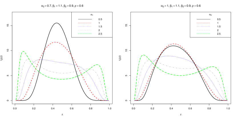
Figure 1: Plot of the PDF $f_{Z}$ with varying parameters $\alpha_{1}$ (left) and $\alpha_{2}$ (right).

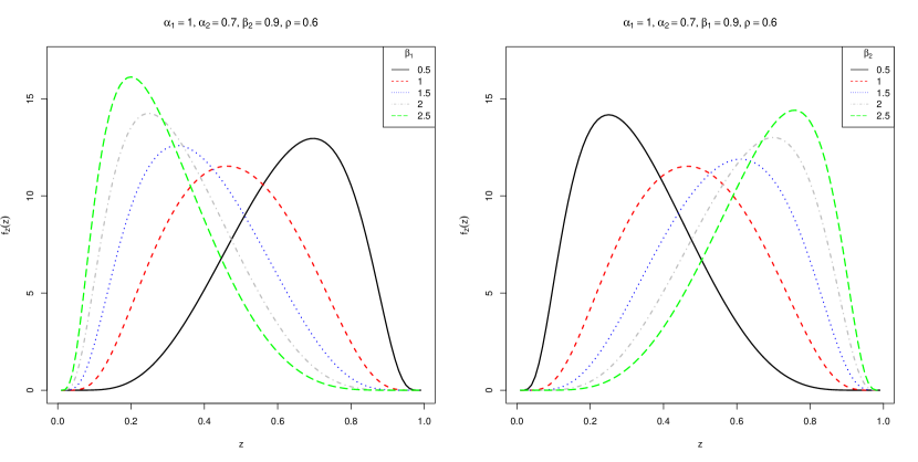
Figure 2: Plot of the PDF $f_{Z}$ with varying parameters $\beta_{1}$ (left) and $\beta_{2}$ (right).

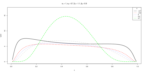
Figure 3: Plot of the PDF $f_{Z}$ with varying parameter $\rho$.

3 Characterization and estimation

In this section, we establish some mathematical results of the UBS distribution. In particular, we define the UBS model as a ratio, present the cumulative distribution function, and calculate the stress-strength probability. We also derive parameter estimators for the UBS model based on the maximum product of spacings method.

3.1 UBS model arising as a ratio

In this section, we establish one of the most important properties of the UBS model. This property characterizes a UBS random variable $Z$ in (2) as a ratio of the form $Y/(X+Y)$, where the random vector $(X,Y)^{\top}$ follows a bivariate Birnbaum-Saunders distribution as discussed in Kundu and Gupta, (2017).

Indeed, let $X,Y$ and $Z$ be continuous and positive random variables such that

$$Z\stackrel{{\scriptstyle d}}{{=}}\dfrac{Y}{X+Y},$$ (6)

being $\stackrel{{\scriptstyle d}}{{=}}$ equality in distribution, and the ratio in (6) has support in the unit interval $(0,1)$. The random variable $Z=Y/(X+Y)$ is known in the literature as type I ratio (Johnson et al., 1995; Bekker et al.,, 2009).

From (6), it is simple to verify that the cumulative distribution function (CDF) of $Z$ is given by

$$F_{Z}(z)=\mathbb{P}\left({X\over Y}\geqslant{s}\right)=1-\int_{0}^{\infty}\mathbb{P}\left(X\leqslant sy|Y=y\right)f_{Y}(y){\rm d}y,\quad s={1\over z}-1.$$ (7)

Hence, the PDF of $Z$ can be expressed as

$$f_{Z}(z)=(s+1)^{2}\int_{0}^{\infty}yf_{X,Y}(sy,y){\rm d}y.$$ (8)

Remark 3.1.

Equation in (8) can also be obtained using the Jacobian method by determining the marginal with respect to $Z$ of the random vector $(Z,U)^{\top}$, where $Z=Y/(X+Y)$ and $U=Y$.

Now, let’s suppose that $(X,Y)^{\top}$ has a bivariate Birnbaum-Saunders distribution with parameter vector $\bm{\theta}_{\rho}=(\alpha_{1},\alpha_{2},\beta_{1},\beta_{2},\rho)^{\top}$, denoted by $(X,Y)^{\top}\sim{\rm BS}(\bm{\theta})$, that is, its joint density is given by

$$f_{X,Y}(x,y)=\phi_{2}(a(x;\alpha_{1},\beta_{1}),a(y;\alpha_{2},\beta_{2});\rho)a^{\prime}(x;\alpha_{1},\beta_{1})a^{\prime}(y;\alpha_{2},\beta_{2}),$$

where $\phi_{2}(u,v;\rho)$ denotes the standard bivariate normal density function;

$$\phi_{2}(u,v;\rho)={1\over 2\pi\sqrt{1-\rho^{2}}}\,\exp\left\{-{1\over 2(1-\rho^{2})}\,(u^{2}+v^{2}-2\rho uv)\right\},\quad(u,v)^{\top}\in\mathbb{R}^{2}$$

and

$$a(t;\alpha,\beta)={1\over\alpha}\left(\sqrt{t\over\beta}-\sqrt{\beta\over t}\right),\quad a^{\prime}(t;\alpha,\beta)={1\over 2\alpha t}\left(\sqrt{t\over\beta}+\sqrt{\beta\over t}\right),\quad t>0.$$ (9)

Hence, the density (8) of $Z$ is written as

$$f_{Z}(z)=(s+1)^{2}\int_{0}^{\infty}y\phi_{2}(a(sy;\alpha_{1},\beta_{1}),a(y;\alpha_{2},\beta_{2});\rho)a^{\prime}(sy,\alpha_{1},\beta_{1})a^{\prime}(y,\alpha_{2},\beta_{2}){\rm d}y.$$ (10)

Since

$$a^{2}(sy;\alpha_{1},\beta_{1})+a^{2}(y;\alpha_{2},\beta_{2})-2\rho a(sy;\alpha_{1},\beta_{1})a(y;\alpha_{2},\beta_{2})$$

$$=\left({u_{\rho}y}+{v_{\rho}\over y}\right)-2\left[{1\over\alpha_{1}^{2}}+{1\over\alpha_{2}^{2}}-{\rho\over\alpha_{1}\alpha_{2}}\left(\sqrt{\beta_{2}s\over\beta_{1}}+\sqrt{\beta_{1}\over\beta_{2}s}\right)\right],$$

with $u_{\rho}$ and $v_{\rho}$ as given in (2), note that the function $\phi_{2}(a(sy;\alpha_{1},\beta_{1}),a(y;\alpha_{2},\beta_{2});\rho)$ in (10) can be expressed as

$$\phi_{2}(a(sy;\alpha_{1},\beta_{1}), \,a(y;\alpha_{2},\beta_{2});\rho)={1\over 2}\,\exp\left\{-{1\over 2(1-\rho^{2})}\left({u_{\rho}y}+{v_{\rho}\over y}\right)\right\}$$

$$\times{1\over\pi\sqrt{1-\rho^{2}}}\,\exp\left\{{1\over 1-\rho^{2}}\left[{1\over\alpha_{1}^{2}}+{1\over\alpha_{2}^{2}}-{\rho\over\alpha_{1}\alpha_{2}}\left(\sqrt{\beta_{2}s\over\beta_{1}}+\sqrt{\beta_{1}\over\beta_{2}s}\right)\right]\right\}.$$ (11)

Furthermore, notice that

$$a^{\prime}(sy;\alpha_{1},\beta_{1})a^{\prime}(y;\alpha_{2},\beta_{2}) ={1\over 4\alpha_{1}\alpha_{2}sy}\left[{1\over y^{2}}\sqrt{\beta_{1}\beta_{2}\over s}+{1\over y}\left(\sqrt{\beta_{2}s\over\beta_{1}}+\sqrt{\beta_{1}\over\beta_{2}s}\right)+\sqrt{s\over\beta_{1}\beta_{2}}\right].$$ (12)

By replacing (3.1) and (12) in formula (10), we have

$$f_{Z}(z) ={1\over\pi\sqrt{1-\rho^{2}}}\,{(s+1)^{2}\over 4\alpha_{1}\alpha_{2}s}\,\exp\left\{{1\over 1-\rho^{2}}\left[{1\over\alpha_{1}^{2}}+{1\over\alpha_{2}^{2}}-{\rho\over\alpha_{1}\alpha_{2}}\left(\sqrt{\beta_{2}s\over\beta_{1}}+\sqrt{\beta_{1}\over\beta_{2}s}\right)\right]\right\}$$

$$\times\left[\sqrt{\beta_{1}\beta_{2}\over s}\,\mathbb{I}_{1}+\left(\sqrt{\beta_{2}s\over\beta_{1}}+\sqrt{\beta_{1}\over\beta_{2}s}\right)\mathbb{I}_{2}+\sqrt{s\over\beta_{1}\beta_{2}}\,\mathbb{I}_{3}\right],$$ (13)

where

$$\mathbb{I}_{1}={1\over 2}\,\int_{0}^{\infty}{1\over y^{2}}\,\exp\left\{-{1\over 2(1-\rho^{2})}\left({u_{\rho}y}+{v_{\rho}\over y}\right)\right\}{\rm d}y=\sqrt{u_{\rho}\over v_{\rho}}\,K_{-1}\left({\sqrt{u_{\rho}v_{\rho}}\over 1-\rho^{2}}\right),$$

$$\mathbb{I}_{2}={1\over 2}\,\int_{0}^{\infty}{1\over y}\,\exp\left\{-{1\over 2(1-\rho^{2})}\left({u_{\rho}y}+{v_{\rho}\over y}\right)\right\}{\rm d}y=K_{0}\left({\sqrt{u_{\rho}v_{\rho}}\over 1-\rho^{2}}\right)$$

and

$$\mathbb{I}_{3}={1\over 2}\,\int_{0}^{\infty}\exp\left\{-{1\over 2(1-\rho^{2})}\left({u_{\rho}y}+{v_{\rho}\over y}\right)\right\}{\rm d}y=\sqrt{v_{\rho}\over u_{\rho}}\,K_{1}\left({\sqrt{{u_{\rho}v_{\rho}}}\over 1-\rho^{2}}\right).$$

In the above, $K_{\lambda}(x)$, $x>0$, denotes the modified Bessel function of the third kind defined in (2).

Finally, by using that the Bessel function is symmetric with respect to the index $\lambda$: $K_{\lambda}(x)=K_{-\lambda}(x)$, and by employing the above formulas of $\mathbb{I}_{1},\mathbb{I}_{2}$ and $\mathbb{I}_{3}$, from (3.1) the PDF of $Z$ can be expressed as in (2).

3.2 The cumulative distribution function

For $(X,Y)^{\top}\sim{\rm BS}(\bm{\theta}_{\rho})$, it holds that $X\sim{\rm BS}(\alpha_{1},\beta_{1})$ and $Y\sim{\rm BS}(\alpha_{2},\beta_{2})$. Furthermore, the conditional CDF of $X$, given $Y=y$, is given by (Kundu et. al,, 2010, Theorem 3.1)

$$\mathbb{P}\left(X\leqslant x|Y=y\right)=\Phi\left\{\dfrac{a(x;\alpha_{1},\beta_{1})-{\rho}a(y;\alpha_{2},\beta_{2})}{\sqrt{1-\rho^{2}}}\right\},$$

where $a(t;\alpha,\beta)$ is as given in (9) and $\Phi$ is the CDF of the standard normal distribution. Hence, from (7) it follows that

$$F_{Z}(z;\bm{\theta}_{\rho}) =1-\int_{0}^{\infty}\mathbb{P}\left(X\leqslant sy|Y=y\right)f_{Y}(y){\rm d}y,\quad s={1\over z}-1,$$

$$=1-\int_{0}^{\infty}\Phi\left\{\dfrac{a(sy;\alpha_{1},\beta_{1})-{\rho}a(y;\alpha_{2},\beta_{2})}{\sqrt{1-\rho^{2}}}\right\}\phi(a(y;\alpha_{2},\beta_{2}))a^{\prime}(y;\alpha_{2},\beta_{2}){\rm d}y,$$

where $\phi$ denotes the PDF of the standard normal distribution. By using the change of variable $w=a(y;\alpha_{2},\beta_{2})$, we write the above expression as

$$1-\int_{-\infty}^{\infty}\Phi\left\{\dfrac{a(sa^{-1}(w;\alpha_{2},\beta_{2});\alpha_{1},\beta_{1})-{\rho}w}{\sqrt{1-\rho^{2}}}\right\}\phi(w){\rm d}w$$

$$={1\over 2}-{1\over 2}\int_{-\infty}^{\infty}{\rm erf}\left\{\dfrac{a(sa^{-1}(w;\alpha_{2},\beta_{2});\alpha_{1},\beta_{1})-{\rho}w}{\sqrt{2(1-\rho^{2})}}\right\}\phi(w){\rm d}w,$$

where we have used the well-known identity $\Phi(x)=({1}/{2})[1+{\mbox{erf}}(x/\sqrt{2})]$. In the above, $a^{-1}(t;\alpha,\beta)$ denotes the inverse function of $a(t;\alpha,\beta)$. As $a^{-1}(t;\alpha,\beta)=(\beta/4)[\alpha t+\sqrt{(\alpha t)^{2}+4}\,]^{2},$ the integral above can be written as

$${1\over 2}-{1\over 2}\int_{-\infty}^{\infty}{\rm erf}\left\{{{\left({\alpha_{2}\over\alpha_{1}}\sqrt{s\beta_{2}\over\beta_{1}}-\rho\right)\over\sqrt{2(1-\rho^{2})}}\,w+{\sqrt{2}(s\beta_{2}-\beta_{1})\over\alpha_{1}\sqrt{s\beta_{1}\beta_{2}(1-\rho^{2})}}\,{1\over\alpha_{2}w+\sqrt{(\alpha_{2}w)^{2}+4}}}\right\}\phi(w){\rm d}w.$$

Therefore, the CDF of the UBS random variable $Z$ is given by (for $s={1/z}-1$ and $0<z<1$)

$$F_{Z}(z;\bm{\theta}_{\rho})={1\over 2}-{1\over 2}\int_{-\infty}^{\infty}{\rm erf}\left\{{{\left({\alpha_{2}\over\alpha_{1}}\sqrt{s\beta_{2}\over\beta_{1}}-\rho\right)\over\sqrt{2(1-\rho^{2})}}\,w+{\sqrt{2}(s\beta_{2}-\beta_{1})\over\alpha_{1}\sqrt{s\beta_{1}\beta_{2}(1-\rho^{2})}}\,{1\over\alpha_{2}w+\sqrt{(\alpha_{2}w)^{2}+4}}}\right\}\phi(w){\rm d}w.$$ (14)

3.3 The stress-strength probability

In what follows we explicitly calculate the stress-strength probability $R\equiv\mathbb{P}(X<Y)$ in the case where $(X,Y)^{\top}\sim{\rm BS}(\bm{\theta}_{\rho})$, that is, $X$ and $Y$ can admit correlation.

Indeed, by (7), we have

$$R=\mathbb{P}\left({X\over Y}<1\right)=1-\mathbb{P}\left({X\over Y}\geqslant 1\right)=1-F_{Z}(z;\bm{\theta}_{\rho})\Big{|}_{z=1/2}.$$

Hence, as $z=1/2$ if and only if $s=1$, by using (14), we get

$$R={1\over 2}+{1\over 2}\int_{-\infty}^{\infty}{\rm erf}\left\{{{\left({\alpha_{2}\over\alpha_{1}}\sqrt{\beta_{2}\over\beta_{1}}-\rho\right)\over\sqrt{2(1-\rho^{2})}}\,w+{\sqrt{2}(\beta_{2}-\beta_{1})\over\alpha_{1}\sqrt{\beta_{1}\beta_{2}(1-\rho^{2})}}\,{1\over\alpha_{2}w+\sqrt{(\alpha_{2}w)^{2}+4}}}\right\}\phi(w){\rm d}w.$$ (15)

In the particular case $\beta_{1}=\beta_{2}$, from (15), the stress-strength probability $R$ is simply written as

$$R={1\over 2}+{1\over 2}\int_{-\infty}^{\infty}{\rm erf}\left\{\dfrac{\left({\alpha_{2}\over\alpha_{1}}-{\rho}\right)}{\sqrt{2(1-\rho^{2})}}\,w\right\}\phi(w){\rm d}w={1\over 2},\quad\forall\rho\in(-1,1),$$

where in the last equality we have used the fact that erf$(x)$ and $\phi$ are odd and even functions, respectively.

To our knowledge, in this setting ($\beta_{1}=\beta_{2}$), identity $R=1/2$ was known only for the special case in which $X$ and $Y$ are independent (that is, $\rho=0$); see, e.g. Saulo et. al, (2019) and Quintino et. al, (2024).

3.4 Maximum product of spacings method

The maximum product of spacings (MPS) method was introduced by Cheng and Amin, (1979, 1983) and Ranneby, (1984) as a different approach to estimating parameters of continuous univariate distributions compared to maximum likelihood estimation. Let $\{Z_{i}:i=1,\ldots,n\}$ be a univariate random sample of size $n$ from the UBS$(\bm{\theta}_{\rho})$ distribution with PDF as in (2), and let $z_{i}$ be the sample observation of $Z_{i}$. Then, the uniform spacings of $\{z_{i}:i=1,\ldots,n\}$ is given by

$$\Delta_{i}(\bm{\theta}_{\rho})=F_{Z}(z_{i:n};\bm{\theta}_{\rho})-F_{Z}(z_{i-1:n};\bm{\theta}_{\rho}),\quad 1,\ldots,n,$$

with $F_{Z}(z_{0:n};\bm{\theta}_{\rho})=0$, $F_{Z}(z_{n+1:n};\bm{\theta}_{\rho})=1$, and $\Delta_{0}(\bm{\theta}_{\rho})+\Delta_{1}(\bm{\theta}_{\rho})+\cdots+\Delta_{n+1}(\bm{\theta}_{\rho})=1$.

The maximum product of spacings estimator, $\widehat{\bm{\theta}}_{\rho}$, is obtained by maximizing the geometric mean of the spacings

$$G(\bm{\theta}_{\rho})=\left(\prod_{i=1}^{n+1}\Delta_{i}(\bm{\theta}_{\rho})\right)^{\frac{1}{n+1}},$$

or, equivalently, maximizing the function

$$H(\bm{\theta}_{\rho})=\frac{1}{1+n}\sum_{i=1}^{n+1}\log(\Delta_{i}(\bm{\theta}_{\rho})).$$

4 Simulation study

In this section, we carry out a Monte Carlo simulation study for evaluating the performance of the above described maximum product of spacings method for the UBS distribution (2). The simulation scenario considers the following setup: 300 Monte Carlo replications, sample size $n\in\{100,200,400,800\}$, and vector of true parameters $(\alpha_{1},\alpha_{2},\beta_{1},\beta_{2})^{\top}=(0.5,0,5,1.0,1.0)^{\top}$, $\rho\in\{0.10,0.25,0.5,0.75\}$.

The performance and recovery of the maximum product of spacings estimators are evaluated by means of relative bias (RB), and root mean square error (RMSE), which are calculated from the Monte Carlo replicates, as

$$\widehat{\textrm{RE}}(\widehat{\gamma}) = \frac{1}{N}\sum_{i=1}^{N}\left|\frac{(\widehat{\gamma}^{(i)}-\gamma)}{\gamma}\right|,\quad\widehat{\mathrm{RMSE}}(\widehat{\gamma})={\sqrt{\frac{1}{N}\sum_{i=1}^{N}(\widehat{\gamma}^{(i)}-\gamma)^{2}}},$$

where $\gamma$ and $\widehat{\gamma}^{(i)}$ are the true parameter value and its $i$-th estimate, and $N$ is the number of Monte Carlo replications. The steps for the Monte Carlo simulation study are as: i. set the values of the parameters of the UBS distribution; ii. generate 300 samples of size $n$ from the chosen model; iii. estimate the model parameters using the maximum product of spacings method method for each sample; and iv. compute the empirical RB and RMSE.

The maximum product of spacings estimation results so obtained are shown in Figures 4 and 5 wherein the empirical bias and RMSE are both plotted. We observe that the results obtained for the UBS distribution are as expected in that as the sample size increases, both RE and RMSE decrease. In terms of the impact of the parameter $\rho$, we observe that both RB and RMSE of $\widehat{\alpha}_{1}$, $\widehat{\alpha}_{2}$, $\widehat{\beta}_{1}$ tend to increase as $\rho$ increases. In the case of $\widehat{\rho}$, we observe the opposite behavior.

Figure 4: Monte Carlo simulation results for the UBS distribution.

Figure 5: Monte Carlo simulation results for the UBS distribution.

5 Application

We now give two applications using real data previously analyzed in the literature. We study the validity of the new model for the data sets and show that UBS distribution presents good fits on both cases.

5.1 Income-consumption data

In order to evaluate the new probabilistic model, a public data set of income and consumption data was used. The data (available at https://www.bancaditalia.it/statistiche/tematiche/indagini-famiglie-imprese/bilanci-famiglie/documentazione/ricerca/ricerca.html?min_anno_pubblicazione=2008&max_anno_pubblicazione=2008, accessed on July 22, 2024) comes from the Bank of Italy’s Survey on Household Income and Wealth from the year 2008.

The income comprises payroll income, pensions and net transfers, net self-employment income, and property income. Consumption consists of expenditures on both durable and non-durable goods. Durable expenditure represents the net balance of purchased and sold goods. Non-durable expenditures include monthly expenses such as rent, food, and other essentials, as well as annual expenses.

We used the data from the survey, available as the data sets RFAM08 (income as $Y$ variable) and RISFAM08 (expenditures as $C$ variable), according to the Survey on Household Income and Wealth 2008 data description file. We removed from the data set lines whose income or consumption was negative or unavailable. Thus, the analyzed data set included information from 7,957 families, after removing 20 lines of the data.

The same data set was also used in Domma and Giordano, (2012) and Lima et al., (2024), however, they used a copula approach to model the data and compared income and consumption through stress-strength measures of the type $\mathbb{P}(X<Y)$. Our framework involves constructing a new variable $U=X/(X+Y)$. In summary, when $X$ and $Y$ represent expenditures and income, respectively, $U<1/2$ indicates that the family ended the year with more expenditures than income. If $U>1/2$, the opposite is true. The case $U=1/2$ means expenditures and income are equal.

Table 1 presents descriptive statistics for $U=X/(X+Y)$. The estimated parameters of UBS model was $\widehat{\bm{\theta}}_{\rho}=(0.275,0.274,1.041,1.331,0.149)$. Figure 6 shows the fit of the UBS distribution to the density and ECDF of the data. The histogram of $U$ shows that with high (81.5%) probability $U>1/2$. That means, in general, the families have income greater than expenditures.

Table 1: Descriptive statistics for income-consumption data.

n	Min.	1st Qu.	Median	Mean	3rd Qu.	Max.	Std. dv.	CS	CK
7,957	0.004	0.514	0.553	0.557	0.608	0.935	0.086	-0.419	3.343

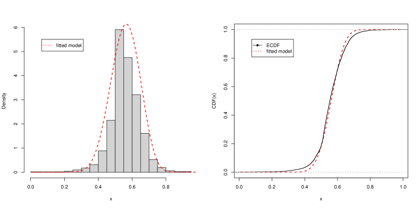
Figure 6: Fitted UBS PDFs (left) and empirical CDF (right) for income-consumption data.

Given that the $U$ data has unit support, we can make a comparison between the utilization of the UBS model and other families of unit distributions, such as Beta and the unit bimodal BS (UBBS) models, as illustrated in Table 2. To obtain the estimation results for Beta and UBBS models in Table 2, we used the package AdequacyModel in the R software. Deciding the better distribution to model the data was oriented by AIC (Akaike information criterion) and BIC (Bayesian information criterion) criteria. In Table 2, these criteria suggest UBS fits the data better than Beta and UBBS models.

Table 2: Estimated parameters for income-consumption data and model selection with AIC and BIC.

Model	$\hat{\bm{\theta}}$	$ll_{max}$	AIC	BIC
UBS	(0.275, 0.274, 1.041, 1.331, 0.149)	-7,062.74	-14,135.49	-14,170.40
Beta	(7.492, 6.390)	-6,877.40	-13,750.79	-13,736.83
UBBS	(1.726, 0.589, 9.545)	-3,614.60	-7,223.20	-7,202.25

5.2 Body mass data

Biomedical measurements of 202 athletes from different sports are presented in the Australian Institute of Sport (AIS) data set. Martínez-Flórez et al., (2024) proposed the UBBS model and showed its fit on the distribution of the percentage of the body fat complement of the athletes. In this subsection, we show that the new UBS model is an alternative distribution to fit that data. The data were imported directly through the software R by the command:

library(sn)
data(ais)
u=1-(ais$Bfat/100)

Descriptive statistics for $\mathbf{u}$ (the athlete’s body mass in the data set) are presented in Table 3. As the data set has unit support, the UBS distribution is a candidate to model such data. Figure 7 shows the fit of UBS to the data. Maximum likelihood estimates and maximum product of spacings estimates can be compared graphically.

Table 3: Descriptive statistics of athlete’s body mass in the data set.

Min.	1st Qu.	Median	Mean	3rd Qu.	Max.	Std. dv.	CS	CK
0,645	0,819	0,884	0,865	0,915	0,944	0,062	-0,754	-0,201

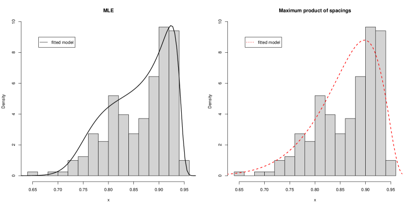
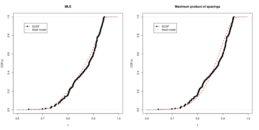
Figure 7: Plots for the athlete’s body mass. On top, histogram and fitted UBS PDFs (ML estimates on left and Maximum product of spacings estimates on right); on bottom, Empirical CDF and fitted UBS CDF.

In Table 4, when comparing the UBS model (with parameter estimates via product of spacings) with the Beta and UBBS models using information criteria, the BIC indicates the new model is better to fit the athlete’s body mass data. However, when considering the AIC, the UBBS model should be chosen.

Table 4: Estimated parameters for the athlete’s body mass data and model selection with AIC and BIC.

Model	$\hat{\bm{\theta}}$	AIC	BIC
UBS	(0.149, 0.626, 0.296, 2.003, 0.586)	-613.10	-629.64
Beta	(0.865, 0.173)	-585.32	-578.70
UBBS	(0.284, 0.137, -1.353)	-626.64	-616.72

6 Concluding remarks

In this paper, we have introduced a new unit distribution. Its generation as a ratio of possibly dependent Birnbaum-Saunders random variables has been discussed in detail. As a more theoretical part, we have derived the cumulative distribution function and the stress-strength probability. As practical issues, we presented maximum product of spacings estimators and applications to income-consumption and body mass data sets.

The research could be continued in several directions. One could investigate the moments and the moment generating function and try to express shape characteristics like skewness and kurtosis. The analysis of the entropy of the distribution could also be of interest. Instead of using the ratio $Y/(X+Y)$ one could explore other construction principles like those mentioned in the introduction to obtain a unit distribution. Finally, one could use a bivariate distribution other than the Birnbaum-Saunders to construct a unit distribution.

Acknowledgements

This study was financed in part by the Coordenação de Aperfeiçoamento de Pessoal de Nível Superior - Brasil (CAPES) - Finance Code 001.

Disclosure statement

There are no conflicts of interest to disclose.

References

• Abramowitz and Stegun, (1972) M. Abramowitz and I. A. Stegun, (eds.): Handbook of Mathematical Functions, 9th edn. Dover, New York (1972).
• Afifi et al., (2022) A. Z. Afifi, M. Nassar, D. Kumar, and G.M. Cordeiro, A New Unit Distribution: Properties, Inference, and Applications, Electronic Journal of Applied Statistical Analysis (2022), 15(02), pp. 460–484,
• Bekker et al., (2009) A. Bekker, J. Roux, and T. Pham-Gia, The type I distribution of the ratio of independent “Weibullized” generalized beta-prime variables, Statistical Papers (2009), 50, pp. 323–338.
• (4) Z. W. Birnbaum and S. C. Saunders, A new family of life distributions, Journal of Applied Probability (1969), 6(2), pp. 319-327.
• (5) Z. W. Birnbaum and S. C. Saunders, Estimation for a family of life distributions with applications to fatigue, Journal of Applied Probability (1969), 6(2), pp. 328–347.
• Bourguignon et al., (2024) M. Bourguignon, H. Saulo, and D. Gallardo. Parametric quantile beta regression model, International Statistical Review (2024), 92, pp. 106–129.
• Cheng and Amin, (1979) R. C. H. Cheng and N. A. K. Amin, Maximum product-of-spacings estimation with applications to the lognormal distribution, Technical Report, Department of Mathematics, University of Wales (1979).
• Cheng and Amin, (1983) R. C. H. Cheng and N. A. K. Amin, Estimating parameters in continuous univariate distributions with a shifted origin, Journal of the Royal Statistical Society. Series B (1983), 3, pp. 394–403.
• Condino and Domma, (2023) F. Condino and F. Domma, Unit Distributions: A General Framework, Some Special Cases, and the Regression Unit-Dagum Models, Mathematics (2023), 11, 2888.
• Cortés et al., (2018) M. A. Cortés, D. Elal-Olivero, and J.,F. Olivares-Pacheco, A New Class of Distributions Generated by the Extended Bimodal-Normal Distribution, Journal of Probability and Statistics, (2018), 1-10.
• Desmond, (1985) A. Desmond, Stochastic models of failure in random environments, Canadian Journal of Statistics (1985), 13(3), pp. 171–183.
• Domma and Giordano, (2012) F. Domma and S. Giordano, A stress–strength model with dependent variables to measure household financial fragility, Statistical Methods & Applications (2012), 21, pp. 375–389.
• Johnson et al. (1995) N. L. Johnson, S. Kotz, and N. Balakrishnan, Continuous Univariate Distributions - Vol. 2. John Wiley & Sons, New York (1995).
• Jørgensen, (1982) B. Jørgensen, Statistical Properties of the Generalized Inverse Gaussian Distribution, Lecture Notes in Statistics, vol. 9. Springer, New York (1982).
• Kundu and Gupta, (2017) D. Kundu and R. C. Gupta, On Bivariate Birnbaum-Saunders Distribution, American Journal of Mathematical and Management Sciences (2017), 36(1), pp. 21–33.
• Kundu et. al, (2010) D. Kundu, N. Balakrishnan and A. Jamalizadeh, Bivariate Birnbaum-Saunders distribution and associated inference, Journal of Multivariate Analysis (2010), 101, pp. 113–125.
• Lima et al., (2024) R. Lima, F. Quintino, T. da Fonseca, L. Ozelim, P. Rathie and H. Saulo, Assessing the Impact of Copula Selection on Reliability Measures of Type $P(X<Y)$ with Generalized Extreme Value Marginals, Modelling (2024), 5(1), pp. 180-200.
• Martínez-Flórez et al., (2024) G. Martínez-Flórez, N. Olmos and O. Venegas, Unit-bimodal Birnbaum-Saunders distribution with applications, Communications in Statistics-Simulation and Computation (2024), 53(5), pp. 2173-2192.
• Teimouri et. al, (2013) M. Teimouri, S. M. Hosseini and S. Nadarajah, Ratios of Birnbaum-Saunders Random Variables, Quality Technology & Quantitative Management (2013), 10, pp. 457–481.
• Quintino et. al, (2024) F. S. Quintino, L. C. d. S. M. Ozelim, T. A. d. Fonseca and P. N. Rathie, Stress-Strength Reliability of the Type $\mathbb{P}(X<Y)$ for Birnbaum-Saunders Components: A General Result, Simulations and Real Data Set Applications, Modelling (2024), 5, pp. 223–237.
• Ranneby, (1984) B. Ranneby, The maximum spacing method. An estimation method related to the maximum likelihood method, Scandinavian Journal of Statistics (1984), 11, pp. 93–112.
• Saulo et. al, (2019) H. Saulo, J. Leão, R. Vila, V. Leiva and V. Tomazella, On mean-based bivariate Birnbaum-Saunders distributions: Properties, inference and application, Communications in Statistics - Theory and Methods (2019), 49(24), pp. 6032–6056.
• (23) R. Vila, L. Alfaia, A.F.B. Menezes, M.N. Çankaya, and M. Bourguignon, A Model for Bimodal Rates and Proportions, Journal of Applied Statistics (2024), 51(4), pp. 664–681.
• (24) R. Vila, N. Balakrishnan, and Bourguignon, M, On the distribution of a random variable involved in an independent ratio, Communications in Statistics-Theory and Methods (2024), https://doi.org/10.1080/03610926.2024.2340608.
• (25) R. Vila, N. Balakrishnan, H. Saulo, and P. Zörnig, Unit-log-symmetric models: characterization, statistical properties and their applications to analyzing an internet access data, Quality and Quantity (2024), https://doi.org/10.1007/s11135-024-01879-w.
• Zörnig, (2023) P. Zörnig, A new type of skew uniform distribution, Asian Journal of Statistical Sciences (2023), 3, pp. 27–39.