revtex4-2Repair the float \theoremstyledefinition
Full classification of Pauli Lie algebras
Abstract
Lie groups, and therefore Lie algebras, are fundamental structures in quantum physics that determine the space of possible trajectories of evolving systems. However, classification and characterization methods for these structures are often impractical for larger systems. In this work, we provide a comprehensive classification of Lie algebras generated by an arbitrary set of Pauli operators, from which an efficient method to characterize them follows. By mapping the problem to a graph setting, we identify a reduced set of equivalence classes: the free-fermionic Lie algebra, the set of all anti-symmetric Paulis on qubits, the Lie algebra of symplectic Paulis on qubits, and the space of all Pauli operators on qubits, as well as controlled versions thereof. Moreover, out of these, we distinguish 6 Clifford inequivalent cases and find a simple set of canonical operators for each, which allow us to give a physical interpretation of the dynamics of each class. Our findings reveal a no-go result for the existence of small Lie algebras beyond the free-fermionic case in the Pauli setting and offer efficiently computable criteria for universality and extendibility of gate sets. These results bear significant impact in ideas in a number of fields like quantum control, quantum machine learning, or classical simulation of quantum circuits.
I Introduction
Lie groups emerge as a fundamental mathematical structure in quantum physics due to their intrinsic connection to the Schrödinger equation. The set of possible trajectories of an evolving quantum system is confined to the Lie group associated with the generators of the dynamics. Consequently, the study and classification of continuous symmetries and dynamics in quantum physics can be framed in terms of the analysis of such objects. Often, this analysis can be simplified by instead examining the tangent spaces of these Lie groups, namely Lie algebras, where the commutation relations of their elements encode the essential information about the evolution.
This connection has been studied extensively in several fields within quantum information theory and quantum computation. In quantum control theory, universality and controllability questions are entirely ones of reachability, and hence Lie-algebraic in nature, making the study of these structures crucial for the design of universal quantum gate-sets and simulators [1, 2, 3, 4]. Lie algebras have also been shown to play a crucial role in understanding and designing variational quantum algorithms [5, 6] and quantum machine learning methods [7], where in certain scenarios have been directly linked to phenomena like barren plateaus and overparametrization [8]. Additionally, approaches such as geometric quantum machine learning [9, 10, 11] also rely on Lie algebraic notions in order to simplify training by embedding problem specific symmetries into the circuits. Finally, ideas in quantum circuit complexity, like measures based on operators spread, are also strictly related to the Lie algebra spanned by the circuit generators [12, 13, 14, 15] , and hence also the classical simulability of some families of quantum circuits [16, 17, 18, 19].
Classification and characterization of Lie algebras are thus crucial for the further development of these fields. In a general setting however, this task often becomes intractable. Consequently, progress in this regard has been restricted to specific instances, where it is possible to rely on certain algebraic structural properties, like simplicity [20], or to construct an explicit basis of the Lie algebra, which is only feasible under strict assumptions on the generators [21, 22, 23, 24, 25, 26, 27], like locality or periodicity.
This work adds to this literature by giving a comprehensive classification of all Pauli Lie algebras, these being all Lie algebras generated by any set of Pauli operators, and also providing an efficient method to determine the Lie algebra of an arbitrary set of Pauli generators. Pauli operators are particularly interesting because they form a basis for all Hermitian operators. As such, they appear as natural generators in many popular gate sets in the context of digital quantum computing and become relevant in a plethora of tasks, like whenever one considers Hamiltonian simulation techniques based on product formulas [28, 29, 30, 31, 17]. Moreover, their particular commutation structure resembles that of Majorana operators in fermionic systems, thus making them directly useful for their study.
Due to these commutation and anti-commutation rules of Pauli operators, which we will leverage to simplify the problem, our work bears big resemblance to studies on (quasi-)Clifford Lie algebras in the mathematics literature [32, 33, 34]. While these studies focus on the mathematical structure of the Lie algebra, we aim to characterize these sets in a way that allows us to make further remarks about the embedding Hilbert space and the physics of their evolution. The key component in our analysis will be to map the classification problem to a graph reduction problem. This approach will be similar in spirit to previous works like Bouchet’s on graph equivalence under local complementations [35] – that has important implications on assessing whether two graph states [36] are equivalent under sequences of local Clifford conjugations [37, 36] – or others considering the vertex minor problem, where vertex deletion is also considered [38, 39]. In our case, we will find a set of universal equivalence classes for graphs under conditioned local complementations. This will allow us to identify the existence of 6 total Clifford inequivalent Lie algebras. Having that any given collection of initial operators can be mapped through Clifford operations to one of these six simpler sets, we will then derive their Lie algebra type and provide a physical interpretation of their structure along with their relationships.
This reveals that the biggest polynomially-sized Pauli Lie algebra is that of free-fermions together with their parity operator. All other non-free-fermionic cases correspond to the full set of Paulis on -qubits as well as an embedding thereof in an -qubit Hilbert space, the space of all anti-symmetric Pauli operators, and the space of symplectic Pauli operators, each exhibiting a dimension growing exponentially with system size. Beyond these cases, only controlled versions of these dynamics exist.
The remainder of this work is structured as follows. In Section II we define the structures we are interested in, as well as the operations required for the reduction. In Section III we introduce the main theorems of this work regarding graph reductions and their mapping to Lie algebra types. We add the distinction between Clifford inequivalent Lie algebras in Section IV. With all Lie algebra types layed down, we discuss their physical interpretation in Section V. In Section VI, we make a final remark regarding disconnected graphs for completeness, and we finalize in Section VII with a brief discussion of the implications of our results. We prove most of the statements in this work in the Supplemental Material.
II Definitions and setting
The statement of our results will require some preparation. Let us first define our main object of interest.
Definition 1 (Pauli Lie algebra)
We define a Pauli Lie algebra as the Lie algebra whose elements are Pauli strings of some -qubit system, which is closed under the Lie bracket, (), given by the imaginary commutator of its elements, . Then, a set of Paulis is a generating set of if they span all elements in through Lie algebraic operations. Then we write . A generating set is minimal, if removing any would change the size of the Lie-algebra.
Pauli Lie algebras have a very appealing structure since Pauli strings have simple commutation relations, namely given any two Paulis they either commute or anti-commute and the resulting operator is again a Pauli up to a constant. For two non-commuting Paulis , it holds that
| (1) |
where is itself another Pauli. Moreover, Pauli operators are particularly interesting since they form an orthonormal basis for the space of operators. A natural question to ask then, is whether one can characterize all Pauli Lie algebras generated by some arbitrary set . Like we already mentioned in the introduction, one common approach to address this, has been to explicitly construct a basis for the Lie algebra by repeatedly taking nested commutators of the generating elements [21, 40]. However, since the size of the Lie algebra could be exponential, this method is in many cases not scalable.
Here, we will propose a new strategy that overcomes this by mapping the problem to a graph problem. Exploiting some of the already mentioned properties of Pauli operators, we will be able to characterize Pauli Lie algebras for an arbitrary set of generators. This connection is expected to be fruitful, in a way that is reminiscent of the way graph states [36] constitute a theoretical laboratory to study questions in entanglement theory.
Since the basis of the Lie algebra is generated through the commutator of its elements, and the commutator of two Paulis is either 0 or their product, all the information of the basis elements is already encoded exclusively in the commutation relations of the elements in , so long as the generators in are Lie algebraically independent, that is, no generator can be computed through commutators of others. This is satisfied if the generators form a minimal set. For now we assume that we are given a minimal set of generators, but then we lift this assumption in Section IV.1. This allows us to study the Lie algebra by the anti-commutation relations of the generators .
Definition 2 (Anti-commutation graph)
Given a set of Pauli operators , we call its anti-commutation graph the graph , where every vertex corresponds to some , and two vertices are connected by an edge if their corresponding Paulis anti-commute, i.e.,
| (2) |
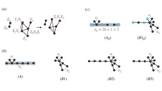
In general, this can be any possible graph for sufficently many qubits. In Figure 1(a, left), we show the anti-commutation graph for the Lie algebraically independent set .
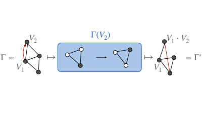
Our goal will be to find a set of universal equivalence classes for graphs, that allows us to determine the Lie algebra associated to any given graph. To that end, we will define graph operations that leave the underlying Lie algebra invariant, and restate our problem as a graph reducibility problem under such operations. The operation in question will be a conditional local complementation. Namely, given two vertices , we will complement edges conditioned on sharing an edge with or not. On the level of the Paulis, this will correspond to replacing, in the generating set, , i.e., replacing a generator by its commutator with another generator.
Definition 3 (Contraction)
Given two non-commuting generators , a contraction of onto maps and . This leaves the Lie algebra invariant .
It is easy to see that indeed this operation does not change the Lie algebra because of the fact that . As such, the set generated from nested commutators of contains all those generated by . Like we said however, for the anti-commutation graph , this transformation will result in a new graph with modified connectivity. In more concrete terms, for the associated vertices , corresponding to , a contraction of onto amounts to a complementation of the edges . In terms of the adjacency matrix of the graph , this is performed by adding the the columns and rows corresponding to vertex onto the columns and rows corresponding to vertex in .
An example of such a contraction is shown in Figure 1(a, right). In the following section we will describe universal equivalence classes under these contractions and how can that help us determining the Lie algebra in the most general case.
III Canonical graph types and Lie algebras
We establish that using graph contractions, every anti-commutation graph is reducible to one of a few canonical types.
Theorem 1 (Canonical graphs)
For any given connected graph with at least two vertices, there exists a sequence of contractions which result in one of four graphs:
-
(A)
A line graph with with vertices as well as single vertices connected to the second to last vertex.
-
(B)
A star graph with legs of length of at most and where the number of legs of length 1 and 2 are , with and , respectively. Additionally, they can present the following:
-
(1)
no legs of length or ,
-
(2)
one leg of length and no leg of length ,
-
(3)
one leg of length and no leg of length .
-
(1)
The canonical types are shown in Figure 1(b).
(Sketch) The full proof is in Appendix B. The statement is proven by induction. The procedure works by selecting some initial vertex at random and iteratively adding new vertices. We show that if the starting graph is one of the considered here, if one adds a new vertex with some arbitrary connectivity to it, there is always a sequence of contractions that transforms the new graph to one of these types. One important remark is that for any given initial graph , the set of contractions that map it to one of these canonical representatives can be found efficiently. Since the proof works inductively in the number of vertices, applying a known set of transformations, one can find an algorithm that is efficient in the number of vertices of that finds the corresponding class. We leave the explicit algorithm for future work.
With this, one can then classify the Lie algebras generated by a minimal set of Paulis by only looking at their graph and the canonical representative it maps to. This brings us to the main result providing the classification of the Lie algebra types.
Theorem 2 (Classification of Pauli Lie algebra types)
Given a set of Lie algebraically independent Paulis , with connected anti-commutation graph , then its Pauli Lie algebra corresponds to one of the following cases.
-
•
when maps to some in class A.
-
•
when maps to some in B1.
-
•
when maps to some in B2.
-
•
when maps to some in B3.
(Sketch) The full proof can be found in the appendices. In Appendix E we prove the terms .The main idea will be to show that several legs of length 1 act as a control register, thus splitting into two equal, smaller Lie algebras. The rest of the statement is proven by construction in Appendix F. The key will be to come up with a good set of canonical Pauli operators, for which it is easy to show, and since the Lie algebra type is uniquely determined by the graph, argue for the general case. For graphs in class A, we will explicitly construct a set of free-fermionic majorana operators and show that this is indeed equivalent to For graphs in B1 and B2, we will show that some set of canonical generators obey the properties defining respectively, and thus they span a sub-algebra of those. On the other hand, we will come up with a set of rules to compute non-zero commutators on these graphs, and show that every element in can actually be written as such a commutator, thus showing equality with the Pauli Lie algebra spanned by our set. Finally, for graphs in B3 we will just show that every Pauli can be computed through nested commutators of our generators. Crucially, the classification of the Lie algebras does not depend directly on the number of qubits of the system. For our purposes, however, besides the structure of the algebra, it will also be relevant to see how a Lie algebra acts within the physical Hilbert space, which we will address in the following sections.
IV Clifford equivalence of Pauli Lie algebras
So far we have discussed the anti-commutation relations for a minimal set of Pauli generators. However, Paulis can also have algebraic dependencies, meaning that even if no generator can be written as a non-zero commutator of others, we could have some generators being a product of others. This is relevant for our next theorem
Lemma 1
(Clifford equivalence lemma) Two Pauli Lie algebras are Clifford equivalent if they can be mapped to the same anti-commutation graph , where the generators share the same algebraic dependencies.
This follows from the general properties of Cliffords [41]. In general it also holds that if two Lie algebras are not Clifford equivalent, then they are also not unitarily equivalent since no unitary can change commutation relations or algebraic dependencies. As such, we would like to determine all possible algebraic dependencies within the Pauli Lie algebra of some minimal generating set. We can establish the following theorem.
Theorem 3 (Limits to algebraic dependencies)
Every minimal generator Pauli Lie algebra has at most one algebraic dependence. Algebraic dependencies can only occur for graphs of type A and B3. These can be mapped by contraction to only one possible case each which are shown in Figure 1 (c). As such, there is a total of Clifford inequivalent families of Pauli Lie algebras.
(Sketch) The full proof can be found in Appendix D, but we state the main idea here. For this it is enough to check algebraic dependencies within the generating set of the graphs in Theorem 1, as contractions preserve algebraic and Lie algebraic dependencies. Given these specific anti-commutation relations, the sets of vertices that can be algebraically dependent are limited to subsets involving legs of odd length, where the ’s appear in an alternating fashion in . Moreover, we will show that since algebraic dependence between legs of length 1 also implies Lie algebraic dependence, the only cases left are the ones stated in the theorem.
IV.1 Finding the minimal set of generators
The scenario described above assumes that we have a minimal set of generators. In general, this might not be the case however. If the set is not minimal, then a generator can be removed. The strategy is to still perform all the graph transformations to get to a canonical form which leaves the Lie algebra invariant even it is not the minimal set. By Gaussian elimination one can identify algebraic dependencies between generators, which is a necessary condition for Lie algebraic dependence. For the canonical types, algebraic dependencies can only occur between legs of length 1 and on a long leg of odd length in an alternating structure (as in theorem 3). Since the latter is an allowed dependence, a redundant generator will necessarily result in an algebraic relation involving only legs of length . In this case one of the involved vertices can be safely removed without changing the Lie algebra. This process can be (efficiently) repeated until all Lie-algebraic dependencies are removed.
V General description of all Pauli Lie-algebras
In this section, we will give an intuition behind our classification result. First of all, we show in Appendix E that the direct sums in Theorem 2, translate to an actual direct sum within the physical Hilbert space. Namely, given several legs of length , using Cliffords, we can always map the Lie algebra to be of the form
| (3) |
where labels each block in the direct sum, and corresponds to operators in the Lie algebra where all additional legs of length 1 are removed (). Then, from Equation 3 it is clear that these additional legs of length 1 always introduce a new qubit register acting as a control on the dynamics given by .
With this, we can now move on to considering each of the 6 types from Theorem 3 without additional legs of length 1 (and hence qubit registers). From now on, we will refer to as being the minimal number of qubits required to span their dynamics (hence the total number of minimal qubits will actually correspond to ). We will show in Appendix E that this number , like for the case of controls, can easily be derived from the number of vertices of the graph.
For type , the number of qubits corresponds to . Then the Lie algebra corresponds to or depending on the parity of . In both cases, this corresponds to the free-fermionic Lie algebra, where can be seen as generated by all Majorana operators on modes, i.e., both first and second order operators
| (4) |
while can be thought as being generated just by second order operators
| (5) |
For the algebraic dependent case , the generating set in terms of Majorana operators becomes which corresponds to the set of free-fermionic operations on modes, together with their parity operator have a Lie algebra of type
| (6) | ||||
which is then the largest connected Pauli Lie algebra on qubits of polynomial size. In this case, these new terms arising from having the parity operator as a generator lead to dynamics allowing more independent dynamics between both fermionic parity operators, compared to the case. A Lie algebra of this class is discussed in Ref. [24], as arising from some many-body systems like the Kitaev honeycomb model in two dimensions [42].
Moving on to the exponentially big Lie algebras, the number of qubits can be given as a function of the number of legs of length 2. Then, for B1 the Lie algebra corresponds to , which describes the space of all Paulis on qubits (here ) satisfying the symplectic condition, i.e., given some
| (7) |
This Lie algebra has recently been motivated, and its properties have been further studied in Ref. [43]. The Lie algebra given by B2 instead, corresponds to , i.e., the span of all purely imaginary Paulis () in the same Pauli basis on qubits (here ). Then, for , we have
| (8) |
This subalgebra has been previously studied in relation to Haar random circuits and benchmarking tasks, when one needs to restrict to some subspace of the full unitary group, for instance, when working with certain fault-tolerant error correcting codes [44, 45]. Moreover, both and can arise when considering operators in commonly studied 1-dimensional spin models, such as the Kitaev chain or the -model under certain interaction fields [21]. For the last two cases, for we have , the full Lie algebra of trace-less Hermitian matrices on qubits ()
| (9) |
On the other hand, is equivalent to all Hermitian matrices on qubits (), which can be understood as the embedding of a complex vector space into a real one () [46]. The Paulis take the form . Then
| (10) | |||
Note that all the definitions given above for the exponentially big Lie algebras are given in a Clifford invariant form, i.e., under Clifford transformations we just have preserving the (anti-) symmetric property.
VI Disconnected Pauli Lie-algebras
Hitherto the discussion centered around connected anti-commutation graphs. However, one could also have a generating set with a disconnected anti-commutation graph. In that case, in general, different connected components are Lie algebraically independent and, therefore, their Lie-algebras are direct sums (in terms of their representations) of the Lie algebras of the subgraphs
| (11) |
where is the number of connected subgraphs and is the Lie algebra of a connected subgraph. If there is no algebraic dependence between their generators, then they are Clifford equivalent to Lie algebras acting on the tensor product of their Hilbert spaces. In general, generators of different sub Lie-algebras can still have an algebraic dependence between them, creating unitarily inequivalent Lie-algebras. For this to occur, we need to consider the non-trivial center of a Lie algebra
| (12) |
where is the algebra generated by the elements of . To have an algebraic dependence, two sub Lie algebras need to share their non-trivial center (). The non-trivial center of the whole Lie algebra we call . The non-trivial center arises from two sources:
-
•
The product of two Paulis corresponding to vertices of legs of length 1.
-
•
If the graph has a non control symmetry. This is the case if does have an algebraic dependence but does not, i.e., the graph is of a structure admissible to or , but no algebraic dependence.
As such, the number of independent generators of the algebra of the center is given by
| (13) |
where describes the presence of the additional symmetry. With this the total number of generators in the non-trivial center is
| (14) |
where the difference between both quantities and comes from algebraic dependencies between disconnected components. In that case, it suffices to describe the algebraic relation between a chosen set of generators of the respective centers of and the generators of (). The full set of dependencies can therefore be described by a matrix where , corresponding to a generator of a non-trivial center of a sub Lie algebra, is given by . For connected anti-commutation graphs, there are only polynomially many (in the number of vertices) Clifford inequivalent Lie algebras, corresponding to the canonical types. If we allow for disconnected graphs, due to the freedom to reuse controls and potential symmetries in the case of A and B3, the number of Clifford inequivalent Pauli Lie algebras becomes exponentially big in general.
VII Discussion and outlook
In this work, we have presented a full classification of Pauli Lie algebras, as well as a sketch on how to algorithmically compute them. Having found a universal set of equivalence classes for graphs under conditioned complementation, our results ultimately serve as a rigorous proof showing that every Pauli Lie algebra is, up to direct sums, either free-fermionic or exponentially large, including all types , and . Additionally, we find an interpretation for direct sums in terms of the physical Hilbert space, as either tensor products, or as actual direct sums coming from gates acting as controlled operations. These considerations regarding the Hilbert space also reveal the existence of 6 Clifford inequivalent Lie algebras. In particular, we show that for and , one can always find a Clifford mapping any generating set to another. In contrast, for the free-fermionic and , one can have two Clifford inequivalent versions. In the former case they are related through inclusion of the fermionic parity operator, and in the latter, by the embedding of the Lie algebra into a larger Hilbert space.
We believe our results can be taken and interpreted in basically two ways. On the one hand, one can see them as a no-go result for the existence of sub-exponential Pauli Lie algebras other than the mentioned free-fermionic ones. Free fermions been used as toy models and studied in a wide range of fields, including quantum machine learning and variational methods [47, 48], as well as simulation techniques of quantum systems [49, 50, 51], and hence their behavior is well understood. This is relevant as our results limit any further avenues for methods within these fields relying on polynomially sized Pauli Lie algebras, like is the case for , geometric QML and others.
While our result only holds for Pauli generators, it would be interesting to study whether these restrictions hold for more general operators, e.g., when considering linear combinations of Paulis. In recent work, for instance, similar graph tools have been used to identify free-fermionic Hamiltonians given by arbitrary sums of Paulis [24, 25]. It would be relevant to find out if this could be extended to identify all possible Lie algebras in a similar way as we do here.
On a more positive note, our work can be viewed as a new framework for efficiently computing Lie algebraic criteria for universality and controllability of Pauli gate sets. Our techniques not only provide an answer to this, but also elucidate a clear way to extend some given operator pool to transition from one Lie algebra to another, offering valuable insights into the structure and capabilities of these gate sets. We believe that this can be used to study properties of quantum circuits when doped with some additional set of gates outside their Lie algebra.
To summarize, efficient and generic tools for classifying and characterizing Lie algebras are crucial in quantum information theory. This work then provides a comprehensive classification of Pauli Lie algebras without any additional assumption on the generators. In doing so, we highlight the limitations that some quantum machine learning and simulation methods might face, while also offering a new tool to address questions regarding reachability and equivalence of gate sets generated by Pauli operators. We believe this work can help in assessing questions that might have remained elusive to date, as well as motivate new algebraic methods in order to deal with other families of operators.
Acknowledgments
We thank Lorenzo Leone, Greg White and Hakop Pashayan for useful discussions. This work has been supported by the BMBF (FermiQP, MuniQCAtoms, DAQC), the Munich Quantum Valley (K-8), the Quantum Flagship (PasQuans2, Millenion), the DFG (CRC 183), the Einstein Research Unit, Berlin Quantum, and the ERC (DebuQC).
References
- Koch et al. [2022] C. P. Koch, U. Boscain, T. Calarco, G. Dirr, S. Filipp, S. J. Glaser, R. Kosloff, S. Montangero, T. Schulte-Herbrüggen, D. Sugny, and F. K. Wilhelm, EPJ Quant. Tech. 9, 19 (2022).
- Dirr and Helmke [2008] G. Dirr and U. Helmke, GAMM Mitt. 31, 59 (2008).
- DiVincenzo [1995] D. P. DiVincenzo, Phys. Rev. A 51, 1015 (1995).
- Sleator and Weinfurter [1995] T. Sleator and H. Weinfurter, Phys. Rev. Lett. 74, 4087 (1995).
- Cerezo et al. [2021] M. Cerezo, A. Arrasmith, R. Babbush, S. C. Benjamin, S. Endo, K. Fujii, J. R. McClean, K. Mitarai, X. Yuan, L. Cincio, and P. J. Coles, Nature Rev. Phys. 3, 625 (2021).
- McClean et al. [2016] J. R. McClean, J. Romero, R. Babbush, and A. Aspuru-Guzik, New J. Phys. 18, 023023 (2016).
- Biamonte et al. [2017] J. Biamonte, P. Wittek, N. Pancotti, P. Rebentrost, N. Wiebe, and S. Lloyd, Nature 549, 195 (2017).
- McClean et al. [2018] J. R. McClean, S. Boixo, V. N. Smelyanskiy, R. Babbush, and H. Neven, Nature Comm. 9, 4812 (2018).
- Nguyen et al. [2024] Q. T. Nguyen, L. Schatzki, P. Braccia, M. Ragone, P. J. Coles, F. Sauvage, M. Larocca, and M. Cerezo, PRX Quantum 5, 020328 (2024).
- Meyer et al. [2023] J. J. Meyer, M. Mularski, E. Gil-Fuster, A. A. Mele, F. Arzani, A. Wilms, and J. Eisert, PRX Quantum 4, 010328 (2023).
- Anschuetz et al. [2023] E. R. Anschuetz, A. Bauer, B. T. Kiani, and S. Lloyd, Quantum 7, 1189 (2023).
- Nielsen et al. [2006] M. A. Nielsen, M. R. Dowling, M. Gu, and A. M. Doherty, Science 311, 1133 (2006).
- Haferkamp et al. [2022] J. Haferkamp, P. Faist, B. T. K. N, J. Eisert, and N. Y. Halpern, Nature Phys. 18, 528 (2022).
- Brandão et al. [2021] F. G. Brandão, W. Chemissany, N. Hunter-Jones, R. Kueng, and J. Preskill, PRX Quantum 2, 030316 (2021).
- Patramanis and Sybesma [2024] D. Patramanis and W. Sybesma, SciPost Phys. Core 7, 037 (2024).
- Goh et al. [2023a] M. L. Goh, M. Larocca, L. Cincio, M. Cerezo, and F. Sauvage, (2023a), arXiv:2308.01432 .
- Begušić et al. [2023] T. Begušić, K. Hejazi, and G. K.-L. Chan, (2023), arXiv:2306.04797 .
- Zimborás et al. [2014] Z. Zimborás, R. Zeier, M. Keyl, and T. Schulte-Herbrueggen, EPJ Quant. Tech. 1, 11 (2014).
- Gu et al. [2021] S. Gu, R. D. Somma, and B. Şahinoğlu, Quantum 5, 577 (2021).
- Cartan [1914] E. Cartan, Ann. Sc. l’École Normale Sup. 3e série, 31, 263 (1914).
- Wiersema et al. [2023] R. Wiersema, E. Kökcü, A. F. Kemper, and B. N. Bakalov, (2023), arXiv:2309.05690 .
- Pozzoli et al. [2022] E. Pozzoli, M. Leibscher, M. Sigalotti, U. Boscain, and C. P. Koch, J. Phys. A 55, 215301 (2022).
- Oszmaniec and Zimborás [2017] M. Oszmaniec and Z. Zimborás, Phys. Rev. Lett. 119, 220502 (2017).
- Chapman and Flammia [2020] A. Chapman and S. T. Flammia, Quantum 4, 278 (2020).
- Chapman et al. [2023] A. Chapman, S. J. Elman, and R. L. Mann, (2023), arXiv:2305.15625 .
- Fendley and Pozsgay [2023] P. Fendley and B. Pozsgay, (2023), arXiv:2310.19897 .
- Bruschi et al. [2024] D. E. Bruschi, A. Xuereb, and R. Zeier, (2024), arXiv:2401.00069 .
- Lloyd [1996] S. Lloyd, Science 273, 1073 (1996).
- Childs et al. [2019] A. M. Childs, A. Ostrander, and Y. Su, Quantum 3, 182 (2019).
- Bremner et al. [2004] M. J. Bremner, J. L. Dodd, M. A. Nielsen, and D. Bacon, Phys. Rev. A 69, 012313 (2004).
- Faehrmann et al. [2022] P. K. Faehrmann, M. Steudtner, R. Kueng, M. Kieferova, and J. Eisert, Quantum 6, 806 (2022).
- Gintz [2018] M. Gintz, Classifying graph lie algebras (2018).
- Khovanova [1982] T. Khovanova, Funct. Anal. Appl. 16, 322 (1982).
- Cuypers [2021] H. Cuypers, (2021), arXiv:2105.08637 .
- Bouchet [1991] A. Bouchet, Combinatorica 11, 315 (1991).
- Hein et al. [2004] M. Hein, J. Eisert, and H. J. Briegel, Phys. Rev. A 69, 062311 (2004).
- Van den Nest et al. [2004] M. Van den Nest, J. Dehaene, and B. De Moor, Phys. Rev. A 70, 034302 (2004).
- Dahlberg et al. [2022] A. Dahlberg, J. Helsen, and S. Wehner, Information Processing Letters 175, 106222 (2022).
- Hahn et al. [2022] F. Hahn, A. Dahlberg, J. Eisert, and A. Pappa, Phys. Rev. A 106, L010401 (2022).
- Goh et al. [2023b] M. L. Goh, M. Larocca, L. Cincio, M. Cerezo, and F. Sauvage, (2023b), arxiv:2308.01432 .
- Gottesman [1998] D. Gottesman, (1998), arXiv:quant-ph/9807006 .
- Kitaev [2006] A. Kitaev, Ann. Phys. 321, 2 (2006).
- García-Martín et al. [2024] D. García-Martín, P. Braccia, and M. Cerezo, (2024), arXiv:2405.10264 .
- Hashagen et al. [2018] A. Hashagen, S. Flammia, D. Gross, and J. Wallman, Quantum 2, 85 (2018).
- Harper and Flammia [2019] R. Harper and S. T. Flammia, Phys. Rev. Lett. 122, 080504 (2019).
- Halmos [1993] P. R. Halmos, Finite-dimensional vector spaces, Undergraduate Texts in Mathematics (Springer, 1993).
- Bittel and Kliesch [2021] L. Bittel and M. Kliesch, Phys. Rev. Lett. 127, 120502 (2021).
- Diaz et al. [2023] N. Diaz, D. García-Martín, S. Kazi, M. Larocca, and M. Cerezo, (2023), arXiv:2310.11505 .
- Terhal and DiVincenzo [2002] B. M. Terhal and D. P. DiVincenzo, Phys. Rev. A 65, 032325 (2002).
- Jozsa and Miyake [2008] R. Jozsa and A. Miyake, Proceedings of the Royal Society A: Mathematical, Physical and Engineering Sciences 464, 3089 (2008).
- Mocherla et al. [2023] A. Mocherla, L. Lao, and D. E. Browne, (2023), arXiv:2302.02654 .
- Knapp [1996] A. W. Knapp, Lie groups beyond an introduction, Vol. 140 (Springer, 1996).
- Goldwasser et al. [2009] J. Goldwasser, X. Wang, and Y. Wu, Europ. J. Comb. 30, 774 (2009).
- Wang and Wu [2007] X. Wang and Y. Wu, Theor. Comp. Sc. 381, 292 (2007).
- Sjöstrand [2023] J. Sjöstrand, (2023), arXiv:2312.03933 .
Appendix A Preliminaries
In this section, we will introduce some basic notions about the spaces and objects we work with.
Definition 4 (Lie algebra)
We define a Lie algebra as a vector space over some field endowed with a Lie product (), under which it is closed, i.e., , such that the product satisfies
-
•
Bilinearity.
-
•
Anti-symmetry: .
-
•
Jacobi identity: =0.
In our case we will focus on the space of complex matrices , where we will take the Lie product to be given by the complex commutator of two matrices, i.e., . This Lie algebra is denoted by . If one would remove the last two requirements from the previous definition, and simply impose bilinearity on the product, that would define an algebra instead. In many cases, we will be interested in looking at products of elements in , which might not be in the Lie algebra, but in their algebra.
In this work, we will have a particular focus on the Pauli group, which is a subgroup of , defined as
| (15) |
for
| (16) |
Another particularly interesting group that will be discussed over this work is, in fact, the Clifford group, which is the normalizer of given by
| (17) |
i.e., the set of all unitary operations on qubits that leaves the Pauli group invariant. It will be interesting because given two elements of , their Lie product will be preserved under Clifford operations, and thus we will be able to transform between sets without changing the underlying Lie algebra.
There are many properties of which make Paulis interesting, one being that they form a basis for the space of all operators on qubits. In particular, if one restricts to coefficients over , they span the set of all Hermitian operators. When one excludes the term, this gives a basis for all (Hermitian) traceless operators. Pauli commutation and anti-commutation rules are particularly interesting, given that for two Paulis , and hence, they either commute or anti-commute. These properties will be instrumental for this work.
It is easy to check that the hermicity and traceless properties are preserved under the Lie product and hence, these two conditions define an actual sub-algebra of , namely
| (18) |
i.e., the Lie algebra spanned by all non-identity Paulis over real coefficients. If one would add to this set then the Lie algebra is called . In our case, we will be interested in and sub-algebras thereof. One such sub-algebra can be constructed by restricting to anti-symmetric matrices, which for Hermitian matrices (of which Pauli matrices is a subset of) is equivalent to purely imaginary ones
| (19) |
On the other hand, for even , one could restrict to the matrices in satisfying the equation
| (20) |
for some non-degenerate, anti-symmetric bilinear form. Typically, however, is defined as
| (21) |
which then gives a canonical definition of the symplectic Lie algebra
| (22) |
One particular construction of a Lie algebra which we will be interested in is when this is defined with respect to some generating set.
Definition 5 (Generating set)
We say that some set of Paulis is a generating set of some Lie algebra if they span all elements in through Lie algebraic operations. Then we write . A generating set is minimal, if removing any would change the size of the Lie algebra.
When some Lie algebra is defined as being generated by some set , this is sometimes referred as the Dynamical Lie algebra of .
One of the main questions of interest regarding Lie algebras is their classification. When a Lie algebra is defined as being generated by a set one would also be interested in methods that efficiently characterize these spaces. When dealing with Paulis, and hence sub-algebras of , certain results exist. In particular, when one considers sub-algebras of (i.e., including ), a classification in terms of direct sums of plus some Abelian component has been developed. These sub-algebras are usually called reductive, and in particular semisimple when the Abelian component is null. While this is a useful result that can help characterize some of these Lie algebras, it is in general practically unfeasible to find such a decomposition, given a set of generators, and thus the task remains difficult in spite of these sparse results.
In this work, we will sometimes refer to the center of a Lie algebra, as the set of operators commuting with every element in . If there is some Abelian component in the decomposition of it will be a subset of it. If we think of as a sub-algebra of some bigger space, we can also have some elements such that , but potentially in the algebra. We refer to Ref. [52] for a more in depth discussion about these objects and their properties.
Finally, a particular class of interesting systems that will repeatedly appear in this work are free-fermionic systems. These are many-body systems consisting of a set of non-interacting particles. In our context, they are particularly interesting for two reasons. Firstly, they can be described by a set of Hermitian operators with similar commutation structure to Pauli matrices, namely Majorana fermion modes , which satisfy
| (23) |
As such, there are several ways one can map these operators to Paulis, one of the most common ways being through the Jordan-Wigner transformation, which maps
| (24) |
Secondly, they are known to be solvable by classical methods, and, in fact, are one of the only known systems to span a polynomially large Lie algebra. To see this, it can be shown that such free-fermionic Hamiltonians can be written as quadratic in the Majorana modes
| (25) |
with a vector of the Majorana operators, and a real anti-symmetric coefficient matrix. Due to the canonical anti-commutation relations,
| (26) |
for some individual mode . Hence, these evolve under as
| (27) |
Since is anti-symmetric and real, , and there s.t.
| (28) |
with real . The special orthogonal group preserves the parity of fermion number. itself can be represented as the exponential of a quadratic Majorana fermion operator as well, so that . Finally, the Hamiltonian can be solved by exact diagonalization as
| (29) |
Appendix B Graph equivalences
In this section, we prove Theorem 1 and introduce some of the tools required for it. Since our goal is to classify Pauli Lie algebras in all generality, we cannot rely on constructive arguments like in Ref. [21], where locality constraints make explicit computation of feasible. Instead, we map the problem to a graph reduction problem and find all equivalence classes under contraction operations as defined in the main text. Recall that contractions correspond to performing a shuffle of the set of generators on the Lie algebra level, which on the graph will act as a conditioned local complementation. In order to facilitate discussion of sequences of contractions on the graph we will introduce the following tool verbatim to Ref. [32].
Definition 6 (Lightning )
Given a graph , and a vertex onto which we wish to perform some contractions, we define the lightning with respect to V as the induced sub-graph with labeled vertices: lit (unlit) if on they are connected to V (if on they are not connected to V). We then say we toggle a lit vertex whenever we perform a contraction of onto . Since this operation on complements edges , for every in the neighbourhood of , in terms of the lightning, it changes the lit / unlit state of all .
Graphically we will represent lit vertices as white vertices and unlit ones as black vertices. We show in an example of a lightning in Figure 2.
With this, our approach will be tightly related to the lit-only -game, where given two lightnings on a graph, the goal is to determine equivalence through some adequate sequence of toggles [53, 54, 55]. Big part of our result will then be based on finding equivalent lightnings for arbitrary initial ones on our set of canonical graphs.
From now on, we will say a vertex is central whenever . Typically, in our graphs we will only have one such vertex which we will call . Then, we will refer to every connected component of as a leg of . Given a leg , we will use for the vertex in at distance from .
With this, we can now move on to proving our statement. To that end, we will introduce first two lemmas that will be instrumental.
Lemma 2
Given a lightning on a star graph (i.e., only one central vertex) and at least one leg of length 1, where the central vertex is lit. Take two legs and of length and respectively. Then, as long as and are initially unlit, there is a sequence of toggles that inverts the state of and if exists, while leaving the rest of the lightning invariant.
Assume first that both and are in the same intial state, say for now that both are unlit. Then we just need to toggle
| (30) |
If they are both initially lit then toggling according to the same sequence in reverse order unlights them both. Besides this, all other vertices remain unchanged, except for if it exists since we toggled only once, and hence is flipped.
On the other hand, we can assume is lit and is unlit. Then, for a leg of length 1, which for now we assume is lit, we toggle according to
After this, is unlit, is lit and since we toggled an even number of times, the rest of the lightning remains the same, except again for potentially. For the previous sequence, we assume that is initially lit. If it was not, we just need to toggle once before, apply the same sequence, and toggle once more at the end of it.
With this we can prove the following lemma about equivalence between graphs with one single center and our canonical graphs.
Lemma 3
Given a star graph (i.e., only one central vertex) with at least one leg of length 1, and any number of legs of arbitrary length, they can always be transformed by contractions into one of our canonical graphs.
Let us call the central vertex, and one leg of length 1 (we ask for to have at least one such leg). First of all, if the central vertex has legs, of which at least are of length 1, then is of type .
Otherwise, there are at least two legs of length . In that scenario, if there is a leg of length we can transform it into a leg of length 4 and one of length . To see this, take a lightning . Call the other leg of length bigger than 1, and any other neighbour of O (which must exists since O has degree at least 3). Then toggle
| (31) |
This leaves only the vertex lit, i.e., we removed the edge between and , and created an edge between O and . Repeating this we reduce the maximum length of a leg in the graph to 4.
Moreover, if has several legs of length 3, it can always be transformed into a graph with only one leg of length 3. Let be two such legs. Then take a lightning and toggle according to
| (32) |
applying Lemma 2 to and lights and unlights . Toggling once more unlights all vertices but itself. Hence, we managed to transform into a leg of length 2 and a leg of length 1. This procedure can be repeated until only one leg of length 3 is left.
Finally, we will prove that legs of length 4 can be transformed into legs of length 2 under certain conditions. On the one hand, if our graph has no leg of length 3, then let and be two of the legs of length 4. Then take a lightning and toggle according to
| (33) |
This transformation results in having and two legs of length 2, which we call and . Now, through an adequate sequence of contractions we will remove these legs from and append them to . In particular, we contract
| (34) | ||||
| (35) |
In particular, this creates an edge between and , and and . We can now take a lightning , where and are all lit. Applying Lemma 2, onto and , unlights them without changing the rest of the lightning. This just disconnected and from , and connects them to . At the end of these transformations, and have both been broken down into two legs of length 2 each. This transformation can be repeated for every pair of legs of length 4. After this transformation we will always have reduced our to a graph either in or , depending on the parity of legs of length 4. On the other hand, if has one leg of length 3, then let be the leg of length 3 and a leg of length 4. We can take a lightning and toggle according to
| (36) |
This breaks down into two legs of length 2. Repeating this for every leg of length 4, results in a graph .
By making use of these two lemmas, we will be able to first prove that any lightning on one of our canonical graphs, is equivalent to a lightning where only one vertex is lit. From this it will follow that there will always be a sequence of contractions mapping back to one of the canonical graphs.
Theorem 4 (Equivalence of lightnings)
Given a lightning on some graph of a canonical type, it is always equivalent to some lightning where only one vertex is lit.
We will first make a comment regarding multiple legs of length 1.
Legs of length 1 in different initial lit states.
First, assume that not all legs of length 1 have the same lit configuration in . Let be one of the lit legs, and an unlit one. Then, given any generator other than or we can find a sequence of contractions that maps and leaves the graph invariant (this is clearly the case since commutes with every element in the Lie algebra). If then we can contract and onto O since both anti-commute with it. For any other vertex on a leg , we contract onto the following sequence of vertices
| (37) |
It is easy to check that all of these contractions are allowed, and transform so that the final generator is . Now, since was lit, the transformation changes the lit state of . Then, we can perform this operation freely to every lit generator , so that after that, all vertices are unlit but .
Legs of length 1 in the same initial lit state.
If all legs of length 1 are in the same initial state, since this can only change by toggling , which flips all legs, they will always be in the same state. Then, for graphs in class let us establish that legs of length 1 are on the left end of the graph, and the central vertex corresponds to the second leftmost vertex. Then we will proceed by always toggling the second leftmost vertex in . Repeating this procedure we always end up moving the leftmost lit vertex one position to the right. Thus, ultimately all lit vertices concentrate in a smaller region of the path and hence eventually cancel all out but one. In case only the legs of length 1 are lit, we toggle one of them, in order to light , and then proceed in the same way. For all other cases, i.e., graphs of type , we will show that we can easily take care of at least all but one legs of length 2, and map the discussion to a particular case of the above, namely a small path graph. In this scenario, we can assume that the center of the graph and all legs of length 1 are lit. If not, we simply need to take some other leg with at least one lit vertex, and toggle the innermost lit vertex until is lit. Toggling then lights the legs of length 1.
Moreover, for any leg of length 2, with at least one lit vertex, we can always assume only is lit. If both were lit, we can toggle . This unlights and , which we can light back by toggling . If only was lit, we can toggle it and we are in the previous case. For the leg of length 3 or 4 in and respectively, the same logic follows. From this we can assume that the second vertex of every leg is always unlit, which in turn allows us to apply Lemma 2 freely between any pair of legs. Hence, let us call either the leg of length 4 in , the leg of length 3 in or some randomly chosen leg of length 2 in . For any unlit leg of length 2, applying Lemma 2 lights up , while inverting the state of and possibly . Repeating this for every unlit leg of length 2 and toggling , unlights all neighbours of except potentially. If after this step only is lit we are done. Otherwise, we just need to solve a small instance of the previous case for graphs in A, where again, we will toggle the second innermost lit vertex in L repetitively. By doing so, we always end up with just one lit vertex in L.
With this, we can now prove Theorem 1.
Theorem 1 (Canonical graphs)
For any given connected graph , there exists a sequence of contractions which result in one of three graphs:
-
(A)
A line graph with with vertices as well as single vertices connected to the second to last vertex.
-
(B)
A star graph with legs of length of at most and where appear at least once but can be arbitrarily often and additionally there can be
-
(1)
no legs of length or ,
-
(2)
one leg of length and no leg of length ,
-
(3)
one leg of length and no leg of length .
-
(1)
Given any initial graph we will prove such a sequence exists by induction on its vertices. It is clear that if we pick any vertex of at random, and then add some vertex in its neighbourhood, this trivially is a graph in A. Assume now that after having added vertices one has a graph of the form of one of our canonical types. We show that , for some , can always be mapped to a canonical graph as well. Take a lightning . By Theorem 4 this is always equivalent to a lightning where only one vertex is lit, such that shares just one edge with . For the case where several legs of length 1 where initially in different lit configurations in , the new vertex creates a new leg of length 2. By Lemma 3 this can then be transformed into one of the canonical graphs. If all legs are in the same state, for graphs in A, if or the outermost vertex of the long leg are lit, then the graph is still in class A. Otherwise, if is connected to some vertex other than the one at its end, then . In this case, we can take a lightning and toggle according to
| (38) |
with one of the legs of length 1 of . This removes the edge and creates the edge . The resulting graph is a star graph with just one central vertex, which by Lemma 3 can be transformed into one of our canonical graphs. For all other cases, namely for of type , whenever is connected to , remains in respectively. Otherwise, is connected to some vertex in a leg of length 2, the leg of length 4 or the leg of length 3, respectively. If this is actually the end vertex of these legs, either is already of our canonical types, or by Lemma 3 it can be converted to it. Instead, if V connects to some other vertex , such that in , we can reproduce the same argument as before. After taking a lightning and repeating the sequence in Equation 38 we transform back into a star graph, which again by Lemma 3 can be transformed into one of our canonical graphs.
Appendix C Elements of graph Lie-algebra
In order to describe Paulis within the Lie algebra spanned by some generators we introduce the concept of colouring. In general, we are interested in the Paulis in the algebra. As such, we can associate to a particular Pauli
| (39) |
a vertex colouring of the graph, such that a vertex is coloured if . We say that is in the Lie algebra if is a valid colouring. The map does not need to be injective, since the can have algebraic relations between them.
When we consider elements of the Lie-algebra, we require that they can be written as a linear combination of nested commutators of the generators
| (40) |
We do not need to consider commutators of commutators since by the Jacobi identity
| (41) |
In particular, for Paulis, in order for the term in the to be non-zero, one of the two terms in has to vanish, due to the rule that for 3 anti-commuting Paulis, the commutator of 2 of them commutes with the third. This then means that there is always a way to rewrite some non-zero nested commutator into the form of Equation 40. As such, we can simply consider how do graph colourings change when taking commutators with the generators. In order for the commutator to be non-trivial, we need that the Pauli anti-commutes with the generator. As such, the rule is that a colour of a vertex can be flipped, if an odd number of its neighbouring vertices are coloured.
Having found the previous fundamental graphs, now we can try to exploit their cycle-less structure to find a set of rules to determine which colourings are valid, i.e., which generators give non-zero commutators.
Lemma 4 (Valid colourings)
For any graph in its canonical form, we have that
-
1.
for a path, any colouring that has one connected component and potentially an additional even numbers of legs of length 1 that are coloured corresponds to valid colouring,
-
2.
for a star, any colouring with an odd number of connected components is a valid colouring, except for the case with a single leg of length 3 (B3), when the first and third vertex of the long leg and an odd number of legs of length 1 are coloured.
Here, connected component refers to the connected component of the sub-graph induced by only coloured vertices.
We first show that every colouring that can be generated by the allowed transformations needs to obey these conditions. We use that the graphs do not have loops. Therefore, connectivity is locally preserved, meaning that two coloured vertices in the neighbourhood of an uncoloured vertex always belong to two different connected components. If a vertex has only one coloured neighbour, then flipping it only adds/removes the vertex from the respective connected component, but never changes the number of components. In general flipping a vertex with coloured neighbours then merges/disconnects components. As such, the parity of the number of connected components can never change (since flipping a vertex with an even number of coloured neighbours is not allowed). Since by Equation 40 we always start our colouring from a single vertex, the number of connected components will always be odd. Additionally, for the canonical types, this means that the number of connected components only changes by flipping the central vertex. In particular, this implies that for graphs in class A we cannot have different connected components along the long leg. Given Equation 40 one can check, that in order to create several connected components on the long leg, on should start from a colouring with one single connected component spanning over some vertices of the long leg, the center, and potentially some even number of legs of length 1. Uncolouring , would then create an odd number of connected components, one of which on the long leg. Given that colour flips on the long leg, will not create new connected components by themselves, the only way to create more connected components, would be to uncolour the innermost vertex of this leg, and colour back the center. This however, cannot be done, since the center would then just have an even number of coloured neighbours, preventing us from colouring it back.
Finally, for the exception in , where an odd number of legs of length 1 and alternating vertices of the leg of length 3 are coloured, we note, that this corresponds to a configuration where no additional vertices are allowed to be flipped. As such, this colouring cannot be constructed from some sequence of vertex colourings.
To show that every such colouring can also be generated, we will give an explicit algorithm.
-
1.
Start with a coloured central vertex.
-
2.
Colour the first vertex of all legs which in the final configuration have at least one coloured vertex.
-
3.
Potentially colour a leg of length 1 , then uncolour the center.
-
4.
Move each connected component into the correct position, by colouring vertices adjacent to it.
-
5.
If there is a second connected component in the long leg (3 or 4), first move the outer into position. Then, take some leg of length 2 with some coloured vertex. Depending on the parity of the number of neighbours of that are coloured, flip the colours in . Colour the central vertex and . Uncolour the leg of length 1 and uncolour again.
-
6.
If desired, colour the center back on and flip the leg of length 1 again.
This algorithm will prepare any valid graph colouring as long as there is a connected component on a leg of length 2 or no two connected components on the same leg. The two remaining cases are when the long legs have two connected components and only legs of length 1 are coloured. For the case B3 (one leg of length 3), these are not able to be prepared as argued above. For B2 (one leg of length 4), however, we can prepare them. In order to show this, we just need to argue that a colouring where the central vertex and the second and fourth vertex of the long leg are coloured, is a valid colouring. Starting from the coloured center we achieve this by flipping the colours according to
| (42) |
where refers to the long leg, to a leg of length 2 and to a leg of length 1. After this, we can colour the rest of legs of length 1, which is an odd number, and uncolour . Finally, on , we can trivially go from this colouring to any other with two connected components.
Appendix D Algebraic dependent generators
Like we discussed in the main text, we are not only interested in classifying Pauli Lie algebras, but also in determining which can be mapped to each-other through Clifford operations. To do so, we introduced Theorem 3 to characterize algebraic dependencies between generators, which ultimately will determine whether or not two sets of Paulis are Clifford equivalent. We prove this theorem here.
Theorem 3 (Limits to algebraic dependencies)
Every minimal generator Pauli Lie algebra has at most one algebraic dependence. Algebraic dependencies can only occur for graphs of type A and B3. The two possibilities are shown in Figure 1 (c) As such, there is a total of Clifford inequivalent families of Pauli Lie algebras.
It is enough to prove this just for graphs in the types of Theorem 1, as contractions preserve algebraic and Lie algebraic dependencies. Then, we will show that algebraic dependencies on these graphs need to involve a colouring where the end vertices of some legs of odd length are colored, have alternating structure, and can only involve one leg of length 1. Overall, this will just leave the two cases mentioned in the statement.
Assume we have an algebraically dependent subset of , that is such that Since commutes with everything, the colouring of on the graph, must share an even number of edges with every vertex in it. Then, for some leg (which for class A might be the path itself), if some element in is coloured, i.e., , then the end vertex of must be coloured. Otherwise, we could find some vertex in sharing just one edge with the colouring. From this, it is immediate to see that the colouring must have an alternating structure (coloured, then uncoloured). If the end vertex of a leg is coloured and its neighbour as well, then the end vertex itself would share just one edge with the coloured set. The alternating structure then follows from carrying on with this argument. Finally, the center can never be coloured, as otherwise the vertex of a leg of length 1 would only have one coloured neighbour. It follows that an algebraic relation cannot have a colouring involving legs of even length, as there is no alternating colouring that colours the outer vertex, but not the center.
If we have a colouring involving more than one leg of length , we can show that this either violates the condition that the generators are Lie-algebraically independent, or that the graph can be mapped to a form where the algebraic relation involves at most one leg of length one. Let be coloured legs of length 1. We can contract onto , yielding . Contracting now onto , results in . While this modifies the connectivity of the graph, if we now contract again all onto , and then again the new onto , this undoes the change, and leaves all vertices the same, except for which is mapped to . After this, the only coloured leg of length 1 is . Since the total number of coloured legs need to be even, this transformation allow us to get to two scenarios. The first is when only two legs of length one are coloured, in which case , which contradicts the Lie algebraic independence. As such, only the second case is relevant, when one leg of length and a longer leg of odd length are coloured. This is only possible in case , when the length of the long leg is odd and B3. One last remark, is that there cannot be several such lightnings involving different legs of length 1, as this would imply an algebraic dependence between the legs of length 1, which we already showed is not allowed.
Appendix E Controlled Lie-algebras and removing legs of length 1
In Theorem 2 in the main text, we show that in the presence of several legs of length 1, direct sum terms appear in the description of the Lie algebra. In this appendix, we show why this happens and what these several legs of length 1 on the graph represent in physical terms.
Lemma 5 (Controlled Lie-algebras)
Given a graph with two legs of length 1 (), its Lie algebra splits into a direct sum of two smaller Lie algebras, in particular those with anti-commutation graph . This also corresponds to a physical direct sum over the qubits upon which acts.
It first should be noted that the product is a symmetry in the Lie algebra, since it shares an even number of edges with every generator. Now, we can use the fact that in order to find the minimal number of qubits for a set of algebraically independent generators, we count the number of disconnected points and pairs in the algebra graph. Namely, it is easy to see that if we allow ourselves to perform contractions between disconnected points (which one can do if interested just in the algebra, not the Lie algebra) any given graph can be transformed into the disjoint union of some pairs of connected vertices and isolated vertices. Then if all generators are independent, we necessarily need to add a qubit for each such connected component, as connected pairs can be mapped to on some qubit , and single points to on some different register . Hence, since there cannot be an algebraic dependence between legs of length 1 (shown in Theorem 3), and is a disconnected point, this means that this must necessarily involve adding a new qubit register. This in turn means that we can always find a Clifford operation that maps , where is the new register.
Now, given some arbitrary element , we can show that . Using the terms that we introduced in previous sections, we need to show that given a colouring on the graph such that the resulting is in the Lie algebra, then adding to this colouring is also in . However, from Lemma 4 this follows directly, since flipping the colouring of does not change the parity of the number of connected components, and thus also is a valid colouring. This then splits the Lie algebra in
| (43) |
Now, since wlog the only term containing is , for every element , its colouring must be in . On the other hand, for any element , its colouring must be in , with because the graphs are the same.
Thus, the two takeaways from this are that, one the one hand, we can characterize graphs with just one leg of length 1, as all other Lie algebras will be direct sums of these and, on the other hand, that these direct sums, are effectively also a direct sum in Hilbert space, i.e., they entail a whole new register which is acting as a control on the dynamics. By repeated application of lemma 5, it follows that the Lie algebra decomposes into many direct sums in Hilbert space, which are Clifford equivalent to
| (44) |
for . Finally, since a Lie algebra is a vector space an equally valid basis is
| (45) |
making explicit the effect of registers to
Appendix F Lie algebra classification
In this section, we will constructively prove the rest of Theorem 2. As the key ingredient to do so, will be introducing a canonical set of Pauli labels for each graph family. Then, since the Lie algebra type just depends on the graph, we will just need to characterize these canonical sets in order to have a full classification. We show in Figure 3 all 6 Clifford inequivalent graphs, together with their corresponding canonical labels.
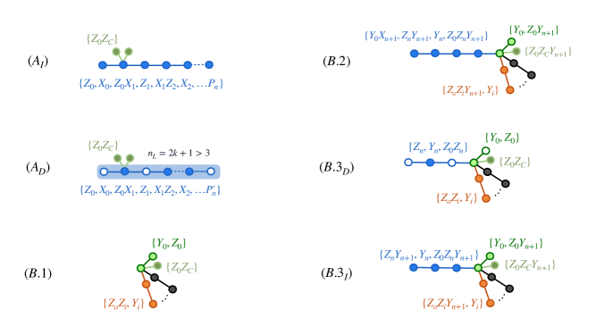
Let us start with graphs of type A, both with algebraic dependence and without. In this case, we simply need to choose a set of closest neighbour interacting Paulis,
| (46) |
together with a set of labels for additional control legs, where depends on the parity of and whether we are in the or instance. For all terms must be algebraically independent, so that depending on the parity of . For we can either have algebraic dependence or not. For , , whereas in , . With this, we can now prove that indeed this corresponds to the free-fermionic Lie algebra. We can limit to characterizing the Paulis lying on the path graph without legs of length 1, as controls can be removed at this point. From these, it is easy to define a set of majorana operators. In particular, we use Paulis in to do so, as this will not change the Lie algebra. Thus
| (47) | ||||
| (48) | ||||
| (49) | ||||
| (50) | ||||
| (51) | ||||
which satisfy
| (52) |
and thus
| (53) |
Hence, a basis for the Lie algebra is given by , where quadratic terms satisfy
| (54) |
The size of this basis then gives us that
| (55) |
which coincides with the dimension of . Finally, taking a basis of anti-symmetric matrices of size , it is easy to check that the structure constants of and are also the same, thus proving equality. The difference between and then comes from the fact that for the latter, the last Majorana operator is equal to the global parity operator.
For the rest of star-graph families, before giving the labeling, we will first introduce the following lemma regarding properties of certain colourings on the graph. With this lemma, proving the Lie algebra type will follow almost directly.
Lemma 6 (Odd colouring property)
If all generators of a star-type Pauli Lie algebra satisfy
| (56) |
for some Pauli , then every Pauli it holds that
| (57) |
For the set of of all Paulis generated by some colouring, we define the two subsets
| (58) |
In general, we have for , where and
| (59) |
As a consequence, we have that if and , then . This means that if we have a connected component , it follows that . This is because we can generate this by a nested sequence of generators. Since the graph has no loop, we can start at any element, and then take a commutator with a Pauli from that anti-commutes, until all Paulis were used exactly once. Now we consider the disconnected components. We have from Equation 59 that since . By iterative application we have that
| (60) |
This means that the Pauli satisfies the condition if the number of connected components is odd, and satisfies if is even. This gives the if and only if relationship that is desired by the lemma.
Having stated this, we can start discussing graphs B1. In this case, there is just one Clifford inequivalent class and we choose the labeling to be given by
| (61) |
where these sets label the central vertex and the first leg of length 1, all legs of length 2, and controls, respectively. Note that the central Pauli , is chosen so that as in the canonical definition in Appendix A in the definition of . Moreover, every vertex adjacent to the center is labeled by a symmetric Pauli , whereas non-adjacent vertices are labeled with an anti-symmetric Pauli . This precisely matches the defining condition for , i.e.,
| (62) |
Hence, since all our generators satisfy this condition, which is preserved under Lie product, all elements in our Lie algebra will, i.e.
| (63) |
For us to have equality as stated by Theorem 2, one would have to check that any element in can be generated by our Paulis. This, however, follows from Lemma 6. Given some , this can be written as a product of our generators, since these form a basis for the algebra of symplectic matrices of size . This follows from the same arguments as for finding the minimal number of qubits. Since independent Paulis are required to span the full algebra on qubits, in order to span one also needs at most symplectic generators, which is what we have. Thus, there is some colouring on the graph corresponding to . Since satisfies
| (64) |
with , then the colouring of must have an odd number of connected components. Now by Lemma 4 we know that such colourings can indeed be computed through nested commutators, thus concluding the proof that the Lie algebra spanned by this set of Paulis is indeed .
Given this labeling for the symplectic Lie algebra, one can easily find one for the family of graphs in B3, both for and . For the case of algebraic dependent generators, we can simply get our canonical labeling by adding , for . It is easy to see that if one takes the product of Paulis in the leg of length 1 and the innermost and outermost vertices of the newly created leg of length 3
| (65) |
Adding this additional Pauli allows us to generate any Pauli on qubits, i.e., promotes the Lie algebra to . That is because given a Pauli on qubits, we can always find a colouring which is computable, since in the case where has a colouring with an even number of connected components, then is a colouring with an odd number of connected components that yields the same Pauli.
If the generators are not algebraically dependent, by the rules that determine the minimal number of qubits, we must add a new qubit as well. Hence, instead of adding , we will introduce . Moreover, since every other Pauli commutes with , we can freely modify them so that the overall labeling for this case is
| (66) |
it is clear that now
| (67) |
so we cannot use the same argument as before. However, it suffices to prove it for one case, since the graph is the same for both. Furthermore, the last change was useful to see that as we stated in the main text, the map between and is given by , so that indeed the Lie algebra is the same in both cases, albeit in it is embedded in a bigger Hilbert space.
The other reason why appending to symmetric generators was because we can now easily find our canonical labeling for the last class of graphs Since we want to argue that this corresponds to the Lie algebra of anti-symmetric matrices , and all generators in Equation 66 are already anti-symmetric, we just need to add another anti-symmetric Pauli that breaks the symmetry with respect to . To that end, our new set of canonical generators will be given by
| (68) |
Then, since all generators satisfy the anti-symmetric condition, which is preserved under Lie product, we have
| (69) |
Like for the symplectic case, checking that any element in can be computed through nested commutators of our canonical generators is easy to see from Lemma 6 with . Again, for any Pauli satisfying
| (70) |
its colouring on the graph must have an odd number of connected components, and thus must be computable through nested commutators. This concludes our construction of all canonical Pauli sets for every Clifford inequivalent class, and serves as a proof of Theorem 2.
F.1 Clifford invariant form
In the previous section we mainly worked with the canonical definition for and . However, since Clifford operations do not change the Lie algebra, one could come up with a form that makes this explicit. Before, we introduced the canonical forms as
| (71) |
where for and for . If we perform a Clifford transformation, this turns into
| (72) |
As such, the statement becomes
| (73) | |||||
| (74) | |||||
| (75) | |||||
using . With this the action maps
| (76) |
This map still maps Paulis to Paulis upon conjugation up to phase. To see this, we can look at a particular generating set of the Clifford group, e.g., . On the one hand, since and , these act as ordinary Cliffords, mapping Paulis to Paulis. On the other hand, for the map , we have
| (77) |
However, for the relation that concerns us, this global phase becomes irrelevant. Additionally, we have that
| (78) |
i.e., the symmetric/anti-symmetric property is preserved under the action of this map. Additionally, we can map any (anti-)symmetric Pauli to any other (anti-)symmetric Pauli. For this, we can change by applying , by applying and , by applying . In order to change the number of Paulis we can use CNOTs to map . This then motivates the definition that is given in the main text.
Another interesting case in this regard, is that of the class where the canonical form is defined by
| (79) |
Again, applying a Clifford to the argument this becomes
| (80) | ||||
| (81) |
meaning
| (82) |
Thus, when the condition is satisfied
| (83) | ||||
Naturally, can become every non identity Pauli. Using only , it is possible to create every symmetric Pauli: to set it to , to set to , and CNOT on to create . Moreover, since all gates are real , which means that as well.
Next, we choose a , such that . Naturally, maps , . Now, choosing such that we get to the result we wanted. However, by design , meaning
| (84) | ||||
| (85) | ||||
| (86) | ||||
| (87) |
The current reduction requires . However, we can rewrite the commutation relation in an equivalent form
| (88) | ||||
| (89) |
as well as
| (90) |
using that . So if we define , we get that and the conditions that :
| (91) |
which shows that corresponds to a system with both a symplectic and an orthogonal relation. If we now use the symplectic relation we get
| (92) | ||||
| (93) | ||||
| (94) |
As such, defining , we have
| (95) | ||||
| (96) | ||||
| (97) |
using that . This means that the requirement for to be symmetric can be removed, by the outlined transformations. This concludes the condition of the Clifford invariant form given in the main text.