supplement.pdf

Small correlation is sufficient for optimal noisy quantum metrology

Abstract

We propose a class of metrological resource states whose quantum Fisher information scales optimally in both system size and noise rate. In these states, qubits are partitioned into sensing groups with relatively large correlations within a group but small correlations between groups. The states are obtainable from local Hamiltonian evolution, and we design a metrologically optimal and efficient measurement protocol utilizing time-reversed dynamics and single-qubit local measurements. Using quantum domino dynamics, we also present a protocol free of the time-reversal step that has an estimation error roughly twice the best possible value.

Introduction.— Quantum metrology Giovannetti et al. (2011); Degen et al. (2017); Pezzè et al. (2018); Pirandola et al. (2018) is the study of utilizing entanglement and other quantum effects to measure unknown data, such as gravitational waves Caves (1981); Yurke et al. (1986); LIGO Collaboration (2011, 2013), images Le Sage et al. (2013); Lemos et al. (2014); Tsang et al. (2016); Abobeih et al. (2019), magnetic fields Wineland et al. (1992); Bollinger et al. (1996); Leibfried et al. (2004); Taylor et al. (2008); Zhou et al. (2020), and time Rosenband et al. (2008); Appel et al. (2009); Ludlow et al. (2015); Kaubruegger et al. (2021); Marciniak et al. (2022). A typical metrological protocol involves initializing $N$ probes in a particular (possibly entangled) state, letting the value of an unknown quantity $\theta$ be imparted on the state, and estimating $\theta$ via a measurement. The Heisenberg limit (HL) Giovannetti et al. (2006) restricts the best-case estimation precision to scale inversely with the number $N$ of entangled probes, $\delta\theta\sim 1/N$.

The prototypical example of a “metrologically optimal” state is the Greenberger-Horne-Zeilinger (GHZ) state Giovannetti et al. (2006), which is used to attain the HL in estimating a $Z$-axis magnetic field in a noiseless $N$-spin system. Unfortunately, the useful but fragile quantum correlations of this state quickly break down in the presence of noise. Instead of attaining the HL, the optimal scaling in a generically noisy setting is the standard quantum limit (SQL), $\delta\theta\sim 1/\sqrt{N}$.

For quantum metrology to continue to bear fruit, it is important to quantify the performance of noise-robust metrological protocols not only in terms of the number of probes $N$ Giovannetti et al. (2006); Demkowicz-Dobrzański et al. (2012); Escher et al. (2011); Demkowicz-Dobrzański and Maccone (2014); Sekatski et al. (2017); Demkowicz-Dobrzański et al. (2017); Zhou et al. (2018), but also in terms of the noise rate $p$ of each probe. A more precise calculation for several models with non-negligible noise yields a precision of $\delta\theta\gtrsim\sqrt{p/N}$  Huelga et al. (1997); Demkowicz-Dobrzański et al. (2012); Escher et al. (2011); Demkowicz-Dobrzański and Maccone (2014); Zhou and Jiang (2021), meaning that reducing the noise rate $p$ can lead to a constant-factor improvement on top of the naive scaling with $1/\sqrt{N}$. In this Letter, we continue this direction and describe both criteria on and examples of protocols whose variance scales optimally  with both $N$ and $p$ (see Fig. 1 for a summary).

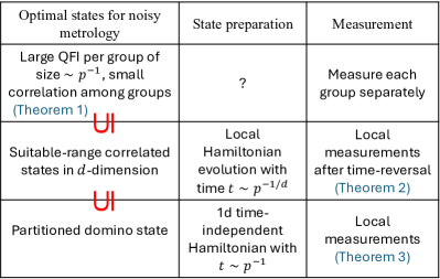
Figure 1: Three families of metrological optimal states and their corresponding preparation and measurement protocols. Each row is a special case of the previous row indicated by $\subseteq$, which has more efficient schemes for state preparation and measurement.

We show that achieving optimal scaling requires a careful tuning of the quantum correlation length. The extensive entanglement of the GHZ state is optimal only in the relatively noiseless setting of $pN\sim$ constant Hayashi et al. (2022), while unentangled states do not yield any $p$-dependent precision improvement. Interpolating between the two edge cases, we show that a “Goldilocks” amount of quantum correlation — quantified by a correlation length $M\sim 1/p$ — is required for optimality. This general theory corroborates previous numerical results Jarzyna and Demkowicz-Dobrzański (2013); Chabuda et al. (2020) that matrix product states with low bond dimension are optimal for strong noise.

We construct states that satisfy our criteria for optimality using local-Hamiltonian evolution, and present a provably efficient measurement protocol utilizing time-reversed evolution (similar to the Loschmidt echo Macrì et al. (2016)) and single-qubit measurements. We showcase our results by an example of optimal states generated by analytically solvable quantum domino dynamics Lee and Khitrin (2005); Yoshinaga et al. (2021), where local measurements without time reversal suffice for near-optimal performance.

Simple example—Our optimality conditions are stated for sensing a $Z$-axis magnetic field (with straightforward extension to any single-qudit Hamiltonian via local rotations) under arbitrary noise, but dephasing noise yields an illuminating warm-up example of the correlation that is required for optimality.

Let $N$ qubits, labeled by $i\in\Lambda$ with Pauli matrices $X_{i},Y_{i},Z_{i}$, be prepared in a state $\rho$, with each qubit $i$ undergoing the channel

$${\mathcal{D}}_{\theta,p}(\rho_{i})=(1-p)\mathrm{e}^{-\mathrm{i}\theta Z_{i}}\rho_{i}\mathrm{e}^{\mathrm{i}\theta Z_{i}}+pZ_{i}\mathrm{e}^{-\mathrm{i}\theta Z_{i}}\rho_{i}\mathrm{e}^{\mathrm{i}\theta Z_{i}}Z_{i}$$ (1)

for $0<p<1/2$. For simplicity, we assume $p>1/N$ (otherwise the noise is asymptotically negligible and the HL is achievable). One then measures the final state $\rho_{\theta}={\mathcal{D}}_{\theta,p}^{\otimes N}(\rho)$ to estimate $\theta$.

The estimation precision can be bounded by the state’s quantum Fisher information (QFI), $\delta\theta\geq 1/\sqrt{N_{\rm e}{\mathcal{F}}(\rho_{\theta})}$, via the quantum Cramér-Rao bound Helstrom (1976); Holevo (2011); Braunstein and Caves (1994); Barndorff-Nielsen and Gill (2000); Gill and Massar (2000); Paris (2009), saturable as the number of repeated experiments $N_{\rm e}\rightarrow\infty$. The QFI for the above example is bounded by Huelga et al. (1997); Escher et al. (2011); Demkowicz-Dobrzański et al. (2012); Zhou and Jiang (2021)

$${\mathcal{F}}(\rho_{\theta})\leq 4N/[1-(1-2p)^{2}]\sim N/p,$$ (2)

yielding the aforementioned scaling of $\delta\theta\sim\sqrt{p/N}$ . This QFI bound cannot be surpassed with arbitrary state preparation and measurement protocols, including quantum error correction Sekatski et al. (2017); Zhou et al. (2018); Demkowicz-Dobrzański et al. (2017).

This QFI bound can be saturated (up to a constant factor) by partitioning the $N$-qubit system into $N/M$ groups of $M$ qubits each (with $N/M$ assumed to be an integer for simplicity), tuning the groups’ size inversely with the noise rate, and repeating the GHZ protocol within each group. The corresponding quantum parity state, $\rho=\bigotimes_{I}\ket{\mathrm{GHZ}}_{I}\bra{\mathrm{GHZ}}_{I}$ with $\ket{\mathrm{GHZ}}_{I}=\frac{1}{\sqrt{2}}(\ket{0}^{\otimes M}+\ket{1}^{\otimes M})$, an instance of the quantum parity code  Shor (1995); Knill et al. (2000); Ralph et al. (2005), is optimal as follows.

In the noiseless limit $p=0$, each group $I$ gains a phase $M\theta$ independently that corresponds to a QFI $\sim M^{2}$, so the QFI of the entire state, equal to the sum of individual QFIs, scales as $(N/M)M^{2}=NM$. This scaling is robust against noise if $pM$ is upper bounded by a constant, because then dephasing noise will only cause the individual QFI to reduce by a constant factor Huelga et al. (1997). Therefore, Eq. (2) is saturated by tuning $M\sim 1/p$.

Sufficient condition for optimality.— The quantum parity state is not the only state that achieves the optimal QFI scaling $\sim N/p$, and such states need not be tensor-product states w.r.t. the partititoning into groups $I$ of size $M$. Any state with sufficiently large intra-group and sufficiently small inter-group correlations will do. This partitioning idea also extends to general noise channels.

We generalize the final state to be $\rho_{\theta}=\mathcal{N}_{\theta,p}^{\otimes N}(\rho)$, where $\mathcal{N}_{\theta,p}$ is the noisy channel depending on $\theta$, and the noise parameter $p$ quantifies the diamond distance between noiseless ($\mathcal{N}_{\theta,0}$) and noisy ($\mathcal{N}_{\theta,p}$) evolutions (SM, , Sec. 5.1).

Before stating our general sufficient condition (see SM for the proof), we first introduce some notation. For any state $\sigma$ and operators $A,B$, define the expectation $\left\langle A\right\rangle_{\sigma}:=\mathrm{tr}\left(\sigma A\right)$, the correlation function

$$C_{\sigma}(A,B):=\mathrm{tr}\left(\sigma AB\right)-\mathrm{tr}\left(\sigma A\right)\mathrm{tr}\left(\sigma B\right),$$ (3)

and the variance $\left\langle\Delta A^{2}\right\rangle_{\sigma}=C_{\sigma}(A,A)$. Let $\rho_{I}$ be the reduced density matrix (RDM) of group $I$ before sensing, and let $\rho_{I,\theta}$ ($\rho^{(0)}_{I,\theta}$) be the noisy (noiseless) RDM after sensing. We use $A_{I}$ to indicate that operator $A$ acts inside group $I$, and denote the operator norm by $\left\lVert\cdot\right\rVert$.

Theorem 1.

For any given $p$, choose any $M<N$ with

$$M\leq c_{\rm no}/p,$$ (4)

where $c_{\rm no}$ is a positive constant, and partition the qubits as above. Given any state $\rho$, suppose for any group $I$, its QFI in the noiseless limit is large,

$${\mathcal{F}}\left(\rho^{(0)}_{I,\theta}\right)\sim M^{2},$$ (5)

and its correlations with other groups are small, i.e.,

$$\sum_{J:J\notin\mathcal{S}_{I}}\left\lvert C_{\rho}(A_{I},A_{J})\right\rvert\lesssim M^{-2}{\max_{J}\left\lVert A_{J}\right\rVert^{2}},$$ (6)

where $\mathcal{S}_{I}$ is some set of groups containing a finite (independent of $N,p,M$) number of elements (including $I$) that may have large correlation with $I$. Then there exists an observable ${\mathcal{O}}=\sum_{I}{\mathcal{O}}_{I}$ such that

$${\mathcal{F}}(\rho_{\theta})\geq\frac{1}{\left\langle\Delta{\mathcal{O}}^{2}\right\rangle_{\rho_{\theta}}}\left(\partial_{\theta}\left\langle{\mathcal{O}}\right\rangle_{\rho_{\theta}}\right)^{2}\sim NM.$$ (7)

Eq. (7) implies the optimal QFI scaling (Eq. (2)) is saturated by choosing $M\sim 1/p$. Moreover, ${\mathcal{O}}$ here represents the optimal observable to measure, and $\left\langle\Delta{\mathcal{O}}^{2}\right\rangle_{\rho_{\theta}}$ and $\left\langle{\mathcal{O}}\right\rangle_{\rho_{\theta}}$ represent its variance and expectation value w.r.t. $\rho_{\theta}$, respectively (see, e.g., Ref. Pezzé and Smerzi (2009) for the signal-to-noise-ratio lower bound on QFI that we use in Eq. (7)). The optimal observable is a sum of individual observables ${\mathcal{O}}_{I}$ on each group, and individual measurements on each group suffice to achieve the optimal QFI. The two conditions generalize the quantum parity state example: (i) Eq. (5) requires that each group has the asymptotically optimal QFI $\sim M^{2}$ , and (ii) Eq. (6) requires each group to have a large correlation with a finite number of other groups, which guarantees the linear scaling of the QFI with respect to $M$.

Locally generated optimal states.— Our sufficient condition is naturally satisfied by states generated by local Hamiltonian evolution. Suppose the qubits lie on vertices of a $d$-dimensional square lattice, start from $\ket{\bm{0}}:=\ket{0}^{\otimes N}$, and evolve to a state $\ket{\psi}=U\ket{\bm{0}}$ by a unitary $U$ generated by a (possibly time-dependent) local Hamiltonian for time $T$. Such evolution is quasi-causal because it satisfies the following Lieb–Robinson bound Lieb and Robinson (1972); Chen et al. (2023): if an operator $A$ acts within set $S\subseteq\Lambda$, then, in the Heisenberg picture,

$$A(T):=U^{\dagger}AU\approx\widetilde{A}_{\widetilde{S}},$$ (8)

i.e., $A(T)$ can be approximated (up to small error) by an operator $\widetilde{A}$ that is strictly supported in the “light cone” region

$$\widetilde{S}:=\{i\in\Lambda:\mathsf{d}(i,S)\leq T\},$$ (9)

which contains all vertices within distance $T$ to $S$. Here, $T$ is rescaled such that the Lieb–Robinson velocity Chen et al. (2023) is set to $1$, and $\mathsf{d}(\cdot,\cdot)$ is the distance function with $\mathsf{d}(i,S)=\min_{j\in S}\mathsf{d}(i,j)$. For illustrative purpose, we assume Eq. (8) is exact from now on, with the rigorous treatment given elsewhere SM .

The state $\rho=\ket{\psi}\bra{\psi}=U\ket{\bm{0}}\bra{\bm{0}}U^{\dagger}$ has correlation length at most $2T$ Bravyi et al. (2006) because faraway light cones do not intersect. Therefore, it naturally satisfies Eq. (6) if each group $I$ is chosen to be an $L\times\cdots\times L$ hypercube with $L=M^{1/d}\gtrsim T$, as sketched in Fig. 2. We choose $T\sim L$ so that qubits within each group are sufficiently correlated so as to satisfy Eq. (5) Chu et al. (2023).

Based on Theorem 1, the class of optimal metrological states contains any state $\rho$ defined above with large intra-group $ZZ$ correlation:

$$C_{\rho}(Z_{I},Z_{I})\geq c_{Z}L^{d}T^{d},$$ (10)

corresponding to Eq. (5) , where $Z_{I}=\sum_{i\in I}Z_{i}$ and $c_{Z}\sim 1$. Such optimal states are efficiently preparable by definition, but it is still demanding to develop efficient measurement schemes because the measurement observable used in Theorem 1, although separate for each group, can be difficult to implement when the group size is large.

Local measurement scheme with time-reversal.— For any such state $\rho$, we propose a local measurement scheme by only assuming the ability to time-reverse the evolution $U$ (e.g., by changing the sign of the generating Hamiltonian). Namely, after sensing, one applies a unitary $U_{\rm rev}:=U^{\dagger}\mathrm{e}^{\mathrm{i}\theta_{\rm pr}Z}$ ($Z:=\sum_{i}Z_{i}$) to the state $\rho_{\theta}$, and then measures in the computational basis before post-processing the data. Here, $\theta_{\rm pr}$ represents prior knowledge of $\theta$, such that $\tilde{\theta}:=\theta-\theta_{\rm pr}$ satisfies $|\tilde{\theta}|\sim L^{-d}$ . The idea comes from the Loschmidt echo protocol working in the noiseless case Macrì et al. (2016), where one processes the measurement data by simply computing the final probability of returning to $\ket{\bm{0}}$:

$$\mathsf{P}_{\rm echo}:=\left\lvert\bra{\bm{0}}U^{\dagger}\mathrm{e}^{-\mathrm{i}\tilde{\theta}Z}U\ket{\bm{0}}\right\rvert^{2}\!=1-\frac{\tilde{\theta}^{2}}{4}\!\mathcal{F}(\rho_{\theta})+\mathrm{O}(\tilde{\theta}^{4}).$$ (11)

The measurement is optimal, i.e., the corresponding classical Fisher information $\frac{1}{\Delta\mathsf{P}_{\rm echo}^{2}}\left(\partial_{\theta}\mathsf{P}_{\rm echo}\right)^{2}\approx\mathcal{F}(\rho_{\theta})$ at small $\tilde{\theta}$, where $\Delta\mathsf{P}_{\rm echo}^{2}=\mathsf{P}_{\rm echo}(1-\mathsf{P}_{\rm echo})$ is the variance of a Bernoulli random variable with probability $\mathsf{P}_{\rm echo}$.

However, the global projective measurement $\ket{\bm{0}}\bra{\bm{0}}$ in Eq. (11) is not robust against noise. To guarantee robustness, we post-process the data in the following way. After the computational-basis measurement, one instead computes projections $P_{\widetilde{I}}:=\bigotimes_{i\in\widetilde{I}}\ket{0}_{i}\bra{0}$ onto small regions $\widetilde{I}$ (defined via Eq. (9)), so that the overall observable is $\left\langle{\mathcal{O}}_{\rm rev}\right\rangle_{\rho_{\theta}}$ with ${\mathcal{O}}_{\rm rev}:=\sum_{I}\widetilde{P}_{I}:=\sum_{I}U_{\rm rev}^{\dagger}P_{\widetilde{I}}U_{\rm rev}$. (We often omit the identity operator on the rest of the system for simplicity, e.g., here $P_{\widetilde{I}}$ means $P_{\widetilde{I}}\otimes\mathrm{id}$.) This time-reversal local measurement scheme is asymptotically optimal.

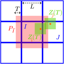
Figure 2: A coarse-grained sketch for the time-reversal local measurement protocol in 2d, where the underlying lattice is not shown. There is an observable $P_{\widetilde{I}}$ for each group $I$ after the time-reversal $U_{\rm rev}$, whose expectation is only affected by dynamics in the neighboring groups since $L>T$. As a crucial step to establish large sensitivity Eq. (16), we show terms like $\bra{\bm{0}}[Z_{I}(T),[Z_{J}(T),P_{\widetilde{I}}]]\ket{\bm{0}}$ contribute subdominantly in Eq. (Small correlation is sufficient for optimal noisy quantum metrology), using the fact that only sites $i\in I,j\in J$ (orange dots) whose operators $Z_{i}(T)$ and $Z_{j}(T)$ (green regions) have overlapping support contribute to these terms.

Theorem 2.

For any $p$, choose $L=M^{1/d}$ such that Eq. (4) holds for some constant $c_{\rm no}$ (which is not necessarily the same constant in Theorem 1). For any locally generated state $\rho$ satisfying Eq. (10), there exist constants $C>c>1$ determined by $c_{Z}$ and $d$, such that for any $C\geq L/T\geq c$,

$$\frac{1}{\left\langle\Delta{\mathcal{O}}^{2}_{\rm rev}\right\rangle_{\rho_{\theta}}}\left(\partial_{\theta}\left\langle{\mathcal{O}}_{\rm rev}\right\rangle_{\rho_{\theta}}\right)^{2}\sim NL^{d}.$$ (12)

Note that the observable ${\mathcal{O}}_{\rm rev}$ here is independent of $p$, in contrast to ${\mathcal{O}}$ in Theorem 1 that is a function of $p$. We sketch the idea of Theorem 2 and leave the full proof to SM . Note that all approximations “$\approx$” below stem from the light-cone approximation in Eq. (8).

Focusing on $d=2$ (generalization is straightforward) as shown in Fig. 2 and recalling that $|\tilde{\theta}|\sim L^{-2}$ and $T\sim L$, we first expand in the noiseless case,

$$\langle\widetilde{P}_{I}\rangle_{\rho_{\theta}^{(0)}} =\bra{\bm{0}}\mathrm{e}^{\mathrm{i}\tilde{\theta}Z(T)}P_{\widetilde{I}}\mathrm{e}^{-\mathrm{i}\tilde{\theta}Z(T)}\ket{\bm{0}}$$

$$=1-\frac{\tilde{\theta}^{2}}{2}\bra{\bm{0}}[Z(T),[Z(T),P_{\widetilde{I}}]]\ket{\bm{0}}+\cdots.$$ (13)

The first-order term vanishes similarly as Eq. (11), and we show that the second-order term is $\sim\tilde{\theta}^{2}L^{4}$. (Note that we have required that $|\tilde{\theta}|$ is sufficiently large to guarantee that the second-order derivative is dominant.) We expand $Z=\sum_{J}Z_{J}$ and observe that only $J=I$ or neighbors of $I$ contribute, because otherwise $[Z_{J}(T),P_{\widetilde{I}}]=0$ since they do not overlap in space from Eq. (8). Furthermore, when $L/T$ is a sufficiently large constant, the coefficient is dominated by the term

$$\bra{\bm{0}}[Z_{I}(T),[Z_{I}(T),P_{\widetilde{I}}]]\ket{\bm{0}}\\ \approx 2\,C_{\rho}(Z_{I},Z_{I})\geq 2c_{Z}L^{2}T^{2},$$ (14)

which can be verified from direct computation and Eq. (10). The reason is that the sum of all other terms is $\lesssim LT^{3}$, which becomes subdominant when $L/T$ is sufficiently large. To show this, we note that for $i\in I,j\in J\neq I$,

$$\bra{\bm{0}}[Z_{i}(T),[Z_{j}(T),P_{\widetilde{I}}]]\ket{\bm{0}}\approx 0,$$ (15)

unless the two sites are close ($\mathrm{d}(i,j)\leq 2T$), as shown in Fig. 2. Then the sum of Eq. (15) over $i,j$ is bounded by $\sum_{j\text{ close to }I}\sum_{i\text{ close to }j}\lesssim LT\cdot T^{2}$.

Above we showed, at sufficiently large $L/T$, the second-order coefficient in Eq. (Small correlation is sufficient for optimal noisy quantum metrology) is $\sim L^{4}$. This guarantees $-\partial_{\theta}\langle\widetilde{P}_{I}\rangle_{\rho_{\theta}^{(0)}}\sim\tilde{\theta}\times\text{[the second-order coefficient]}\sim L^{2}$, and thus

$$\partial_{\theta}\left\langle{\mathcal{O}}_{\rm rev}\right\rangle_{\rho_{\theta}^{(0)}}\sim N.$$ (16)

(Note that the higher orders of $\tilde{\theta}$ in Eq. (Small correlation is sufficient for optimal noisy quantum metrology) are safely ignored by similar locality analysis.) Since faraway groups are hardly correlated,

$$\left\langle\Delta{\mathcal{O}}^{2}_{\rm rev}\right\rangle_{\rho_{\theta}^{(0)}}\sim\sum_{I}\big{\langle}\Delta\widetilde{P}_{I}^{2}\big{\rangle}_{\rho_{\theta}^{(0)}}\lesssim N/L^{2},$$ (17)

leading to Eq. (12) for the noiseless case.

Finally, we consider the noisy case $p>0$. Eq. (17) still holds (where $\rho_{\theta}^{(0)}$ is replaced with $\rho_{\theta}$) because adding noise does not create long-range correlation Poulin (2010). It then remains to show Eq. (16) is also robust. For illustrative purposes, we focus on dephasing noise here, i.e., $\mathcal{N}_{\theta,p}={\mathcal{D}}_{\theta,p}$, yielding

$$\left\lvert\partial_{\theta}\big{(}\big{\langle}{\widetilde{P}_{I}}\big{\rangle}_{\rho_{\theta}}-\big{\langle}{\widetilde{P}_{I}}\big{\rangle}_{\rho_{\theta}^{(0)}}\big{)}\right\rvert=\left\lvert\big{\langle}{\big{[}Z,{\mathcal{D}}_{0,p}^{\otimes N}(\widetilde{P}_{I})-\widetilde{P}_{I}}\big{]}\big{\rangle}_{\rho_{\theta}^{(0)}}\right\rvert$$

$$\lesssim L^{2}\left\lVert{\mathcal{D}}_{0,p}^{\otimes c_{0}L^{2}}(\widetilde{P}_{I})-\widetilde{P}_{I}\right\rVert\lesssim L^{4}p,$$ (18)

where we recall that the dual map of the dephasing noise ${\mathcal{D}}_{0,p}$ is itself, and use the locality of $\widetilde{P}_{I}$ to restrict the channel to a region of size $c_{0}L^{2}$ with $c_{0}\sim 1$. Taking $pL^{2}\leq c_{\rm no}$ and $c_{\rm no}$ sufficiently small guarantees the contribution from noise to Eq. (16) is subdominant relative to the noiseless result.

Quantum domino dynamics with local measurement.— We have shown that any state generated by local dynamics with correlations of the form Eq. (10) is metrologically optimal when $L^{d}\sim 1/p$. Here we present a simple application of this framework using quantum domino dynamics Lee and Khitrin (2005); Yoshinaga et al. (2021).

Consider the $3$-local spin-chain Hamiltonian that flips a spin only if its two neighbors are anti-aligned,

$$H_{\rm do}=\frac{1}{2}\sum_{i=2}^{N-1}X_{i}(1-Z_{i-1}Z_{i+1}),$$ (19)

which can be engineered as the effective Hamiltonian for the transerve-field Ising model at weak $X$ field Lee and Khitrin (2005). The vacuum $\ket{\bm{0}}$ is an eigenstate of $H_{\rm do}$, and, more generally, the number of domain walls (DWs)—transitions from $\ket{0}$ to $\ket{1}$ or vice versa—is conserved. If the system starts from the initial state $\ket{1_{1}}:=\ket{10\cdots 0}$, it only traverses the state space with one DW $\mathrm{e}^{-\mathrm{i}TH_{\rm do}}\ket{1_{1}}=\sum_{i=1}^{N}a_{i}\ket{1_{i}}$, where $\ket{1_{i}}$ is the state with $1$ on the first $i$ qubits and $0$ on the rest, and where the coefficients $a_{i}$ are determined by $T$. This single-particle hopping process of the DW justifies the name “domino”. Before $T\gtrsim N$ (i.e., when the DW propagates to the right), $a_{i}$ is centered around $i=vT$ with a velocity $v$. Then, an initial state $\ket{+}_{1}\otimes|\bm{0}\rangle$ would evolve to

$$\ket{\psi_{\rm do}}:=\mathrm{e}^{-\mathrm{i}TH_{\rm do}}\ket{+}_{1}\otimes|\bm{0}\rangle=\frac{1}{\sqrt{2}}\left(\ket{\bm{0}}+\sum_{i=1}^{N}a_{i}\ket{1_{i}}\right),$$ (20)

which is roughly a GHZ-like state on the left $\sim vT$ qubits (with other qubits in state $\ket{0}$), useful for metrology Yoshinaga et al. (2021).

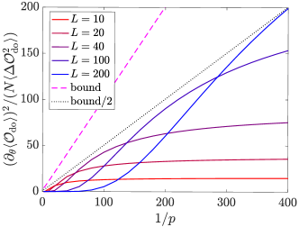
Figure 3: Optimal noisy metrology for $N=200$ qubits under dephasing, using partitioned domino state Eq. (21) generated from quantum domino dynamics, and local measurements ${\mathcal{O}}_{\rm do}$ of the form Eq. (25). The $y$-axis quantifies $(\delta\theta)^{-2}/N$ for local estimation at $\theta\approx 0$. For each solid line, the spin chain is divided to $N/L$ groups each of size $L$, and the generating time $T\sim L$ is suitably chosen (see SM for details). For any noise probability $p\ll 1$ in Eq. (1), by choosing suitable $T$ and $L$, the performance approaches the bound Eq. (2) (pink dashed line) up to a factor $\approx 2$.

Adapting the domino dynamics to our partition framework, we propose to evolve the initial state containing one $\ket{+}$ in every $L$ qubits:

$$\ket{\Psi_{\rm do}}:=\mathrm{e}^{-\mathrm{i}TH_{\rm do}}\left(\ket{+}_{L}\otimes\ket{+}_{2L}\otimes\cdots\right)\otimes|\bm{0}\rangle_{\rm rest}.$$ (21)

This final state, which we call the partitioned domino state, satisfies Eq. (10) for $T\lesssim L$, because the two DWs of each $\ket{+}$ roughly propagate in opposite directions with constant velocity. We numerically study noisy metrology using $\ket{\Psi_{\rm do}}$ on a chain of $200$ qubits, and Fig. 3 shows the results. Remarkably, this protocol is not only optimal asymptotically, but also quantitatively. By adjusting $L$ for different $p$, the precision $(\delta\theta)^{2}$ is only roughly twice larger than the ultimate limit Eq. (2).

Besides having nearly the same metrological power as the quantum parity state, the domino-state protocol requires only local measurements without any time-reversed evolution. To show this, we focus first on the simplest one-DW case with state Eq. (20). In SM , we prove the following for various combinations $\mathcal{N}_{\theta,p}$ of $\theta$-imparting unitary evolution and a general noisy channel.

Theorem 3.

In a rotated local basis (i.e., redefining states $\ket{1}_{i}$ with extra phases) such that $\mathrm{Arg}(a_{i})=-\frac{\pi}{2}(1+i)-2\theta_{\rm pr}i$, define the measurement observable

$${\mathcal{O}}_{\rm do}:=\sum_{vT/2\leq i\leq 2vT}|a_{i}|\mathbf{Y}_{i},$$ (22)

where $\mathbf{Y}_{i}:=\bigotimes_{j=1}^{i}Y_{j}$. If

$$\sum_{vT/2\leq i\leq 2vT}|a_{i}|^{2}\geq c_{\rm do}\sim 1,$$ (23)

then

$$\frac{1}{\left\langle\Delta{\mathcal{O}}^{2}_{\rm do}\right\rangle_{\rho_{\theta}}}\left(\partial_{\theta}\left\langle{\mathcal{O}}_{\rm do}\right\rangle_{\rho_{\theta}}\right)^{2}\sim T^{2},$$ (24)

where $\rho_{\theta}=\mathcal{N}_{\theta,p}^{\otimes N}(\ket{\psi_{\rm do}}\bra{\psi_{\rm do}})$ with noise $p\leq c_{\rm do}/(vT)$ for a constant $c_{\rm do}$.

Eq. (22) can be realized by $Y$-basis local measurements with efficient classical post-processing. The condition Eq. (23) means that $|a_{i}|^{2}$, as a probability distribution, is concentrated around $vT$, which can be verified from the exact solution (Bessel function) of $a_{i}$ Roubert et al. (2010). The idea is as follows. $\ket{\psi_{\rm do}}$ is roughly a superposition of GHZ states $\ket{\mathrm{GHZ}}_{1\cdots i}\otimes\ket{\bm{0}}$ of different size $i$. For each GHZ state, the canonical observable is $\mathbf{Y}_{i}$. The problem is that each such observable does not have large sensitivity, i.e., $\partial_{\theta}\left\langle\mathbf{Y}_{i}\right\rangle\sim|a_{i}|\ll 1$, because the DW wave packet spreads. To overcome this, we use a suitable linear combination of them, namely, ${\mathcal{O}}_{\rm do}$, to accumulate the small derivatives into $\partial_{\theta}{\mathcal{O}}_{\rm do}\sim\sum_{i}|a_{i}|^{2}\sim 1$. It turns out this linear combination does not lead to large variance of ${\mathcal{O}}_{\rm do}$ due to the lack of interference among the GHZ states in $\ket{\psi_{\rm do}}$, making ${\mathcal{O}}_{\rm do}$ a suitable observable.

Generalizing the idea, the observable we use in Fig. 3 for state Eq. (21) is of the form

$$\bigg{(}\sum_{i,j}b_{i,j}\mathbf{Y}_{i,j}\bigg{)}\otimes\bigg{(}\sum_{i,j}b_{i,j}\mathbf{Y}_{L+i,L+j}\bigg{)}\otimes\cdots,$$ (25)

where the real coefficients $b_{i,j}$ come from simulating the two-DW subspace, which only requires polynomial (in $L$) resource of classical computation. See SM for details.

Spin-squeezing.— We show in SM that certain types of spin-squeezed states (SSS) Kitagawa and Ueda (1993); Ma et al. (2011), though demanding to prepare Block et al. (2023), are another example of metrological optimality. Although spin squeezing is beyond the regime of Theorem 1, certain boundedness of correlation functions is also sufficient, suggesting the general usefulness of correlation bounds for noisy metrology.

Discussion.— In this work, we prove sufficient conditions for optimal noisy metrology and illustrate them with several examples, from simple quantum parity states to quantum domino dynamics and spin-squeezed states.

Beyond state optimality, we also address the problem of efficient measurement schemes for metrology. In particular, the domino example suggests that local measurements apply to wider sensing scenarios beyond GHZ: Although a local measurement scheme that exactly saturates the QFI Liu et al. (2023) may not exist, the QFI can still be saturated up to a moderate prefactor. The example also raises an interesting connection between quantum metrology and many-body dynamics, hinting at the possibility of other natural (e.g. time-independent) Hamiltonian dynamics generating high-QFI states in higher spatial dimensions.

Acknowledgements.— C.Y. was supported by the Department of Energy under Quantum Pathfinder Grant DE-SC0024324. S.Z. acknowledges funding provided by Perimeter Institute for Theoretical Physics, a research institute supported in part by the Government of Canada through the Department of Innovation, Science and Economic Development Canada and by the Province of Ontario through the Ministry of Colleges and Universities. VVA thanks Ryhor Kandratsenia and Olga Albert for providing daycare support throughout this work.

in 1,…,0 See pages \x, of supplement.pdf

References

- Giovannetti et al. (2011) Vittorio Giovannetti, Seth Lloyd, and Lorenzo Maccone, “Advances in quantum metrology,” Nature photonics 5, 222–229 (2011).
- Degen et al. (2017) C. L. Degen, F. Reinhard, and P. Cappellaro, “Quantum sensing,” Rev. Mod. Phys. 89, 035002 (2017).
- Pezzè et al. (2018) Luca Pezzè, Augusto Smerzi, Markus K. Oberthaler, Roman Schmied, and Philipp Treutlein, “Quantum metrology with nonclassical states of atomic ensembles,” Rev. Mod. Phys. 90, 035005 (2018).
- Pirandola et al. (2018) Stefano Pirandola, Bhaskar Roy Bardhan, Tobias Gehring, Christian Weedbrook, and Seth Lloyd, “Advances in photonic quantum sensing,” Nat. Photonics. 12, 724 (2018).
- Caves (1981) Carlton M. Caves, “Quantum-mechanical noise in an interferometer,” Phys. Rev. D 23, 1693–1708 (1981).
- Yurke et al. (1986) Bernard Yurke, Samuel L. McCall, and John R. Klauder, “Su(2) and su(1,1) interferometers,” Phys. Rev. A 33, 4033–4054 (1986).
- LIGO Collaboration (2011) LIGO Collaboration, “A gravitational wave observatory operating beyond the quantum shot-noise limit,” Nature Physics 7, 962–965 (2011).
- LIGO Collaboration (2013) LIGO Collaboration, “Enhanced sensitivity of the ligo gravitational wave detector by using squeezed states of light,” Nature Photonics 7, 613–619 (2013).
- Le Sage et al. (2013) David Le Sage, Koji Arai, David R Glenn, Stephen J DeVience, Linh M Pham, Lilah Rahn-Lee, Mikhail D Lukin, Amir Yacoby, Arash Komeili, and Ronald L Walsworth, “Optical magnetic imaging of living cells,” Nature 496, 486–489 (2013).
- Lemos et al. (2014) Gabriela Barreto Lemos, Victoria Borish, Garrett D Cole, Sven Ramelow, Radek Lapkiewicz, and Anton Zeilinger, “Quantum imaging with undetected photons,” Nature 512, 409–412 (2014).
- Tsang et al. (2016) Mankei Tsang, Ranjith Nair, and Xiao-Ming Lu, “Quantum theory of superresolution for two incoherent optical point sources,” Physical Review X 6, 031033 (2016).
- Abobeih et al. (2019) MH Abobeih, J Randall, CE Bradley, HP Bartling, MA Bakker, MJ Degen, M Markham, DJ Twitchen, and TH Taminiau, “Atomic-scale imaging of a 27-nuclear-spin cluster using a quantum sensor,” Nature 576, 411–415 (2019).
- Wineland et al. (1992) D. J. Wineland, J. J. Bollinger, W. M. Itano, F. L. Moore, and D. J. Heinzen, “Spin squeezing and reduced quantum noise in spectroscopy,” Phys. Rev. A 46, R6797–R6800 (1992).
- Bollinger et al. (1996) J. J. Bollinger, Wayne M. Itano, D. J. Wineland, and D. J. Heinzen, “Optimal frequency measurements with maximally correlated states,” Phys. Rev. A 54, R4649–R4652 (1996).
- Leibfried et al. (2004) D. Leibfried, M. D. Barrett, T. Schaetz, J. Britton, J. Chiaverini, W. M. Itano, J. D. Jost, C. Langer, and D. J. Wineland, “Toward heisenberg-limited spectroscopy with multiparticle entangled states,” Science 304, 1476–1478 (2004).
- Taylor et al. (2008) JM Taylor, Paola Cappellaro, L Childress, Liang Jiang, Dmitry Budker, PR Hemmer, Amir Yacoby, R Walsworth, and MD Lukin, “High-sensitivity diamond magnetometer with nanoscale resolution,” Nature Physics 4, 810–816 (2008).
- Zhou et al. (2020) Hengyun Zhou, Joonhee Choi, Soonwon Choi, Renate Landig, Alexander M Douglas, Junichi Isoya, Fedor Jelezko, Shinobu Onoda, Hitoshi Sumiya, Paola Cappellaro, et al., “Quantum metrology with strongly interacting spin systems,” Physical review X 10, 031003 (2020).
- Rosenband et al. (2008) Till Rosenband, DB Hume, PO Schmidt, Chin-Wen Chou, Anders Brusch, Luca Lorini, WH Oskay, Robert E Drullinger, Tara M Fortier, Jason E Stalnaker, et al., “Frequency ratio of al+ and hg+ single-ion optical clocks; metrology at the 17th decimal place,” Science 319, 1808–1812 (2008).
- Appel et al. (2009) Jürgen Appel, Patrick Joachim Windpassinger, Daniel Oblak, U Busk Hoff, Niels Kjærgaard, and Eugene Simon Polzik, “Mesoscopic atomic entanglement for precision measurements beyond the standard quantum limit,” Proceedings of the National Academy of Sciences 106, 10960–10965 (2009).
- Ludlow et al. (2015) Andrew D Ludlow, Martin M Boyd, Jun Ye, Ekkehard Peik, and Piet O Schmidt, “Optical atomic clocks,” Reviews of Modern Physics 87, 637 (2015).
- Kaubruegger et al. (2021) Raphael Kaubruegger, Denis V Vasilyev, Marius Schulte, Klemens Hammerer, and Peter Zoller, “Quantum variational optimization of ramsey interferometry and atomic clocks,” Physical review X 11, 041045 (2021).
- Marciniak et al. (2022) Christian D Marciniak, Thomas Feldker, Ivan Pogorelov, Raphael Kaubruegger, Denis V Vasilyev, Rick van Bijnen, Philipp Schindler, Peter Zoller, Rainer Blatt, and Thomas Monz, “Optimal metrology with programmable quantum sensors,” Nature 603, 604–609 (2022).
- Giovannetti et al. (2006) Vittorio Giovannetti, Seth Lloyd, and Lorenzo Maccone, “Quantum metrology,” Phys. Rev. Lett. 96, 010401 (2006).
- Demkowicz-Dobrzański et al. (2012) Rafał Demkowicz-Dobrzański, Jan Kołodyński, and Mădălin Guţă, “The elusive heisenberg limit in quantum-enhanced metrology,” Nature communications 3, 1063 (2012).
- Escher et al. (2011) BM Escher, Ruynet Lima de Matos Filho, and Luiz Davidovich, “General framework for estimating the ultimate precision limit in noisy quantum-enhanced metrology,” Nature Physics 7, 406–411 (2011).
- Demkowicz-Dobrzański and Maccone (2014) Rafal Demkowicz-Dobrzański and Lorenzo Maccone, “Using entanglement against noise in quantum metrology,” Physical review letters 113, 250801 (2014).
- Sekatski et al. (2017) Pavel Sekatski, Michalis Skotiniotis, Janek Kołodyński, and Wolfgang Dür, “Quantum metrology with full and fast quantum control,” Quantum 1, 27 (2017).
- Demkowicz-Dobrzański et al. (2017) Rafał Demkowicz-Dobrzański, Jan Czajkowski, and Pavel Sekatski, “Adaptive quantum metrology under general markovian noise,” Phys. Rev. X 7, 041009 (2017).
- Zhou et al. (2018) Sisi Zhou, Mengzhen Zhang, John Preskill, and Liang Jiang, “Achieving the heisenberg limit in quantum metrology using quantum error correction,” Nature communications 9, 78 (2018).
- Huelga et al. (1997) S. F. Huelga, C. Macchiavello, T. Pellizzari, A. K. Ekert, M. B. Plenio, and J. I. Cirac, “Improvement of frequency standards with quantum entanglement,” Phys. Rev. Lett. 79, 3865–3868 (1997).
- Zhou and Jiang (2021) Sisi Zhou and Liang Jiang, “Asymptotic theory of quantum channel estimation,” PRX Quantum 2, 010343 (2021).
- Note (1) We say a family of quantum states as functions of and is optimal, if and only if for any and , there exists a universal constant such that the QFI .
- Hayashi et al. (2022) Masahito Hayashi, Zi-Wen Liu, and Haidong Yuan, “Global heisenberg scaling in noisy and practical phase estimation,” Quantum Science and Technology 7, 025030 (2022).
- Jarzyna and Demkowicz-Dobrzański (2013) Marcin Jarzyna and Rafał Demkowicz-Dobrzański, “Matrix product states for quantum metrology,” Phys. Rev. Lett. 110, 240405 (2013).
- Chabuda et al. (2020) Krzysztof Chabuda, Jacek Dziarmaga, Tobias J Osborne, and Rafał Demkowicz-Dobrzański, “Tensor-network approach for quantum metrology in many-body quantum systems,” Nature communications 11, 250 (2020).
- Macrì et al. (2016) Tommaso Macrì, Augusto Smerzi, and Luca Pezzè, “Loschmidt echo for quantum metrology,” Phys. Rev. A 94, 010102 (2016).
- Lee and Khitrin (2005) Jae-Seung Lee and A. K. Khitrin, “Stimulated wave of polarization in a one-dimensional ising chain,” Phys. Rev. A 71, 062338 (2005).
- Yoshinaga et al. (2021) Atsuki Yoshinaga, Mamiko Tatsuta, and Yuichiro Matsuzaki, “Entanglement-enhanced sensing using a chain of qubits with always-on nearest-neighbor interactions,” Phys. Rev. A 103, 062602 (2021).
- Helstrom (1976) C W Helstrom, “Quantum detection and estimation theory,” (1976).
- Holevo (2011) Alexander S Holevo, Probabilistic and statistical aspects of quantum theory, Vol. 1 (Springer Science & Business Media, 2011).
- Braunstein and Caves (1994) Samuel L. Braunstein and Carlton M. Caves, “Statistical distance and the geometry of quantum states,” Phys. Rev. Lett. 72, 3439–3443 (1994).
- Barndorff-Nielsen and Gill (2000) Ole E Barndorff-Nielsen and Richard D Gill, “Fisher information in quantum statistics,” Journal of Physics A: Mathematical and General 33, 4481 (2000).
- Gill and Massar (2000) Richard D Gill and Serge Massar, “State estimation for large ensembles,” Physical Review A 61, 042312 (2000).
- Paris (2009) Matteo G. A. Paris, “Quantum estimation for quantum technology,” International Journal of Quantum Information 07, 125–137 (2009).
- Note (2) We use and to denote and , respectively, where are positive constants.
- Shor (1995) Peter W. Shor, “Scheme for reducing decoherence in quantum computer memory,” Phys. Rev. A 52, R2493–R2496 (1995).
- Knill et al. (2000) E. Knill, R. Laflamme, and G. Milburn, “Efficient linear optics quantum computation,” arXiv:quant-ph/0006088 (2000).
- Ralph et al. (2005) T. C. Ralph, A. J. F. Hayes, and Alexei Gilchrist, “Loss-tolerant optical qubits,” Phys. Rev. Lett. 95, 100501 (2005).
- (49) Supplemental Material, where extended results, details of the proofs and the numerical example are included. It further includes Refs. Augusiak et al. (2016); Rezakhani et al. (2019); Bhatia (2000); Wigner and Yanase (1963); Luo (2004); Ulam-Orgikh and Kitagawa (2001).
- Pezzé and Smerzi (2009) Luca Pezzé and Augusto Smerzi, “Entanglement, nonlinear dynamics, and the heisenberg limit,” Physical review letters 102, 100401 (2009).
- Note (3) In SM , we show that if the global state is pure, the mixed-state QFI for each group is equivalent (up to a constant factor) to certain correlation functions in , which are much easier to work with.
- Lieb and Robinson (1972) Elliott H. Lieb and Derek W. Robinson, “The finite group velocity of quantum spin systems,” Commun. Math. Phys. 28, 251–257 (1972).
- Chen et al. (2023) Chi-Fang (Anthony) Chen, Andrew Lucas, and Chao Yin, “Speed limits and locality in many-body quantum dynamics,” Reports on Progress in Physics 86, 116001 (2023).
- Bravyi et al. (2006) S. Bravyi, M. B. Hastings, and F. Verstraete, “Lieb-robinson bounds and the generation of correlations and topological quantum order,” Phys. Rev. Lett. 97, 050401 (2006).
- Chu et al. (2023) Yaoming Chu, Xiangbei Li, and Jianming Cai, “Strong quantum metrological limit from many-body physics,” Phys. Rev. Lett. 130, 170801 (2023).
- Note (4) The requirement is a common assumption in metrology because one can always gain the prior knowledge on the “digits” of one by one with negligible overhead until the requirement is satisfied Higgins et al. (2009); Kimmel et al. (2015); Belliardo and Giovannetti (2020). We also assume , achievable by shifting if necessary, so that the slope Eq. (16) is large.
- Poulin (2010) David Poulin, “Lieb-robinson bound and locality for general markovian quantum dynamics,” Phys. Rev. Lett. 104, 190401 (2010).
- Roubert et al. (2010) Benoit Roubert, Petr Braun, and Daniel Braun, “Large effects of boundaries on spin amplification in spin chains,” Phys. Rev. A 82, 022302 (2010).
- Kitagawa and Ueda (1993) Masahiro Kitagawa and Masahito Ueda, “Squeezed spin states,” Phys. Rev. A 47, 5138–5143 (1993).
- Ma et al. (2011) Jian Ma, Xiaoguang Wang, C.P. Sun, and Franco Nori, “Quantum spin squeezing,” Physics Reports 509, 89–165 (2011).
- Block et al. (2023) Maxwell Block, Bingtian Ye, Brenden Roberts, Sabrina Chern, Weijie Wu, Zilin Wang, Lode Pollet, Emily J Davis, Bertrand I Halperin, and Norman Y Yao, “Scalable spin squeezing from finite temperature easy-plane magnetism,” arXiv:2301.09636 (2023).
- Liu et al. (2023) Jia-Xuan Liu, Jing Yang, Hai-Long Shi, and Sixia Yu, “Optimal local measurements in many-body quantum metrology,” arXiv preprint arXiv:2310.00285 (2023).
- Augusiak et al. (2016) R. Augusiak, J. Kołodyński, A. Streltsov, M. N. Bera, A. Acín, and M. Lewenstein, “Asymptotic role of entanglement in quantum metrology,” Phys. Rev. A 94, 012339 (2016).
- Rezakhani et al. (2019) A. T. Rezakhani, M. Hassani, and S. Alipour, “Continuity of the quantum fisher information,” Phys. Rev. A 100, 032317 (2019).
- Bhatia (2000) Rajendra Bhatia, “Pinching, trimming, truncating, and averaging of matrices,” The American Mathematical Monthly 107, 602–608 (2000).
- Wigner and Yanase (1963) E. P. Wigner and Mutsuo M. Yanase, “Information contents of distributions,” Proceedings of the National Academy of Sciences 49, 910–918 (1963).
- Luo (2004) Shunlong Luo, “Wigner-yanase skew information vs. quantum fisher information,” Proceedings of the American Mathematical Society 132, 885–890 (2004).
- Ulam-Orgikh and Kitagawa (2001) Duger Ulam-Orgikh and Masahiro Kitagawa, “Spin squeezing and decoherence limit in ramsey spectroscopy,” Physical Review A 64, 052106 (2001).
- Higgins et al. (2009) B L Higgins, D W Berry, S D Bartlett, M W Mitchell, H M Wiseman, and G J Pryde, “Demonstrating heisenberg-limited unambiguous phase estimation without adaptive measurements,” New Journal of Physics 11, 073023 (2009).
- Kimmel et al. (2015) Shelby Kimmel, Guang Hao Low, and Theodore J. Yoder, “Robust calibration of a universal single-qubit gate set via robust phase estimation,” Phys. Rev. A 92, 062315 (2015).
- Belliardo and Giovannetti (2020) Federico Belliardo and Vittorio Giovannetti, “Achieving heisenberg scaling with maximally entangled states: An analytic upper bound for the attainable root-mean-square error,” Phys. Rev. A 102, 042613 (2020).