Linear response and resonances in adiabatic time-dependent density functional theory

Abstract

We consider the electrons of a molecule in the adiabatic time-dependent density functional theory approximation. We establish the well-posedness of the time evolution and its linear response close to a non-degenerate ground state, and prove the appearance of resonances at relevant frequencies. The main mathematical difficulty is due to the structure of the linearized equations, which are not complex-linear. We bypass this difficulty by reformulating the linearized problem as a real Hamiltonian system, whose stability is ensured by the second-order optimality conditions on the energy.

1 Introduction

The Density Functional Theory (DFT) in the Kohn-Sham formalism [1, 2] decribes the ground-state of a static interacting system through a fictitious model of $N$ non-interacting electrons, coupled by a mean field. For $N$ electrons (which we take spinless for simplicity of notation), the equations for the orbitals $\Psi^{0}=(\psi_{i}^{0})_{i=1}^{N}$ are:

$$H[\rho_{\Psi^{0}}]\psi_{i}^{0} =\lambda_{i}\psi_{i}^{0},$$ (1)

where

$$H[\rho] =\underbrace{-\frac{1}{2}\Delta}_{\text{kinetic operator}}+\underbrace{V_{\rm ext}}_{\text{external (atomic) potential}}+\underbrace{\left(\rho*\tfrac{1}{|r|}\right)}_{\text{Hartree potential $V_{H}$}}+\underbrace{v_{\rm xc}[\rho]}_{\text{exchange-correlation potential}}$$ (2)

$$\rho_{\Psi^{0}} =\sum_{i=1}^{N}|\psi_{i}^{0}|^{2}$$ (3)

Formally exact, DFT models are in practice approximated by an explicit choice of the exchange-correlation potential $v_{\rm xc}$ (for instance, the local density approximation [3]).

Consider a system in its ground state, described by the orbitals $\Psi^{0}$. We wish to study how the system is perturbed by the addition of a time-dependent potential $f(t)V_{P}$. The Runge-Gross theorem [4] forms the theoretical basis of time-dependent DFT (TDDFT) by ensuring that the electronic density of the time-dependent interacting system can be described through the time-dependent Schrödinger equation of a non-interacting system, again coupled by a mean-field. Similarly to the static case, there exists an exact exchange-correlation potential $v_{\rm xc}[\rho]$, but this time the potential is non-local in time (depends on the values of the density at all previous times), making accurate approximations much more difficult. In this work, we assume the adiabatic approximation, in which $v_{\rm xc}$ only depends on $\rho(t)$. Each orbital $\psi_{i}$ then satisfies the equation

$$\boxed{\begin{cases}{\rm j}\partial_{t}\psi_{i}(t)&=(H[\rho_{\Psi(t)}]+\varepsilon f(t)V_{P})\psi_{i}(t)\\ \psi_{i}(0)&=\psi_{i}^{0}\end{cases}}$$ (4)

which will be the main object of our study. For reasons that will be made clear shortly, we use the notation ${\rm j}$ instead of the usual ${\rm i}$ for the imaginary unit in the Schrödinger equation; we reserve the notation ${\rm i}$ for a subsequent imaginary unit, to be used in time Fourier transforms and resolvents.

The TDDFT, even within the adiabatic simplification, contains an enormous amount of physics, and is sufficient to model the interaction of light with electrons, usually at a good qualitative and sometimes quantitative level [5]. To extract the relevant features (excitation energies, absorption spectra…), it is very useful to linearize the equations around a solution of the stationary equations (1), which yield a dynamical solution $\psi_{i}^{0}e^{-{\rm j}\lambda_{i}t}$. Setting

$$\psi_{i}(t) =e^{-{\rm j}\lambda_{i}t}\left(\psi_{i}^{0}+\varepsilon u_{i}^{1}(t)+\dots\right),$$ (5)

and truncating to first order, we obtain formally the linear response TDDFT (LR-TDDFT) equations

$${\rm j}\partial_{t}u_{i}^{1}(t) =\underbrace{\big{(}H[\rho_{0}]-\lambda_{i}\big{)}u_{i}^{1}(t)+\left(\frac{dH}{d\rho}\frac{d\rho}{d\Psi}U^{1}(t)\right)\psi_{i}^{0}}_{(\mathcal{M}_{\rm dyn}(U^{1}))_{i}}+f(t)V_{P}\psi_{i}^{0}$$ (6)

where the derivatives are evaluated at $\Psi^{0}$, and where $U^{1}(t)=(u_{i}^{1}(t))_{i=1}^{N}$. From this a number of useful properties can be obtained, such as the susceptibility operator (density-density response function) $\chi(t)$, a real-valued map (containing no ${\rm j}$) from potential variations to density variations defined by $\chi(t)=0$ on $\mathbb{R}^{-}$ and

$$\frac{d\rho}{d\Psi}U^{1}(t)=\int_{0}^{t}\chi(t-t^{\prime})V_{P}f(t^{\prime})dt^{\prime}.$$ (7)

Of particular interest is its Fourier transform

$$\widehat{\chi}(\omega)=\int_{-\infty}^{\infty}\chi(t)e^{{\rm i}\omega t}dt,$$ (8)

interpreted as the response of the system to a periodic excitation $e^{-{\rm i}\omega t}$ (note the unusual sign convention, classical in quantum mechanics, and the use of the imaginary unit ${\rm i}$, distinct from ${\rm j}$). Because the distributional Fourier transform of $-i\theta(t)e^{-{\rm i}\lambda t}$ is given by $\lim_{\eta\to 0^{+}}\frac{1}{\omega+{\rm i}\eta-\lambda}={\rm p.v.}\frac{1}{\omega-\lambda}-{\rm i}\pi\delta(\omega-\lambda)$, the eigenvalues of the operator $-{\rm j}\mathcal{M}_{\rm dyn}$ appearing in the linearized equation become singularities of $\widehat{\chi}(\omega)$; in particular, the imaginary part of $\widehat{\chi}(\omega)$ has Dirac peaks corresponding to each eigenvalue. An exception are “hidden” eigenvalues of $M_{\rm dyn}$ corresponding to modes that are never excited or observed, including in particular transitions between occupied eigenvectors.

A difficulty in realizing this program in practice is that the operator $\mathcal{M}_{\rm dyn}$ is not a complex-linear operator (it does not commute with ${\rm j}$). This is because of the form of the density mapping

$$\left(\frac{d\rho}{d\Psi}U\right)(r)=\sum_{j=1}^{N}\overline{\psi_{j}}(r)u_{j}(r)+{\psi_{j}}(r)\overline{u_{j}}(r)$$ (9)

which involves a $\overline{u_{i}}$ term. This means that one cannot solve the linearized equation by an exponential in the complex vector space $(L^{2}(\mathbb{R}^{3},\mathbb{C}))^{N}$, as is done in the $\mathbb{C}$-linear case. This problem is usually bypassed by writing a coupled equation for $U$ and $\overline{U}$ (involving a complex-linear operator), which when discretized in a finite basis becomes the Casida equations [6]. Mathematically, we will handle this by working in the complexification $(L^{2}(\mathbb{R}^{3},\mathbb{C})^{N},\mathbb{R})+{\rm i}(L^{2}(\mathbb{R}^{3},\mathbb{C})^{N},\mathbb{R})$, where $(L^{2}(\mathbb{R}^{3},\mathbb{C})^{N},\mathbb{R})$ is seen as a vector space over the real numbers (and not the complex numbers, as usually done). This explains our use of separate imaginary units for the unit ${\rm j}$ of $L^{2}(\mathbb{R}^{3},\mathbb{C})^{N}$ and ${\rm i}$ of the complexification.

When there is no electron-electron interaction, $(\mathcal{M}_{\rm dyn}U)_{i}=H[\rho_{0}]-\lambda_{i}$, and the eigenfrequencies are simply the one-electron excitation energies, given by the differences between the unoccupied part of the spectrum $\sigma(H[\rho_{0}])$ and the occupied energies $\lambda_{i}$. Because of the continuous spectrum $[0,\infty)$ of the effective Hamiltonian $H[\rho_{0}]$, which is involved in the spectrum of $\mathcal{M}_{\rm dyn}$ at energies greater than the ionization threshold $\lambda_{\rm ion}=-\max(\lambda_{1},\dots,\lambda_{N})$, the distribution ${\rm Im}(\widehat{\chi}(\omega))$ includes a continuous part. This is related to the physical process of photoionization, where light shined on a molecule ionizes an electron. It sometimes happens that both the sharp Dirac peaks (related to bound state to bound state excitations) and the continuous part (related to bound state to scattering state transitions, i.e. ionization) are present at the same frequencies, as in the case of the 1s$\to$ 2p excitation and the 2s ionization in Beryllium [7]. When electron-electron interaction is present, both features merge into a single resonance, a mathematically subtle phenomenon.

In this paper,

• we formalize the mathematical framework required to treat the (real-linear) linearized equations, generalizing the Casida formalism;

• we prove the well-posedness of (4) for small $\varepsilon$ and finite times, allowing us to define $\chi(t)$ rigorously;

• we study the complex structure of $\widehat{\chi}$, showing in particular that the ionization threshold (first branch cut of $\chi$) is the same as that of the non-interacting system;

• we show that, when the electronic interaction strength is small and when there are excitations and ionization processes at the same frequency, resonances appear in the analytic continuation of $\widehat{\chi}$.

We establish these results for a molecular system with a LDA-type exchange-correlation potential, but the results of this paper would apply (under suitable assumptions) to hybrid functionals (Hamiltonians depending on $\Psi$, not just $\rho_{\Psi}$), or systems subject to magnetic fields.

Our well-posedness analysis is based on the identification of (a part of) the operator $\mathcal{M}_{\rm dyn}$ with the Hessian of the energy of the ground-state problem. Under the crucial assumption that the ground state is a non-degenerate local minimum of the energy, the linearized equation (6) then appears as the linearization of a Hamiltonian system at a stable equilibrium, which possesses some degree of stability with respect to external perturbations. Compared to the existing literature, we establish well-posedness without assuming smallness of $v_{\rm xc}$, or requiring an ad-hoc stability condition. Our study of resonances is based on a Fermi golden rule applied to an operator related to $\mathcal{M}_{\rm dyn}$. As far as we are aware, this is the first rigorous result on resonances in a mean-field context.

The first step in the mathematical study of our problem is to establish the existence of a static solution $\Psi^{0}$. This is usually obtained by variational methods; see [8] for the case we consider here. Then, the well-posedness of various forms of the nonlinear Schrödinger evolution equation is usually established using fixed-point arguments combined with energy estimates; see for instance [9, 10] for equations related to ours, and [11] for the case of the Kohn-Sham equations. Our objective in this work is to study the linear response in the regime where $\varepsilon$ is small, $t$ is large, but without imposing a restriction on the size of $v_{\rm xc}$, which is not covered by existing results.

The linear response regime has been studied in various works, including [12] for the nonlinear Schrödinger equation (without external perturbation), and [13] for a defect in a periodic system in the Hartree model. In both cases, the well-posedness of the linearized equation was established using information on the sign of the nonlinearity, which is not possible for general Kohn-Sham equations. The importance of second-order information to establish various properties of the model was recently emphasized in [14].

The particular question of the linear response under the action of a time-dependent source has also been studied. The first and third authors of this work have studied the effects of a finite-size domain in the simulation in [15]. In [16] and [17], the density-density response functions are studied via the perturbative Dyson framework. The structure of the linear response equations have also been studied mathematically in a linear algebraic context in [18].

The mathematical theory of resonances, pioneered by [19], is by now a well-established subject, summarized recently in [20]. Numerically, resonances have been investigated in numerous works, with the closest to our topic being [7] on the example of the resonance of the Beryllium atom.

We study the properties of the ground state and explain our complexification of the problem in in Section 2. We then state our main results in Section 3. The proofs of the well-posedness and behaviour at first order are gathered Section 4, and Section 5 focuses on the study of the propagator and the frequency response function with its resonances.

2 System of study

2.1 Notation

We study a system of $N$ spinless electrons in a mean-field model. The one-electron Hilbert space is the $\mathbb{C}$-vector space $L^{2}(\mathbb{R}^{3},\mathbb{C})$, endowed with the usual scalar product

$$\forall u,v\in L^{2}(\mathbb{R}^{3},\mathbb{C}),\langle u|v\rangle=\int_{\mathbb{R}^{3}}\overline{u(r)}v(r)dr$$ (10)

We will often simply denote $L^{2}(\mathbb{R}^{3},\mathbb{C})=L^{2}$ and the Sobolev space $H^{2}(\mathbb{R}^{3},\mathbb{C})=H^{2}$. The sets of orbitals $\Psi=(\psi_{i})_{i=1}^{N}$ belong to the space $(L^{2})^{N}$ of $N$-tuples of functions, with inner product

$$\langle\Psi|U\rangle =\sum_{i=1}^{N}\langle\psi_{i}|u_{i}\rangle$$ (11)

We define the manifold of the orbitals $\mathfrak{M}_{N}$:

$$\mathfrak{M}_{N} =\Big{\{}\Psi\in(L^{2})^{N}:\leavevmode\nobreak\ \langle\psi_{i}|\psi_{j}\rangle=\delta_{ij},\leavevmode\nobreak\ \forall(i,j)\in\{1,...,N\}^{2}\Big{\}}.$$ (12)

Any operator $A$ acting on $L^{2}$, such as a one-particle Hamiltonian, extends naturally to an operator acting on $(L^{2})^{N}$ through

$$(AU)_{i}=A(U_{i}),\quad\text{ for all }i=1,\dots,N.$$ (13)

Similarly, if $R$ is a $N\times N$ matrix, we define

$$(UR)_{i}=\sum_{j=1}^{N}U_{j}R_{ji}.$$ (14)

We will quantify exponential decay using the spaces

$$L^{2}_{\alpha} :=\{u\in L^{2}:\leavevmode\nobreak\ r\mapsto u(r)e^{\alpha\langle r\rangle}\in L^{2}\}$$ (15)

$$H^{2}_{\alpha} :=\{u\in L^{2}:\leavevmode\nobreak\ r\mapsto u(r)e^{\alpha\langle r\rangle}\in H^{2}\}$$ (16)

for $\alpha\in\mathbb{R}$, where we use the japanese bracket notation $\langle r\rangle=\sqrt{|r|^{2}+1}$ for the regularized absolute value.

In proofs, the notation $C$ will refer to an unimportant constant that may change from line to line.

2.2 The static problem

The static problem is to find the minimum of $\mathcal{E}(\Psi)$ for $\Psi$ in $\mathfrak{M}_{N}$, with $\mathcal{E}$ the energy

$$\mathcal{E}(\Psi) =\sum_{i=1}^{N}\left(\frac{1}{2}\int_{\mathbb{R}^{3}}|\nabla\psi_{i}(r)|^{2}+\int_{\mathbb{R}^{3}}V_{\rm ext}(r)|\psi_{i}(r)|^{2}dr\right)+\frac{1}{2}\int_{\mathbb{R}^{3}}\frac{\rho_{\Psi}(r)\rho_{\Psi}(r^{\prime})}{|r-r^{\prime}|}drdr^{\prime}+\mathcal{E}_{\rm xc}[\rho_{\Psi}]$$ (17)

where $\mathcal{E}_{\rm xc}[\rho]=\int_{\mathbb{R}^{3}}e_{\rm xc}(\rho(r))dr$ and $e_{\rm xc}:\mathbb{R}^{+}\rightarrow\mathbb{R}$.

Assumption 1 (Conditions on $V_{\rm ext}$).

The potential $V_{\rm ext}$ is $L^{2}+L_{\varepsilon}^{\infty}$: for all $\varepsilon>0$, there is a decomposition $V=V_{2,\varepsilon}+V_{\infty,\varepsilon}$ with $V_{2,\varepsilon}\in L^{2}(\mathbb{R}^{3},\mathbb{R})$ and $V_{\infty,\varepsilon}\in L^{\infty}(\mathbb{R}^{3},\mathbb{R})$ with $\|V_{\infty,\varepsilon}\|_{\infty}\leq\varepsilon$.

This is a rather standard assumption, which allows in particular Coulomb potentials. It ensures that $V_{\rm ext}$ is a $\Delta$-compact operator, and therefore that $-\tfrac{1}{2}\Delta+V_{\rm ext}$ is self-adjoint on $L^{2}$ with domain $H^{2}$, and essential spectrum $[0,\infty)$ [21, Theorem X.15].

Assumption 2 (LDA approximation).

The exchange-correlation energy $e_{\rm xc}:\mathbb{R}^{+}\rightarrow\mathbb{R}$ is $\mathcal{C}^{2}$ and $e_{\rm xc}(0)=e_{\rm xc}^{\prime}(0)=0$.

This in particular does not allow to use the homogeneous electron gas LDA exchange approximation, as it is only $\mathcal{C}^{1}$ at $0$. The arguments in this paper could possibly be adapted to treat this case, using a careful analysis of density tails. However, the LDA approximation is not expected to be accurate on regions where the density is small (where correlation is strong), and therefore to avoid unnecessary complications we will not do so.

Let $H[\rho]$ be the mean-field Hamiltonian:

$$H[\rho]=-\frac{1}{2}\Delta+V_{\rm ext}+v_{\rm hxc}(\rho),$$ (18)

where

$$v_{\rm hxc}(\rho) =\left(\rho*\tfrac{1}{|r|}\right)+v_{\rm xc}(\rho),\ \text{and }v_{\rm xc}(\rho)=e_{\rm xc}^{\prime}(\rho).$$ (19)

If $\Psi$ is in $(H^{2})^{N}$, since $H^{2}$ is an algebra, $\rho$ is in $H^{2}$, hence $v_{\rm hxc}(\rho)\in L^{\infty}$ and $H[\rho]$ is self-adjoint on $L^{2}$ with domain $H^{2}$.

For $\Psi\in\mathfrak{M}_{N}$, we define the $\mathbb{R}$-linear operators $\mathcal{S}_{\Psi}:(H^{2})^{N}\to H^{2}$ and $\mathcal{K}_{\Psi}:(H^{2})^{N}\to(H^{2})^{N}$ as follows, for all $U\in(H^{2})^{N}$

$$\mathcal{S}_{\Psi}(U) =\frac{d\rho{}}{d\Psi{}}U=\sum_{j=1}^{N}\overline{\psi_{j}}u_{j}+{\psi_{j}}\overline{u_{j}},$$ (20)

$$(\mathcal{K}_{\Psi}(U))_{i} =\left(\frac{dv_{\rm hxc}}{d\rho}\mathcal{S}_{\Psi}(U)\right)\psi_{i}=\left(\left(\mathcal{S}_{\Psi}(U)*\frac{1}{|r|}\right)+v_{\rm xc}^{\prime}\left(\rho_{\Psi}\right)\mathcal{S}_{\Psi}(U)\right)\psi_{i}.$$ (21)

We can then compute

Proposition 1 (Second-order expansion of the energy).

The energy $\mathcal{E}$ is $\mathcal{C}^{2}$ on $(H^{2})^{N}$. For any $\Psi,U$ in $(H^{2})^{N}$,

$$\boxed{\mathcal{E}(\Psi+U)=\mathcal{E}(\Psi)+2{\rm Re}\langle H[\rho_{\Psi}]\Psi|U\rangle+\Big{(}\langle U|H[\rho_{\Psi}]U\rangle+{\rm Re}\langle U|\mathcal{K}_{\Psi}(U)\rangle\Big{)}+o(\|U\|_{H^{2}}^{2})}.$$ (23)

This expansion is a direct computation proved in Appendix A.

We now wish to define a notion of non-degenerate local minimum of $\mathcal{E}$ on $\mathfrak{M}_{N}$. Clearly, no local minimum $\Psi$ can be non-degenerate in the usual sense, since, for any unitary matrix $R\in U(N)$, $E(\Psi)=E(\Psi R)$. Rather, we assume

Assumption 3 (Non-degeneracy of the minimum of the energy.).

$\Psi^{0}$ is a local non-degenerate minimum of the energy on $(H^{2})^{N}\cap\mathfrak{M}_{N}$, in the sense that there exists $\gamma>0$ and a neighborhood $W$ of $\Psi^{0}$ in $\mathfrak{M}_{N}$ for the $(H^{2})^{N}$ topology inside which

$$\mathcal{E}(\Psi)-\mathcal{E}(\Psi^{0})\geq\gamma\min_{R\in{\rm U}(N)}\|\Psi-\Psi^{0}R\|^{2}.$$ (24)

The right-hand side measures the distance between the subspaces spanned by $\Psi$ and $\Psi^{0}$; it is one of several equivalent measures, another being for instance the norm of the difference of projectors (see for instance [22] for a review).

This assumption implies in particular that $\langle H[\rho_{\Psi^{0}}]\Psi^{0}|U\rangle=0$ for all $U$ in the tangent space

$$T_{\Psi^{0}}\mathfrak{M}_{N}=\left\{U\in(L^{2})^{N},{\rm Re}\langle u_{i}|\psi_{j}^{0}\rangle=0\;\;\forall i,j\in\{1,\dots,N\}\right\},$$ (25)

and therefore that there is a $N\times N$ real symmetric matrix $(\lambda_{ij})$ such that

$$H[\rho_{\Psi^{0}}]\psi_{j}^{0}=\sum_{i=1}^{N}\psi_{i}^{0}\lambda_{ij}.$$ (26)

After possibly a rotation of the $\psi_{i}$ to diagonalize the $(\lambda_{ij})$ matrix, this can be rewritten as

$$\boxed{H[\rho_{\Psi^{0}}]\psi_{i}^{0}=\lambda_{i}\psi_{i}^{0}}$$ (27)

which we assume in the sequel. Without loss of generality, we also assume that $\lambda_{1}\leq\lambda_{2}\dots\leq\lambda_{N}$, but we do not assume that these are the lowest eigenvalues of $H[\rho_{\psi^{0}}]$ (Aufbau principle).

Assumption 4.

The occupied eigenvalues $\{\lambda_{i}\}_{i=1}^{N}$ are negative.

This assumption guarantees in particular that the corresponding eigenfunctions $\psi_{i}^{0}$ belong to $H^{2}_{\alpha}$ for some $\alpha>0$ (see for instance [15, Lemma 5.1]).

From now on, to simplify the notation, we write

$$\rho_{0}=\rho_{\Psi^{0}},\quad H_{0}=H[\rho_{0}],\quad\mathcal{K}_{0}=\mathcal{K}_{\Psi^{0}}.$$ (28)

We also write for $P_{0}$ the orthogonal projector on ${\rm Span}\left(\{\psi_{i}^{0}\}_{i=1}^{N}\right)$:

$$P_{0}=\sum_{i=1}^{N}|\psi_{i}^{0}\rangle\langle\psi_{i}^{0}|$$ (29)

which acts on $L^{2}$, and therefore also on $(L^{2})^{N}$ by (13). In particular, we will often use ${\rm Ran}\left(1-P_{0}\right)$ to refer to the space of orbital variations $U=(u_{i})_{i=1}^{N}$ which are all complex-orthogonal to $\Psi^{0}$: $\langle u_{i}|\psi_{j}^{0}\rangle=0$ for all $i,j\in\{1,\dots,N\}$. This is the subspace on which Proposition 2 gives information:

Proposition 2 (Operator $\mathcal{M}_{\rm dyn}$).

Let $\mathcal{M}_{\rm dyn}$ the $\mathbb{R}$-linear operator acting on $U\in(L^{2}_{\mathbb{R}})^{N}$ as

$$\mathcal{M}_{\rm dyn} =\Omega+\mathcal{K}_{0},$$ (30)

with

$$\Omega U =(H_{0}-\Lambda)U,$$

$$(\Lambda U)_{i} =\lambda_{i}U_{i},\quad\text{for }i=1,\dots,N.$$

Under Assumption 3, for all $U$ in $(H^{2})^{N}\cap{\rm Ran}\left(1-P_{0}\right)$,

$${\rm Re}\langle U|\mathcal{M}_{\rm dyn}(U)\rangle\geq\gamma\|U\|_{L^{2}}^{2}.$$ (31)

Recall from (6) that $\mathcal{M}_{\rm dyn}$ is also the operator which determines the evolution of the dynamic system linearized at first order.

The proof of Proposition 2 is in Appendix A; it is based on a quadratic model of (24) near $\Psi^{0}$, with the quadratic form on the left-hand side being identified to $\mathcal{M}_{\rm dyn}$, and that on the right-hand side to $(1-P_{0})$. The condition (31) generalizes to the complex case the computations in [14], from which our notation is taken.

2.3 Time-dependent problem

The local minimum $\Psi^{0}$ in Assumption 3 induces a stationary solution

$$\psi_{i}^{0}(t)=e^{-{\rm j}\lambda_{i}t}\psi_{i}^{0},$$ (32)

in $(H^{2})^{N}\cap\mathfrak{M}_{N}$ of the unperturbed Schrödinger equation

$${\rm j}\partial_{t}\Psi^{0}(t) =H[\rho_{\Psi^{0}(t)}]\Psi^{0}(t)=H_{0}\Psi^{0}(t),$$ (33)

We now perturb the evolution by a time-dependent multiplicative potential $f(t)V_{P}$.

Assumption 5 (Assumption on the perturbative potential).

$f$ is causal ($f(t)=0$ for all negative $t$) and continuous. $V_{P}$ is in $H^{2}$.

The causality assumption is done to simplify convolutions, since we are only interested in the behavior for positive times. The regularity of $V_{P}$ is made to ensure a simple well-posedness theory of the evolution equation in the algebra $H^{2}$; the linear theory (the definition of the linear response operator $\chi$) requires much less stringent hypotheses (and in particular accomodates polynomially growing potentials).

The perturbed Schrödinger equation (4) is then

$${\begin{cases}{\rm j}\partial_{t}\Psi(t)&=H[\rho_{\Psi(t)}]\Psi(t)+\varepsilon f(t)V_{P}\Psi(t)\\ \Psi(0)&=\Psi^{0}.\end{cases}}$$ (34)

To study this equation near the stationary solution $\psi_{i}^{0}(t)=e^{-{\rm j}\lambda_{i}t}\psi_{i}^{0}$, we set

$$\psi_{i}(t) =e^{-{\rm j}\lambda_{i}t}(\psi_{i}^{0}+\varepsilon u_{i}(t)).$$ (35)

We then have

$$\boxed{\begin{cases}{\rm j}\partial_{t}U(t)&=\mathcal{M}_{\rm dyn}(U(t))+f(t)V_{P}\Psi^{0}+\mathcal{R}(U(t),\varepsilon,t)\\ U(0)&=0\end{cases}}$$ (36)

where

$$\mathcal{R}(U,\varepsilon,t)_{i} =\varepsilon f(t)V_{P}U+\left(H[\rho_{\Psi^{0}+\varepsilon U}]-H[\rho_{0}]\right)(\varepsilon^{-1}\Psi^{0}+U)-\mathcal{K}_{0}(U)$$ (37)

collects all higher order terms.

2.4 Structure of the space

Abstract structure.

In the study of (36), we need to deal with a perturbation of the linear evolution equation

$${\rm j}\partial_{t}U=\mathcal{M}_{\rm dyn}(U)$$ (38)

We search for a solution of this equation in the set of time-continuous functions valued in a Hilbert space

$$\mathcal{Y}:=(L^{2}(\mathbb{R}^{3},\mathbb{C}))^{N}.$$ (39)

To use the formalism of linear algebra and spectral calculus, we must give this set a vector space structure $(\mathcal{Y},\mathbb{K})$, where $\mathbb{K}$ is a scalar field. Choosing either $\mathbb{K}=\mathbb{C}$ or $\mathbb{K}=\mathbb{R}$ does not change the solution, but only the tools allowed for the resolution. If we decide to work in $(\mathcal{Y},\mathbb{C})$, then $\mathcal{M}_{\rm dyn}$ is not linear, because it does not commute with ${\rm j}$. We thus should work in the real Hilbert space

$$Y_{\mathbb{R}}=\left(\mathcal{Y},\mathbb{R}\right)$$ (40)

equipped with the natural inner product

$$\langle U|U^{\prime}\rangle_{Y_{\mathbb{R}}}={\rm Re}\langle U|U^{\prime}\rangle_{\mathcal{Y}}.$$ (41)

$\mathcal{M}_{\rm dyn}$ becomes a linear operator on this space, which we call $M_{\rm dyn}$. Multiplication by the scalar ${\rm j}$ can be represented as a (real) linear operator on this space, which we name $J$. We then need to solve the linear equation

$$J\partial_{t}U=M_{\rm dyn}U$$ (42)

in $Y_{\mathbb{R}}$. However, this structure does not enable us to use the tools of spectral theory, which requires a complex Hilbert space. In particular, we would like to exponentiate the unbounded operator $JM_{\rm dyn}t$, which requires complex functional calculus. We also study the linear response in frequency domain, so we need to have a Fourier transform and thus imaginary numbers. To that end, we will complexify the real Hilbert space $Y_{\mathbb{R}}$, defining the abstract complex Hilbert space:

$$Y =Y_{\mathbb{R}}+{\rm i}Y_{\mathbb{R}}$$ (43)

$$=\{U+{\rm i}V:\leavevmode\nobreak\ \leavevmode\nobreak\ U,V\in(\mathcal{Y},\mathbb{R})\}$$ (44)

This naturally has the structure of a complex Hilbert space with scalar product defined by

$$\langle U+{\rm i}V|U^{\prime}+{\rm i}V^{\prime}\rangle_{Y}=\Big{(}\langle U|U^{\prime}\rangle_{Y_{\mathbb{R}}}-\langle V|V^{\prime}\rangle_{Y_{\mathbb{R}}}\Big{)}+{\rm i}\Big{(}\langle U|V^{\prime}\rangle_{Y_{\mathbb{R}}}+\langle V|U^{\prime}\rangle_{Y_{\mathbb{R}}}\Big{)}.$$ (45)

$(\mathcal{Y},\mathbb{C})$ and $Y$ are both complex Hilbert spaces, but are not isomorphic: for instance, if $(\mathcal{Y},\mathbb{C})$ was finite-dimensional with (complex) dimension $p$, $Y_{\mathbb{R}}$ would have (real) dimension $2p$, and $Y$ would have (complex) dimension $2p$. Note also that the imaginary unit ${\rm j}$ on the complex vector space $((\mathcal{Y},\mathbb{C})$ is distinct from the imaginary unit ${\rm i}$ on $Y$.

Any linear operator $L$ on $(\mathcal{Y},\mathbb{R})$ (such as $M_{\rm dyn}$ or $J$) extends naturally to a complex linear operator on $Y$ (again denoted by the same letter) by setting

$$L(U+{\rm i}V)=LU+{\rm i}LV.$$ (46)

For instance, $J$ is an anti-self-adjoint operator on $Y_{\mathbb{R}}$, with no eigenvalues, and such that $J^{2}=-{\rm Id}$, and extends to an anti-self-adjoint operator on $Y$ with eigenvalues $\pm{\rm i}$.

The Casida representation

In order to actually perform computations on these objects, it is useful to select a particular representation of the elements of $Y_{\mathbb{R}}$ and $Y$. The simplest choice is to represent an element by its real and imaginary parts,

$$U_{\rm r}+{\rm j}U_{\rm j}\stackrel{{\scriptstyle{\text{Re/{}Im}}}}{{\simeq}}\begin{pmatrix}U_{\rm r}\\ U_{\rm j}\end{pmatrix}.$$ (47)

This effectively establishes a (real) isomorphism between $\big{(}\mathcal{Y},\mathbb{R}\big{)}=\big{(}L^{2}(\mathbb{R}^{3},\mathbb{C})^{N},\mathbb{R}\big{)}$ and $Y_{\mathbb{R}}=\big{(}L^{2}(\mathbb{R}^{3},\mathbb{R})^{N}\big{)}^{2}$, whose complexification is then isomorphic to $\Big{(}\big{(}L^{2}(\mathbb{R}^{3},\mathbb{C})^{N}\big{)}^{2},\mathbb{C}\Big{)}$. With this choice, $J$ is represented by the block operator

$$J\stackrel{{\scriptstyle{\text{Re/{}Im}}}}{{\simeq}}\begin{pmatrix}0&-1\\ 1&0\end{pmatrix}.$$ (48)

This representation is perfectly adequate for theoretical purposes, but expressing operators in it can be cumbersome, especially when the underlying orbitals are complex.

Alternatively, $J$ can be diagonalized in $Y$, yielding an different representation

$$U_{\rm r}+{\rm j}U_{\rm j}\stackrel{{\scriptstyle{\text{Casida}}}}{{\simeq}}\frac{1}{\sqrt{2}}\begin{pmatrix}U_{\rm r}+{\rm i}U_{\rm j}\\ U_{\rm r}-{\rm i}U_{\rm j}\end{pmatrix},$$ (49)

in which now

$$J\stackrel{{\scriptstyle{\text{Casida}}}}{{\simeq}}\begin{pmatrix}{\rm i}&0\\ 0&-{\rm i}\end{pmatrix}$$ (50)

In other words, $Y_{\mathbb{R}}$ is real isomorphic to the real vector space:

$$Y_{\mathbb{R}}\stackrel{{\scriptstyle{\text{Casida}}}}{{\simeq}}\left(\Big{\{}\frac{1}{\sqrt{2}}\begin{pmatrix}U_{\rm r}+{\rm i}U_{\rm j}\\ U_{\rm r}-{\rm i}U_{\rm j}\end{pmatrix},(U_{\rm r},U_{\rm j})\in L^{2}(\mathbb{R}^{3},\mathbb{R})^{N}\Big{\}},\mathbb{R}\right),$$ (51)

which complexifies naturally to $\big{(}L^{2}(\mathbb{R}^{3},\mathbb{C})^{N}\big{)}^{2}$ by allowing $U_{\rm r}$ and $U_{\rm j}$ to be complex-valued.

A great advantage of this representation is that many operators are then immediate to write in block-matrix form. For instance, if $A$ is a $\mathbb{C}$-linear operator on $((L^{2}(\mathbb{R}^{3},\mathbb{C}))^{N},\mathbb{C})$, then

$$A(U_{\rm r}+{\rm j}U_{\rm j})=AU_{\rm r}+{\rm j}AU_{\rm j}\stackrel{{\scriptstyle{\text{Casida}}}}{{\simeq}}\begin{pmatrix}A(U_{\rm r}+{\rm i}U_{\rm j})\\ \overline{A}(U_{\rm r}-{\rm i}U_{\rm j})\end{pmatrix}$$ (52)

and so, by (46):

$$A\stackrel{{\scriptstyle{\text{Casida}}}}{{\simeq}}\begin{pmatrix}A&0\\ 0&\overline{A}\end{pmatrix}$$ (53)

whereas its representation in the Real/Imaginary formalism is:

$$A\stackrel{{\scriptstyle{\text{Re/{}Im}}}}{{\simeq}}\begin{pmatrix}A_{\rm r}&-A_{\rm j}\\ A_{\rm j}&A_{\rm r}\end{pmatrix}$$ (54)

On the other hand, if $LU=AU+B\overline{U}$ is only $\mathbb{R}$-linear on $((L^{2}(\mathbb{R}^{3},\mathbb{C}))^{N},\mathbb{C})$, its form in the Casida representation is simply:

$$L\stackrel{{\scriptstyle{\text{Casida}}}}{{\simeq}}\begin{pmatrix}A&B\\ \overline{B}&\overline{A}\end{pmatrix}$$ (55)

but its representation in the Real/Imaginary formalism is more cumbersome.

Table 1 summaries the representations of some vectors and operators in $Y$.

	Casida representation	Real/imaginary representation
$U_{\rm r}+{\rm j}U_{\rm j}$ for $U_{\rm r},U_{\rm j}\in(L^{2}(\mathbb{R}^{3},\mathbb{R}))^{N}$	$\begin{pmatrix}U_{\rm r}+{\rm i}U_{\rm j}\\ U_{\rm r}-{\rm i}U_{\rm j}\end{pmatrix}\in\left\{\begin{pmatrix}U\\ \overline{U}\end{pmatrix},U\in(L^{2}(\mathbb{R}^{3},\mathbb{C}))^{N}\right\}$	$\begin{pmatrix}U_{\rm r}\\ U_{\rm j}\end{pmatrix}\in(L^{2}(\mathbb{R}^{3},\mathbb{R}))^{2N}$
$U+{\rm i}V$ for $U,V\in(L^{2}(\mathbb{R}^{3},\mathbb{C}))^{N}$	$\begin{pmatrix}U+{\rm i}V\\ \overline{U}+{\rm i}\overline{V}\end{pmatrix}\in(L^{2}(\mathbb{R}^{3},\mathbb{C}))^{2N}$	$\begin{pmatrix}U_{\rm r}+{\rm i}V_{\rm r}\\ U_{\rm j}+{\rm i}V_{\rm j}\end{pmatrix}\in(L^{2}(\mathbb{R}^{3},\mathbb{C}))^{2N}$
$J$ (multiplication by ${\rm j}$)	$\begin{pmatrix}{\rm i}&0\\ 0&-{\rm i}\end{pmatrix}$	$\begin{pmatrix}0&-1\\ 1&0\end{pmatrix}$
$U\mapsto AU+B\overline{U}$	$\begin{pmatrix}A&B\\ \overline{B}&\overline{A}\end{pmatrix}$	$\begin{pmatrix}A_{\rm r}+B_{\rm r}&-A_{\rm j}+B_{\rm j}\\ A_{\rm j}+B_{\rm j}&A_{\rm r}-B_{\rm r}\end{pmatrix}$

Table 1: Summary of the different representations.

Equivalence between the formulations of the problem

The space $Y$ is the abstract complexification of $\left((L^{2}(\mathbb{R}^{3},\mathbb{C}))^{N},\mathbb{R}\right)$, which is isomorphic to $(L^{2}(\mathbb{R}^{3},\mathbb{C}))^{2N}$, with both the Casida and real/imaginary representations providing a particular isomorphism. For simplicity of notations, and without choosing a particular representation, we will make the identification

$$Y=(L^{2}(\mathbb{R}^{3},\mathbb{C}))^{2N},$$ (56)

which we abbreviate to $(L^{2})^{2N}$, and not use the letter $Y$ anymore. In a similar manner, we denote $(H^{2})^{2N}$ the complexified space of $\left((H^{2}(\mathbb{R}^{3},\mathbb{C}))^{N},\mathbb{R}\right)$, $(L^{2}_{\alpha})^{2N}$, $(H^{2}_{\alpha})^{2N}$ their weighted counterparts, etc.

The operators $\mathcal{M}_{\rm dyn},\mathcal{K},\mathcal{S}$, real-linear operators on $(L^{2}(\mathbb{R}^{3},\mathbb{C}))^{N}$ naturally become $\mathbb{C}$-linear operators on $(L^{2})^{2N}$, which we denote by straight letters:

$$\mathcal{M}_{\rm dyn}\mapsto M_{\rm dyn},\quad\mathcal{K}_{0}\mapsto K_{0},\quad\mathcal{S_{0}}\mapsto S_{0}.$$ (57)

The non-linear operator $\mathcal{R}(\cdot,\varepsilon,t)$ can also be expressed as a non-linear operator $R(\cdot,\varepsilon,t)$ on $(L^{2})^{2N}$. This gives a reformulation of equation (36) in ${\mathcal{C}^{1}\Big{(}[0,T],\big{(}L^{2}\big{)}^{2N}\Big{)}}\cap{\mathcal{C}^{0}\Big{(}[0,T],\big{(}H^{2}\big{)}^{2N}\Big{)}}$:

$$\boxed{\begin{cases}J\partial_{t}U(t)&=M_{\rm dyn}U(t)+f(t)V_{P}\Psi^{0}+R(U(t),\varepsilon,t)\\ U(0)&=0\end{cases}}$$ (58)

A priori, this equation yields solutions in $Y=(L^{2}(\mathbb{R}^{3},\mathbb{C}))^{2N}$ that do not necessarily correspond to solutions in $Y_{\mathbb{R}}=(L^{2}(\mathbb{R}^{3},\mathbb{C}))^{N}$, and therefore to solutions of our original problem (36). However, the equation preserves the subspace $Y_{\mathbb{R}}$. Therefore, if we establish uniqueness of solutions of (58), they automatically belong to $Y_{\mathbb{R}}$ for all times, and so they solve our original problem. In the remainder of this paper, we will only consider (58) and not go back to (36) explicitly.

2.5 Spectrum of $M_{\rm dyn}$

We have seen that the operator $M_{\rm dyn}$ introduced in (30) and Section 2.4 can be decomposed in $(L^{2})^{2N}$ into:

$$M_{\rm dyn} =\Omega+K_{0}\$$ (59)

$$\Omega =H_{0}-\Lambda.$$ (60)

In particular, $\sigma(\Omega)=\bigcup_{i=1}^{N}\sigma(H_{0})-\lambda_{i}$: the operator $\Omega$ contains the excitation energies of a hypothetical non-interacting system with Hamiltonian $H_{0}$. As we will see later, some of these excitations are “hidden”, and the singularities of $\widehat{\chi}$ are only related to the eigenvalues of $M$, where

$$M=(1-P_{0})M_{\rm dyn}(1-P_{0})$$ (61)

The spectrum of $(1-P_{0})\Omega(1-P_{0})$ is only composed of differences of energies between the unoccupied and occupied parts of the spectrum of $H_{0}$. In particular, it has essential spectrum starting at the ionization threshold $-\lambda_{N}$. A representation of the spectrum of $\Omega$ and $M$ is given Figure 1.

Proposition 3.

$M_{\mathrm{dyn}}$ is a self-adjoint operator acting on $(L^{2})^{2N}$ with domain $(H^{2})^{2N}$. Moreover, $\Omega$ and $M_{\mathrm{dyn}}$ have the same essential spectrum.

Proof.

It is sufficient to prove that $K_{0}$ is symmetric on $(L^{2})^{2N}$ and that $K_{0}$ is $\Delta$-compact. Let $U,V\in(L^{2})^{2N}$, then

$$\langle V,K_{0}U\rangle_{(L^{2})^{2N}} =\langle V,\big{(}S_{0}(U)*\frac{1}{|\cdot|}+v_{\mathrm{xc}}(\rho)S_{0}(U)\big{)}\Psi_{0}\rangle_{(L^{2})^{2N}}$$ (62)

$$=\langle S_{0}(V),S_{0}(U)*\frac{1}{|\cdot|}+v_{\mathrm{xc}}(\rho)S_{0}(U)\rangle_{(L^{2})^{2}}$$ (63)

$$=\langle K_{0}(V),U\rangle_{(L^{2})^{2N}},$$ (64)

where we have used that $v_{\mathrm{xc}}$ is real-valued, that the convolution with $\frac{1}{|\cdot|}$ is symmetric and that for $u\in(L^{2})$, we have $\langle V,u\Psi_{0}\rangle_{(L^{2})^{2N}}=\langle S_{0}(V),u\rangle_{(L^{2})^{2}}$.

By Assumption 1, $V_{\mathrm{ext}}\in L^{2}+L^{\infty}_{\varepsilon}$. By the decay of $\psi_{i}$, $\rho*\frac{1}{|\cdot|}\in L^{2}+L^{\infty}_{\varepsilon}$. By Assumption 2, $v_{\mathrm{xc}}$ is also $L^{2}+L^{\infty}_{\varepsilon}$. Thus $V_{\mathrm{tot}}=V_{\mathrm{ext}}+\rho*\frac{1}{|\cdot|}+v_{\mathrm{xc}}$ is $\Delta$-compact. From Lemma 6, $K_{0}$ is $\Delta$-compact, thus $\Omega$ and $M_{\mathrm{dyn}}$ have the same essential spectrum. ∎

$\Omega$ and $M_{\rm dyn}$ have the same essential spectrum but their eigenvalues may differ. As we will show, the eigenvalues embedded in the essential spectrum of $\Omega$ generically appear as resonances for $M_{\rm dyn}$.

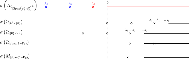
Figure 1: A representation of the spectrum of $\Omega$ and $M$ on ${\rm Ran}(1-P_{0})$ for $N=2$. The spectrum of $H[\rho_{0}]$ is represented on the first line, with the occupied eigenvalues in blue and the energies of the unoccupied states in red. The second and third lines represent the spectrum of $H[\rho_{0}]-\lambda_{i}$ $(i=1,2)$, i.e. the spectrum of $\Omega$ on each sector of the space. The circles correspond to eigenvectors in ${\rm Ran}(P_{0})$, the “hidden” excitations. The spectrum of $\Omega$ restricted to ${\rm Ran}(1-P_{0})$ is the combination of the shifted spectra, on the fourth line. The last line shows the spectrum of $M$ restricted to ${\rm Ran}(1-P_{0})$.

3 Main results

3.1 Well-posedness and linear response

Our first result is the well-posedness of (58) (and therefore of (4)):

Theorem 1 (Well-posedness of (58), linear response).

Under Assumptions 1 to 4, for any $T>0$, there exists $\varepsilon_{0}>0$ such that, for all $0<\varepsilon\leq\varepsilon_{0}$,

• The equation (58) admits a unique solution $U$ in $\mathcal{C}^{1}([0,T],(L^{2})^{2N})\cap\mathcal{C}^{0}([0,T],(H^{2})^{2N})$.

• We have

  $$\rho(t) =\rho_{\Psi^{0}(t)+\varepsilon U(t)}=\rho_{0}+\varepsilon\int_{0}^{t}\chi(t-t^{\prime})V_{P}f(t^{\prime})dt^{\prime}+\varepsilon^{2}r(t),$$ (65)

  with $\|r(t)\|_{H^{2}}\leq C_{T}$ for all $t\in[0,T]$ for some $C_{T}$ independent of $t$ and $\varepsilon$. The linear response function of the system $\chi(t)$, $t\in\mathbb{R}$ is a uniformly bounded operator from $H^{2}$ to $H^{2}$, and given by

  $$\boxed{\chi(t)V_{P}=-\theta(t)S_{0}\left(e^{-tJM}J(1-P_{0})V_{P}\Psi^{0}\right)}$$ (66)

  for all $V_{P}\in H^{2}$, with $\theta$ being the Heaviside function.

It also results from the estimates in the theorem that $\chi(t)$ defines a tempered distribution with values in ${\mathcal{L}}(H^{2},H^{2})$, with distributional time Fourier transform given by

$$\hat{\chi}(\omega)V_{P} =\lim_{\eta\rightarrow 0^{+}}-S_{0}\left(\frac{1}{M+{\rm i}(\omega+{\rm i}\eta)J}(1-P_{0})V_{P}\Psi^{0}\right).$$ (67)

The proof of this theorem is given in Section 4. It is based on a study of the linearized equation, using the coercivity result in Proposition 2 to define the exponential $e^{-tJM}$, as well as a fixed-point argument in the $H^{2}$ topology.

Remark 1 (Dyson equation in TDDFT).

To see the connection between (66) or (67) with the TDDFT equations in the Dyson formalism, one notices that the operator $\left\{\begin{aligned} H^{2}&\to(H^{2})^{2N}\\ V_{P}&\mapsto V_{P}\Psi_{0}\end{aligned}\right.$ is the $L^{2}$ adjoint of $S_{0}$. Hence $K_{0}(U)=S_{0}^{*}\Big{(}\frac{dv_{\mathrm{hxc}}}{d\rho}S_{0}(U)\Big{)}$. Thus in real time, introducing $P_{0}^{\perp}=1-P_{0}$, using a Duhamel formula on $P_{0}^{\perp}MP_{0}^{\perp}=P_{0}^{\perp}\Omega P_{0}^{\perp}+P_{0}^{\perp}KP_{0}^{\perp}$, we have

$$\chi(t)V_{P} =-\theta(t)S_{0}\left(\Big{(}e^{-tJP_{0}^{\perp}\Omega P_{0}^{\perp}}J-\int_{0}^{t}e^{-(t-s)JP_{0}^{\perp}\Omega P_{0}^{\perp}}JKe^{-sJP_{0}^{\perp}(\Omega+K)P_{0}^{\perp}}\,\mathrm{d}s\Big{)}JP_{0}^{\perp}V_{P}\Psi^{0}\right)$$ (68)

$$=\chi_{0}(t)V_{P}+S_{0}\left(\Big{(}\int_{\mathbb{R}}\theta(t-s)e^{-(t-s)JP_{0}^{\perp}\Omega P_{0}^{\perp}}JS_{0}^{*}\frac{dv_{\mathrm{hxc}}}{d\rho}S_{0}\theta(s)e^{-sJP_{0}^{\perp}(\Omega+K)P_{0}^{\perp}}\,\mathrm{d}s\Big{)}JP_{0}^{\perp}S_{0}^{*}V_{P}\right)$$ (69)

$$=\chi_{0}(t)V_{P}+\big{(}\chi_{0}\star\frac{dv_{\mathrm{hxc}}}{d\rho}\chi\big{)}(t)V_{P},$$ (70)

with $\chi_{0}(t)=-\theta(t)S_{0}\Big{(}e^{-tJP_{0}^{\perp}\Omega P_{0}^{\perp}}JP_{0}^{\perp}V_{P}\Psi_{0}\Big{)}$ which is the linear response function of the non-interacting evolution with $\Omega$ and $\star$ is the convolution in time.

3.2 Resonances

Our second result states that any eigenvalue embedded in the continuous spectrum of $\Omega$ turns into a resonance in the weakly interacting regime. We need the following extra assumptions:

Assumption 6 (Exponential decay of the total potential).

The operator of multiplication by the total potential

$$V_{\rm tot}=V_{\rm ext}+\left(\rho_{0}*\tfrac{1}{|r|}\right)+v_{\rm xc}(\rho_{0})$$ (71)

is bounded from $H^{2}_{\beta}$ to $L^{2}_{-\beta}$ for some $\beta>0$.

This assumption allows to analytically continue the resolvent beyond the real axis in the topology of exponentially localized functions. It is justified for atomic systems, where the rotational symmetry implies the exponential decay of $V_{\rm ext}+\left(\rho_{0}*\tfrac{1}{|r|}\right)$. It does not hold for general molecules, where the algebraic decay of the total potential is determined by the first non-zero moment of the total charge distribution. There, it might be possible to generalize it in two different directions. First, with less decay assumptions, we should be able to obtain a weaker notion of resonance [23]. Second, with minimal decay assumptions but assuming analyticity at infinity of $V_{\rm tot}$, it should be possible to obtain similar results as the ones in this paper [24] using the theory of analytic dilatations.

Assumption 7 (Excitation energy embedded in continuous spectrum).

Let $\lambda_{i_{0}}$ and $\lambda_{a_{0}}$ two eigenvalues of $H_{0}$, with ${i_{0}}\in\{1,...,N\}$ an occupied orbital and ${a_{0}}>N$ an unoccupied orbital (eigenvector of $H_{0}$). We assume

• $\lambda_{{a_{0}}}-\lambda_{{i_{0}}}>-\lambda_{N}$ (excitation embedded in continuous spectrum)

• $\lambda_{{a_{0}}}-\lambda_{{i_{0}}}\neq-\lambda_{i}$ for any $i=1,\dots,N$ (excitation not at ionization thresholds)

• $\lambda_{{a_{0}}}$ and $\lambda_{{i_{0}}}$ are simple eigenvalues.

The last assumption is not crucial, and is made to simplify the final expression of the decay rate.

Theorem 2.

Under Assumptions 1 to 7, there exists $\alpha_{0}>0$ such that, for all $0<\alpha<\alpha_{0}$, $\widehat{\chi}$ admits a meromorphic continuation as an operator from $(L^{2}_{\alpha})^{2N}$ to $(L^{2}_{-\alpha})^{2N}$ from the upper complex plane to a complex neighborhood of $\lambda_{{a_{0}}}-\lambda_{{i_{0}}}$.

If $\delta=\|K_{0}\|_{\mathcal{L}\left((L^{2}_{\alpha})^{2N},(H^{2}_{-\alpha})^{2N}\right)}$ is small enough and $\psi_{i_{0}}\overline{\psi}_{a_{0}}+\psi_{a_{0}}\overline{\psi}_{i_{0}}\not=0$, this continuation admits a single pole at a location $z_{\rm pole}$ with

$$\mathrm{Re}(z_{\rm pole})=\lambda_{a_{0}}-\lambda_{i_{0}}+\Delta E+O(\delta^{3}),\quad\text{and}\quad\mathrm{Im}(z_{\rm pole})=-\Gamma+O(\delta^{3}),$$ (72)

where $\Delta E$ and $\Gamma$, of second order in $\delta$, are given by a Fermi golden rule type expression (see (117)). In particular, $\Gamma$ is non-negative and generically non-zero.

This pole can be interpreted in several ways. In the linear response function $\widehat{\chi}(\omega)$ for $\omega$ real, it corresponds to a Breit-Wigner bump at frequency ${\rm Re}(z_{\rm pole})$ and with width $-{{\rm Im}(z_{\rm pole})}$; see for instance [7]. Dynamically, it corresponds to a long-lived state with lifetime $-\frac{1}{{\rm Im}(z_{\rm pole})}$; see for instance [20, 23].

4 Well-posedness and linear response

In this Section, we prove Theorem 1.

4.1 The linearized equation

We will do this by studying the linearized equation

$$J\partial_{t}U =M_{\rm dyn}U,\quad U(0)=U_{0}.$$ (73)

Lemma 1 (Well-posedness of the linearized equation).

Suppose that $e^{-JMt}$ defines a uniformly bounded semigroup in $(H^{2})^{2N}$, then for all $U_{0}\in(H^{2})^{2N}$, there exists a unique solution

$$U(t)=e^{-JM_{\rm dyn}t}U_{0}$$ (74)

of (73), satisfying

$$\|U(t)\|_{(H^{2})^{2N}}\leq C_{\rm dyn}(1+t^{2})\|U_{0}\|_{(H^{2})^{2N}}$$ (75)

for some $C_{\rm dyn}>0$ and for all $t\in\mathbb{R}$.

If furthermore $U_{0}\in{\rm Ran}(1-P_{0})$, then

$$\|U(t)\|_{(H^{2})^{2N}}\leq C\|U_{0}\|_{(H^{2})^{2N}}$$ (76)

for some $C>0$ and for all $t\in\mathbb{R}$.

Proof.

To prove this lemma, we look at the structure of orbital variations $U$. Any orbital variation $U\in Y_{\mathbb{R}}=(L^{2}(\mathbb{R}^{3},\mathbb{C})^{N},\mathbb{R})$ can be decomposed orthogonally as

$$U=U_{\rm S}+U_{\rm A}+U_{\perp},$$ (77)

where

$$U_{\rm S}=\Psi^{0}S,\quad U_{\rm A}=\Psi^{0}A,\quad U_{\perp}\in{\rm Ran}(1-P_{0})$$ (78)

with $S$ a $N\times N$ Hermitian matrix (explicitly: $S=S_{\rm r}+{\rm j}S_{\rm j}$ satisfies $S_{\rm r}^{T}=S_{\rm r},S_{\rm j}^{T}=-S_{\rm j}$) and $A$ a skew-Hermitian matrix. This corresponds to an orthogonal splitting of the space $Y_{\mathbb{R}}$ as

$$Y_{\mathbb{R}}=Y_{\mathbb{R},{\rm S}}+Y_{\mathbb{R},{\rm A}}+Y_{\mathbb{R},\perp}$$ (79)

which induces an orthogonal splitting of $Y=(L^{2})^{2N}$.

$$Y=Y_{\rm S}+Y_{\rm A}+Y_{\perp}.$$ (80)

The variations in $Y_{\rm S}$ are “growth modes”: they violate the normalization condition $\Psi^{*}\Psi=1$, whose tangent space is $Y_{\rm A}+Y_{\perp}$. This normalization condition is preserved by the flow of the nonlinear equation, and therefore its tangent space is preserved by the linearized equation:

$$(-JM_{\rm dyn}U)_{\rm S}=0\quad\forall U\in Y_{\rm A}+Y_{\perp}.$$ (81)

The variations in $Y_{\rm A}$ are “gauge modes”, that correspond to a rotation of the orbitals between themselves and therefore produce no observable physical output

$$S_{0}(U_{\rm A})=0\quad\forall U_{\rm A}\in Y_{\rm A},$$ (82)

so that in particular $K_{0}Y_{\rm A}=0$. By self-adjointness, ${\rm Ran}(K_{0})\perp Y_{\rm A}$. Finally, for any matrix $Q$

$$\Omega(\Psi^{0}Q)=\Psi^{0}Q^{\prime},\quad\text{ with }Q^{\prime}_{ij}=(\lambda_{i}-\lambda_{j})Q_{ij},$$ (83)

so that we have the following sparsity patterns:

$$J=\begin{pmatrix}0&J&0\\ J&0&0\\ 0&0&J\end{pmatrix},\quad\Omega=\begin{pmatrix}0&\ast&0\\ \ast&0&0\\ 0&0&\ast\end{pmatrix},\quad K_{0}=\begin{pmatrix}\ast&0&\ast\\ 0&0&0\\ \ast&0&\ast\end{pmatrix}.$$

Altogether, (73) can be rewritten as

$$\partial_{t}U =\begin{pmatrix}-J\Omega&0&0\\ L_{\rm AS}&-J\Omega&L_{A\perp}\\ L_{\rm\perp S}&0&-JM\end{pmatrix}U,$$ (84)

where $L_{\rm AS},L_{\rm A\perp}$ and $L_{\perp S}$ are blocks of $-JK_{0}$, whose expression is not relevant (they are bounded, since they have either a starting or ending space of finite dimension). The solution can therefore be obtained formally as

$$U_{\rm S}(t) =e^{-J\Omega t}U_{\rm S}(0)$$

$$U_{\perp}(t) =e^{-JMt}U_{\perp}(0)+\int_{0}^{t}e^{-JM(t-t^{\prime})}L_{\perp\rm S}U_{\rm S}(t^{\prime})dt^{\prime}$$

$$U_{\rm A}(t) =e^{Ct}U_{\rm A}(0)+\int_{0}^{t}e^{-J\Omega(t-t^{\prime})}(L_{\rm AS}U_{\rm S}(t^{\prime})+L_{\rm A\perp}U_{\perp}(t^{\prime}))dt^{\prime}$$

Since

$$J\Omega\stackrel{{\scriptstyle{\text{Casida}}}}{{\simeq}}\begin{pmatrix}{\rm i}\Omega&0\\ 0&-{\rm i}\Omega\end{pmatrix},$$

$e^{-J\Omega t}$ is unitary on the finite dimensional spaces $Y_{\rm S}$ and $Y_{\rm A}$ in the $L^{2}$ topology for all $t\in\mathbb{R}$, and therefore $e^{-J\Omega t}$ is bounded uniformly in time in the $H^{2}$ topology. Our task is therefore now to give a sense and obtain a uniform bound in time for $e^{-JMt}$ in the $H^{2}$ topology of $Y_{\perp}$, from which Lemma 1 follows immediately. ∎

The main difficulty to study $e^{-JMt}$ is that $-JM$ is not skew-adjoint because $J$ does not commute with $K_{0}$. This prevents us from using the self-adjoint functional calculus. However, since $M$ is positive, we can make use of the following formal equality

$$e^{-JMt}=M^{-1/2}e^{-M^{1/2}JM^{1/2}t}M^{1/2}$$

where now $M^{1/2}JM^{1/2}$ is skew-adjoint. Lemma 1 then follows from the following technical lemma:

Lemma 2 (Properties of $e^{-tM^{1/2}JM^{1/2}}$).

1. $x\mapsto\|Mx\|_{L^{2}}$ is an equivalent norm to $H^{2}$ on $\mathrm{Ran}(1-P_{0})$;

2. For any $t\in\mathbb{R}$, $e^{-tM^{1/2}JM^{1/2}}$ is unitary on $(L^{2})^{2N}$;

3. For $t\in\mathbb{R}$, $M^{-1/2}e^{-tM^{1/2}JM^{1/2}}M^{-1/2}$ as an operator on $(H^{2})^{2N}$ is uniformly bounded, i.e. there is a constant $C>0$ such that for all $t\in\mathbb{R}$

   $$\big{\|}M^{-1/2}e^{-tM^{1/2}JM^{1/2}}M^{1/2}\big{\|}_{\mathcal{L}\left((H^{2})^{2N},(H^{2})^{2N}\right)}\leq C;$$

4. For any $\Phi_{0}\in(H^{2})^{2N}$, let $\Phi(t)=M^{-1/2}e^{-tM^{1/2}JM^{1/2}}M^{1/2}\Phi_{0}$. Then $\Phi\in C^{0}(\mathbb{R},(H^{2})^{2N})\cap C^{1}(\mathbb{R},(L^{2})^{2N})$ solves $\Phi^{\prime}(t)=-JM\Phi(t)$.

Proof of Lemma 2.

1. $M$ induces a norm equivalent to the $H^{2}$ norm on ${\rm Ran}\left(1-P_{0}\right)$

   Let us first notice that $K_{0}$ is bounded from $(H^{2})^{2N}$ to itself. By Lemma 4, $X_{\perp}\mapsto\left(S_{0}(X_{\perp})*\frac{1}{|r|}\right)\Psi^{0}\in\mathcal{L}(H^{2},H^{2})$, and $v_{\rm xc}^{\prime}(\rho_{0})$ is bounded because $v_{\rm xc}^{\prime}$ is continuous.

   Let $X_{\perp}$ in $\big{(}H^{2}\big{)}^{2N}\cap{\rm Ran}\left(1-P_{0}\right)$.

   $$\|X_{\perp}\|_{H^{2}} =\|X_{\perp}\|_{L^{2}}+\|\Delta X_{\perp}\|_{L^{2}}$$ (85)

   $$\|MX_{\perp}\|_{L^{2}} =\|M(-\Delta+1)^{-1}(-\Delta+1)X_{\perp}\|_{L^{2}}$$ (86)

   $$\leq\|M(-\Delta+1)^{-1}\|_{\mathcal{L}\left((L^{2})^{2N},(L^{2})^{2N}\right)}\|X_{\perp}\|_{H^{2}}$$ (87)

   $(\Omega+K_{0})(-\Delta+1)^{-1}$ is bounded because $V_{\mathrm{tot}}+K_{0}$ is a $\Delta$-compact operator. Therefore the $H^{2}$ norm dominates $M$ on ${\rm Ran}\left(1-P_{0}\right)$. We now prove the reverse statement. We notice that $V_{\mathrm{tot}}+K_{0}$ is a $\Delta$-compact operator, thus $\Delta$-infinitesimally bounded:

   $$\forall\eta>0,\leavevmode\nobreak\ \exists C_{\eta}>0\leavevmode\nobreak\ :\leavevmode\nobreak\ \forall X_{\perp}\in\big{(}H^{2}\big{)}^{2N}\cap{\rm Ran}\left(1-P_{0}\right),$$ (88)

   $$\|(V_{\mathrm{tot}}+K_{0})X_{\perp}\|_{L^{2}} \leq\eta\|\Delta X_{\perp}\|_{L^{2}}+C_{\eta}\|X_{\perp}\|_{L^{2}}$$ (89)

   $$\|MX_{\perp}\|_{L^{2}} \geq\|(-\frac{1}{2}\Delta-\Lambda)X_{\perp}\|_{L^{2}}-\|(V_{\mathrm{tot}}+K_{0})X_{\perp}\|_{L^{2}}$$ (90)

   $$\|MX_{\perp}\|_{L^{2}} \geq(\tfrac{1}{2}-\eta)\|\Delta X_{\perp}\|_{L^{2}}-(C_{\eta}+\|\Lambda\|_{\mathcal{L}\left((L^{2})^{2N},(L^{2})^{2N}\right)})\|X_{\perp}\|_{L^{2}}$$ (91)

   Furthermore, $M$ is $L^{2}$-coercive:

   $$\exists c>0,\leavevmode\nobreak\ \forall X_{\perp}\in\big{(}H^{2}\big{)}^{2N}\cap{\rm Ran}\left(1-P_{0}\right),\leavevmode\nobreak\ \|MX_{\perp}\|_{L^{2}}\geq c\|X_{\perp}\|_{L^{2}}$$ (92)

   Combining equations (91)-(92) allows to conclude that $M$ dominates the $H^{2}$ norm on ${\rm Ran}\left(1-P_{0}\right)$. Thus the $M$ norm and the $H^{2}$ norm are equivalent on $\mathrm{Ran}(1-P_{0})$.

2. $e^{-M^{1/2}JM^{1/2}}$ is unitary on $\big{(}L^{2}\big{)}^{2N}$

   $M^{1/2}JM^{1/2}$ is a skew-adjoint operator on $\big{(}L^{2}\big{)}^{2N}$, with domain $\big{(}H^{2}\big{)}^{2N}$. We can exponentiate it, and:

   $$e^{-M^{1/2}JM^{1/2}}\in\mathcal{L}\left(\big{(}L^{2}\big{)}^{2N},\big{(}L^{2}\big{)}^{2N}\right)$$ (93)

   $e^{-M^{1/2}JM^{1/2}}$ is a unitary operator (and for any $t\in\mathbb{R}$, $e^{-tM^{1/2}JM^{1/2}}$ is unitary).

3. $M^{-1/2}e^{-tM^{1/2}JM^{1/2}}M^{1/2}$ is uniformly bounded in time from $\big{(}H^{2}\big{)}^{2N}$ to itself

   The proof is carried out in two steps. First we show that the $H^{1}$ norm is equivalent to the norm induced by $M^{1/2}$ on ${\rm Ran}\left(1-P_{0}\right)$. Let $X_{\perp}$ in $(H^{1})^{2N}\cap{\rm Ran}\left(1-P_{0}\right)$:

   $$\|M^{1/2}X_{\perp}\|_{L^{2}}^{2} =\langle X_{\perp},MX_{\perp}\rangle_{L^{2}}$$ (94)

   $$=\langle X_{\perp},(-\frac{1}{2}\Delta-\Lambda+V_{\mathrm{tot}}+K)X_{\perp}\rangle_{L^{2}}$$ (95)

   $$=\langle(-\frac{1}{2}\Delta-\Lambda)^{1/2}X_{\perp},(1+(-\frac{1}{2}\Delta-\Lambda)^{-1/2}(V_{\mathrm{tot}}+K)(-\frac{1}{2}\Delta-\Lambda)^{-1/2})(-\frac{1}{2}\Delta-\Lambda)^{1/2}X_{\perp}\rangle_{L^{2}}$$ (96)

   $$=\frac{1}{2}\langle\nabla X_{\perp},\nabla X_{\perp}\rangle_{L^{2}}+\langle X_{\perp},-\Lambda X_{\perp}\rangle_{L^{2}}$$ (97)

   $$\qquad\qquad+\langle(-\frac{1}{2}\Delta-\Lambda)^{1/2}X_{\perp},(-\frac{1}{2}\Delta-\Lambda)^{-1/2}(V_{\mathrm{tot}}+K)(-\frac{1}{2}\Delta-\Lambda)^{-1/2})(-\frac{1}{2}\Delta-\Lambda)^{1/2}X_{\perp}\rangle.$$ (98)

   Since $((-\frac{1}{2}\Delta-\Lambda)^{-1/2}(V_{\mathrm{tot}}+K)(-\frac{1}{2}\Delta-\Lambda)^{-1/2})^{2}$ is compact on $L^{2}$ and $(V_{\mathrm{tot}}+K)(-\frac{1}{2}\Delta-\Lambda)^{-1/2})^{2}$ is bounded from $(L^{2})^{2N}$ to $(L^{2})^{2N}$ by Lemma 6, then $(-\frac{1}{2}\Delta-\Lambda)^{-1/2}(V_{\mathrm{tot}}+K)(-\frac{1}{2}\Delta-\Lambda)^{-1/2}$ is compact on $L^{2}$. Thus, for any $\eta>0$, there is $C_{\eta}>0$, such that for all $U\in(L^{2})^{2N}\cap\mathrm{Ran}(1-P_{0})$

   $$\big{|}\langle U,(-\frac{1}{2}\Delta-\Lambda)^{-1/2}(V_{\mathrm{tot}}+K)(-\frac{1}{2}\Delta-\Lambda)^{-1/2})U\rangle_{L^{2}}\big{|}\leq\eta\langle U,U\rangle_{L^{2}}+C_{\eta}\langle(-\frac{1}{2}\Delta-\Lambda)^{-1/2}U,(-\frac{1}{2}\Delta-\Lambda)^{-1/2}U\rangle_{L^{2}}.$$

   Plugging in the previous equation, we have

   $$\|M^{1/2}X_{\perp}\|_{L^{2}}^{2}\leq\left(\frac{1}{2}-\eta\right)\Big{(}\langle\nabla X_{\perp},\nabla X_{\perp}\rangle_{L^{2}}+\langle X_{\perp},-\Lambda X_{\perp}\rangle_{L^{2}}\Big{)}-C_{\eta}\langle X_{\perp},X_{\perp}\rangle_{L^{2}}.$$

   Using this equation with $\eta$ small enough, and the $L^{2}$ coercivity of $M^{1/2}$, the same reasoning as before allows to conclude that $M^{1/2}$ is equivalent to the $H^{1}$ norm on ${\rm Ran}\left(1-P_{0}\right)$.

   We have seen that $M$ induces a norm equivalent to $H^{2}$ and $M^{1/2}$ to $H^{1}$. Since $J$ is unitary on $H^{1}$, $M^{1/2}JM^{1/2}$ induces a norm equivalent to the $H^{2}$ norm. Since it commutes with $e^{-tM^{1/2}JM^{1/2}}$, $e^{-tM^{1/2}JM^{1/2}}$ is a uniformly bounded operator from $(H^{2})^{2N}$ to $(H^{2})^{2N}$.

4. $M^{-1/2}e^{-M^{1/2}JM^{1/2}t}M^{1/2}$ is the semigroup associated to $\Phi^{\prime}=-JM\Phi$

   We first prove that $e^{-M^{1/2}JM^{1/2}t}$ is a bounded operator on $(H^{1})^{2N}$. Since $e^{-tM^{1/2}JM^{1/2}}$ is bounded as an operator on $L^{2}$ and $H^{2}$, by a Riesz-Thorin type interpolation argument [25, Theorems 7.1, 5.1], we have the $H^{1}$ bound

   $$\Big{\|}e^{-tM^{1/2}JM^{1/2}}\Big{\|}_{\mathcal{L}\left((H^{1})^{2N},(H^{1})^{2N}\right)}\leq\Big{\|}e^{-tM^{1/2}JM^{1/2}}\Big{\|}_{\mathcal{L}\left((L^{2})^{2N},(L^{2})^{2N}\right)}^{1/2}\Big{\|}e^{-tM^{1/2}JM^{1/2}}\Big{\|}_{\mathcal{L}\left((H^{2})^{2N},(H^{2})^{2N}\right)}^{1/2}.$$ (99)

   Now for $\Phi_{0}\in(H^{2})^{2N}$, let $\Phi(t)=M^{-1/2}e^{-M^{1/2}JM^{1/2}t}M^{1/2}\Phi_{0}$. Then

   $$\Phi^{\prime}(t)=-JMM^{-1/2}e^{-M^{1/2}JM^{1/2}t}M^{1/2}\Phi_{0}=-JM\Phi(t),$$

   where we have used that $M^{1/2}:(H^{1})^{2N}\to(L^{2})^{2N}$, $M^{-1/2}:(H^{1})^{2N}\to(H^{2})^{2N}$ are bounded on ${\rm Ran}(1-P_{0})$ and extended to ${\rm Ran}(P_{0})$ by the identify.

∎

4.2 Well-posedness of the nonlinear system

In this section, we prove that equation (58) is well-posed. By the Duhamel formula, any solution of (58) is also a solution of

$$U(t) =-\int_{0}^{t}e^{-JM_{\rm dyn}(t-t^{\prime})}J\left(f(t^{\prime})V_{P}\Psi^{0}+R(U,\varepsilon,t^{\prime})\right)dt^{\prime}.$$ (100)

Let

$$F(\varepsilon,U)(t)=U(t)+\int_{0}^{t}e^{-JM_{\rm dyn}(t-t^{\prime})}J\left(f(t^{\prime})V_{P}\Psi^{0}+R(U,\varepsilon,t^{\prime})\right)dt^{\prime}.$$ (101)

We solve the equation $F(\varepsilon,U)=0$ in the Banach space $\mathcal{C}^{0}\left([0,T],\big{(}H^{2}\big{)}^{2N}\right)$ for a fixed $T$. We first prove that $F$ is $\mathcal{C}^{1}$ on $\mathbb{R}\times\mathcal{C}^{0}([0,T],(H^{2})^{2N})$.

Recall that:

$${R}(U,\varepsilon,t) =\varepsilon f(t)V_{P}U+\epsilon^{-1}\left(H[\rho_{\Psi^{0}+\varepsilon U}]-H[\rho_{0}]\right)\Psi^{0}-K_{0}(U)+\left(H[\rho_{\Psi^{0}+\varepsilon U}]-H[\rho_{0}]\right)U$$ (102)

By assumption on $V_{P}$ and Lemma 6, $U\mapsto\epsilon f(t)V_{P}U-K_{0}(U)$ is linear and maps $(H^{2})^{2N}$ to itself. The mapping $\rho\mapsto H[\rho]-H[\rho_{0}]=v_{\rm hxc}(\rho)-v_{\rm hxc}(\rho_{0})$ is $\mathcal{C}^{1}$ from $L^{1}\cap H^{2}$ to $\mathcal{L}((H^{2})^{2N},(H^{2})^{2N})$ because of Assumption 2, and the density mapping $\Psi\mapsto\rho_{\Psi}$ is $\mathcal{C}^{\infty}$ from $(H^{2})^{2N}$ to $L^{1}\cap H^{2}$. This shows that $R$ is $\mathcal{C}^{1}$ in $U$ in the $(H^{2})^{2N}$ topology.

Since $e^{-JM_{\rm dyn}t}$ is bounded as an operator from $(H^{2})^{2N}$ to itself uniformly in $t\in[0,T]$, $F$ is $\mathcal{C}^{1}$ on $\mathbb{R}\times\mathcal{C}^{0}([0,T],(H^{2})^{2N})$.

Furthermore, $\|(H[\rho_{\Psi^{0}+\varepsilon U}]-H[\rho_{0}])\Psi^{0}-\varepsilon K_{0}(U)\|_{H^{2}}=O(\varepsilon^{2}\|U\|_{H^{2}}^{2})$ because $v_{xc}$ is $\mathcal{C}^{1}$. Thus $F(\varepsilon,U)(t)=U(t)+\int_{0}^{t}e^{-JM_{\rm dyn}(t-t^{\prime})}J\left(f(t^{\prime})V_{P}\Psi^{0}\right)dt^{\prime}+\mathcal{O}(\varepsilon\|U\|^{2}_{H^{2}})$. This shows that:

$$F(0,0) =0$$ (103)

$$\frac{\partial F}{\partial U}(0,0) ={\rm Id}$$ (104)

We can apply the implicit function theorem to $F$ on $\mathcal{C}^{0}\left([0,T],\big{(}H^{2}\big{)}^{2N}\right)$. For $\varepsilon$ small enough, there exists a unique solution $U(\varepsilon)$ of $F(\varepsilon,U)=0$ in a neighborhood of $0$. Finally, we can check that this solution is in $\mathcal{C}^{1}([0,T],(L^{2})^{2N})\cap\mathcal{C}^{0}([0,T],(H^{2})^{2N})$ and solves (58).

Again by the implicit function theorem, the solution $U(\varepsilon)$ is $\mathcal{C}^{1}$ from a neighborhood of $0$ to $\mathcal{C}^{0}\left([0,T],\big{(}H^{2}\big{)}^{2N}\right)$, and

$$\frac{d}{d\varepsilon}U(0)=-\frac{\partial F}{\partial U}(0,0)^{-1}\frac{\partial F}{\partial\varepsilon}(0,0)=-\int_{0}^{t}e^{-JM_{\rm dyn}(t-t^{\prime})}Jf(t^{\prime})V_{P}\Psi^{0}dt^{\prime}=U^{1}$$ (105)

It follows that, for all $t\in[0,T]$,

$$\rho(t)=\rho_{0}+\varepsilon\rho^{(1)}(t)+O(\varepsilon^{2})$$

in $H^{2}$, with $\rho^{(1)}(t)=S_{0}(U^{1}(t))$. Following the notations of section 4.1, $U^{1}_{S}=0$ and thus $S_{0}(U^{1}(t))=S_{0}(U^{1}_{\perp}(t))$. The expression of $U^{1}_{\perp}$ is given by:

$$U^{1}_{\perp}(t)=-\int_{0}^{t}e^{-JM(t-t^{\prime})}Jf(t^{\prime})V_{P}\Psi^{0}dt^{\prime}$$ (106)

The expression of $\chi(t)$ follows.

Since $t\mapsto U^{1}_{\perp}(t)$ is continuous and bounded in the $H^{2}$ topology, $\chi$ defines a tempered distribution on $\mathbb{R}$ with values in $\mathcal{L}(H^{2},H^{2})$. Since $\chi$ is causal, we have $\lim_{\eta\to 0^{+}}e^{-\eta t}\chi(t)=\chi(t)$ in the sense of tempered distributions. As operators on $H^{2}$, we have

$$\int_{0}^{\infty}e^{-\eta t}e^{i\omega t}e^{-JMt} =\frac{1}{JM-{\rm i}(\omega+{\rm i}\eta)}$$ (107)

so that, in the sense of tempered distributions,

$$\hat{\chi}(\omega)V_{P} =\lim_{\eta\rightarrow 0^{+}}-S_{0}\left(\frac{1}{JM-{\rm i}(\omega+{\rm i}\eta)}JV_{P}\psi^{0}\right)=\lim_{\eta\rightarrow 0^{+}}-S_{0}\left(\frac{1}{M+{\rm i}(\omega+{\rm i}\eta)J}V_{P}\psi^{0}\right).$$ (108)

5 Resonances

In this section, we prove Theorem 2 on resonances, assuming Assumptions 6 (exponential decay of the total potential) and 7 (non degenerate excitation energy $\lambda_{a}-\lambda_{i}$).

In the Casida representation,

$$M+{\rm i}zJ\stackrel{{\scriptstyle{\text{Casida}}}}{{\simeq}}\begin{pmatrix}\Omega-z&0\\ 0&\Omega+z\end{pmatrix}+K_{0}$$ (109)

where we recall that $(\Omega U)_{i}=\left(-\tfrac{1}{2}\Delta-\lambda_{i}\right)u_{i}+V_{\rm tot}u_{i}$. We will show the analytical continuation of the inverse of $M+{\rm i}zJ$ from the upper complex to the lower one by a perturbation argument, starting from the resolvent of the Laplacian. We will then study resonances by identifying an eigenvalue at the same energy as continuous spectrum in the operator $\Omega$, and proving that this generically becomes a resonance when perturbed by $K_{0}$.

5.1 Analytic continuation of the free Laplacian

We start with a classical lemma on the analytic continuation of the free Laplacian.

Lemma 3 (Meromorphic continuation of the resolvent of the free Laplacian).

For $\alpha>0$, the resolvent $(z+\tfrac{1}{2}\Delta)^{-1}$ as an operator from $L^{2}_{\alpha}$ to $H^{2}_{-\alpha}$ has an analytic continuation from the first quadrant ${\rm Re}(z)>0,{\rm Im}(z)>0$ to the region ${\rm Re}(z)>0,{\rm Im}(\sqrt{2z})>-\alpha$.

This lemma is classical and well-known in the mathematical study of resonances; see [26] for instance. Nevertheless, to keep the paper self-contained, we reprove it here.

Proof of Lemma 3.

Let $\varphi$ in $L^{2}_{\alpha}$ and $\psi$ in the dual space of $H^{2}_{-\alpha}$; in particular, $\psi\in H^{-2}$ and $\widehat{\psi}$ is smooth. We will study the analytic continuation in $z$ of $\langle\psi|(z+\tfrac{\Delta}{2})^{-1}\varphi\rangle$ as ${\rm Im}(z)$ becomes negative.

We use the usual Fourier transform convention in space, $\mathcal{F}\psi(q)=\tfrac{1}{(2\pi)^{3/2}}\int_{\mathbb{R}^{3}}e^{-{\rm i}q\cdot r}\psi(r)dr$. Then for ${\rm Im}(z)>0$, by the Parseval formula:

$$\langle\psi|(z+\tfrac{\Delta}{2})^{-1}|\varphi\rangle =\int_{\mathbb{R}^{3}}\frac{1}{z-\tfrac{1}{2}|q|^{2}}\overline{\mathcal{F}{\psi}(q)}\mathcal{F}{\varphi}(q)dq$$

Let $I\subset\mathbb{R}^{+}$ be an interval not touching $0$. We split the above integral in two contributions $A_{I}(z)$ and $A_{\mathbb{R}^{+}\setminus I}(z)$, according to whether $\tfrac{1}{2}|q|^{2}$ belongs to $I$ or not.

For $A_{\mathbb{R}^{+}\setminus I}(z)$, since $\psi\in H^{-2}$ and $\phi\in L^{2}$, we have that

$$A_{\mathbb{R}^{+}\setminus I}(z) =\int_{q\in\mathbb{R}^{3},\tfrac{1}{2}|q|^{2}\notin I}\frac{1}{z-\tfrac{1}{2}|q|^{2}}\overline{\mathcal{F}{\psi}(q)}\mathcal{F}{\varphi}(q)dq$$

$$=\int_{q\in\mathbb{R}^{3},\tfrac{1}{2}|q|^{2}\notin I}\frac{1+|q|^{2}}{z-\tfrac{1}{2}|q|^{2}}\frac{\overline{\mathcal{F}{\psi}(q)}}{1+|q|^{2}}\mathcal{F}{\varphi}(q)dq$$

is analytic for $z$ in $I+{\rm i}\mathbb{R}$.

We now write $A_{I}(z)$ as

$$A_{I}(z) =\int_{I}\frac{1}{z-\lambda}\underbrace{\frac{1}{(2\pi)^{3}}\int_{S^{2}}{\overline{\mathcal{F}{\psi}(\sqrt{2\lambda}\tilde{q})}\mathcal{F}{\varphi}(\sqrt{2\lambda}\tilde{q})}\sqrt{2\lambda}d\tilde{q}}_{f(\lambda)}d\lambda.$$

The functions defined for $\lambda$ real by

$$\mathcal{F}\varphi(\sqrt{2\lambda}\tilde{q}) =\int_{\mathbb{R}^{3}}e^{-{\rm i}\sqrt{2\lambda}\tilde{q}r}\varphi(r)dr=\int_{\mathbb{R}^{3}}e^{-{\rm i}{\rm Re}(\sqrt{2\lambda})\tilde{q}r}e^{{{\rm Im}(\sqrt{2\lambda})\tilde{q}r}}\varphi(r)dr$$

$${\overline{\mathcal{F}\psi\left({\sqrt{2\lambda}}\tilde{q}\right)}} =\int_{\mathbb{R}^{3}}e^{{\rm i}\sqrt{2\lambda}\tilde{q}r}\overline{\psi(r)}dr=\int_{\mathbb{R}^{3}}e^{{\rm i}{\rm Re}(\sqrt{2\lambda})\tilde{q}r}e^{-{{\rm Im}(\sqrt{2\lambda})\tilde{q}r}}\overline{\psi(r)}dr$$

(where the second line is to be understood in the sense of distributions) extend analytically for $\lambda$ in the set

$$D_{I,\alpha}=\{z\in I+{\rm i}\mathbb{R},|{\rm Im}(\sqrt{2z})|<\alpha\}.$$

It follows that $f$ also extends to this set, so that, for $z\in D_{I,\alpha},{\rm Im}(z)>0$

$$A_{I}(z) =\int_{I}\frac{1}{z-\lambda}f(\lambda)d\lambda=\int_{C_{\varepsilon}}\frac{1}{z-\lambda}f(\lambda)d\lambda$$

where $C_{\varepsilon}$ is a contour starting at $\inf I$, dropping vertically to the bottom of $D_{I,\alpha-\varepsilon}$, following its lower edge, and coming back up at $\sup I$. This shows that $A_{I}$ extends analytically to $D_{I,\alpha-\varepsilon}$. Since $I$ and $\varepsilon$ were arbitrary, this concludes the proof.

∎

5.2 Meromorphic continuation of the resolvent of $JM$

Consider the family of operators defined in the Casida representation by

$$-\tfrac{1}{2}\Delta-\Lambda+{\rm i}zJ\stackrel{{\scriptstyle{\text{Casida}}}}{{\simeq}}\begin{pmatrix}-\tfrac{1}{2}\Delta-\Lambda-z&0\\ 0&-\tfrac{1}{2}\Delta-\Lambda+z\end{pmatrix}$$ (110)

From Assumption 7, when $z$ is close to $\lambda_{a_{0}}-\lambda_{i_{0}}$, the shifts $(\lambda_{i}\pm z)$ are close to a nonzero real number. It follows from the previous Lemma that this family has an inverse that can be continued analytically from the upper half complex plane to a complex neighborhood of $\lambda_{a_{0}}-\lambda_{i_{0}}$ as an operator from $L^{2}_{\alpha}$ to $H^{2}_{-\alpha}$. We now write formally for ${\rm Im}(z)>0$

$$M_{\mathrm{dyn}}+{\rm i}zJ =-\tfrac{1}{2}\Delta-\Lambda+{\rm i}zJ+(V_{\rm tot}+K_{0})$$ (111)

$$\frac{1}{M_{\mathrm{dyn}}+{\rm i}zJ} =\frac{1}{-\tfrac{1}{2}\Delta-\Lambda+{\rm i}zJ}\left(1+(V_{\rm tot}+K_{0})\frac{1}{-\tfrac{1}{2}\Delta-\Lambda+{\rm i}zJ}\right)^{-1}.$$ (112)

This formal computation is justified in the proof of Proposition 4

Proposition 4 (Meromorphic continuation of $(M+{\rm i}zJ)^{-1}$).

For $\alpha>0$ small enough, the operator $(M+{\rm i}zJ)^{-1}$ from $(L^{2}_{\alpha})^{2N}$ to $(H^{2}_{\alpha})^{2N}$ has an analytic continuation from the upper complex plane to a complex neighborhood of $\lambda_{a_{0}}-\lambda_{i_{0}}$.

Proof.

We have for all $\omega\in\mathbb{R},\eta>0$

$$\left\|(V_{\rm tot}+K_{0})\frac{1}{-\tfrac{1}{2}\Delta-\Lambda+{\rm i}(\omega+{\rm i}\eta)J}\right\|_{L^{2}_{\alpha}\to L^{2}_{\alpha}} \leq\|V_{\rm tot}+K_{0}\|_{H^{2}_{-\alpha}\to L^{2}_{\alpha}}\|(-\tfrac{1}{2}\Delta-\Lambda\pm(\omega+i\eta))^{-1}\|_{L^{2}_{\alpha}\to H^{2}_{-\alpha}}$$

$$\leq\|V_{\rm tot}+K_{0}\|_{H^{2}_{-\alpha}\to L^{2}_{\alpha}}\|(-\tfrac{1}{2}\Delta-\Lambda\pm(\omega+i\eta))^{-1}\|_{L^{2}\to H^{2}}$$

$$\leq\frac{1}{\eta}\|V_{\rm tot}+K_{0}\|_{H^{2}_{-\alpha}\to L^{2}_{\alpha}}$$

so that $1+(V_{\rm tot}+K_{0})(-\tfrac{1}{2}\Delta-\Lambda+{\rm i}(\omega+{\rm i}\eta)J)^{-1}$ is invertible for $\eta$ large enough in $L^{2}_{\alpha}$. It follows from the analytic Fredholm theorem (Theorem C.8 of [20]) that $1+(V_{\rm tot}+K_{0})(-\tfrac{1}{2}\Delta-\Lambda+{\rm i}(\omega+{\rm i}\eta)J)^{-1}$ has a meromorphic continuation to a complex neighborhood of $\lambda_{a_{0}}-\lambda_{i_{0}}$, and the result follows by (112). ∎

This proves the first part of Theorem 2.

5.3 Resonances

We now prove the second part of Theorem 2. We now investigate the poles of $(M_{\mathrm{dyn}}+{\rm i}zJ)^{-1}$ on ${\rm Ran}(1-P_{0})$, which are also the poles of $(M+{\rm i}zJ)^{-1}$, in the asymptotic regime where $K_{0}$ is small.

For $K_{0}=0$, in the Casida representation,

$$\Omega+{\rm i}zJ\stackrel{{\scriptstyle{\text{Casida}}}}{{\simeq}}\begin{pmatrix}\Omega-z&0\\ 0&\Omega+z\end{pmatrix}$$ (113)

Near $z=\lambda_{a_{0}}-\lambda_{i_{0}}>0$, the block $\Omega+z$ is always invertible for ${\rm Im}(z)>0$. The operator $\Omega+{\rm i}(\lambda_{a_{0}}-\lambda_{i_{0}})J$ has a simple zero eigenvalue with eigenvector

$$(U_{i_{0}\to a_{0}})_{i}\stackrel{{\scriptstyle{\text{Casida}}}}{{\simeq}}\delta_{i,i_{0}}\begin{pmatrix}\psi_{a_{0}}\\ 0\end{pmatrix}$$ (114)

where $H_{0}\psi_{a_{0}}=\lambda_{a_{0}}\psi_{a_{0}}$ with $\|\psi_{a_{0}}\|=1$. It also has continuous spectrum at $0$ in all the ionized sectors $i$ such that $\lambda_{a_{0}}-\lambda_{i_{0}}>-\lambda_{i}$. By the results of the previous section, the inverse of its analytic continuation from $L^{2}_{\alpha}$ to $H^{2}_{-\alpha}$ has a single pole at $\lambda_{a_{0}}-\lambda_{i_{0}}$, with residue $P_{i_{0}\to a_{0}}=|U_{i_{0}\to a_{0}}\rangle\langle U_{i_{0}\to a_{0}}|$.

We now split the space $(L^{2})^{2N}$ orthogonally in ${\rm Ran}(P_{i_{0}\to a_{0}})$ and ${\rm Ran}(1-P_{i_{0}\to a_{0}})$. By a perturbation argument, there exists a complex neighborhood of $\lambda_{a_{0}}-\lambda_{i_{0}}$ inside which, for $\delta=\|K_{0}\|_{L^{2}_{\alpha}\to H^{2}_{-\alpha}}$ small enough, the orthogonal restriction on ${\rm Ran}(1-P_{i_{0}\to a_{0}})$ of the operator $M+{\rm i}zJ$ is invertible; let

$$R^{\perp}(z)=\left((M+{\rm i}zJ)|_{{\rm Ran}(1-P_{i_{0}\to a_{0}})}\right)^{-1}$$

this inverse. By a Schur complement, the operator $M+{\rm i}zJ$ is not invertible as an operator from $L^{2}_{-\alpha}$ to $L^{2}_{\alpha}$ if and only if the scalar Schur complement $S(z)$ vanishes, where

$$S(z) =\langle U_{i_{0}\to a_{0}}|M+{\rm i}zJ|U_{i_{0}\to a_{0}}\rangle-\langle U_{i_{0}\to a_{0}}|(M+{\rm i}zJ)R^{\perp}(z)(M+{\rm i}zJ)|U_{i_{0}\to a_{0}}\rangle$$ (115)

$$=(\lambda_{a_{0}}-\lambda_{i_{0}}-z)+\langle U_{i_{0}\to a_{0}}|K_{0}|U_{i_{0}\to a_{0}}\rangle-\langle U_{i_{0}\to a_{0}}|(M+{\rm i}zJ)R^{\perp}(z)(M+{\rm i}zJ)|U_{i_{0}\to a_{0}}\rangle.$$ (116)

This is an analytic equation in $z$, and the third term is of order $2$ in $\delta$ for $z$ in a small enough neighborhood of $\lambda_{a_{0}}-\lambda_{i_{0}}$. It follows by the implicit function theorem that, for $\delta$ small enough, there is a zero $z_{\rm pole}$ of $S$ close to $\lambda_{a_{0}}-\lambda_{i_{0}}$ such that

$$z_{\rm pole}=\lambda_{a_{0}}-\lambda_{i_{0}}+\langle U_{i_{0}\to a_{0}}|K_{0}|U_{i_{0}\to a_{0}}\rangle-\lim_{\eta\to 0^{+}}\langle U_{i_{0}\to a_{0}}|K_{0}R^{\perp}(\lambda_{a_{0}}-\lambda_{i_{0}}+{\rm i}\eta)K_{0}|U_{i_{0}\to a_{0}}\rangle+O(\delta^{3}).$$ (117)

By the Sokhotski-Plemelj formula, the skew-adjoint part of $\lim_{\eta\to 0^{+}}R^{\perp}(\lambda_{a_{0}}-\lambda_{i_{0}}+{\rm i}\eta)$ is given by

$$\lim_{\eta\to 0^{+}}{\mathcal{A}}(R^{\perp}(\lambda_{a_{0}}-\lambda_{i_{0}}+{\rm i}\eta))\stackrel{{\scriptstyle{\text{Casida}}}}{{\simeq}}{\rm i}\pi\sum_{\begin{subarray}{c}1\leq i\leq N\\ \lambda_{a_{0}}-\lambda_{a_{0}}+\lambda_{i}>0\end{subarray}}(\Pi_{i}^{+})^{*}p_{H_{0}}(\lambda_{a_{0}}-\lambda_{i_{0}}+\lambda_{i})\Pi_{i}^{+}$$ (118)

where $p_{H_{0}}(\lambda)d\lambda$ is the projection-valued measure associated with $H_{0}$ and

$$(\Pi_{i}^{+}U)_{j}\stackrel{{\scriptstyle{\text{Casida}}}}{{\simeq}}\delta_{ij}\begin{pmatrix}u_{j}\\ 0\end{pmatrix}$$

is the projection on the upper block, $i$-th sector of $(L^{2})^{2N}$.

It follows that

$${\rm Im}(z_{\rm pole})=-\pi\sum_{i,\lambda_{a_{0}}-\lambda_{a_{0}}+\lambda_{i}>0}\langle U_{i_{0}\to a_{0}}|K_{0}(\Pi_{i}^{+})^{*}p_{H_{0}}(\lambda_{a_{0}}-\lambda_{i_{0}}+\lambda_{i})\Pi_{i}^{+}K_{0}|U_{i_{0}\to a_{0}}\rangle+O(\delta^{3}).$$ (119)

It remains to check that the residue at this pole is nonzero. By definition of $\chi$, it is the case if $\langle S_{0}^{*}V_{P},U_{i_{0}\to a_{0}}\rangle\not=0$ for some $V_{P}\in H^{2}$, i.e. $S_{0}U_{i_{0}\to a_{0}}=\psi_{i_{0}}\overline{\psi}_{a_{0}}+\psi_{a_{0}}\overline{\psi}_{i_{0}}\not=0$.

Appendices

Appendix A Second-order expansion of the energy

Proof of Proposition 1.

The energy is

$$\mathcal{E}(\Psi) =\sum_{i=1}^{N}\left(\frac{1}{2}\int_{\mathbb{R}^{3}}|\nabla\psi_{i}(r)|^{2}+\int_{\mathbb{R}^{3}}V_{\rm ext}(r)|\psi_{i}(r)|^{2}dr\right)+\frac{1}{2}\int_{\mathbb{R}^{3}}\frac{\rho_{\Psi}(r)\rho_{\Psi}(r^{\prime})}{|r-r^{\prime}|}drdr^{\prime}+\int_{\mathbb{R}^{3}}e_{\rm xc}(\rho_{\Psi}(r))dr$$ (120)

We treat these terms in order. The first term is clearly smooth from $H^{2}$ to $\mathbb{R}$. Since $H^{2}$ is an algebra, the mapping $\psi_{i}\mapsto|\psi_{i}|^{2}$ is smooth from $H^{2}$ to $H^{2}$, and so by

$$\left|\int_{\mathbb{R}^{3}}(V_{1}+V_{2})|\psi_{i}|^{2}\right|\leq\|V_{1}\|_{L^{2}}\||\psi_{i}|^{2}\|_{L^{2}}+\|V_{2}\|_{L^{\infty}}\|\psi_{i}\|_{L^{2}}^{2},$$ (121)

the second term is also smooth from $H^{2}$ to $\mathbb{R}$. From Lemma 4, the map from $\Psi$ to the operator $L_{\Psi}$ of multiplication by $\rho_{\Psi}\ast\frac{1}{|r|}$ is smooth from $H^{2}$ to $\mathcal{L}(H^{2},H^{2})$, and therefore the third term

$$\frac{1}{2}\int_{\mathbb{R}^{3}}\frac{\rho_{\Psi}(r)\rho_{\Psi}(r^{\prime})}{|r-r^{\prime}|}drdr^{\prime}=\frac{1}{2}\sum_{i=1}^{N}\langle\psi_{i}|L_{\Psi}\psi_{i}\rangle$$ (122)

is smooth from $H^{2}$ to $\mathbb{R}$.

For all $\Psi\in(H^{2})^{N}$, $\Psi$ is bounded so $\rho$ is also bounded. Since $e_{\rm xc}(0)=0$, there is $C_{\Psi}$ such that $|e_{\rm xc}(\rho)|\leq C_{\Psi}\rho$. Since $\rho$ is integrable, so is $e_{\rm xc}(\rho)$. Furthermore, since $e_{\rm xc}$ is $\mathcal{C}^{2}$:

$$e_{\rm xc}(\rho) =e_{xc}(0)+\rho e_{\rm xc}^{\prime}(0)+\frac{\rho^{2}}{2}e_{xc}^{\prime\prime}(0)+o(\rho^{2})$$ (123)

Since $e_{\rm xc}(0)=0$ and $\rho$ as well as $\rho^{2}$ are integrable for $\rho\in H^{2}$, $\Psi\mapsto\int_{\mathbb{R}^{3}}e_{xc}(\rho_{\Psi}(r))dr$ is $\mathcal{C}^{2}$ from $H^{2}$ to $\mathbb{R}$. ∎

Proof of Proposition 2.

Let $U^{1}\in(H^{2})^{2N}\cap{\rm Ran}(1-P_{0})$. For all $\varepsilon>0$, let

$$\Psi(\varepsilon)={\rm Ortho}(\Psi^{0}+\varepsilon U^{1}),$$

where

$${\rm Ortho}(\Psi)=\Psi(\Psi^{*}\Psi)^{-1/2}.$$

We have the expansion

$$\Psi(\varepsilon)=\Psi^{0}+\varepsilon U^{1}+\varepsilon^{2}U^{2}+O(\varepsilon^{3})$$

in $H^{2}$.

Since $\Psi(\varepsilon)^{*}\Psi(\varepsilon)=1$ for all $\varepsilon$, by identification, we get

$$(U^{2})^{*}U^{0}+(U^{0})^{*}U^{2}=-(U^{1})^{*}U^{1}.$$ (124)

We can then compute

$$\mathcal{E}(\Psi(\varepsilon)) =\mathcal{E}(\Psi^{0})+2{\rm Re}\langle H_{0}\Psi^{0}|\varepsilon U^{1}+\varepsilon^{2}U^{2}\rangle+\langle\varepsilon U^{1}|H_{0}|\varepsilon U^{1}\rangle+{\rm Re}\langle\varepsilon U^{1}|\mathcal{K}_{0}(\varepsilon U^{1})\rangle+o(\varepsilon^{2})$$

$$=\mathcal{E}(\Psi^{0})+\varepsilon^{2}\Big{(}2{\rm Re}\langle H_{0}\Psi^{0}|U^{2}\rangle+\langle U^{1}|H_{0}|U^{1}\rangle+{\rm Re}\langle U^{1}|\mathcal{K}_{0}(U^{1})\rangle\Big{)}+o(\varepsilon^{2})$$

$$2{\rm Re}\langle H_{0}\Psi^{0}|U^{2}\rangle =2{\rm Re}\left(\sum_{i=1}^{N}\lambda_{i}\langle\psi^{0}_{i}|u_{i}^{2}\rangle\right)$$

$$=-\sum_{i=1}^{N}\lambda_{i}\langle u_{i}^{1}|u_{i}^{1}\rangle\mbox{ by \eqref{eq:critere_2_manifold}}$$

so that

$$\mathcal{E}(\Psi(\varepsilon)) =\mathcal{E}(\Psi^{0})+\varepsilon^{2}\langle U^{1}|\mathcal{M}_{\rm dyn}(U^{1})\rangle+o(\varepsilon^{2}).$$ (125)

On the other hand, we can solve the orthogonal Procustes problem

$$\min_{R\in{\rm U}(N)}\|\Psi-\Psi^{0}R\|^{2} =2N-2\max_{R\in{\rm U}(N)}{\rm Re}\langle\Psi,\Psi^{0}R\rangle$$

$$=2N-2\max_{R\in{\rm U}(N)}{\rm Re}\langle(\Psi^{0})^{*}\Psi,R\rangle$$

$$=2N-2\max_{R\in{\rm U}(N)}{\rm Re}\langle(\Psi^{0})^{*}\Psi,R\rangle$$

$$=2N-2\max_{R^{\prime}\in{\rm U}(N)}{\rm Re}\langle\Sigma,R^{\prime}\rangle$$

$$=2N-2{\rm Tr}(\Sigma)$$

where $\Sigma$ is the diagonal matrix of the singular values of $(\Psi^{0})^{*}\Psi$. We have

$$(\Psi^{0})^{*}\Psi =1+\varepsilon^{2}(U^{0})^{*}U^{2}+O(\varepsilon^{3})$$

$$((\Psi^{0})^{*}\Psi)^{*}((\Psi^{0})^{*}\Psi) =1+\varepsilon^{2}\left((U^{0})^{*}U^{2}+(U^{0})^{*}U^{2}\right)+O(\varepsilon^{3})$$

$$=1+2\varepsilon^{2}(U^{1})^{*}U^{1}+O(\varepsilon^{3})$$

$${\rm Tr}(\Sigma) ={\rm Tr}\left(\sqrt{((\Psi^{0})^{*}\Psi)^{*}((\Psi^{0})^{*}\Psi)}\right)$$

$$=N+\varepsilon^{2}{\rm Tr}\left((U^{1})^{*}U^{1}\right)+O(\varepsilon^{3})$$

so that

$$\min_{R\in{\rm U}(N)}\|\Psi-\Psi^{0}R\|^{2} =2\varepsilon^{2}\|U^{1}\|^{2}+O(\varepsilon^{3})$$

and the result follows.

∎

Appendix B Control of the Coulomb terms

We state a useful technical lemma, which ensures stability in $H^{2}$ in several occasions through the article.

Lemma 4.

Let $f$, $g$, $h$ three functions of $H^{2}$. Then the function $(fg*\tfrac{1}{|r|})h$ is in $H^{2}$, and there exists a constant $c$ such that:

$$\|(fg*\tfrac{1}{|r|})h\|_{H^{2}}\leq c\|f\|_{H^{2}}\|g\|_{H^{2}}\|h\|_{H^{2}}.$$ (126)

The proof relies on the Hardy-Littlewood-Sobolev (HLS) inequality in dimension 3:

$$\forall p,q>0;\leavevmode\nobreak\ 1<p,q<\infty,\leavevmode\nobreak\ s.t.\leavevmode\nobreak\ 1+\frac{1}{p}=\frac{1}{q}+\frac{1}{3},$$ (127)

$$\exists C_{HLS}^{p,q}>0,\leavevmode\nobreak\ \forall a\in L^{q}:\leavevmode\nobreak\ a*\tfrac{1}{|r|}\in L^{p}\mbox{ and }\|a*\frac{1}{|r|}\|_{L^{p}}\leq C_{HLS}^{p,q}\|a\|_{L^{q}}.$$ (128)

Lemma 5.

Let $a$ and $b$ two complex valued functions such that $a$ is in $L^{1}\cap L^{\tfrac{3}{2}}$ and $b$ is in $L^{t}$, with $t$ in $(2,6)$. Then $(a*\tfrac{1}{|r|})b$ is $L^{2}$, and $\|(a*\tfrac{1}{|r|})b\|_{L^{2}}\leq c(\|a\|_{L^{1}}+\|a\|_{L^{\frac{3}{2}}})\|b\|_{L^{t}}$, where $c$ is an unimportant constant.

Proof of Lemma 5.

Let $p$ such that $\frac{1}{p}+\frac{1}{t}=\frac{1}{2}$, with $t$ in $(2,6)$. Then $p$ is in $(3,+\infty)$. Thus there exists $q$ in $(1,\frac{3}{2})$ such that $p$ and $q$ are an admissible pair for the HLS inequality. Since $a$ is in $L^{1}\cap L^{\tfrac{3}{2}}$, it is in $L^{q}$ as well and we can write:

$$\|a*\frac{1}{|r|}\|_{L^{p}}\leq C_{HLS}^{p,q}\|a\|_{L^{q}}$$ (129)

By the Hölder inequality, $(a*\frac{1}{|r|})b$ is $L^{2}$ and:

$$\|\left(a*\frac{1}{|r|}\right)b\|_{L^{2}} \leq C_{HLS}^{p,q}\|a\|_{L^{q}}\|b\|_{L^{t}}$$ (130)

$$\|\left(a*\frac{1}{|r|}\right)b\|_{L^{2}} \leq C_{HLS}^{p,q}(\|a\|_{L^{1}}+\|a\|_{L^{\frac{3}{2}}})\|b\|_{L^{t}}$$ (131)

∎

Figure 2: Choices of $p$, $q$, $t$ to apply Lemma 5

Proof of Lemma 4.

We prove that $\left(fg*\tfrac{1}{|r|}\right)h$ is $L^{2}$ and then that its second derivative is $L^{2}$ as well. The proof is the application of Lemma 5.

$fg$ is in $H^{2}$, it thus belongs to $L^{\infty}\cap L^{2}$. It is $L^{1}$ as well by the Hölder inequality, since both $f$ and $g$ are $L^{2}$. Therefore $fg$ is $L^{1}\cap L^{\tfrac{3}{2}}$. $h$ is $L^{2}\cap L^{\infty}$, in particular it is $L^{t}$ for any $t$ in $(2,6)$, and we can apply Lemma 5.

We now show that the second derivative of the function belongs to $L^{2}$ . It only contains terms of the following form:

• $\left(f\nabla^{2}g*\tfrac{1}{|r|}\right)h$. $f$ and $\nabla^{2}g$ are both $L^{2}$, thus their product is $L^{1}$. Since $f$ is bounded and $\nabla^{2}g$ is $L^{2}$, $f\nabla^{2}g$ is $L^{2}$ as well and Lemma 5 can be applied.

• $\left(\nabla f\nabla g*\tfrac{1}{|r|}\right)h$. $\nabla f$ and $\nabla g$ are both $L^{2}$, thus their product is $L^{1}$. They are also both in $H^{1}$, which injects itself continuously (by Sobolev injection) in $L^{6}$ in dimension 3. Their product is thus in $L^{3}$.

• $\left(f\nabla g*\tfrac{1}{|r|}\right)\nabla h$. $f\nabla g$ is $L^{1}\cap L^{2}$. $\nabla h$ belongs to $H^{1}$, which injects itself continuously in $L^{6}$ by the Sobolev inequality. It also belongs to $L^{2}$.

• $\left(fg*\tfrac{1}{|r|}\right)\nabla^{2}h$. In this case, the HLS inequality cannot be directly applied, since $h$ is only $L^{2}$. We would need $\left(fg*\tfrac{1}{|r|}\right)$ to be $L^{\infty}$ for the Hölder inequality, which is not an admissible $p$ exponent. However, boundedness can easily be obtained like this:

  $$\forall r\in\mathbb{R}^{3},|\left(fg*\tfrac{1}{|r|}\right)(r)| \leq\int_{\mathbb{R}^{3}}\frac{|(fg)(r^{\prime})|}{|r-r^{\prime}|}dr^{\prime}$$ (132)

  $$=\int_{\mathcal{B}_{r,1}}\frac{|(fg)(r^{\prime})|}{|r-r^{\prime}|}dr^{\prime}+\int_{\mathbb{R}^{3}\backslash\mathcal{B}_{r,1}}\frac{|(fg)(r^{\prime})|}{|r-r^{\prime}|}dr^{\prime}$$ (133)

  $$\leq\int_{\mathcal{B}_{0,1}}\frac{1}{|r^{\prime}|}dr^{\prime}\sup_{r^{\prime}\in\mathbb{R}^{3}}|(fg)(r^{\prime})|+\int_{\mathbb{R}^{3}}|(fg)(r^{\prime})|dr^{\prime}$$ (134)

  $$\leq K\|f\|_{L^{\infty}}\|g\|_{L^{\infty}}+\|f\|_{L^{2}}\|g\|_{L^{2}}\quad\mbox{with}\quad K=\int_{\mathcal{B}_{0,1}}\frac{1}{|r^{\prime}|}dr^{\prime}.$$ (135)

∎

Appendix C Technical lemmas on $S_{0}$ and $K_{0}$

Lemma 6.

The following assertions are true:

1. $S_{0}:(H^{2})^{2N}\to(H^{2})^{2}$ is bounded;

2. $K_{0}:(H^{1})^{2N}\to(L^{2})^{2N}$ is bounded;

3. $K_{0}:(H^{2})^{2N}\to(H^{2})^{2N}$ is bounded;

4. $K_{0}:(H^{2})^{2N}\to(L^{2})^{2N}$ is compact;

5. For $\alpha>0$ small enough, $K_{0}:(H_{\alpha}^{2})^{2N}\to(L_{-\alpha}^{2})^{2N}$ is bounded.

Proof.

1. $S_{0}:(H^{2})^{2N}\to(H^{2})^{2}$ is bounded

   This follows from Assumption 3 and the fact that $H^{2}$ is an algebra.

2. $K_{0}:(H^{1})^{2N}\to(L^{2})^{2N}$ is bounded

   Again by Assumption 3, for $U\in(H^{1})^{2N}$, $S_{0}(U)\in(H^{1})^{2N}$, so by assumption on $v_{\mathrm{xc}}$, $v^{\prime}_{\mathrm{xc}}(\rho_{0})S_{0}(U)\Psi_{0}\in(H^{1})^{2N}$. For $S_{0}(U)*\frac{1}{|r|}$, we use a Hardy inequality to deduce that $\|S_{0}(U)*\frac{1}{|r|}\|_{L^{2}}\leq\|U\|_{H^{1}}$. This proves the assertion.

3. $K_{0}:(H^{2})^{2N}\to(H^{2})^{2N}$ is bounded

   By assumption on $v_{\mathrm{xc}}$, and since $H^{2}$ is an algebra, for $U\in(H^{2})^{2N}$, $v^{\prime}_{\mathrm{xc}}(\rho_{0})S_{0}(U)\Psi_{0}\in(H^{2})^{2N}$. By Lemma 4, we have that $S_{0}(U)*\frac{1}{|r|}\Psi_{0}\in(H^{2})^{2N}$ for $U\in(H^{2})^{2N}$. This finishes the proof of this item.

4. $K_{0}:(H^{2})^{2N}\to(L^{2})^{2N}$ is compact

   For the proof of the compactness of $K_{0}$, we have for $U\in(H^{2})^{2N}$

   $$K_{0}(U)=\big{(}S_{0}(U)*\frac{1}{|\cdot|}+v^{\prime}_{xc}(\rho)S_{0}(U)\big{)}\Psi_{0}.$$

   $V\mapsto v^{\prime}_{xc}(\rho)S_{0}((-\Delta+1)^{-1})V)\Psi_{0}$ is an operator of the form $f(x)g(-{\rm i}\nabla)$ with $f,g\in L^{2}$, hence it is Hilbert-Schmidt [27, Theorem 4.1] thus compact. By Lemma 4, for $V\in(L^{2})^{2N}$, $S_{0}((-\Delta+1)^{-1}V)*\frac{1}{|\cdot|}\Psi_{0}$ is in $(H^{2})^{2N}$. Using that $\Psi_{0}\in H^{2}_{\alpha}$ we have exponential decay of $\Psi_{0}$ and its derivative, so by the Rellich-Kondrachov compactness embedding, $V\mapsto S_{0}((-\Delta+1)^{-1}V)*\frac{1}{|\cdot|}\Psi_{0}$ is compact on $(L^{2})^{2N}$.

5. $K_{0}:(H_{\alpha}^{2})^{2N}\to(L_{-\alpha}^{2})^{2N}$ is bounded

   This follows from the assumption on the exponential decay of the eigenfunction.

∎

References

• [1] P. Hohenberg and W. Kohn. Inhomogeneous electron gas. Phys. Rev., 136:B864–B871, Nov 1964.
• [2] W. Kohn and L. J. Sham. Self-consistent equations including exchange and correlation effects. Phys. Rev., 140:A1133–A1138, Nov 1965.
• [3] M. Lewin, E.H. Lieb, and R. Seiringer. The local density approximation in density functional theory. Pure and Applied Analysis, 2(1):35–73, January 2020.
• [4] E. Runge and E. K. U. Gross. Density-functional theory for time-dependent systems. Phys. Rev. Lett., 52:997–1000, Mar 1984.
• [5] M.A.L. Marques, N.T. Maitra, F. Nogueira, E.K.U. Gross, and A. Rubio, editors. Fundamentals of Time-Dependent Density Functional Theory, volume 837 of Lecture Notes in Physics. Springer Berlin Heidelberg, Berlin, Heidelberg, 2012.
• [6] M.E. Casida. Time-dependent density-functional theory for molecules and molecular solids. Journal of Molecular Structure: THEOCHEM, 914(1-3):3–18, November 2009.
• [7] K. Schwinn, F. Zapata, A. Levitt, É. Cancès, E. Luppi, and J. Toulouse. Photoionization and core resonances from range-separated density-functional theory: General formalism and example of the beryllium atom. The Journal of Chemical Physics, 156(22), June 2022.
• [8] Arnaud Anantharaman and Eric Cancès. Existence of minimizers for kohn–sham models in quantum chemistry. Annales de l’Institut Henri Poincaré C, Analyse non linéaire, 26(6):2425–2455, 2009.
• [9] E. Cances and C. Le Bris. On the time-dependent hartree-fock equations coupled with a classical nuclear dynamics. Mathematical Models and Methods in Applied Sciences, 09, 11 2011.
• [10] C. Dietze. Dispersive estimates for nonlinear schrödinger equations with external potentials. Journal of Mathematical Physics, 62(11), November 2021.
• [11] F. Pusateri and I.M. Sigal. Long-time behaviour of time-dependent density functional theory. Archive for Rational Mechanics and Analysis, 241(1):447–473, May 2021.
• [12] M.I. Weinstein. Modulational stability of ground states of nonlinear schrödinger equations. Siam Journal on Mathematical Analysis, 16:472–491, 1985.
• [13] E. Cancès and G. Stoltz. A mathematical formulation of the random phase approximation for crystals. Annales de l’Institut Henri Poincaré C, Analyse non linéaire, 29(6):887–925, December 2012.
• [14] E. Cancès, G. Kemlin, and A. Levitt. Convergence analysis of direct minimization and self-consistent iterations. SIAM Journal on Matrix Analysis and Applications, 42(1):243–274 (32 pages), 2021.
• [15] M. Dupuy and A. Levitt. Finite-size effects in response functions of molecular systems. The SMAI Journal of computational mathematics, 8:273–294, 2022.
• [16] T.C. Corso, M. Dupuy, and G. Friesecke. The density-density response function in time-dependent density functional theory: mathematical foundations and pole shifting, January 2023. arXiv:2301.13070 [math-ph].
• [17] T.C. Corso. A mathematical analysis of the adiabatic dyson equation from time-dependent density functional theory. Nonlinearity, 37(6):065003, apr 2024.
• [18] Zhaojun Bai and Ren-Cang Li. Minimization principles for the linear response eigenvalue problem i: Theory. SIAM Journal on Matrix Analysis and Applications, 33(4):1075–1100, 2012.
• [19] J. Aguilar and J. M. Combes. A class of analytic perturbations for one-body schroedinger hamiltonians. Commun. Math. Phys., 22:269–279, 1971.
• [20] S. Dyatlov and M. Zworski. Mathematical Theory of Scattering Resonances, volume 200 of Graduate Studies in Mathematics. American Mathematical Society, Providence, Rhode Island, September 2019.
• [21] M. Reed and B. Simon. Methods of Modern Mathematical Physics. II Fourier Analysis, Self-adjointness. Academic Press, New York, 1975.
• [22] Ke Ye and Lek-Heng Lim. Schubert varieties and distances between subspaces of different dimensions. SIAM Journal on Matrix Analysis and Applications, 37(3):1176–1197, 2016.
• [23] A. Orth. Quantum mechanical resonance and limiting absorption: the many body problem. Communications in mathematical physics, 126:559–573, 1990.
• [24] Barry Simon. Resonances in n-body quantum systems with dilatation analytic potentials and the foundations of time-dependent perturbation theory. Annals of Mathematics, 97(2):247–274, 1973.
• [25] J.L. Lions and E. Magenes. Hilbert Theory of Trace and Interpolation Spaces, pages 1–108. Springer Berlin Heidelberg, Berlin, Heidelberg, 1972.
• [26] CL Dolph, JB McLeod, and D Thoe. The analytic continuation of the resolvent kernel and scattering operator associated with the schroedinger operator. Journal of Mathematical Analysis and Applications, 16(2):311–332, 1966.
• [27] B. Simon. Trace Ideals and Their Applications. Mathematical surveys and monographs. American Mathematical Society, 2005.