Evaluating Transfer Learning in Deep Learning Models for Classification on a Custom Wildlife Dataset: Can YOLOv8 Surpass Other Architectures?

Abstract

Biodiversity plays a crucial role in maintaining the balance of the ecosystem. However, poaching and unintentional human activities contribute to the decline in the population of many species. Hence, active monitoring is required to preserve these endangered species. Current human-led monitoring techniques are prone to errors and are labor-intensive. Therefore, we study the application of deep learning methods like Convolutional Neural Networks (CNNs) and transfer learning, which can aid in automating the process of monitoring endangered species. For this, we create our custom dataset utilizing trustworthy online databases like iNaturalist and ZooChat. To choose the best model for our use case, we compare the performance of different architectures like DenseNet, ResNet, VGGNet, and YOLOv8 on the custom wildlife dataset. Transfer learning reduces training time by freezing the pre-trained weights and replacing only the output layer with custom, fully connected layers designed for our dataset. Our results indicate that YOLOv8 performs better, achieving a training accuracy of 97.39 % and an F1 score of 96.50 %, surpassing other models. Our findings suggest that integrating YOLOv8 into conservation efforts could revolutionize wildlife monitoring with its high accuracy and efficiency, potentially transforming how endangered species are monitored and protected worldwide.

^*joint first authors.

Keywords

Convolutional Neural Network (CNN), Endangered Species Detection, Image Classification, Transfer Learning, YOLO.

1 Introduction

Each living creature in our world plays a vital role in maintaining the balance of the ecosystem. However, activities like poaching and illegal trade, reduction of prey base, habitat loss and degradation, and human-wildlife conflict have led to a rapid decline in the number of some species, including critically endangered ones [11]. Currently, wildlife monitoring is done using camera traps that capture the images of animals, which are then analyzed and studied by humans. This is time-consuming, tedious, and prone to errors.

The introduction of various deep learning techniques and their use in computer vision shows optimistic results. Convolutional Neural Networks (CNNs), introduced by LeCun et al. in 1998 [14], have been a significant milestone in image classification tasks [22, 26, 12]. In these networks, images are fed through convolutional and pooling layers for feature extraction, followed by fully connected layers. Transfer learning, highlighted by Pan and Yang [18], is fine-tuning pre-trained models on large datasets for specified tasks that significantly reduce training time with increased performance.

Densely connected convolutional networks, popularized by Huang et al. in 2017 [8], and residual networks, put forward by He et al. in 2016 [7], are deep and complex networks that facilitate effective feature extraction. However, VGGNet, proposed by Simonyan and Zisserman in 2014 [25], is somewhat computationally expensive, although its results are excellent in some cases.YOLOv8 is an evolution in Redmon et al.’s object detection and has shown remarkable results in various computer vision tasks [20].

El Abbadi et al. achieved a classification accuracy of 97.5% using a deep convolutional neural network model for the automated classification of vertebrate animals, thereby demonstrating the effectiveness of deep learning in animal recognition tasks [6]. Similarly, Villa et al. demonstrated in their study that very deep convolutional neural networks achieved 88.9% accuracy in a balanced dataset and 35.4% in an unbalanced one for automatic species identification in camera-trap images, marking a notable advancement in non-intrusive wildlife monitoring [27]. In 2020 Ibraheam et al. reported in their paper that their deep learning-based system achieved 99.8% accuracy in distinguishing between animals and humans, and 97.6% in identifying specific animal species, significantly improving safety in wildlife-human and wildlife-vehicle encounters [9].

Brust et al. have illustrated that ResNet50 outperformed VGG16 and Inception v3 on a wildlife image dataset, with the highest accuracy of 90.3 %. It provided insights into the strengths and weaknesses of different CNN architectures for wildlife classification [3]. Similarly, Beery et al. 2018 validated the same on a challenging dataset of wildlife images with occlusions, varying lighting conditions, and motion blur. They found the Faster R-CNN model achieved the highest accuracy of 88.7 %, indicating the importance of model robustness in real-world applications [2]. Similarly, Yilmaz et al. in 2021 demonstrated that the YOLOv4 algorithm achieved a high classification accuracy of 92.85 % for cattle breed detection [29], emphasizing its effectiveness in wildlife classification tasks. M. Kumar et al. found that YOLOv4 was the most effective of the several deep learning-based models, including SSD and YOLOv5, achieving an accuracy of 95.43 % in their bird classification task [13]. Hung Nguyen et al. achieved 96.6 % accuracy in detecting animal images and 90.4 % accuracy in species identification using deep learning, highlighting its potential for automatically monitoring wildlife [17].

This paper answers some of the burning questions regarding selecting deep learning models for practical wildlife conservation tasks, such as which models provide the best accuracy and efficiency, how YOLOv8 compares to DenseNet, ResNet, and VGGNet, and what challenges and limitations exist in applying these models to wildlife conservation. Our results show that YOLOv8 is best suited for automated wildlife monitoring with much better accuracy and efficiency than models such as DenseNet, ResNet, and VGGNet. This work will supply essential guidance to researchers and practitioners on the choice of appropriate models for endangered species conservation. Addressing these research questions is crucial as the current methodologies for wildlife monitoring are labor-intensive and error-prone. This work aims to fill this gap by systematically evaluating different deep learning models and providing essential guidance to researchers and practitioners on the choice of appropriate models for endangered species conservation.

In this paper, we begin by reviewing related works and current methodologies in wildlife conservation. In Section 2, we describe our dataset and the preprocessing steps involved and a detailed overview of the methodologies employed in our study. Following this, Section 3 elaborates on the performance and evaluation metrics used for our machine learning models. In Section 4, we present and discuss the experimental results. Finally, we conclude in Section 5 with a summary of our findings and suggestions for future work.

2 Methodology

2.1 Dataset Description

2.1.1 Species Coverage

Our dataset includes 23 each carefully selected based on its conservation status and the need for monitoring. These species cover many endangered animals, including mammals, reptiles, and amphibians as shown in table 1.

Species Name	Quantity
Ailurus fulgens	50
Aonyx cinerea	50
Arctictis binturong	50
Bubalus arnee	50
Catopuma temminckii	50
Cervus duvaucelii	50
Elephas maximus	50
Great Indian Rhinoceros	50
Indotestudo elongata	50
Lutrogale perspicillata	50
Macaca assamensis	50
Manis pentadactyla	50
Melanochelys tricarinata	50
Melursus ursinus	50
Neofelis nebulosa	50
Panthera pardus	50
Panthera tigris	50
Prionailurus viverrinus	50
Ratufa bicolor	50
Uncia uncia	50
Ursus thibetanus	50
Varanus flavescens	50
Viverra zibetha	50

Table 1: Different classes of species in our dataset.

2.1.2 Data Collection

Our study began by collecting the data from different sources on the internet. Each class is represented by 50 filtered images, resulting in 1150 images in our dataset. We maintained a balanced dataset to reduce the bias towards any particular species and to perform the balanced model training. The internet houses a huge amount of data, but finding and gathering useful ones is still challenging. To collect images of various animal species, we utilized online repositories like iNaturalist and ZooChat [10, 30]. The good thing about using such sites is their authenticity and fair use policy. For the same reason, we did not use the images shown in regular Google searches or try to automate the process.

2.2 Data Preprocessing

We divided the preprocessing of the image data into the following steps.

2.2.1 Aspect Ratio Standardization

We preprocessed all the images utilized for our study to have an aspect ratio of 1:1 and a resolution of 400 x 400. We added padding whenever required, ensuring we did not lose any information from the images during resizing.

2.2.2 Data Normalization

We normalized every image to increase accuracy and speed up the model’s convergence. It also reduced the variance in the training data.

2.2.3 Splitting

We split the dataset into train (80 %) and val (20 %) sets. We used the split-folders Python package to split the dataset while maintaining the original distribution [4]. Babu et al.’s study examines the impact of image data splitting on the performance of machine learning models [1].

2.2.4 Data Augmentation

For better generalization, we increased the diversity of data by applying different augmentation techniques, as suggested by Shorten and Khoshgoftaar in 2019 [24]. While their survey offered valuable insights into the importance of data augmentation for enhancing the model’s performance, we customized the specific methods to our dataset and requirements through numerous experiments. Table 2 displays the final set of parameters for data augmentation.

Augmentation	Description
Shearing	Random shearing of the image by a maximum of 20%.
Zooming	Random zooming in or out of the image by a maximum of 20%.
Horizontal Flip	Random horizontal flipping of the image.
Rotation	Randomly rotating the image by up to 20 degrees.
Width Shifting	Randomly shifting the image horizontally by 10% of the image width.
Height Shifting	Randomly shifting the image vertically by a maximum of 10% of the image height.

Table 2: Different augmentation parameters used during training.

2.3 Convolutional Neural Network

Convolutional Neural Networks are a special kind of neural network designed to work with grid data like images. They learn by extracting the features from input data via convolution and pooling operations followed by fully connected layers [14]. CNNs have played a pivotal role in the advancement of computer vision and related tasks. They are especially effective in performing tasks such as image recognition, object detection, and classification [5, 16, 23].

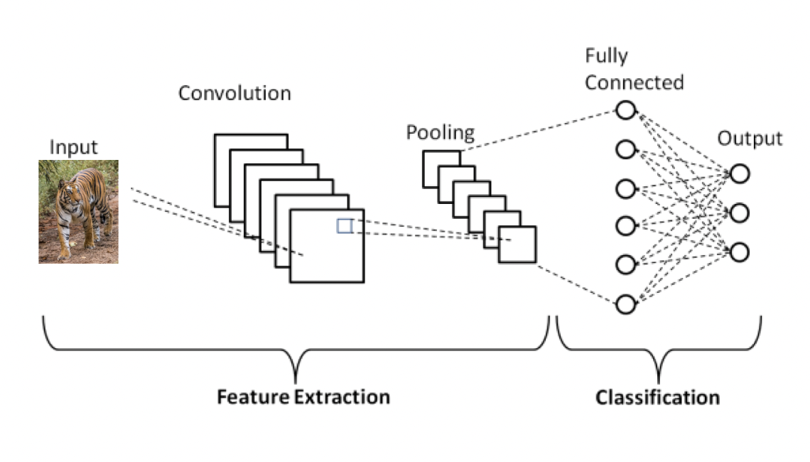
Figure 1: Convolutional Neural Network. [19]

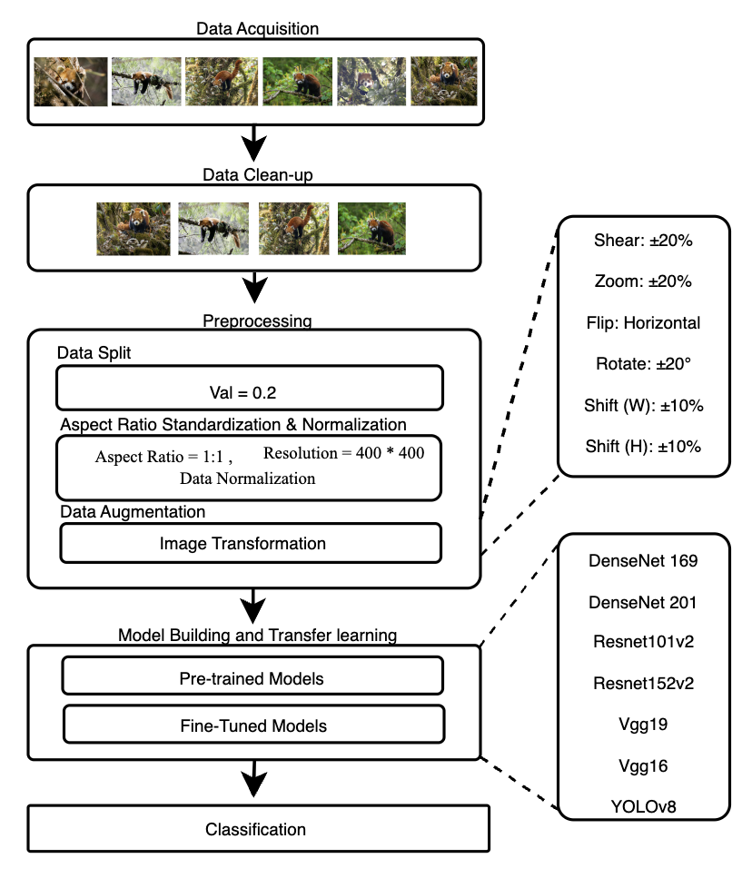
Figure 2: Methodology.

2.4 Transfer Learning

Transfer learning is an approach to deep learning that enables researchers and developers to use the previously trained model in a huge dataset and implement it in downstream tasks [22]. It is especially useful when we have limited data to train the model. Also, it significantly reduces the training time because the feature extraction part remains unchanged. However, it may fail when there is a significant mismatch between the target domain task and the source task.

These are some of the models we used to compare transfer learning with our dataset. Figure 3 shows the corresponding architecture of these models.

• DenseNet: DenseNet was introduced by Gao Huang and colleagues in 2017 [26]. It connects each layer with all other layers densely, meaning each layer receives input from the preceding layers. By efficiently cutting the parameters’ requirements and boosting the network’s ability by reusing the features extracted, it allows for a deeper network. However, the dense connectivity may lead to increased computational cost and memory consumption.

• ResNet: ResNet was introduced by Kaiming He et al. in 2016 [12]. It utilizes residual blocks, which are shortcut connections that bypass one or multiple layers. It also allows the network to learn residual functions instead of direct mapping. This architecture supports very deep networks without degradation problems.

• VGG: VGG was introduced by Karen Simonyan and Andrew Zisserman in 2014 [18]. It is known for its simplicity and depth, achieved by stacking small 3*3 convolutional layers, increasing the model’s depth and parameters. The max pooling layers follow the convolutional layers to handle the volume size and end with the fully connected layers.

  

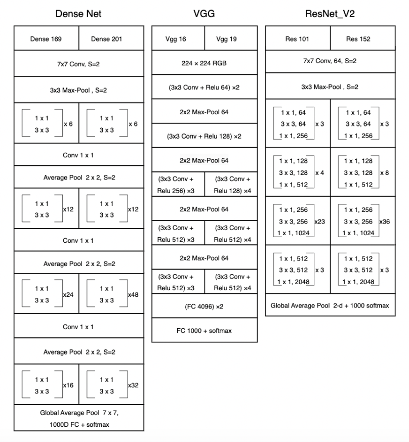
  Figure 3: Architecture of different models used in our study.

• YOLOv8: YOLOv8 is built upon the object detection framework introduced by Joseph Redmon, with contributions from many researchers over successive versions. It enhances speed and accuracy through an advanced backbone architecture, refined loss functions, and anchor-free detections [21]. Figure 4 shows the architecture of the YOLOv8.

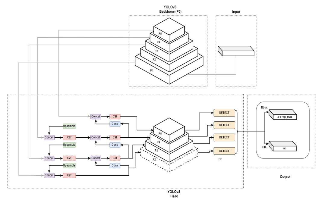
Figure 4: Reference image for YOLOv8 architecture.

2.5 Model Building

We loaded the pre-trained models(DenseNet, ResNet and VGG, ) with their respective weights, made these weights untrainable(frozen), and replaced the last layer with custom, fully connected layers corresponding to the number of classes in our dataset. We added a GlobalAveragePooling2D layer to reduce the feature maps’ spatial dimensions and prevent overfitting. This layer is followed by a Dense layer with 128 neurons and activated by ReLU to introduce non-linearity and learn more complex features. Finally, we added a Dense layer with 23 units activated by softmax to match the number of classes in our dataset, enabling the model to output the class probabilities, as shown in Figure 5. We then trained the models using Adam as the optimizer and cross-entropy as the loss function for 100 epochs with a batch size of 32 images. Meanwhile, we used a validation set to monitor the progress to avoid plateauing and adjusting the learning rate dynamically.

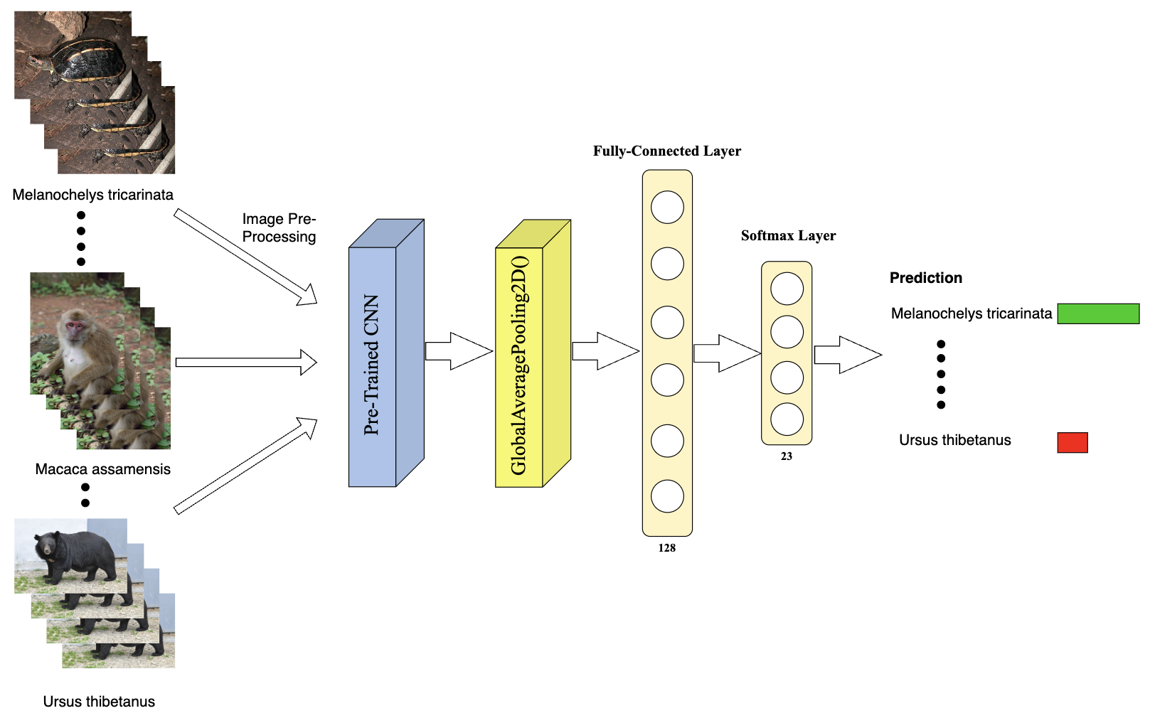
Figure 5: Illustration of transfer learning.

2.6 Hyperparameters

We experimented with multiple sets of hyperparameters, including learning rates, optimizers, batch sizes, and schedulers, thereby selecting the most favorable settings of hyperparameters that showed optimal performance. Table 3 lists the final set of hyperparameters.

• Categorical Cross Entropy: Categorical Cross Entropy (CCE) is used for multi-class classification tasks. It measures the difference between the true class labels and the predicted class probabilities. The formula sums the negative log-likelihood of the true class’s predicted probability across all classes. We have used CCE as our loss function.

  $$\text{Categorical Cross Entropy}=-\sum_{\text{neuron}=1}^{\text{classes}}y_{\text{true, neuron}}\cdot\ln(y_{\text{pred, neuron}})$$ (1)

• Binary Cross Entropy for One Neuron: Binary Cross Entropy (BCE) is used for binary classification tasks. The binary cross-entropy loss measures the dissimilarity between predicted probability distributions and the ground truth labels. The formula is the negative log-likelihood of the predicted probability if the true label is 1 and 1 minus the predicted probability if the true label is 0. The BCE is utilized in each output layer neuron and used in the YOLOv8 classification task.

  $$\text{BCE}_{\text{1neuron}}=-\left[y_{\text{true}}\cdot\ln(y_{\text{predicted}})+(1-y_{\text{true}})\cdot\ln(1-y_{\text{predicted}})\right]$$ (2)

• AdamW Optimizer: AdamW stands for Adaptive Moment Estimation with Weight Decay. It is an extension of the Adam optimizer, including weight decay, to improve generalization by preventing overfitting. AdamW adjusts the learning rate based on the gradients’ first and second moments and consists of a weight decay term to penalize large weights.

  $$\text{AdamW}:\Theta_{t+1}=\Theta_{t}-\alpha\cdot\frac{\mathbf{V}_{t}}{\sqrt{\mathbf{S}_{t}}+\epsilon}+\epsilon\cdot m_{t}-\alpha\cdot\text{weight\_decay}\cdot\Theta_{t}$$ (3)

  Where:

  • $\Theta_{t}$ is the parameter at time step $t$

  • $\alpha$ is the learning rate

  • $m_{t}$ is the biased first-moment estimate

  • $\mathbf{V}_{t}$ is the biased second raw moment estimate

  • $\epsilon$ is a small constant to prevent division by zero

  • weight_decay is the weight decay term [24].

Hyperparameters	Value
Learning Rate	Adaptive
Batch Size	32
Epochs	100
Early Stopping	{ReduceLROnPlateau, Validation Accuracy}
Optimizers	{Adam, AdamW}

Table 3: Hyperparameters.

3 Performance and Evaluation Metrics

The performance of our models is not examined by accuracy alone. In addition to accuracy, other metrics like f1-score, precision, recall, and loss were employed for the evaluation. Precision is an indicator of the accuracy of model predictions i.e., the ratio of the true positive predictions to the total number of positive predictions made by the model. The recall is an indicator of the model’s ability to identify all the relevant classes i.e., ratio of true positive predictions to the total number of actual positive instances. The F1 score provides the single value for the evaluation of the model and is the harmonic mean of precision and recall. The loss gives insights into how well the model’s prediction matches the true outcomes and is the difference between the predicted values and the actual values.

• $$\text{Accuracy}=\frac{\text{True Positives}+\text{True Negatives}}{\text{Total number of samples}}$$ (4)

• $$\text{Precision}=\frac{\text{True Positives}}{\text{True Positives}+\text{False Positives}}$$ (5)

• $$\text{Recall}=\frac{\text{True Positives}}{\text{True Positives}+\text{False Negatives}}$$ (6)

• $$\text{F1 Score}=2\cdot\frac{\text{Precision}\cdot\text{Recall}}{\text{Precision}+\text{Recall}}$$ (7)

4 Results And Discussion

4.1 Results

Our study evaluated multiple deep-learning models for identifying endangered animal species from wildlife images. The results show the varying performance across the models. YOLOv8 outperformed the other models, and the DenseNet and Resnet models also did well, as their results were close to those of YOLOv8. In contrast, the VGG and Vanilla CNN models faced significant challenges. Table 4 shows the performances of different models.

S.N	Model Name	Accuracy (%)	Loss	F1-Score (%)	Precision (%)	Recall (%)
1	DenseNet169	Train = 98.27, Val = 93.91	Train = 0.0265, Val = 0.0482	Train = 95.22, Val = 93.95	Train = 99.46, Val = 98.94	Train = 83.76, Val = 80.87
2	DenseNet201	Train = 98.80, Val = 92.17	Train = 0.0161, Val = 0.0386	Train = 96.36, Val = 92.22	Train = 99.95, Val = 94.62	Train = 89.97, Val = 76.52
3	Resnet101V2	Train = 98.74, Val = 92.17	Train = 0.0083, Val = 0.9217	Train = 97.36, Val = 92.09	Train = 99.42, Val = 98.00	Train = 95.72, Val = 85.22
4	Resnet152V2	Train = 98.20, Val = 93.04	Train = 0.0104, Val = 0.0271	Train = 95.79, Val = 93.22	Train = 99.19, Val = 97.14	Train = 94.01, Val = 88.70
5	VGG16	Train = 46.00, Val = 33.91	Train = 0.5619, Val = 0.5994	Train = 42.89, Val = 28.65	Train = 0.00, Val = 0.00	Train = 0.00, Val = 0.00
6	VGG19	Train = 32.67, Val = 33.04	Train = 0.6222, Val = 0.6449	Train = 29.82, Val = 31.19	Train = 0.00, Val = 0.00	Train = 0.00, Val = 0.00
7	YOLOv8	Train = 97.39, Val = 99.13	Train = 0.0118, Val = NA	Train = 96.50, Val = 99.12	Train = 96.81, Val = 99.28	Train = 96.52, Val = 99.13

Table 4: Performance of different deep learning models on our dataset.

• DenseNet: DenseNet architectures showed strong performance across all metrics. DenseNet 169 achieved a training accuracy of 98.27% and a validation accuracy of 93.91%. Also, it had F1 scores of 95.22% in training and 93.95% in validation. Impressively, DenseNet 201 outperformed by a slightly better training accuracy of 98.80% and had F1-scores of 96.36% in training and 92.22% in validation, though its validation accuracy was somewhat lower at 92.17%.

  Figure 7 shows training and validation set loss curves decreasing rapidly, finally reaching a plateau, indicating good learning and model convergence. The relatively smooth curve showed a minimal gap in Figure 7, indicating good generalization and no significant overfitting.

  

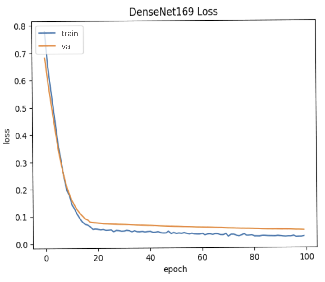
  Figure 6: Loss curve of DenseNet169.

  

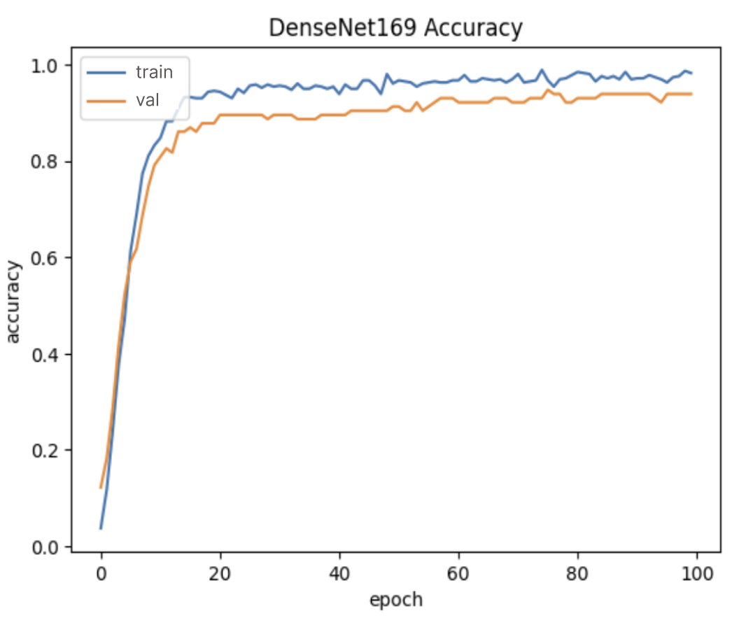
  Figure 7: Accuracy curve of DenseNet169.

• ResNet: The ResNets architecture also showed promising results. Resnet 101 V2 reached a training accuracy of 98.74% and a validation accuracy of 92.17%. Its F1 scores were 97.36% in training and 92.09% in validation, showing robust performance. Resnet 152 V2 showed a training accuracy of 98.20% and a validation accuracy of 93.04%, with high F1-scores of 95.79% in training and 93.22% in validation.

  The training and validation data loss plunged drastically initially and finally tended towards low values, similar to DenseNet169, as shown in Figure 9. The very close train and validation loss curves indicated that the model generalized well without overfitting—a similar trend in the training and validation accuracy from Figure 9.

  

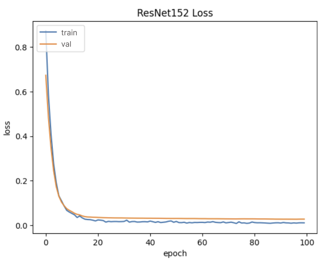
  Figure 8: Loss curve of ResNet152.

  

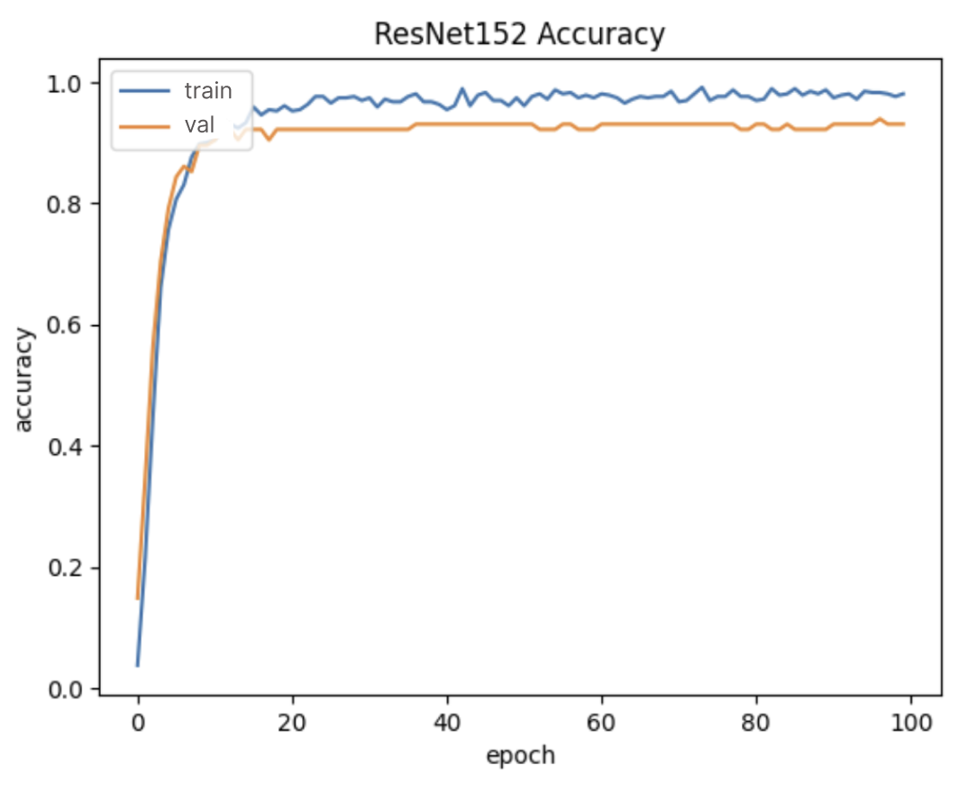
  Figure 9: Accuracy curve of ResNet152.

• VGG: In contrast, the VGG architectures underperformed significantly compared to DenseNet and ResNet models. VGG 16 and VGG 19 showed much lower training accuracies (46.00% and 32.67%, respectively) and validation accuracies (33.91% and 33.04%, respectively). Their F1 scores were also considerably lower, with VGG 16 at 42.89% for training and 28.65% for validation and VGG 19 at 29.82% for training and 31.19% for validation.

  The training loss decreased steadily, while the validation loss followed a different pattern, decreasing even slower and with apparent variance, as shown in Figure 11. There was a visible gap between training and validation loss, showing the possible overfitting phenomenon, i.e., a model fitting much better with the training set than the validation set. Also, Figure 11 shows oscillations in the training and validation accuracies.

  

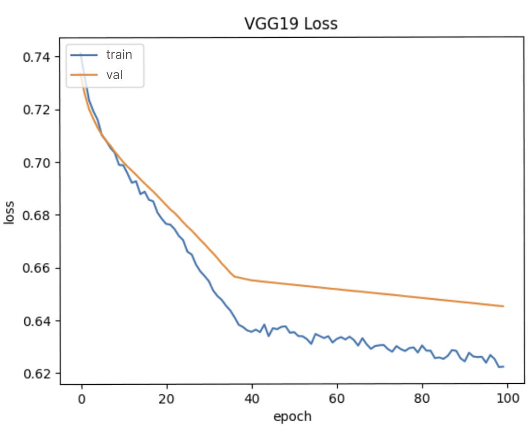
  Figure 10: Loss curve of VGG19.

  

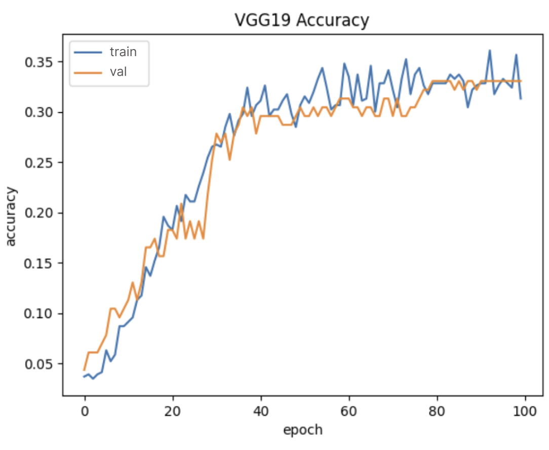
  Figure 11: Accuracy curve of VGG19.

• YOLOv8: The YOLOV8 model achieved an accuracy of 97.39% in training and 99.13% in validation with a shallow loss of 0.01175, which showed that despite being known for detection purposes, it surprisingly worked well for our classification task. The F1 score was 96.5% in training and 99.12% in validation.

  Figure 13 shows that the loss decreased rapidly and plateaued early in training, which shows the model’s effectiveness for fast convergence during transfer learning. Unlike the loss, the accuracy oscillated slightly before it finally plateaued near 50 epochs, as indicated in Figure 13.

  

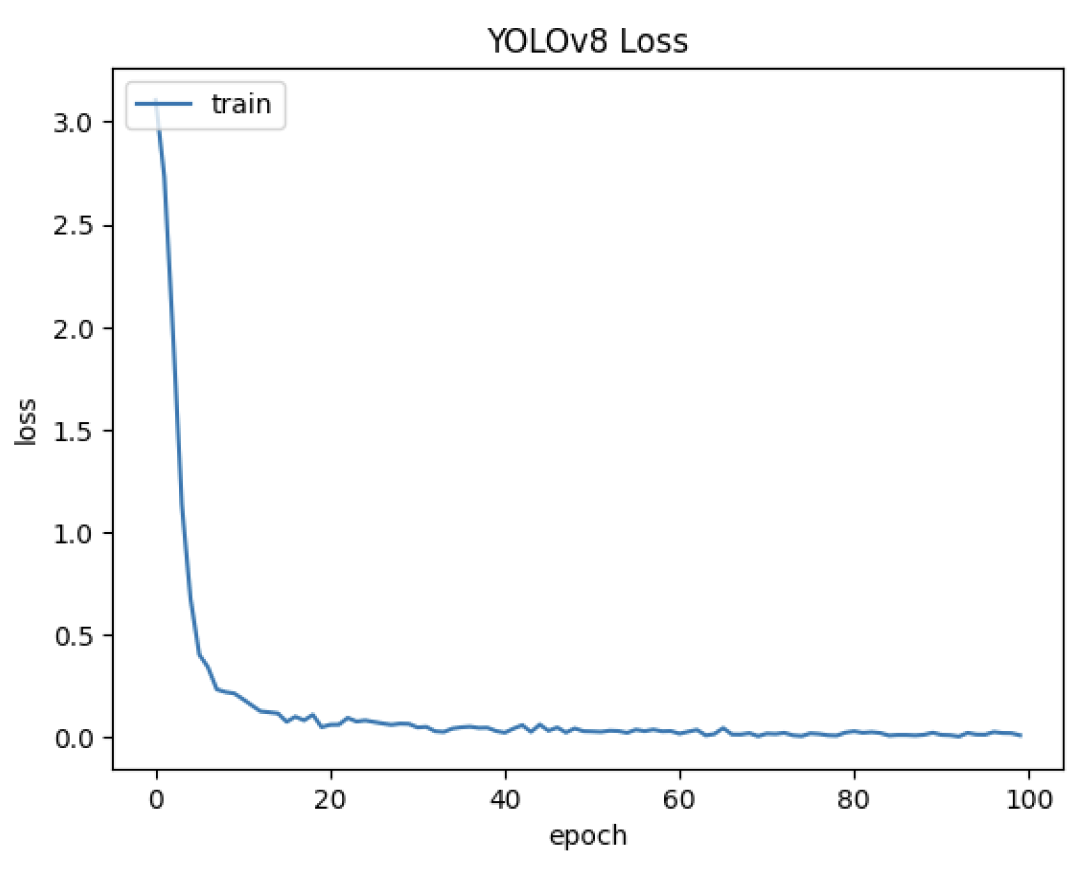
  Figure 12: Loss curve of YOLOv8.

  

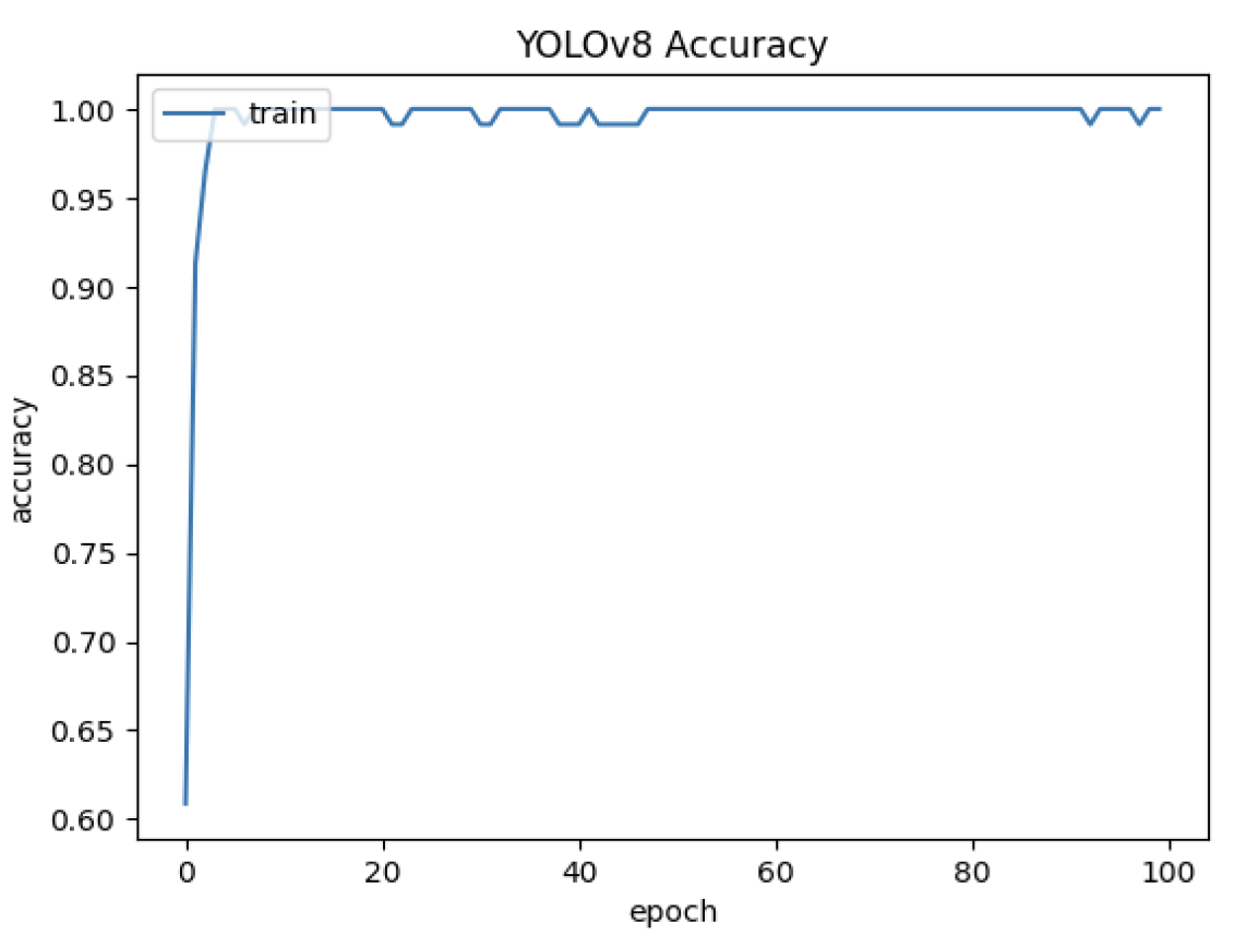
  Figure 13: Accuracy curve of YOLOv8.

• CNN: We validated different architectures for the vanilla CNN with the same dataset. However, we did not get satisfactory results. Since our dataset contained images of species across 23 classes, simple, shallow CNN could not converge effectively. Nevertheless, we tried adjusting various parameters like the number of layers, regularization techniques, loss functions, and augmentations. Despite these efforts, the performance metrics remained mediocre.

4.2 Discussions

Our experimental analysis shows the metrics of various deep-learning models in identifying endangered animals on our custom endangered wildlife dataset, as shown in Figure 14. The dataset was carefully created from reputable online databases, ensuring the species’ authenticity and relevance. Our motto was to train a model that could recognize vulnerable species and assist in their proper monitoring. Furthermore, the other side of our study involved finding the best available architecture for this task. We experimented with various such architectures and analyzed their performance under different metrics.

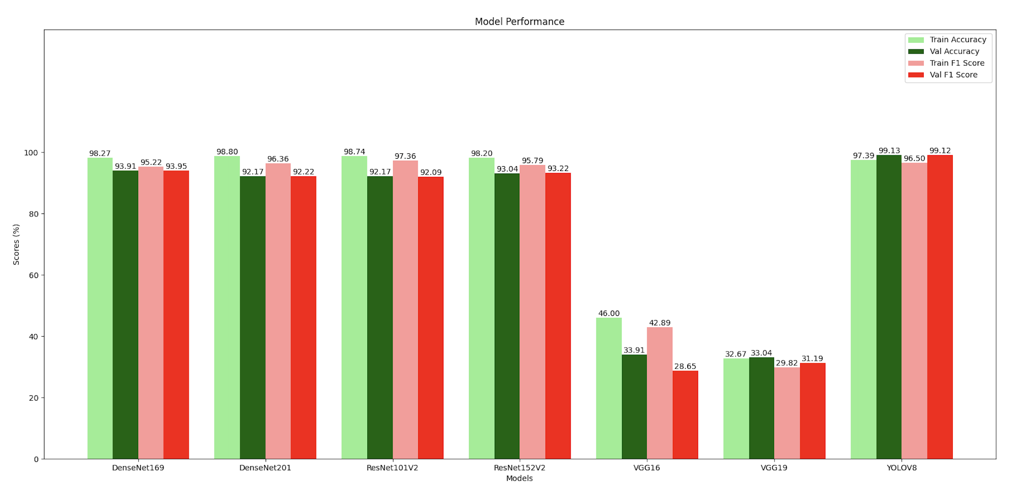
Figure 14: Comparison of metrics for different models.

We found that newer version of all the models showed stronger performance. VGG was the oldest among our models, so it performed poorly. Its accuracy was way below the vanilla CNN. Conversely, DenseNet and ResNet offered significantly better performance, so we can easily use them for related tasks. Also, we noted that these networks’ newer and deeper versions did not provide any impactful difference across various metrics.
In addition, we implemented transfer learning and did not train them from scratch, benchmarking their ease of use in downstream tasks like ours. We had to freeze the feature extraction layers and only trained the last few fully connected layers. Doing this saved the time and computing required without compromising their performance.
Alongside standard CNN models like ResNet, DenseNet, and VGGNet, specially designed for classification tasks, we also experimented with YOLOv8. YOLOs are primarily designed and used as go-to models for detection and segmentation tasks. To our great surprise, the metrics surpassed other standard classification models. Thus, YOLO might work well for classification tasks for custom datasets in similar niches. Why does YOLOv8 perform the best? YOLOv8’s superior performance might be due to its advanced architecture, which combines efficient feature extraction with fast processing capabilities by integrating components like CSPNet (Cross Stage Partial Networks) and PANet (Path Aggregation Network) [28, 15]. CSPNet reduces the computational cost while maintaining accuracy. It divides the feature map into two parts and merges them through the cross-stage hierarchy. On the other hand, PANet enhances the information flow between various layers, which is excellent for object detection across multi-scales. But, this proved beneficial for classification tasks, too. Even more importantly, the multiscale capability of YOLOv8 allows handling images with object sizes that can have significant variations and differing resolutions. It also has advanced augmentations, such as mosaic augmentation, which places four training images into one with diverse contexts in one image and hence helps the model generalize better to varying lighting and environmental conditions in training. All these features, together, carry out fast processing and effective feature extraction.

5 Conclusion

To sum up, we performed experimental analysis on transfer learning of various deep-learning CNN architectures on our custom dataset containing images of endangered mammals from Nepal. Our findings featured the superior performance of YOLOv8 compared to other models like DenseNet, ResNetV2, and VGG. It demonstrated higher accuracy, precision, and recall, making it practical for our and similar classification tasks. Although lagging by a narrow margin, other models like ResNet and DenseNet also performed well and competed neck and neck with YOLOv8. Transfer learning proved beneficial, drastically reducing training time and data required while maintaining high performance, which is crucial for tasks with limited data availability.
In the future, we will explore the ensemble methods that combine the strengths of multiple CNN architectures potentially enhancing classification accuracy and robustness, especially in diverse and challenging environmental conditions. We will also incorporate real-time monitoring capabilities in the future to provide feedback for conservation and take timely action in preventing the loss of endangered species. Hence, this study shows the reliance and robustness of deep-learning models in monitoring wildlife.

6 Funding

This research received no external funding.

7 Conflicts of Interest

The authors declare that there is no conflict of interest regarding the publication of this paper.

8 Acknowledgment

The authors thank their supervisor, Dr. Mansi Bhavsar, for their invaluable guidance and support. Both authors contributed equally to this work.

References

- Babu et al., [2024] Babu, M. A. A., Pandey, S. K., Durisic, D., Koppisetty, A. C., and Staron, M. (2024). Impact of image data splitting on the performance of automotive perception systems. In International Conference on Software Quality, pages 91–111. Springer.
- Beery et al., [2018] Beery, S., Van Horn, G., and Perona, P. (2018). Recognition in terra incognita. In Proceedings of the European conference on computer vision (ECCV), pages 456–473.
- Brust et al., [2017] Brust, C.-A., Burghardt, T., Groenenberg, M., Kading, C., Kuhl, H. S., Manguette, M. L., and Denzler, J. (2017). Towards automated visual monitoring of individual gorillas in the wild. In Proceedings of the IEEE International Conference on Computer Vision Workshops, pages 2820–2830.
- Caldas, [2021] Caldas, C. (2021). split-folders (version 0.5.1). Available at: https://pypi.org/project/split-folders/.
- Chauhan et al., [2018] Chauhan, R., Ghanshala, K. K., and Joshi, R. (2018). Convolutional neural network (cnn) for image detection and recognition. In 2018 first international conference on secure cyber computing and communication (ICSCCC), pages 278–282. IEEE.
- El Abbadi and Alsaadi, [2020] El Abbadi, N. K. and Alsaadi, E. M. T. A. (2020). An automated vertebrate animals classification using deep convolution neural networks. In 2020 International Conference on Computer Science and Software Engineering (CSASE), pages 72–77. IEEE.
- He et al., [2016] He, K., Zhang, X., Ren, S., and Sun, J. (2016). Deep residual learning for image recognition. In Proceedings of the IEEE conference on computer vision and pattern recognition, pages 770–778.
- Huang et al., [2017] Huang, G., Liu, Z., Van Der Maaten, L., and Weinberger, K. Q. (2017). Densely connected convolutional networks. In Proceedings of the IEEE conference on computer vision and pattern recognition, pages 4700–4708.
- Ibraheam et al., [2020] Ibraheam, M., Gebali, F., Li, K. F., and Sielecki, L. (2020). Animal species recognition using deep learning. In Advanced Information Networking and Applications: Proceedings of the 34th International Conference on Advanced Information Networking and Applications (AINA-2020), pages 523–532. Springer.
- iNaturalist, [2022] iNaturalist (2022). iNaturalist. https://inaturalist.org/.
- Jnawali et al., [2011] Jnawali, S., Baral, H., Lee, S., Acharya, K., Upadhyay, G., Pandey, M., and Griffiths, J. (2011). The status of nepal mammals: the national red list series, department of national parks and wildlife conservation kathmandu, nepal. Preface by Simon M. Stuart Chair IUCN Species Survival Commission The Status of Nepal’s Mammals: The National Red List Series, 4.
- Krizhevsky et al., [2012] Krizhevsky, A., Sutskever, I., and Hinton, G. E. (2012). Imagenet classification with deep convolutional neural networks. Advances in neural information processing systems, 25.
- Kumar et al., [2022] Kumar, M., Yadav, A. K., Kumar, M., and Yadav, D. (2022). Bird species classification from images using deep learning. In International Conference on Computer Vision and Image Processing, pages 388–401. Springer.
- LeCun et al., [1998] LeCun, Y., Bottou, L., Bengio, Y., and Haffner, P. (1998). Gradient-based learning applied to document recognition. Proceedings of the IEEE, 86(11):2278–2324.
- Liu et al., [2018] Liu, S., Qi, L., Qin, H., Shi, J., and Jia, J. (2018). Path aggregation network for instance segmentation. In Proceedings of the IEEE conference on computer vision and pattern recognition, pages 8759–8768.
- Lu et al., [2021] Lu, J., Tan, L., and Jiang, H. (2021). Review on convolutional neural network (cnn) applied to plant leaf disease classification. Agriculture, 11(8):707.
- Nguyen et al., [2017] Nguyen, H., Maclagan, S. J., Nguyen, T. D., Nguyen, T., Flemons, P., Andrews, K., Ritchie, E. G., and Phung, D. (2017). Animal recognition and identification with deep convolutional neural networks for automated wildlife monitoring. In 2017 IEEE international conference on data science and advanced Analytics (DSAA), pages 40–49. IEEE.
- Pan and Yang, [2009] Pan, S. J. and Yang, Q. (2009). A survey on transfer learning. IEEE Transactions on knowledge and data engineering, 22(10):1345–1359.
- Phung and Rhee, [2018] Phung, V. H. and Rhee, E. J. (2018). A deep learning approach for classification of cloud image patches on small datasets. Journal of information and communication convergence engineering, 16(3):173–178.
- Redmon et al., [2016] Redmon, J., Divvala, S., Girshick, R., and Farhadi, A. (2016). You only look once: Unified, real-time object detection. In Proceedings of the IEEE conference on computer vision and pattern recognition, pages 779–788.
- Reis et al., [2023] Reis, D., Kupec, J., Hong, J., and Daoudi, A. (2023). Real-time flying object detection with yolov8. arXiv preprint arXiv:2305.09972.
- Russakovsky et al., [2015] Russakovsky, O., Deng, J., Su, H., Krause, J., Satheesh, S., Ma, S., Huang, Z., Karpathy, A., Khosla, A., Bernstein, M., et al. (2015). Imagenet large scale visual recognition challenge. International journal of computer vision, 115:211–252.
- Sharma et al., [2024] Sharma, S., Ghimire, R., Gurung, S., and GC, S. (2024). Gantavya: A landmark recognition system.
- Shorten and Khoshgoftaar, [2019] Shorten, C. and Khoshgoftaar, T. M. (2019). A survey on image data augmentation for deep learning. Journal of big data, 6(1):1–48.
- Simonyan and Zisserman, [2014] Simonyan, K. and Zisserman, A. (2014). Very deep convolutional networks for large-scale image recognition. arXiv preprint arXiv:1409.1556.
- Szegedy et al., [2015] Szegedy, C., Liu, W., Jia, Y., Sermanet, P., Reed, S., Anguelov, D., Erhan, D., Vanhoucke, V., and Rabinovich, A. (2015). Going deeper with convolutions. In Proceedings of the IEEE conference on computer vision and pattern recognition, pages 1–9.
- Villa et al., [2017] Villa, A. G., Salazar, A., and Vargas, F. (2017). Towards automatic wild animal monitoring: Identification of animal species in camera-trap images using very deep convolutional neural networks. Ecological informatics, 41:24–32.
- Wang et al., [2020] Wang, C.-Y., Liao, H.-Y. M., Wu, Y.-H., Chen, P.-Y., Hsieh, J.-W., and Yeh, I.-H. (2020). Cspnet: A new backbone that can enhance learning capability of cnn. In Proceedings of the IEEE/CVF conference on computer vision and pattern recognition workshops, pages 390–391.
- Yılmaz et al., [2021] Yılmaz, A., Uzun, G. N., Gürbüz, M. Z., and Kıvrak, O. (2021). Detection and breed classification of cattle using yolo v4 algorithm. In 2021 International Conference on INnovations in Intelligent SysTems and Applications (INISTA), pages 1–4. IEEE.
- ZooChat, [2002] ZooChat (2002). ZooChat: The world’s largest community of zoo and animal conservation enthusiasts. https://www.zoochat.com/community/.