A sharp lower bound on the small eigenvalues of surfaces

Abstract

Let ${S}$ be a compact hyperbolic surface of genus $g\geq 2$ and let $I({S})=\frac{1}{\mathrm{Vol}({S})}\int_{{S}}\frac{1}{\mathrm{Inj}\left(x\right)^{2}\wedge 1}dx$, where $\mathrm{Inj}\left(x\right)$ is the injectivity radius at $x$. We prove that for any $k\in\{1,\ldots,2g-3\}$, the $k$-th eigenvalue $\lambda_{k}$ of the Laplacian satisfies

$$\lambda_{k}\geq\frac{ck^{2}}{I({S})g^{2}}\,,$$

where $c>0$ is some universal constant. We use this bound to prove the heat kernel estimate

$$\frac{1}{\mathrm{Vol}({S})}\int_{S}\Big{|}p_{t}(x,x)-\frac{1}{\mathrm{Vol}({S})}\Big{|}\leavevmode\nobreak\ dx\leq C\sqrt{\frac{I({S})}{t}}\qquad\forall t\geq 1\,,$$

where $C<\infty$ is some universal constant. These bounds are optimal in the sense that for every $g\geq 2$ there exists a compact hyperbolic surface of genus $g$ satisfying the reverse inequalities with different constants.

1 Introduction

Let ${S}$ be a compact hyperbolic surface of genus $g\geq 2$. Due to compactness, the Laplacian has a discrete spectrum $0=\lambda_{0}<\lambda_{1}\leq\lambda_{2}\leq\ldots$ with $\lambda_{j}\to\infty$ as $j\to\infty$. The eigenvalues below $1/4$ are usually called small, see [Hub61, p386] and [Bus10, Chapter 8]. A classical construction of Buser [Bus77] shows that for any $\varepsilon>0$ and any $g\geq 2$ there exists such a compact hyperbolic surface ${S}$ of genus $g$ with $\lambda_{k}\leq\varepsilon$ for all $k=1,\ldots,2g-3$. Otal and Rosas [OR09] showed that $\lambda_{2g-2}>1/4$ for any ${S}$, hence only the first $2g-3$ eigenvalues can be small. Here we provide a sharp estimate as to how small the small eigenvalues can be in terms of $k$ and $g$ and the quantity $I({S})=\frac{1}{\mathrm{Vol}({S})}\int_{{S}}\frac{1}{\mathrm{Inj}\left(x\right)^{2}\wedge 1}dx$, where $\mathrm{Inj}\left(x\right)$ is the injectivity radius at $x$.

Theorem 1.

There exists a universal constant $c>0$ such that for any compact hyperbolic surface ${S}$ of genus $g\geq 2$ and every $k\in\{1,\ldots,2g-3\}$,

$$\lambda_{k}\geq\frac{ck^{2}}{I({S})g^{2}}\,.$$ (1)

We use this estimate to provide a uniform bound on the heat kernel trace on ${S}$.

Theorem 2.

For any compact hyperbolic surface ${S}$

$$\frac{1}{\mathrm{Vol}({S})}\int_{S}\Big{|}p_{t}(x,x)-\frac{1}{\mathrm{Vol}({S})}\Big{|}\leavevmode\nobreak\ dx\leq C\sqrt{\frac{I({S})}{t}}\qquad\forall t\geq 1\,.$$ (2)

where $p_{t}^{{S}}(x,y)$ is the heat kernel of the Laplacian on ${S}$ and $C<\infty$ is a universal constant.

We also show that Theorem 1 and Theorem 2 are optimal in the sense that for any $g\geq 2$ and $I\geq 1$, there exists a compact hyperbolic surface ${S}$ of genus $g$ and $I(S)\geq I$ such that the reversed inequalities of (1) and (2) holds with a different constant.

We remark that $I({S})$ has an additional simple geometric interpretation. Let $\gamma_{1},\ldots,\gamma_{s}$ be the set of all simple closed geodesics in ${S}$ of length at most $2\sinh^{-1}(1)$ and denote by $\{\ell(\gamma_{i})\}_{i=1}^{s}$ their lengths. Then it is not hard to prove (see Corollary 9) that

$$I({S})\asymp 1+\frac{1}{\mathrm{Vol}({S})}\sum_{i=1}^{s}\frac{1}{\ell(\gamma_{i})}\,.$$

1.1 Related work

A classical paper of Schoen, Wolpert and Yau [SWY80] provides the bound $\lambda_{k}\geq\alpha(g)L_{k}({S})$, where $\alpha(g)$ is an unknown function of $g$, and $L_{k}({S})$ is the minimal possible sum of the lengths of simple closed geodesics in ${S}$ that cut ${S}$ into $k+1$ components. In order to improve the dependence on $g$ of this bound, it is shown in [WX22] that $\lambda_{1}\gtrsim L_{1}({S})/g^{2}$ and in [HW24] that $\lambda_{2}\gtrsim L_{2}({S})/g^{2}$.

We remark that while both quantities $L_{k}({S})$ and $1/I({S})$ measure the amount of bottlenecks in a surface (see Corollary 9), they are in general incomparable. Whenever the injectivity radius is uniformly bounded below, Theorem 1 implies that $\lambda_{k}\gtrsim k^{2}/g^{2}$ for $k\in\{1,\ldots,2g-3\}$ improving a result obtained in [WX22a] regarding such lower bounds in any thick part of the moduli space.

On-diagonal heat kernel bounds such as (2) are a well studied topic going back to Nash, Moser and Varopoulos, see [Gri94, Gri09, Gri99]. They are classically proved using a suitable isoperimetric inequality and typically yield a uniform estimate in $x$. In this paper, however, one can see that isoperimetric inequalities are irrelevant; for example, one can take $O(1)$ primitive closed geodesic of length $\Theta(1)$, pinch them so that their length is $\Theta(1/g)$ and $I({S})$ will remain of the same order, leaving the bounds of Theorems 1 and 2 unaltered. Additionally, one cannot hope for a bound on the on-diagonal heat kernel that is uniform in $x$ without some global isoperimetric inequality.

1.1.1 Discrete analogue

Laplacian eigenvalues and heat kernel bounds are a well studied topic in the discrete setting as well. Let $G$ be a simple, connected, regular graph with $n$ vertices and consider the lazy random walk on it, that is, the walker moves to a uniformly drawn neighbor with probability $1/2$ or stays put otherwise. Let $P$ denote its transition probability matrix. The graph Laplacian $\mathcal{L}=I-P$ has eigenvalues $0=\lambda_{0}<\lambda_{1}\leq\ldots\lambda_{n-1}\leq 1$. The bound

$$\lambda_{k}\gtrsim\frac{k^{2}}{n^{2}}\,,$$ (3)

for all $k\in\{1,\ldots,n\}$ is well known, and follows directly from the estimate (see [CKS87, Cou00, Lyo05, LO18]):

$$\frac{1}{n}\Big{|}\sum_{x}P^{t}(x,x)-1\Big{|}\lesssim\frac{1}{\sqrt{t}}\,,$$ (4)

for any integer $t\geq 1$ (this is the discrete analogue of (2)). Indeed, recalling that $\sum_{x}P^{t}(x,x)=\sum_{i=0}^{n-1}(1-\lambda_{i})^{t}$ and plugging in $t=\lceil\lambda_{k}^{-1}\rceil$ to the above immediately yields (3). In this setup it is also known that the $t^{-1/2}$ upper bound on $|P^{t}(x,x)-n^{-1}|$ holds uniformly in $x$. Of course we cannot hope for the bound (3) to be valid for all surfaces, nor can we expect a uniform bound in $x$ for same reason, namely, the possibility of arbitrarily small bottlenecks.

Thus, the more appropriate discrete analogue are finite weighted graphs. In this setting, bounds on the spectral measure at a vertex were given by Lyons and Oveis Gharan [[]Corollary 4.8]lyons_oveis_gharan_sharp_bounds_via_spectral_embedding. Similar bounds were obtained by Lyons and Judge [JL19] in the setup of homogenous Riemannian manifolds. We were greatly inspired by the use of the spectral kernel in [LO18]; as done there, we too bound the eigenvalues by the Dirichlet energy of a function associated with the spectral kernel, but the bulk of this paper is dedicated to bounding below this energy using a novel geometric argument based on extremal length.

1.2 Extremal length

Extremal length is a geometric method in complex analysis that has had a profound influence on the theory of conformal and quasi-conformal mappings. In this paper we obtain an explicit geometric bound on the extremal length between two small geodesic discs placed at arbitrary locations in ${S}$. Given a Borel measurable function $\rho:{S}\to[0,\infty)$ and a rectifiable curve $\gamma\subseteq{S}$, the $\rho$-length of $\gamma$ is

$$L(\gamma,\rho)=\int_{\gamma}\rho\leavevmode\nobreak\ |dz|\,.$$

Definition 3 (Extremal length).

Given a collection $\Gamma$ of rectifiable curves in ${S}$ we define the extremal length of $\Gamma$ as

$$\mathsf{EL}\left(\Gamma\right)=\sup_{\rho}\frac{\inf_{\gamma\in\Gamma}L(\gamma,\rho)^{2}}{\int_{{S}}\rho^{2}\leavevmode\nobreak\ d\mu}\,,$$

where the supremum is taken over all Borel measurable functions $\rho:{S}\to[0,\infty)$ and $\mu$ is the Riemannian area measure of ${S}$.

For a general compact Riemannian manifold $M$, the injectivity radius of a point $x\in M$, denoted $\mathrm{Inj}\left(x,M\right)$, is the supremum radius such that the exponential map $\exp_{x}$ is a diffeomorphism. We often write $\mathrm{Inj}\left(x\right)$ when it is clear what $M$ is from the context. The injectivity radius of the manifold $M$ itself is $\mathrm{Inj}\left(M\right)=\inf_{x\in M}\mathrm{Inj}\left(x,M\right)$. When ${S}$ is a Riemannian surface of constant curvature $-1$, i.e., a hyperbolic surface, $\mathrm{Inj}\left(x,{S}\right)$ is the supremum $r$ so that the ball of radius $r$ around $x$ is isometric to the ball of radius $r$ in the hyperbolic plane ${\mathbb{H}}$.

Definition 4 (Reciprocal-injectivity weight).

For $x\in{S}$, let

$$\widehat{\mathrm{Inj}}\left({x}\right)=\mathrm{Inj}\left(x,{S}\right)\land 1\,.$$

For a rectifiable curve $\gamma\subseteq{S}$, let

$$w\left(\gamma\right)=\int_{\gamma}\widehat{\mathrm{Inj}}\left({z}\right)^{-1}|dz|\,.$$

This lets us define the weighted distance between $x$ and $y$ as

$$\mathrm{dist}_{w}\left(x,y\right)=\inf_{\gamma}w\left(\gamma\right)\,,$$

where the infimum ranges over all rectifiable curves $\gamma$ which connect $x$ to $y$.

Our main geometric result is the following.

Theorem 5.

Let $x,y\in{S}$ and $r_{x},r_{y}$ be positive numbers satisfying

$$d_{S}(x,y)\geq r_{x}+r_{y}\,,\quad r_{x}\leq\widehat{\mathrm{Inj}}\left({x}\right)/2\,,\quad r_{y}\leq\widehat{\mathrm{Inj}}\left({y}\right)/2\,.$$

Let $\Gamma$ be the set of all curves in ${S}\backslash\left(B(x,r_{x})\cup B(y,r_{y})\right)$ from $\partial B(x,r_{x})$ to $\partial B(y,r_{y})$. Then

$$\mathsf{EL}\left(\Gamma\right)\lesssim\mathrm{dist}_{w}\left(x,y\right)+\log\left(\frac{\widehat{\mathrm{Inj}}\left({x}\right)}{r_{x}}\right)+\log\left(\frac{\widehat{\mathrm{Inj}}\left({y}\right)}{r_{y}}\right)\,.$$ (5)

Remark 6.

Let us provide a rough, yet guiding, intuition. It is well known that any compact hyperbolic surface ${S}$ has a pair of pants decomposition in which all simple closed geodesics of length at most $2\sinh^{-1}(1)$ are boundary geodesics where two pairs of pants were glued. This is the content of the so-called collar lemma (Lemma 7). If a path $\gamma$ traverses from one side of a narrow collar of width $\ell$ to the other, then the contribution of this part of the curve to its weight $w\left(\gamma\right)$ is proportional to $1/\ell$. Thus, $w\left(\gamma\right)$ is the sum of the reciprocal lengths of the narrow collars through which it passes, up to a multiplicative constant.

We may think of this pair of pants decomposition of ${S}$ as defining a $3$-regular graph in which the pants are vertices and edges are formed between two pairs of pants if they are glued at one of their three boundary geodesics. Assign to each edge a weight $c_{e}$ equal to the length of the corresponding boundary geodesic. The weighted distance between two vertices $x,y$ in this analogous discrete setting is the minimal sum of reciprocals edge weights $1/c(e)$ over all paths from $x$ to $y$.

If the weights $\{c_{e}\}$ are thought of as electric conductances assigned to the edges, then by the parallel law together with Rayleigh’s monotonicity law, the effective electric resistance between $x$ and $y$ is at most the sum of edge resistances, i.e. $1/c(e)$, over the edges of any path from $x$ to $y$. So the weighted distance between two vertices $x$ and $y$ gives an upper bound on the effective electric resistance (this bound is far from sharp in many cases). Extremal length is the continuous analogue of effective electric resistance and so Theorem 5 is a very rough analogue of the aforementioned bound.

Notation and organization

For two non-negative functions $f(x)$ and $g(x)$, we write $f\lesssim g$ to mean that there exists a universal constant $C>0$, such that $f(x)\leq Cg(x)$ for all $x$. We write $f(x)\asymp g(x)$ if both $f\lesssim g$ and $g\lesssim f$. We denote the distance between two points in ${S}$ by $\mathrm{dist}_{{S}}\left(x,y\right)$. If $\gamma$ is a rectifiable curve in $S$, we denote its length by $\ell(\gamma)$.

The rest of this paper is organized as follows. In the next section, we provide the necessary geometric background. In Section 3 we prove Theorem 5 and in Section 4 we use it to prove Theorem 1. Theorem 2 is proved in Section 5 and optimality of Theorem 1 and Theorem 2 is shown in Section 6.

2 Geometric preliminaries

An important geometric characterization of hyperbolic surfaces is the so-called collar lemma, which describes the parts of the surface with small injectivity radius. The following is a combination of Theorem 4.1.1 and Theorem 4.1.6 from [Bus10].

Lemma 7 (Collar lemma).

Let $\gamma_{1},\ldots,\gamma_{s}$ be the set of all simple closed geodesics of length $\leq 2\sinh^{-1}(1)$ on a hyperbolic surface ${S}$. Let $W(\gamma_{i})=\sinh^{-1}\left(\frac{1}{\sinh\left(\frac{1}{2}\ell(\gamma_{i})\right)}\right)$ and $C(\gamma_{i})=\{x\in{S}\mid\mathrm{dist}(x,\gamma_{i})\leq W(\gamma_{i})\}$. Then

• The sets $C(\gamma_{i})_{i=1}^{s}$ are pairwise disjoint.

• $\mathrm{Inj}\left(x\right)\geq\sinh^{-1}(1)$ for all $x\notin\cup_{i}C(\gamma_{i})$.

• Each $C(\gamma_{i})$ is isometric to the cylinder $\left[-W(\gamma_{i}),W(\gamma_{i})\right]\times(\mathbb{R}/2\pi)$ with the Riemannian metric $ds^{2}=d\rho^{2}+\ell(\gamma_{i})^{2}\cosh(\rho)^{2}d\theta^{2}$.

• If $x\in C(\gamma_{i})$ and $d=\mathrm{dist}(x,\partial C(\gamma_{i}))$, then

  $$\sinh(\mathrm{Inj}\left(x\right))=\cosh\left(\frac{1}{2}\ell(\gamma_{i})\right)\cosh(d)-\sinh(d).$$

The following proposition provides a formula and an estimate of the injectivity radius of points in the collars in terms of their cylindrical coordinates.

Proposition 8 (Injectivity radius estimate).

Let $T$ be an infinite hyperbolic collar whose shortest closed geodesic $\gamma$ has length $\ell$. Denote by $r(\rho,\ell)$ the injectivity radius at a point of distance $\rho$ from $\gamma$. Then

$$r(\rho,\ell)=\frac{1}{2}\cosh^{-1}\left(1+\left(\cosh(\ell)-1\right)\cosh(\rho)^{2}\right)\,.$$

In particular,

$$r(\rho,\ell)\asymp\ell\cosh(\rho)\,$$

for all $\ell\leq 2\sinh^{-1}(1)$ and all $\rho\leq W(\gamma)$ where $W(\gamma)$ is defined in Lemma 7.

Proof.

In the upper-half plane model, an infinite collar can be realized as the quotient of ${\mathbb{H}}$ by the relation $x\sim\lambda x$, where $\lambda\in\mathbb{R}$ is chosen such that the hyperbolic distance satisfies $d_{{\mathbb{H}}}(i,\lambda i)=\ell$. Since $i$ and $\lambda i$ are on the imaginary axis, a simple integration gives $\log(\lambda)=\ell$. The injectivity radius is then given by $\frac{1}{2}d_{{\mathbb{H}}}(x,e^{\ell}x)$. To calculate this quantity, let $x$ be a point in the upper-half plane whose hyperbolic distance from the imaginary axis is $\rho$. Let $r=|x|$, so that $d_{{\mathbb{H}}}(x,ir)=\rho$. The distance between two points in the upper-half plane is given by

$$\cosh(d_{{\mathbb{H}}}(z,w))=1+\frac{|z-w|^{2}}{2\mathrm{Im}\left(z\right)\mathrm{Im}\left(w\right)}\,.$$

This lets us find the imaginary part of $x$. Using the distance formula, we have

$$\cosh(\rho)-1 =\cosh(d_{{\mathbb{H}}}(x,ir))-1$$

$$=\frac{|x-ir|^{2}}{2\mathrm{Im}\left(x\right)r}=\frac{\mathrm{Re}\left(x\right)^{2}+(\mathrm{Im}\left(x\right)-r)^{2}}{2\mathrm{Im}\left(x\right)r}=\frac{2r^{2}-2\mathrm{Im}\left(x\right)r}{2\mathrm{Im}\left(x\right)r}=\frac{r}{\mathrm{Im}\left(x\right)}-1\,,$$

and so $\mathrm{Im}\left(x\right)=r/\cosh(\rho)$. Hence

$$\cosh(d_{{\mathbb{H}}}(x,e^{\ell}x))=1+\frac{|x|^{2}\left(e^{\ell}-1\right)^{2}}{2e^{\ell}\mathrm{Im}\left(x\right)^{2}}=1+\frac{\left(e^{\ell}-1\right)^{2}\cosh(\rho)^{2}}{2e^{\ell}},$$

yielding

$$d_{{\mathbb{H}}}(x,e^{\ell}x)=\cosh^{-1}\left(1+\left(\cosh(\ell)-1\right)\cosh(\rho)^{2}\right)\,.$$ (6)

The asymptotic result then follows from the asymptotic expansions $\cosh^{-1}(1+x)=\sqrt{x}+O(x^{3/2})$ and $\cosh(\ell)-1=\ell^{2}/2+O(\ell^{4})$, and observing that $W(\gamma)\leq\log(1/\ell)+C$ for some absolute constant $C$ as long as $\ell\leq 2$. ∎

Corollary 9.

Let ${S}$ be a compact hyperbolic surface, and let $\gamma_{1},\ldots,\gamma_{s}$ be the set of all simple closed geodesics of length $\leq 2\sinh^{-1}(1)$ in ${S}$. Then

$$I({S})\asymp 1+\frac{1}{\mathrm{Vol}({S})}\sum_{i=1}^{s}\frac{1}{\ell(\gamma_{i})}\,.$$

Proof.

We apply Lemma 7 and obtain that

$$\int_{{S}\setminus\cup_{i}C(\gamma_{i})}\frac{1}{\mathrm{Inj}\left(x\right)^{2}\land 1}\leavevmode\nobreak\ dx\asymp\mathrm{Vol}({S})\,.$$

For points $x\in\cup_{i}C(\gamma_{i})$, the integrand is proportional to $1/\mathrm{Inj}\left(x\right)^{2}$. For every collar $C(\gamma_{i})$, by Proposition 8 we therefore have

$$\int_{C(\gamma_{i})}\frac{1}{\mathrm{Inj}\left(x\right)^{2}\land 1}\leavevmode\nobreak\ dx \asymp\int_{C(\gamma_{i})}\frac{1}{\mathrm{Inj}\left(x\right)^{2}}\leavevmode\nobreak\ dx$$

$$\asymp\int_{0}^{2\pi}\int_{0}^{\infty}\frac{1}{\ell(\gamma_{i})^{2}\cosh(\rho)^{2}}\ell(\gamma_{i})\cosh(\rho)\leavevmode\nobreak\ d\rho d\theta\asymp\frac{1}{\ell(\gamma_{i})}\,,$$

and the result follows. ∎

Lemma 10.

Let ${S}$ be a compact hyperbolic surface, and let $x,y\in{S}$ with $\mathrm{dist}_{{S}}\left(x,y\right)\leq 1$. Then

$$\widehat{\mathrm{Inj}}\left({x}\right)\asymp\widehat{\mathrm{Inj}}\left({y}\right)\,.$$

Proof.

We appeal to Lemma 7. We use the term thin part for the set $\cup_{i=1}^{s}C(\gamma_{i})$ and thick part for its complement. There are four cases for the relative location of $x$ and $y$. Firstly, if $x$ and $y$ are both in the thick part, then both $\widehat{\mathrm{Inj}}\left({x}\right)$ and $\widehat{\mathrm{Inj}}\left({y}\right)$ are bounded from below by $\sinh^{-1}(1)$, so $\widehat{\mathrm{Inj}}\left({x}\right)\asymp\widehat{\mathrm{Inj}}\left({y}\right)$. Secondly, if $x$ is in the thick part and $y$ is in the thin part, then $y$ is at distance at most $1$ from $\partial C(\gamma_{i})$ for some $i$, and so by the fourth item in Lemma 7, with $d\leq 1$,

$$\mathrm{Inj}\left(y,{S}\right) =\sinh^{-1}\left(\cosh\left(\frac{1}{2}\ell(\gamma_{i})\right)\cosh(d)-\sinh(d)\right)$$

$$\geq\sinh^{-1}\left(\cosh(d)-\sinh(d)\right)\geq\sinh^{-1}\left(\cosh(1)-\sinh(1)\right)\,.$$

We learn that in this case the injectivity radius at $y$ is bounded from below by a universal constant, and so $\widehat{\mathrm{Inj}}\left({y}\right)\asymp\widehat{\mathrm{Inj}}\left({x}\right)$ follows. Thirdly, if $x$ and $y$ are both in the thin part but belong to different collars, then both $x$ and $y$ are at distance at most $1$ from the boundary of some collar, and the same calculation as above apply again to show that both injectivity radii are bounded below. Lastly, suppose $x$ and $y$ are both in the thin part and belong to the same collar $C(\ell(\gamma))$. Writing $x=(\rho_{1},\theta_{1})$ and $y=(\rho_{2},\theta_{2})$ in the cylindrical coordinates of Lemma 7, we have by Proposition 8 that

$$\frac{\mathrm{Inj}\left(x,{S}\right)}{\mathrm{Inj}\left(y,{S}\right)}\asymp\frac{\ell(\gamma)\cosh(\rho_{1})}{\ell(\gamma)\cosh(\rho_{2})}\,.$$

Since $\cosh(\rho)\asymp e^{\rho}$ and $|\rho_{1}-\rho_{2}|\leq 1$, the result follows. ∎

Let $M$ be a Riemannian surface and $\gamma:[a,b]\to M$ a unit speed geodesic in $M$. For every $r\in\mathbb{R}$ and $t\in[a,b]$, let $\varphi_{\gamma}(r,t)$ be the point obtained by going a signed distance $r$ along the geodesic which is perpendicular to $\gamma$ at the point $\gamma(t)$. If a point $z\in M$ has exactly one pair $(r,t)$ such that $z=\varphi_{\gamma}(r,t)$, then the pair $(r,t)$ are called the Fermi coordinates of $z$ with respect to $\gamma$.

When $\gamma$ is a geodesic in the hyperbolic plane ${\mathbb{H}}$, the map $\varphi_{\gamma}$ is a bijection from $\mathbb{R}^{2}\to{\mathbb{H}}$, and hence it is just a coordinate change; the metric tensor of ${\mathbb{H}}$ in Fermi coordinates is given by

$$ds^{2}=dr^{2}+\cosh(r)^{2}dt^{2}\,,$$ (7)

see [Bus10, Chapter 1]. For a general surface, the map $\varphi_{\gamma}$ is usually not one-to-one; however, we can still use Fermi coordinates as long as $\varphi_{\gamma}$ is restricted to domains where it is one-to-one.

Proposition 11.

Let $M$ be a Riemannian surface whose curvature is bounded from above by a nonnegative constant $K$ and let $\gamma:[0,\ell]\to M$ be a unit speed minimal geodesic. Consider the set

$$D_{\gamma}=\big{\{}(r,t):t\in[0,\ell]\,,|r|\leq\min\big{\{}\frac{\mathrm{Inj}\left(\gamma(t)\right)}{4},\leavevmode\nobreak\ \frac{\pi}{2\sqrt{K}}\big{\}}\big{\}}\,.$$

Then the map $\varphi_{\gamma}:D_{\gamma}\to M$ is one-to-one.

Proof.

Assume by contradiction that $z=\varphi_{\gamma}(t,r)=\varphi_{\gamma}(s,\rho)$ for $t\neq s$. Since $\mathrm{dist}_{{S}}\left(z,\gamma(t)\right)\leq\mathrm{Inj}\left(\gamma(t)\right)/4$ and $\mathrm{Inj}\left(\cdot\right)$ is $1$-Lipschitz, we deduce that $\mathrm{Inj}\left(z\right)\geq 3\mathrm{Inj}\left(\gamma(t)\right)/4$; similarly, $\mathrm{Inj}\left(z\right)\geq 3\mathrm{Inj}\left(\gamma(s)\right)/4$. Thus, the geodesic triangle whose points are $z$, $\gamma(t)$ and $\gamma(s)$ is contained in the ball $B(z,\mathrm{Inj}\left(z\right))$. By the triangle inequality, all sides of this triangle have lengths $\leq\pi/\sqrt{K}$. By a standard triangle comparison theorem [[]Theorem 2.7.6]Klingenberg_riemannian_geometry, the angles of this triangle are smaller than the corresponding angles of a model triangle with the same side-lengths in the sphere of curvature $K$. This is a contradiction, since the lengths of the segments connecting $z$ to $\gamma(t)$ and $z$ to $\gamma(s)$ are smaller than $\pi/2\sqrt{K}$, so the comparison triangle must have an acute angle on the segment connecting $\gamma(t)$ to $\gamma(s)$. ∎

3 Extremal length and the inverse injectivity radius

The goal of this section is to prove Theorem 5. Let us briefly explain the intuition. For any $\rho:S\to[0,\infty)$ we need to find a curve from $\partial B(x,r_{x})$ to $\partial B(y,r_{y})$ which has small $\rho$-length. An adversarial choice of $\rho$ would put significant weight on the narrow regions of the surface (that is, inside thin collars) since there it can capture all the curves passing through the collar for a relatively small price to pay to the contribution to $\int_{S}\rho^{2}$. Hence we wish to find curves that try to avoid thin collars. To that aim, the reciprocal injectivity weight (Definition 4) is useful, since it “punishes” curves that go through thin collars. Our main effort is to prove that if a curve $\gamma$ minimizes this weight among curves connecting $x$ to $y$, then the expected $\rho$-length of a curve randomly chosen from a carefully prescribed tubular neighborhood of $\gamma$ is bounded above by the right hand side of (5).

In order to study curves in a tubular neighborhood of $\gamma$, it is convenient to use Fermi coordinates. Since the reciprocal-injectivity weight-minimizing curve $\gamma$ is in general not a geodesic and not even smooth (unless $\mathrm{Inj}\left(S\right)\geq 1$), we will first conformally stretch $S$ so that a collar of width $\ell$ turns to a cylinder of constant width and length $1/\ell$ while incurring only a constant additive error to the curvature at any point. In this new surface ${\tilde{{S}}}$ the calculation of extremal length becomes natural. Since extremal length is a conformal invariant, the bound we obtain holds also for the original manifold ${S}$. Let us now give details.

Any conformal coordinate change can be expressed by multiplying the metric by a smooth function $f:{S}\to(0,\infty)$. We would have liked to define $f$ simply as $1/\widehat{\mathrm{Inj}}\left({z}\right)$ for all $z\in{S}$. However, this function is not differentiable, and moreover, it is hard to control the curvature change that it induces.

Instead, let $\gamma_{1},\ldots,\gamma_{s}$ be the set of all simple closed geodesics of length $\leq 2\sinh^{-1}(1)$ in ${S}$. Recall from the collar lemma (Lemma 7) that ${S}$ can be partitioned into parts, where one part is “thick” and has injectivity radius bounded below by $\sinh^{-1}(1)$, while the others (the “collars”) are isometric to cylinders of length $2W(\gamma_{i})$ defined in Lemma 7. For every $i=1\ldots,s$, define the function $f_{i}:\mathbb{R}\to\mathbb{R}$ by

$$f_{i}(x)=\begin{cases}\frac{1}{\ell(\gamma_{i})\cosh(x)}&|x|<W(\gamma_{i})-2\\ 1&|x|\geq W(\gamma_{i})-2\,.\end{cases}$$

It is a straightforward calculation that $W(\gamma_{i})\in\left(\log(\frac{1}{\ell(\gamma_{i})})+1,\log(\frac{1}{\ell(\gamma_{i})})+2\right)$, and hence the jump discontinuity in $f_{i}$ is bounded above by a constant. Proposition 8 then implies that if $z$ is in a collar $C(\gamma_{i})$ and has Fermi coordinates $(\rho,\theta)$ relative to the geodesic $\gamma_{i}$, then $f_{i}(\rho)\asymp 1/\mathrm{Inj}\left(z\right)$.

Let $\psi(x):\mathbb{R}\to\mathbb{R}$ be the standard smooth mollifier

$$\psi(x)=\begin{cases}ce^{-\frac{1}{1-x^{2}}}&|x|\leq 1\\ 0&\mathrm{otherwise}\,,\end{cases}$$

where $c$ is chosen so that $\int_{-1}^{1}\psi(x)dx=1$. We now define $f:{S}\to(0,\infty)$ as follows:

$$f(z)=\begin{cases}1&\text{if $z\not\in\cup_{i}C(\gamma_{i})$}\\ \displaystyle\int_{-W(\gamma_{i})}^{W(\gamma_{i})}f_{i}(x)\psi(\rho-x)dx&\text{if $z\in C(\gamma_{i})$ and has Fermi coordinate $(\rho,\theta)$}\,.\end{cases}$$ (8)

It is immediate to check that $f$ is smooth. Hence, if $g$ is the hyperbolic metric on ${S}$, the surface ${\tilde{{S}}}$ defined on the same point-set as ${S}$ equipped with the metric $\tilde{g}=f(z)g$ is a Riemannian surface conformal to ${S}$. We denote the length of curves on ${\tilde{{S}}}$ by $\tilde{\ell}$, the integral over curves on ${\tilde{{S}}}$ by $\int|d\tilde{z}|$, the area of sets by $\tilde{\mathrm{Vol}}$, and the Fermi coordinate map by $\tilde{\varphi}$.

Proposition 12.

The function $f$ and the resulting surface ${\tilde{{S}}}$ satisfy the following properties.

1. $f(z)\asymp 1/\widehat{\mathrm{Inj}}\left({z}\right)$ for all $z\in{S}$.

2. There exist universal constants $K_{1},K_{2}\geq 0$ so that $K(z)\in[-K_{1},K_{2}]$ for all $z\in{\tilde{{S}}}$, where $K:{\tilde{{S}}}\to\mathbb{R}$ is the Gaussian curvature in ${\tilde{{S}}}$.

3. $\mathrm{Inj}\left({\tilde{{S}}}\right)\gtrsim 1$.

4. There exists a universal constant $r_{0}>0$ such that the following holds. Let $(r,t)$ be the Fermi coordinates relative to a minimal geodesic $\gamma$ in ${\tilde{{S}}}$, and assume $|r|\leq r_{0}$. Then the metric tensor under these coordinates is given by

   $$ds^{2}=dr^{2}+G(r,t)^{2}dt^{2}\,,$$

   where

   $$\cos(r\sqrt{K_{2}})\leq G(r,t)\leq\cosh(r\sqrt{K_{1}})\,.$$ (9)

Proof.

Firstly, since $\psi$ has finite support and $f_{i}(x)\asymp f_{i}(y)$ for all $|x-y|\leq 2$ and all $i$, the smoothing cannot change the value of of $f_{i}$ by more than a constant factor. Hence $f(z)\asymp 1/\widehat{\mathrm{Inj}}\left({z}\right)$ for all $z\in{S}$ by Proposition 8.

Secondly, the function $f$ is constant and equal to $1$ in the thick part of ${S}$, as well as in all collars $C(\gamma_{i})$ with $W(\gamma_{i})\leq 2$, and so the curvature there remains $-1$. It therefore suffices to calculate the new curvature in the collars $C(\gamma_{i})$ with $W(\gamma_{i})>2$. Recall that the curvature of ${\tilde{{S}}}$ is given by

$$K=\frac{1}{f}\left(-1-\Delta\log(f)\right)\,.$$

(see e.g. [[]Theorem 7.30]lee_introduction_to_riemannian_manifolds). Let $(\rho,\theta)$ be the cylindrical coordinates of a point $z\in C(\gamma_{i})$ as in Lemma 7. Observe that $f(z)$ does not depend on $\theta$; so by slight abuse of notation, we may therefore write $f(z)=f(\rho)$ inside the collar. The Laplacian is then given by

$$\Delta\log f=\frac{1}{\cosh(\rho)}\frac{\partial}{\partial\rho}\left(\cosh(\rho)\frac{\partial}{\partial\rho}\log(f)\right)\,,$$

which yields, after a straightforward calculation,

$$K=-\frac{1}{f}\left(\frac{f^{2}+f(\tanh(\rho)f^{\prime}+f^{\prime\prime})-(f^{\prime})^{2}}{f^{2}}\right)\,.$$

Since $\psi(x)$ has bounded first and second derivatives, by our choice of $f$ we have that $f(\rho)\asymp f^{\prime}(\rho)\asymp f^{\prime\prime}(\rho)$, and so the absolute value of the expression in the parenthesis is bounded above by a constant. Since $f$ is bounded from below by a universal constant, this gives the desired curvature bounds.

Thirdly, by a result of Klingenberg (see e.g. [[]Lemma 6.4.7]petersen_riemannian_geometry), if a Riemannian surface $M$ has curvature bounded above by a positive constant $K_{2}$, then

$$\mathrm{Inj}\left(M\right)\geq\min\bigg{\{}\frac{\pi}{\sqrt{K_{2}}},\frac{1}{2}\cdot(\text{length of shortest closed geodesic})\bigg{\}}\,.$$

We have just proved that ${\tilde{{S}}}$ has curvature bounded above by a universal constant, so the first term in the minimum above is bounded away from $0$. Let $\gamma\subseteq{\tilde{{S}}}$ be a shortest closed geodesic in ${\tilde{{S}}}$. Assume first that $\gamma$ is contractible (note that we cannot immediately rule out this case because ${\tilde{{S}}}$ is no longer of non-positive curvature) and denote its interior by $\Omega$. If $\tilde{\ell}(\gamma)\geq 1$ there is nothing to prove, so we also assume that $\tilde{\ell}(\gamma)\leq 1$. Since $f(z)\gtrsim 1$, it follows that $\ell(\gamma)\lesssim 1$ as well. By a standard isoperimetric inequality [[]Theorem V.5.3]chavel_book2, we have $\ell(\gamma)\gtrsim\mathrm{Vol}(\Omega)^{1/2}$ and since $\ell(\gamma)\lesssim 1$, Lemma 10 implies that the values of $f(z)$ for all $z\in\gamma\cup\Omega$ differ by a universal multiplicative constant. Hence $\tilde{\ell}(\gamma)\gtrsim\tilde{\mathrm{Vol}}(\Omega)^{1/2}$. On the other hand, since $\gamma$ is a closed geodesic in ${\tilde{{S}}}$ and $\Omega$ is a topological disc, by the Gauss-Bonnet theorem, $\int_{\Omega}K(z)d\tilde{z}=2\pi$ which implies that $\tilde{\mathrm{Vol}}(\Omega)\geq 2\pi/K_{2}$. This shows that $\tilde{\ell}(\gamma)\gtrsim 1$ as wanted.

The case that $\gamma$ is non-contractible is easier. Then $\gamma$’s length can be calculated by integrating over points in ${S}$:

$$\tilde{\ell}(\gamma)=\int_{\gamma}f(z)|dz|\asymp\int_{\gamma}\frac{1}{\widehat{\mathrm{Inj}}\left({z}\right)}|dz|\,.$$

Since the length of $\gamma$ in $S$ is larger than $\mathrm{Inj}\left(z\right)$ for all $z\in\gamma$, we obtain $\tilde{\ell}(\gamma)\gtrsim 1$.

Lastly, for the fourth assertion, for every $t$ let $\eta_{t}$ be the geodesic perpendicular to $\gamma$ at $\gamma(t)$. For a fixed $t_{0}$, the vector field $\frac{\partial}{\partial t}$ is a Jacobi field along $\eta_{t_{0}}$ and is perpendicular to it. Hence, the function $G(r)=|\frac{\partial}{\partial t}|_{(r,t_{0})}$ satisfies the Jacobi equation $\partial_{r}^{2}G+KG=0$, with initial conditions $G(0)=1$ and $\partial_{r}G(0)=0$ and so the function $h=\frac{\partial_{r}G}{G}$ satisfies the Riccati equation $\partial_{r}h+h^{2}+K=0$. The result then follows from standard comparison estimates (see e.g. [[]Proposition 25 and the discussion thereafter]petersen_riemannian_geometry); for instance, for the upper bound, the real function $f(r)$ satisfying $f^{\prime}=-f^{2}+K_{1}$ with initial condition $f(0)=0$ is easily seen to be $\left(\log\left(\cosh\left(\sqrt{K_{1}}r\right)\right)\right)^{\prime}$. Since we proved that $K\geq-K_{1}$, standard comparison arguments yield that $h(r)\leq f(r)$ which, by integration, gives the upper bound in (9). ∎

3.1 Proof of Theorem 5

Let $f:S\to(0,\infty)$ be the function defined in (8) and let ${\tilde{{S}}}$ be the resulting surface defined below it. Since extremal length is conformally invariant, we can compute $\mathsf{EL}\left(\Gamma\right)$ on the new manifold ${\tilde{{S}}}$ instead of on ${S}$.

We write $\gamma$ for a fixed minimal geodesic in ${\tilde{{S}}}$ connecting $x$ to $y$, let $\beta=\frac{1}{4}(1\land\tilde{\ell}(\gamma))$, and let $\alpha>0$ be a universal small constant that will be chosen later. Our goal is to find, for every $\rho$, an explicit curve in $\Gamma$ with small $\rho$-length, by restricting ourselves to curves contained in a smaller domain $D\subseteq{S}$. This domain will be a tubular neighborhood of $\gamma$; since it is best to use as wide a domain as possible, the radius of this tubular neighborhood, while forced to start small, will quickly expand to constant width. Formally, for every $q\in[-1,1]$, let $\gamma_{q}:[0,\tilde{\ell}(\gamma)]\to{\tilde{{S}}}$ be given by $\gamma_{q}(t)=\tilde{\varphi}_{\gamma}(q\cdot r(t),t)$, where $\tilde{\varphi}_{\gamma}$ is the Fermi coordinate map in ${\tilde{{S}}}$, and

$$r(t)=\begin{cases}\alpha\left(\frac{t}{\beta}+(1-\frac{t}{\beta})\frac{r_{x}}{\widehat{\mathrm{Inj}}\left({x}\right)}\right)&t\in[0,\beta]\\ \alpha&t\in[\beta,\tilde{\ell}(\gamma)-\beta]\\ \alpha\left(\frac{(\tilde{\ell}(\gamma)-t)}{\beta}+(1-\frac{(\tilde{\ell}(\gamma)-t)}{\beta})\frac{r_{y}}{\widehat{\mathrm{Inj}}\left({y}\right)}\right)&t\in[\tilde{\ell}(\gamma)-\beta,\tilde{\ell}(\gamma)]\,,\end{cases}$$

see Fig. 1. Since we assume that $r_{x}\leq\widehat{\mathrm{Inj}}\left({x}\right)$ and $r_{y}\leq\widehat{\mathrm{Inj}}\left({y}\right)$ we have that $r(t)\leq\alpha$ for all $t$, so using the second and third assertions of Proposition 12 together with Proposition 11 allows us to choose $\alpha>0$ to be a small enough universal constant so that $\tilde{\varphi}_{\gamma}$ is one-to-one in the region $[-\alpha,\alpha]\times[0,\tilde{\ell}(\gamma)]$. We further impose that $\alpha\leq r_{0}$ (where $r_{0}$ is from the fourth assertion of Proposition 12) is small enough so that for all $t\in[0,\tilde{\ell}(\gamma)]$ we have

$$\cos(r(t)\sqrt{K_{2}})\gtrsim 1\,.$$ (10)

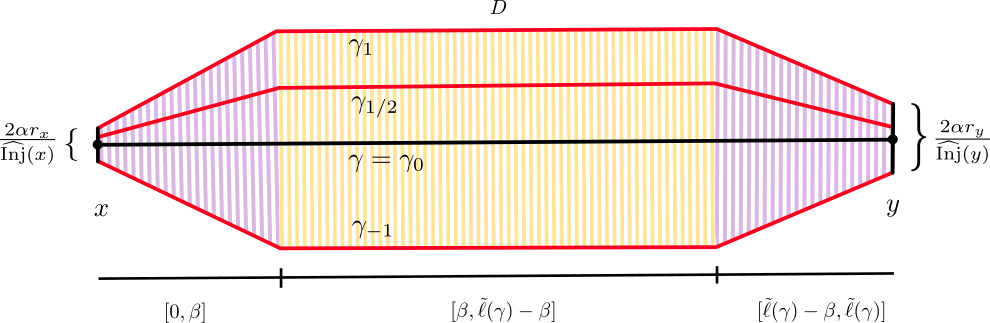
Figure 1: The domain $D$ as a subset of $\tilde{{S}}$. Note that the uniform thickness in the middle part is guaranteed by the injectivity radius lower bound of $\tilde{{S}}$. The paths $\gamma_{q}$ start start at distances in $[-\alpha r_{x}/\widehat{\mathrm{Inj}}\left({x}\right),\alpha r_{x}/\widehat{\mathrm{Inj}}\left({x}\right)]$ from $x$, fan out to a spread of $\alpha$, then fan back towards $y$.

Let $D=\{\gamma_{q}(t)\mid q\in[-1,1],t\in[0,\tilde{\ell}(\gamma)]\}$ be the colored region depicted in Fig. 1. Denote by $\mu$ the Riemannian area measure on $D$ according to the metric $\tilde{g}$, and by $\nu$ the measure on $D$ of $\gamma_{q}(t)$, obtained by taking $q$ to be a uniform random variable in $[-1,1]$ and $t$ an independent uniform random variable in $[0,\tilde{\ell}(\gamma)]$. Let $\rho:{\tilde{{S}}}\to[0,\infty)$ be a Borel measurable function. Integrating $\rho$ according to $\nu$, we have

$$\int_{D}\rho\leavevmode\nobreak\ d\nu=\frac{1}{2\tilde{\ell}(\gamma)}\int_{-1}^{1}\int_{0}^{\tilde{\ell}(\gamma)}\rho(\gamma_{q}(t))\leavevmode\nobreak\ dt\leavevmode\nobreak\ dq\,.$$

Thus, there exists a $q^{*}\in[-1,1]$ such that

$$\int_{0}^{\tilde{\ell}(\gamma)}\rho(\gamma_{q^{*}}(t))\leavevmode\nobreak\ dt\leq\tilde{\ell}(\gamma)\int_{D}\rho\leavevmode\nobreak\ d\nu\,.$$

By Item 4 of Proposition 12, we have that for every $q\in[-1,1]$,

$$\int_{\gamma_{q}}\rho\leavevmode\nobreak\ |d\tilde{z}|=\int_{0}^{\tilde{\ell}(\gamma)}\rho(\gamma_{q}(t))|\gamma_{q}^{\prime}(t)|\leavevmode\nobreak\ dt\lesssim\int_{0}^{\tilde{\ell}(\gamma)}\rho(\gamma_{q}(t))\leavevmode\nobreak\ dt\,$$

and so

$$\int_{\gamma_{q^{*}}}\rho\leavevmode\nobreak\ |d\tilde{z}|\lesssim\tilde{\ell}(\gamma)\int_{D}\rho\leavevmode\nobreak\ d\nu\,.$$

We bound $\int_{D}\rho\leavevmode\nobreak\ d\nu$ by comparing it to $\mu$ using the Cauchy-Schwarz inequality,

$$\int_{D}\rho\leavevmode\nobreak\ d\nu=\int_{D}\rho\frac{d\nu}{d\mu}\leavevmode\nobreak\ d\mu\leq\sqrt{\int_{D}\rho^{2}\leavevmode\nobreak\ d\mu}\leavevmode\nobreak\ \sqrt{\int_{D}\left(\frac{d\nu}{d\mu}\right)^{2}\leavevmode\nobreak\ d\mu}\,.$$

Since every curve $\gamma_{q}$ contains a curve in $\Gamma$, we obtain

$$\mathsf{EL}\left(\Gamma\right)=\sup_{\rho}\inf_{\eta\in\Gamma}\frac{L(\eta,\rho)^{2}}{\int_{D}\rho^{2}\leavevmode\nobreak\ d\mu}\leq\sup_{\rho}\inf_{q\in[-1,1]}\frac{\left(\int_{\gamma_{q}}\rho\leavevmode\nobreak\ |d\tilde{z}|\right)^{2}}{\int_{D}\rho^{2}\leavevmode\nobreak\ d\mu}\lesssim\tilde{\ell}(\gamma)^{2}\int_{D}\left(\frac{d\nu}{d\mu}\right)^{2}d\mu\,.$$ (11)

We now bound the Radon-Nikodym derivative in the right-hand side. For a point $z\in D$, the Radon-Nikodym derivative is given by

$$\frac{d\nu}{d\mu}(z)=\lim_{\varepsilon\to 0}\frac{\nu\left(B(z,\varepsilon)\right)}{\mu\left(B(z,\varepsilon)\right)}\asymp\lim_{\varepsilon\to 0}\frac{\mathrm{Leb}\left(\{(q,t)\in[-1,1]\times[0,\tilde{\ell}(\gamma)]\mid\gamma_{q}(t)\in B(z,\varepsilon)\}\right)}{2\tilde{\ell}(\gamma)\varepsilon^{2}}\,,$$ (12)

where we use the fact that $\mu(B(z,\varepsilon))\asymp\varepsilon^{2}$ since the curvature of ${\tilde{{S}}}$ is in $[-K_{1},K_{2}]$ (so for small enough $\varepsilon$, $\mu(B(z,\varepsilon))$ is larger than the area of a spherical cap of radius $\varepsilon$ on a sphere of radius $1/\sqrt{K_{2}}$, but smaller than the volume of a hyperbolic disc of curvature $-K_{1}$ of radius $\varepsilon$ (see e.g. [[]Theorems 11.14, 11.19]lee_introduction_to_riemannian_manifolds).

Claim 13.

Let $z_{1},z_{2}\in D$ have Fermi coordinates $(r_{1},t_{1})$ and $(r_{2},t_{2})$ with respect to $\gamma$ under the metric $\tilde{g}$. For any $\varepsilon>0$ small enough, if the distance between $z_{1}$ and $z_{2}$ is at most $\varepsilon$, then $|t_{1}-t_{2}|\lesssim\varepsilon$.

Proof.

Let $\eta:[0,\mathrm{dist}_{{\tilde{{S}}}}\left(z_{1},z_{2}\right)]\to{\tilde{{S}}}$ be a unit speed minimal geodesic from $z_{1}$ to $z_{2}$. As long as $\varepsilon>0$ is small, $B(z,\varepsilon)$ is convex so $\eta\subseteq B(z,\varepsilon)$. Denoting the Fermi coordinates of $\eta(s)$ by $(r(s),t(s))$, we have

$$\varepsilon \geq\mathrm{dist}_{{\tilde{{S}}}}\left(z_{1},z_{2}\right)=\int_{0}^{\mathrm{dist}_{{\tilde{{S}}}}\left(z_{1},z_{2}\right)}\sqrt{\left(\frac{dr}{ds}\right)^{2}+G(r(s),t(s))^{2}\left(\frac{dt}{ds}\right)^{2}}ds$$

$$\geq\int_{0}^{\mathrm{dist}_{{\tilde{{S}}}}\left(z_{1},z_{2}\right)}\cos(r(s)\sqrt{K_{2}})\frac{dt}{ds}ds\gtrsim|t_{2}-t_{1}|\,,$$

where the second inequality is by Item 4 of Proposition 12 and the last inequality is by (10). ∎

Let $t$ be such that there exists a $q\in[-1,1]$ with $\gamma_{q}(t)\in B(z,\varepsilon)$. For every such $t$, the curve $\eta_{t}:[-1,1]\to{\tilde{{S}}}$ given by $\eta_{t}(q)=\tilde{\varphi}_{\gamma}(q\cdot r(t),t)$ is a minimal geodesic with speed $r(t)$. Since it is minimal, the length of $\eta_{t}\cap B(z,\varepsilon)$ is bounded by $2\varepsilon$, and so the Lebesgue measure of all $q$ such that $\eta_{t}(q)\in B(z,\varepsilon)$ is bounded by $2\varepsilon/r(t)$. Denoting the Fermi coordinates of $z$ by $(r_{z},t_{z})$ in ${\tilde{{S}}}$ relative to $\gamma$, by 13 and the fact that $r(t)$ is continuous we have

$$\mathrm{Leb}\left(\{(q,t)\in[-1,1]\times[0,\tilde{\ell}(\gamma)]\mid\gamma_{q}(t)\in B(z,\varepsilon)\}\right)\lesssim\int_{t_{z}-C\varepsilon}^{t_{z}+C\varepsilon}\frac{\varepsilon}{r(t)}\leavevmode\nobreak\ dt\asymp\frac{\varepsilon^{2}}{r(t_{z})}\,.$$

Combining this with (11) and (12) and Item 4 of Proposition 12 we get

$$\mathsf{EL}\left(\Gamma\right) \lesssim\int_{D}\frac{1}{r(t_{z})^{2}}d\mu(z)\leq\int_{0}^{\tilde{\ell}(\gamma)}\int_{-r(t)}^{r(t)}\frac{1}{r(t)^{2}}\cosh(r(t)\sqrt{K_{1}})\leavevmode\nobreak\ ds\leavevmode\nobreak\ dt \lesssim\int_{0}^{\tilde{\ell}(\gamma)}\frac{1}{r(t)}\leavevmode\nobreak\ dt\,.$$ (13)

We partition the integral over $t$ into three parts as in the definition of $r(t)$, see Fig. 1. Firstly, when $t\in[\beta,\tilde{\ell}(\gamma)-\beta]$ we have that $r(t)=\alpha$, and so

$$\int_{\beta}^{\tilde{\ell}(\gamma)-\beta}\frac{1}{r(t)}\leavevmode\nobreak\ dt\lesssim\tilde{\ell}(\gamma)=\int_{\gamma}f(z)|dz|\asymp\mathrm{dist}_{w}\left(x,y\right)\,,$$ (14)

where we used the fact that $\gamma$ minimizes the distance in ${\tilde{{S}}}$ from $x$ to $y$ and that $f(z)\asymp\widehat{\mathrm{Inj}}\left({z}\right)^{-1}$. Secondly, when $t\in[0,\beta]$, we get

$$\int_{0}^{\beta}\frac{1}{r(t)}\leavevmode\nobreak\ dt=\int_{0}^{\beta}\frac{\alpha}{t/\beta+(1-t/\beta)\frac{r_{x}}{\widehat{\mathrm{Inj}}\left({x}\right)}}\leavevmode\nobreak\ dt=\frac{\alpha\beta\log\left(\frac{\widehat{\mathrm{Inj}}\left({x}\right)}{r_{x}}\right)}{1-\frac{r_{x}}{\widehat{\mathrm{Inj}}\left({x}\right)}}\lesssim\log\left(\frac{\widehat{\mathrm{Inj}}\left({x}\right)}{r_{x}}\right)\,,$$ (15)

since $r_{x}\leq\widehat{\mathrm{Inj}}\left({x}\right)/2$. A similar calculation shows that when $t\in[\tilde{\ell}(\gamma)-\beta,\tilde{\ell}(\gamma)]$, we have

$$\int_{\tilde{\ell}(\gamma)-\beta}^{\tilde{\ell}(\gamma)}\frac{1}{r(t)}\leavevmode\nobreak\ dt\asymp\log\left(\frac{\widehat{\mathrm{Inj}}\left({y}\right)}{r_{y}}\right)\,.$$ (16)

Combining (14), (15) and (16) into (13) proves the desired inequality. ∎

4 Proof of the eigenvalues lower bound

The goal of this section is to prove Theorem 1. For $\lambda>0$, define $N(\lambda)$ to be the number of eigenvalues in $(0,\lambda]$ of the Laplacian on ${S}$ . Our main goal is to show that there exists a universal constant $\Lambda_{0}>0$ such that $N(\lambda)\lesssim g\sqrt{\lambda I(S)}$ for all $\lambda\leq\Lambda_{0}$. Indeed, this would show that

$$\lambda_{k}\geq\frac{ck^{2}}{I(S)g^{2}}\,$$ (17)

for all $k$ such that $\frac{ck^{2}}{I(S)g^{2}}\leq\Lambda_{0}$. Since $I(S)\geq 1$, this condition holds when $k=1,\ldots,\lfloor g\sqrt{\Lambda_{0}/c}\rfloor$ so Theorem 1 then follows by decreasing the value $c$.

Let $\Lambda_{0}$ be a constant whose value is to be determined, fix $\lambda<\Lambda_{0}$, and let $\{\phi_{0},\phi_{1},\ldots\}$ be a smooth orthonormal basis of $L^{2}({S})$ where $\phi_{k}$ is a unit eigenvector of the Laplacian corresponding to $\lambda_{k}$ (see e.g. [[]Theorem 7.2.6]buser_book for the existence of such a basis). Define the function $e_{\lambda}:{S}^{2}\to\mathbb{R}$ by

$$e_{\lambda}(x,z)=\sum_{k\geq 1:\lambda_{k}\leq\lambda}\phi_{k}(x)\phi_{k}(z)\,;$$

the function $e_{\lambda}$ is called the spectral kernel. For $x\in{S}$, we define

$$\mu_{x}(\lambda)=e_{\lambda}(x,x)=\sum_{k\geq 1:\lambda_{k}\leq\lambda}\phi_{k}(x)^{2}\,,$$

and observe that

$$\int_{S}\mu_{x}(\lambda)\leavevmode\nobreak\ dx=N(\lambda)\,.$$ (18)

Hence, (17) would follow if we could show that $\mu_{x}(\lambda)\lesssim\sqrt{\lambda I(S)}$. However, unlike the case of a finite regular connected graph described in Section 1.1.1 (in which $\mu_{x}(\lambda)\lesssim\sqrt{\lambda}$) we cannot hope to bound $\mu_{x}(\lambda)$ uniformly in $x$. Thus, our goal is to bound $\mu_{x}(\lambda)$ for each $x\in{S}$ separately.

For $x$ with $\mu_{x}>0$, define the function $f_{x}:{S}\to\mathbb{R}$ by

$$f_{x}(z)=\frac{e_{\lambda}(x,z)}{\sqrt{\mu_{x}(\lambda)}}\,,$$

and observe that $f_{x}(x)=\sqrt{\mu_{x}(\lambda)}$ and that

$$\|f_{x}\|_{2}^{2}=\frac{\int_{S}e_{\lambda}(x,z)^{2}\leavevmode\nobreak\ dz}{\mu_{x}(\lambda)}=\frac{\int_{S}\left(\sum_{k\geq 1:\lambda_{k}\leq\lambda}\phi_{k}(x)\cdot\phi_{k}(z)\right)^{2}\leavevmode\nobreak\ dz}{\mu_{x}(\lambda)}=\frac{\mu_{x}(\lambda)}{\mu_{x}(\lambda)}=1\,.$$ (19)

We will require an upper bound on the gradient of $f$ similar to Bernstein inequalities for Laplacian eigenfunctions. We will use the following bound on the gradient of $f_{x}$; it follows from known methods (such as [OP13]) but we were unable to find a reference that implies it, therefore we provide its short proof in Section 4.2.

Lemma 14.

For all $z\in{S}$ we have

$$|\nabla f_{x}(z)|\lesssim e^{2\sqrt{\lambda}}\widehat{\mathrm{Inj}}\left({z}\right)^{-1}\,.$$

Recall Definition 4 for the weighted distance $\mathrm{dist}_{w}\left(\cdot,\cdot\right)$, and for any $x\in{S}$ and $R>0$ let

$$B_{w}\left(x,R\right)=\{y\in{S}\mid\mathrm{dist}_{w}\left(x,y\right)\leq R\}\,.$$

Lemma 15.

Let $R\geq 1$ and $x\in{S}$. Suppose that either $\mathrm{Vol}(B_{w}\left(x,R\right))\geq\frac{16}{\mu_{x}(\lambda)}$ or $B_{w}\left(x,R\right)={S}$. Then

$$\mu_{x}(\lambda)\lesssim\lambda\Big{(}R+\log\big{(}\frac{1}{\mu_{x}(\lambda)\wedge 1}\big{)}\Big{)}\,.$$

Proof.

We first find a point $y\in B_{w}\left(x,R\right)$ such that $f_{x}(y)\leq\frac{1}{4}f_{x}(x)$. Indeed, if $B_{w}\left(x,R\right)={S}$, then it is immediate that there exists $y\in B_{w}\left(x,R\right)$ with $f_{x}(y)=0$ since $\int_{y}f_{x}(y)d{S}=0$. Otherwise, we have that

$$\mathrm{Vol}\big{(}\{z\in{S}\mid f_{x}(z)>\frac{1}{4}f_{x}(x)\}\big{)}<\frac{||f_{x}||^{2}}{f_{x}(x)^{2}/16}=\frac{16}{\mu_{x}(\lambda)}\,,$$ (20)

hence in the case $\mathrm{Vol}(B_{w}\left(x,R\right))\geq\frac{16}{\mu_{x}(\lambda)}$ we again obtain such a point $y$.

Next, using Lemma 14 we can choose a universal constant $c>0$ small enough so that setting

$$r_{x}=c(f_{x}(x)\wedge 1)\widehat{\mathrm{Inj}}\left({x}\right)\,,\quad r_{y}=c(f_{x}(x)\wedge 1)\widehat{\mathrm{Inj}}\left({y}\right)\,,$$

and since $\lambda<\Lambda_{0}$ is bounded from above, this yields that

$$\inf\{f_{x}(z):z\in B(x,r_{x})\}\geq{3f_{x}(x)/4}\,,$$

and

$$\sup\{f_{x}(z):z\in B(y,r_{y})\}\leq f_{x}(x)/2\,.$$

In particular, the balls $B(x,r_{x})$ and $B(y,r_{y})$ are disjoint. Let $\Gamma$ denote the set of all rectifiable curves between the boundaries of the balls which do not enter the balls. Theorem 5 states that

$$\mathsf{EL}\left(\Gamma\right)\lesssim R+\log\left(\frac{1}{c(f_{x}(x)\wedge 1)}\right)\,.$$

It is well known that given two disjoint open sets $A$ and $B$ of ${S}$, the extremal length of the family of curves connecting $\partial A$ and $\partial B$ in ${S}\setminus(A\cup B)$ is the inverse of the Dirichlet energy $\int_{S}|\nabla f|^{2}$ of the unique harmonic function $f$ in ${S}\setminus(A\cup B)$ taking $1$ on $\partial A$ and $0$ on $\partial B$, see [MR66, Lemma III1.1, p250]. Since harmonic functions minimize the Dirichlet energy, after rescaling the boundary values we obtain that

$$\int_{S}|\nabla f_{x}(z)|^{2}\leavevmode\nobreak\ dz\geq\frac{f_{x}(x)^{2}/16}{\mathsf{EL}\left(\Gamma\right)}\gtrsim\frac{f_{x}(x)^{2}}{R+\log(\frac{1}{c(f_{x}(x)\wedge 1)})}\,.$$ (21)

Note that we have used [MR66, Lemma III1.1, p250] with the level sets $\{z:f_{x}(z)\leq f_{x}(x)/2\}$ and $\{z:f_{x}(z)\geq 3f_{x}(x)/4\}$ taking the role of $A$ and $B$ above and used a trivial monotonicity of the Dirichlet energy. Since $f_{x}$ is a linear combination of eigenfunctions with corresponding eigenvalues at most $\lambda$ we may bound

$$\lambda\geq\left<\Delta f_{x},f_{x}\right>=\left<\nabla f_{x},\nabla f_{x}\right>=\int_{S}|\nabla f_{x}(z)|^{2}\leavevmode\nobreak\ dz\,.$$

We put this and $f_{x}(x)^{2}=\mu_{x}(\lambda)$ in (21) and obtain that

$$\mu_{x}(\lambda)\lesssim\lambda\Big{(}R+\log\big{(}\frac{1}{\mu_{x}(\lambda)\wedge 1}\big{)}\Big{)}\,.$$

∎

Lemma 16.

Let $x\in{S}$ and $R\geq 1$ be such that $B_{w}\left(x,R\right)\neq{S}$. Then

$$\int_{B_{w}\left(x,R\right)}\frac{1}{\widehat{\mathrm{Inj}}\left({z}\right)^{2}}\leavevmode\nobreak\ dz\gtrsim R\,.$$

Proof.

Since $B_{w}\left(x,R\right)\neq{S}$ the boundary $\partial B_{w}\left(x,R\right)$ is non-empty. Let $y$ be a point in $\partial B_{w}\left(x,R\right)$ which minimizes the original distance $\mathrm{dist}_{{S}}\left(x,y\right)$. We denote by $\gamma$ a minimal geodesic in ${S}$ between $x$ and $y$, which, by our choice of $y$, is contained in $B_{w}\left(x,R\right)$.

We proceed by analyzing two cases. First, if $\ell=\mathrm{dist}_{{S}}\left(x,y\right)\leq 1$, then all points $z\in B_{S}(x,\ell)$ have $\widehat{\mathrm{Inj}}\left({z}\right)\asymp\widehat{\mathrm{Inj}}\left({x}\right)$ uniformly by Lemma 10. Since $y\in\partial B_{w}\left(x,R\right)$ we must have that $w\left(\gamma\right)\geq R$, hence $\widehat{\mathrm{Inj}}\left({x}\right)^{-1}\gtrsim R/\ell$. We get

$$\int_{B_{w}\left(x,R\right)}\frac{1}{\widehat{\mathrm{Inj}}\left({z}\right)^{2}}\leavevmode\nobreak\ dz\geq\int_{B_{S}(x,\ell)}\frac{1}{\widehat{\mathrm{Inj}}\left({z}\right)^{2}}\leavevmode\nobreak\ dz\gtrsim\frac{\ell^{2}}{\widehat{\mathrm{Inj}}\left({x}\right)^{2}}\gtrsim R^{2}\geq R\,,$$

where the first and last inequalities are since $R\geq 1$.

Next we handle the case in which $\ell>1$. Let $c\in(0,1/4)$ be a small universal constant that will be chosen later. Parameterizing $\gamma$ by length, we first note that for any $t\in[0,\ell-c]$ we must have

$$B_{S}(\gamma(t),c\widehat{\mathrm{Inj}}\left({\gamma(t)}\right))\subseteq B_{w}\left(x,R\right)\,,$$ (22)

since otherwise the ball $B_{S}(\gamma(t),c\widehat{\mathrm{Inj}}\left({\gamma(t)}\right))$ contains some other point of $\partial B_{w}(x,R)$ which we can connect to $\gamma(t)$ in a path of length at most $c$, contradicting the minimality of $\ell$.

Consider the set $D=\{(t,r):t\in[0,\ell-c],|r|\leq c\widehat{\mathrm{Inj}}\left({\gamma(t)}\right)\}$ which is a subset of $D_{\gamma}$ defined above Proposition 11. Since $\gamma$ is a unit speed minimal geodesic connecting two points, Proposition 11 implies that the Fermi coordinate map $\varphi_{\gamma}$ is one-to-one. By (22) we have $\varphi_{\gamma}(D)\subseteq B_{w}(x,R)$ so

$$\int_{B_{w}\left(x,R\right)}\frac{1}{\widehat{\mathrm{Inj}}\left({z}\right)^{2}}\leavevmode\nobreak\ dz \geq \int_{\varphi_{\gamma}(D)}\frac{1}{\widehat{\mathrm{Inj}}\left({z}\right)^{2}}\leavevmode\nobreak\ dz=\int_{0}^{\ell-c}\int_{-c\widehat{\mathrm{Inj}}\left({\gamma(t)}\right)}^{c\widehat{\mathrm{Inj}}\left({\gamma(t)}\right)}\frac{1}{\widehat{\mathrm{Inj}}\left({\varphi_{\gamma}(t,r)}\right)^{2}}\cosh(r)drdt$$ (23)

$$\gtrsim \int_{0}^{\ell-c}\frac{c}{\widehat{\mathrm{Inj}}\left({\gamma(t)}\right)}dt=c\cdot\left(w\left(\gamma\right)-w\left(\gamma[0,\ell-c]\right)\right)\,.$$

where we used (7) and the fact that $\widehat{\mathrm{Inj}}\left({\varphi_{\gamma}(t,r)}\right)\asymp\widehat{\mathrm{Inj}}\left({\gamma(t)}\right)$.

We argue that if $z\in B_{w}\left(x,R\right)$ and $d_{S}(x,z)\geq 1/2$, then $\mathrm{Inj}\left(z\right)\geq{\varepsilon/R}$ for some constant $\varepsilon>0$. Otherwise, by Lemma 10, any curve connecting $x$ to $z$, just by considering its last tip of length $1/2$, must have weight $\gtrsim\widehat{\mathrm{Inj}}\left({z}\right)^{-1}\geq R/\varepsilon$, which is a contradiction for $\varepsilon>0$ small enough.

We apply this with $z=\gamma(\ell-c)$ and obtain that $\mathrm{Inj}\left(\gamma(\ell-c)\right)\geq\sqrt{c}/R$ as long as $c>0$ is small enough. By Lemma 10 we have $\mathrm{Inj}\left(\gamma(t)\right)\gtrsim\sqrt{c}/R$ for all $t\in[\ell-c,\ell]$. We deduce that $w\left(\gamma[\ell-c,\ell]\right)\lesssim\sqrt{c}R$, which together with (23) and that $w\left(\gamma\right)\geq R$ gives

$$\int_{B_{w}\left(x,R\right)}\frac{1}{\widehat{\mathrm{Inj}}\left({z}\right)^{2}}\leavevmode\nobreak\ dz\gtrsim c(w\left(\gamma\right)-w\left(\gamma[\ell-c,\ell]\right))\gtrsim c\left(R-\sqrt{c}R\right)\gtrsim R\,,$$

concluding the proof. ∎

Lemma 17.

For every $\varepsilon\in(0,1)$ and $R\geq 1$, let

$$A_{R,\varepsilon}=\{x\in{S}\mid\mathrm{Vol}\left(B_{w}\left(x,R\right)\right)<\varepsilon R\textrm{ and }B_{w}\left(x,R\right)\neq{S}\}\,.$$

Then

$$\mathrm{Vol}\left(A_{R,\varepsilon}\right)\lesssim\varepsilon I({S})\mathrm{Vol}({S})\,.$$

Proof.

Let $x_{1},\ldots,x_{k}$ be a maximal set of points in $A_{R,\varepsilon}$ such that the interiors of $B_{w}\left(x_{i},R/2\right)$ are pairwise disjoint. By maximality, for every $x\in A_{R,\varepsilon}$ the set $B_{w}\left(x,R/2\right)$ intersects some $B_{w}\left(x_{i},R/2\right)$, so the triangle inequality implies that $\mathrm{dist}_{w}\left(x,x_{i}\right)\leq R$ and we deduce that the balls $\{B_{w}\left(x_{i},R\right)\}_{i=1}^{k}$ cover $A_{R,\varepsilon}$. As the volume of each ball is at most $\varepsilon R$, we have that

$$\varepsilon Rk\geq\mathrm{Vol}(A_{R,\varepsilon})\,.$$ (24)

On the other hand,

$$\mathrm{Vol}({S})\cdot I({S})=\int_{{S}}\frac{1}{\widehat{\mathrm{Inj}}\left({z}\right)^{2}}\leavevmode\nobreak\ dz\geq\sum_{i=1}^{k}\int_{B_{w}\left(x_{i},R/2\right)}\frac{1}{\widehat{\mathrm{Inj}}\left({z}\right)^{2}}\leavevmode\nobreak\ dz\quad\gtrsim\quad kR,$$

by Lemma 16. This gives the desired result. ∎

4.1 Proof of Theorem 1

For each $j\geq 0$ we set the numbers

$$\mu_{j}=2^{j}\sqrt{\lambda I(S)}\,,\qquad R_{j}=c2^{j}\sqrt{\frac{I(S)}{\lambda}}=c\mu_{j}/\lambda\,,$$

where $c>0$ is a small constant which will be chosen later. We take $\Lambda_{0}$ to be small enough so that $R_{0}\geq 1$ for all $\lambda<\Lambda_{0}$. We further set

$$G_{0}=\{\ x\in{S}\mid 0<\mu_{x}(\lambda)\leq\mu_{0}\}\,,$$

and for every integer $j\geq 1$,

$$G_{j}=\{\ x\in{S}\mid\mu_{j-1}<\mu_{x}(\lambda)\leq\mu_{j}\}\,.$$

We proceed by bounding $\mathrm{Vol}(G_{j})$ from above. If $x\in G_{j}$ we obtain by Lemma 15 that either $\mathrm{Vol}(B_{w}\left(x,R_{j}\right))\leq 32/\mu_{j}$ and $B_{w}\left(x,R_{j}\right)\neq{S}$ or that

$$\mu_{j}\lesssim\lambda R_{j}+\lambda\log(1/(\frac{\mu_{j}}{2}\wedge 1))\lesssim\lambda R_{j}+\lambda(\mu_{j}\wedge 1)^{-1/2}\,.$$ (25)

The first term on the right-hand side is equal to $c\mu_{j}$, and cannot be $\gtrsim\mu_{j}$ for $c$ small enough. The second term on the right-hand side is bounded above by $\lambda^{3/4}$ since $\mu_{j}\geq\mu_{0}\geq\sqrt{\lambda}$, hence it also cannot be greater than $\mu_{j}$ as long as $\Lambda_{0}$ is small enough. Thus $\mathrm{Vol}(B_{w}\left(x,R_{j}\right))\leq 32/\mu_{j}$ and $B_{w}\left(x,R_{j}\right)\neq{S}$. By Lemma 17 with $\varepsilon=\frac{32}{\mu_{j}R_{j}}=\frac{32}{c4^{j}I(S)}$, we get

$$\mathrm{Vol}(G_{j})\lesssim 4^{-j}\mathrm{Vol}({S})\,.$$ (26)

We put this in (18), giving

$$N(\lambda)=\int_{S}\mu_{x}(\lambda)\leavevmode\nobreak\ dx\leq\sum_{j\geq 0}\mu_{j}\mathrm{Vol}(G_{j})\lesssim\sum_{j\geq 0}2^{-j}\sqrt{\lambda I(S)}\,,$$ (27)

which implies (17) and concludes the proof. ∎

4.2 Proof of the gradient upper bound

Proof of Lemma 14.

We follow the harmonic extension method of [[]Section 3]ortega_pridhnani_gradient_bound. Let $\phi_{0},\phi_{1},\ldots\ \phi_{k}$ be the orthonormal eigenvectors of the Laplacian with eigenvalue smaller than or equal to $\lambda$ (as described in the beginning of this section). Then $f_{x}$ can be written as the linear combination $f_{x}(z)=\sum_{i=1}^{k}\beta_{i}\phi_{i}(z)$, with $\beta_{i}=\phi_{i}(x)/\sqrt{\mu_{x}(\lambda)}$. Let $h(z,t)$ be the harmonic extension of $f_{x}$ to the manifold $M={S}\times\mathbb{R}$, i.e.

$$h(z,t)=\sum_{i=1}^{k}\beta_{i}\phi_{i}(z)e^{\sqrt{\lambda_{i}}t}\,.$$

Observe that $\nabla h(z,0)$ agrees with $\nabla f_{x}$ on the coordinates corresponding to ${S}$, and has an additional coordinate equal to $\sum_{i=1}^{k}\beta_{i}\phi_{i}(z)\sqrt{\lambda_{i}}$. Thus, $|\nabla f_{x}(z)|^{2}\leq|\nabla h(z,0)|^{2}$. Since $h$ is harmonic, by a classical theorem of Schoen and Yau ([[]Corollary 3.2, p21]Schoen_Yau_Book with $K=1$ and $a=1$, see also (3.3) in [OP13]) we have

$$|\nabla h(z,0)|^{2}\leq C\sup\{h(y)^{2}\mid y\in{B_{M}\left((z,0),1\right)}\}\,.$$

Suppose that the supremum is attained at the point $(z^{*},t^{*})\in B_{M}\left((z,0),1\right)$. Since $h$ is harmonic, $h^{2}$ is subharmonic, and for all $r<\mathrm{Inj}\left((z^{*},t^{*}),M\right)$ we have by [[]Theorem 6.2, p77]Schoen_Yau_Book that

$$h(z^{*},t^{*})^{2}\leq\frac{1}{\mathrm{Vol}\left(B_{M}\left((z^{*},t^{*}),r\right)\right)}\int_{B_{M}\left((z^{*},t^{*}),r\right)}h(y)^{2}\leavevmode\nobreak\ dM\,.$$ (28)

By the triangle inequality, the ball $B_{M}\left((z^{*},t^{*}),r\right)$ contains the set $B_{S}(z^{*},r/2)\times[t^{*}-r/2,t^{*}+r/2]$, thus, its volume is at least $4\pi\sinh(r/2)^{2}\cdot r/2\gtrsim r^{3}$. Together with (28), this gives

$$|\nabla f_{x}(z)|^{2}\lesssim\frac{1}{r^{3}}\int_{B_{M}\left((z^{*},t^{*}),r\right)}h(y)^{2}dy\,.$$ (29)

Now take $r=\min\{1,\mathrm{Inj}\left((z^{*},t^{*}),M\right)\}=\widehat{\mathrm{Inj}}\left({z^{*}}\right)$. By Lemma 10, since $\mathrm{dist}_{{S}}\left(z^{*},z\right)\leq 1$, we have $\widehat{\mathrm{Inj}}\left({z}\right)^{-1}\asymp\widehat{\mathrm{Inj}}\left({z^{*}}\right)^{-1}$, and so $1/r\asymp\widehat{\mathrm{Inj}}\left({z}\right)^{-1}$. To bound the integral, observe that $B_{M}\left((z^{*},t^{*}),r\right)\subseteq{S}\times[t^{*}-r,t^{*}+r]$. We then have

$$\int_{B_{M}\left((z^{*},t^{*}),r\right)}h(y)^{2}\leavevmode\nobreak\ dM \leq\int_{t^{*}-r}^{t^{*}+r}\int_{S}h(z,t)^{2}\leavevmode\nobreak\ dzdt$$

$$=\int_{t^{*}-r}^{t^{*}+r}\int_{S}\left(\sum_{i=1}^{k}\beta_{i}\phi_{i}(z)e^{\sqrt{\lambda_{i}}t}\right)^{2}\leavevmode\nobreak\ dzdt$$

$$=\int_{t^{*}-r}^{t^{*}+r}\sum_{i=1}^{k}\beta_{i}^{2}e^{2\sqrt{\lambda_{i}}t}dt$$

$$\leq 2re^{4\sqrt{\lambda}}\sum_{i=1}^{k}\beta_{i}^{2}=2re^{4\sqrt{\lambda}}\|f\|_{2}^{2}=2re^{4\sqrt{\lambda}}\,,$$

where the last equality is due to (19). Using (29) we deduce that

$$|\nabla f_{x}(z)|\lesssim e^{2\sqrt{\lambda}}r^{-1}\lesssim e^{2\sqrt{\lambda}}\widehat{\mathrm{Inj}}\left({z}\right)^{-1}\,$$

as needed. ∎

5 Heat kernel bound

The goal of this section is to prove Theorem 2. Let $\gamma_{1},\ldots,\gamma_{s}$ be the set of all simple closed geodesics of length $\leq 2\sinh^{-1}(1)$ and let $C(\gamma_{i})$ be their collars, as described in Lemma 7. It will be convenient to chop off the parts of the collar at distance at most $1$ to its boundary, that is, we define $\tilde{C}(\gamma_{i}):=\{x\in C(\gamma_{i})\mid\mathrm{dist}(x,\partial C(\gamma_{i}))\geq 1\}$.

Let ${{S}}^{\mathrm{thin}}:=\cup_{i}\{\tilde{C}(\gamma_{i})\}$ and ${{S}}^{\mathrm{thick}}:={S}\backslash{{S}}^{\mathrm{thin}}$. By Lemma 7 we have that $\mathrm{Inj}\left(x\right)\gtrsim 1$ for every $x\in{{S}}^{\mathrm{thick}}$ and $\mathrm{Inj}\left(x\right)\lesssim 1$ for every $x\in{{S}}^{\mathrm{thin}}$.

Proposition 18.

For any $x\in{{S}}^{\mathrm{thick}}$ and any $t\in[1/2,1]$ we have

$$p_{t}^{{S}}(x,x)\lesssim p_{t}^{{\mathbb{H}}}(0,0)+1\,.$$

Proof.

For a hyperbolic surface ${S}$, recall that the heat kernel $p_{t}^{{S}}(x,y)$ is given by $p_{t}^{{S}}(x,y)=\sum_{T\in\Gamma}p_{t}^{{\mathbb{H}}}(\tilde{x},T\tilde{y})$, where $\Gamma$ is a group red of isometries acting on ${\mathbb{H}}$ so that ${S}=\Gamma\backslash{\mathbb{H}}$, and $\tilde{x}$ and $\tilde{y}$ are arbitrary inverse images of $x$ and $y$ of the projection to ${S}$. To estimate $p_{t}^{{S}}(x,x)$, we partition the group translations by distance of $T\tilde{x}$ from $\tilde{x}$. Denoting

$$\Gamma(m):=\{T\in\Gamma\mid m<d_{\mathbb{H}}(\tilde{x},T\tilde{x})\leq m+1\}\,,$$

we have

$$p_{t}^{{S}}(x,x) =p_{t}^{{\mathbb{H}}}(0,0)+\sum_{m=0}^{\infty}\sum_{T\in\Gamma(m)}p_{t}^{{\mathbb{H}}}(\tilde{x},T\tilde{x})\,.$$ (30)

We bound $|\Gamma(m)|$ by an explicit version of [[]Lemma 7.5.3]buser_book. Let $D$ be the disc around $\tilde{x}$ of radius $\mathrm{Inj}\left(x\right)$. Every disc $T(D)$ with $T\in\Gamma(m)$ is contained in the disc of radius $m+1+\mathrm{Inj}\left(x\right)$ around $\tilde{x}$ in ${\mathbb{H}}$ which has volume $2\pi\left(\cosh(m+1+\mathrm{Inj}\left(x\right))-1\right)\leq 2\pi e^{m+1+\mathrm{Inj}\left(x\right)}$. On the other hand, the volume of $T(D)$ is $2\pi\left(\cosh(\mathrm{Inj}\left(x\right))-1\right)$ and $\{T(D)\}_{T\in\Gamma(m)}$ are non-intersecting. Thus,

$$\#\Gamma(m)\leq\frac{e^{\mathrm{Inj}\left(x\right)+1}}{\cosh(\mathrm{Inj}\left(x\right))-1}e^{m}\lesssim\left(1+\frac{1}{\mathrm{Inj}\left(x\right)^{2}}\right)e^{m}\lesssim e^{m}\,.$$ (31)

where in the second inequality we relied on the asymptotics of the function $\cosh(r)$ for $r\to 0$ and $r\to\infty$, and in the third inequality we relied on our assumption that $x\in{{S}}^{\mathrm{thick}}$. Next, a well-known bound on $p_{t}^{{\mathbb{H}}}$ (see [[]Lemma 7.4.26]buser_book) states that

$$p_{t}^{{\mathbb{H}}}(x,y)\lesssim\frac{1}{t}\exp\left(-{\frac{{d_{\mathbb{H}}(x,y)}^{2}}{8t}}\right)\,.$$ (32)

We use this to bound the sum on the right hand side of (30) by

$$\sum_{m=1}^{\infty}\sum_{T\in\Gamma(m)}p_{t}^{{\mathbb{H}}}(\tilde{x},T\tilde{x})\lesssim\frac{1}{t}\sum_{m=1}^{\infty}\exp\left(m-m^{2}/8t\right)\lesssim 1\,,$$

since the term over $m$ is convergent. For the sum over $T\in\Gamma(0)$ we note that $d_{{\mathbb{H}}}(\tilde{x},T\tilde{x})\geq\mathrm{Inj}\left(x\right)\gtrsim 1$ for every $T\in\Gamma(0)$ so by (32) we obtain a contribution of another constant. ∎

We next bound the behavior of $p_{t}^{{S}}(x,x)$ in the thin part.

Proposition 19.

Let $\gamma$ be a simple closed geodesic of length $\ell\leq 2\sinh^{-1}(1)$. Then for any $t\in[1/2,1]$ we have

$$\int_{\tilde{C}(\gamma)}p_{t}^{{S}}(x,x)\leavevmode\nobreak\ dx\lesssim\log(1/\ell)\,.$$ (33)

Proof.

We apply the classical Li and Yau theorem (see Corollary 3.1 in [LY86] with $\alpha=3/2$ and $\varepsilon=1/2$) which asserts that if ${S}$ is a complete Riemannian manifold without boundary and with Ricci curvature bounded from below by $-K$, then

$$p_{t}^{{S}}(x,y)\lesssim\mathrm{Vol}(B(x,\sqrt{t}))^{-1/2}\mathrm{Vol}(B(y,\sqrt{t}))^{-1/2}\exp\left(CKt-\frac{d_{{S}}(x,y)^{2}}{4.5t}\right)\,,$$ (34)

where $C<\infty$ is a universal constant. Using the above bound yields

$$p_{t}^{{S}}(x,x)\lesssim\frac{1}{\mathrm{Vol}(B(x,\sqrt{t}))}\,,$$ (35)

as long as $t\leq 1$. Let $x\in\tilde{C}(\gamma)$ have Fermi coordinates $(\rho,\theta)$ relative to $\gamma$, where $\rho\geq 0$ without loss of generality. The ball $B(x,\sqrt{t})$ is contained in the collar $C(\gamma)$. Hence, if we let $\eta$ be the unit-speed geodesic given by $\eta(s)=\varphi_{\gamma}(\rho+s,\theta)$ with $s\in[0,\sqrt{t}/2]$ (that is, $\eta$ extends outwards from $x$, is perpendicular to $\gamma$ has length $\sqrt{t}/2$), then $B(x,\sqrt{t})$ contains the tubular neighborhood of $\eta$ given by $\varphi_{\eta}([0,\sqrt{t}/2]\times[0,r])$ where $r\asymp\mathrm{Inj}\left(x\right)$ (which is possible since $\mathrm{Inj}\left(x\right)\lesssim 1$). We thus obtain that $\mathrm{Vol}(B(x,\sqrt{t}))\gtrsim\mathrm{Inj}\left(x\right)$. Plugging this into above volume estimate into the Li-Yau bound (35), by Proposition 8 we thus obtain

$$\int_{\tilde{C}(\gamma)}p_{t}^{{S}}(x,x)\leavevmode\nobreak\ dx \lesssim\int_{0}^{2\pi}\int_{0}^{W(\ell)}\frac{1}{\mathrm{Inj}\left(x\right)}\ell\cosh(\rho)\leavevmode\nobreak\ d\rho d\theta\lesssim W(\ell)\lesssim\log(1/\ell)\,.$$

∎

5.1 Proof of Theorem 2

It is well known that $p_{t}(x,x)\geq 1/\mathrm{Vol}(S)$ so the expression in the absolute value is always non-negative. By the spectral theorem [[]Section VI.1, Sturm-Liouville decomposition]chavel_book,

$$\int_{{S}}\Big{[}p_{t}^{{S}}(x,x)-\frac{1}{\mathrm{Vol}({S})}\Big{]}\leavevmode\nobreak\ dx=\sum_{k=1}^{\infty}e^{-t\lambda_{k}}=\sum_{k=1}^{2g-3}e^{-t\lambda_{k}}+\sum_{k=2g-2}^{\infty}e^{-t\lambda_{k}}\,.$$ (36)

Applying Theorem 1 and recalling that $g\asymp\mathrm{Vol}({S})$ we bound the first sum on the right-hand side by

$$\sum_{k=1}^{2g-3}e^{-t\lambda_{k}}\leq\sum_{k=1}^{\infty}e^{-ct\frac{k^{2}}{I({S})\mathrm{Vol}({S})^{2}}}\lesssim\int_{0}^{\infty}\exp\left(-ct\frac{x^{2}}{I({S})\mathrm{Vol}({S})^{2}}\right)dx\asymp\mathrm{Vol}({S})\sqrt{\frac{I({S})}{t}}\,.$$ (37)

For the second sum on the right-hand side, a result by Otal and Rosas [[]Theorem 1]otal_rosas_eigenvalues_must_be_large states that $\lambda_{2g-2}>\frac{1}{4}$. Denoting $t=\tau+1/2$ for $\tau\geq 1/2$, we get

$$\sum_{k=2g-2}^{\infty}e^{-t\lambda_{k}}=\sum_{k=2g-2}^{\infty}e^{-(\tau+1/2)\lambda_{k}}\leq e^{-\tau/4}\sum_{k=0}^{\infty}e^{-\frac{1}{2}\lambda_{k}}\lesssim e^{-t/4}\int_{{S}}p_{1/2}^{{S}}(x,x)\leavevmode\nobreak\ dx\,.$$

Let $\gamma_{1},\ldots,\gamma_{s}$ be the set of all simple closed geodesics of length $\leq 2\sinh^{-1}(1)$ in ${S}$. We appeal to Proposition 18 and Proposition 19 with $t=1/2$; since $p_{1/2}^{{\mathbb{H}}}(0,0)\asymp 1$, we get

$$\int_{{S}}p_{1/2}^{{S}}(x,x)\leavevmode\nobreak\ dx \lesssim\mathrm{Vol}({S})+\sum_{i=1}^{s}\log\left(\frac{1}{\ell(\gamma_{i})}\right)\lesssim\mathrm{Vol}({S})\sqrt{I({S})}\,,$$

since $\sum_{i=1}^{s}\log(1/\ell(\gamma_{i}))\lesssim\sum_{i=1}^{s}\ell(\gamma_{i})^{-1/2}$ which by Cauchy-Schwartz is at most $\sqrt{s\sum_{i=1}^{s}\ell(\gamma_{i})^{-1}}$ and we get the above inequality using Corollary 9. All this gives that

$$\sum_{k=2g-2}^{\infty}e^{-t\lambda_{k}}\lesssim e^{-t/4}\mathrm{Vol}({S})\sqrt{I({S})}\,,$$

which together with (36) and (37) concludes the proof. ∎

Remark 20.

The choice of $t=1$ in Theorem 2 is arbitrary since it is the large values of $t$ that are interesting. The same proof shows that for any $t_{0}>0$ there exists $C(t_{0})<\infty$ such that (2) holds for all $t\geq t_{0}$ and $C=C(t_{0})$.

6 Sharpness

Let $I\geq 1$ be real and $g\geq 2$ be an integer. Set $\varepsilon=\min\{\frac{1}{I},\sinh^{-1}(1)\}$ and $n=g-1$. Let $Y$ be a pair of pants with boundary geodesics of lengths $(1,1,\varepsilon)$, and let $X$ be the surface obtained by gluing two identical copies of $Y$ along their two boundary geodesics of length $1$, without twists. Note that $X$ has two boundary components, each of length $\varepsilon$. Finally, let ${S}$ be the surface of genus $g$ obtained by gluing together without twists $n$ copies of $X$ in a cycle. See Fig. 2.

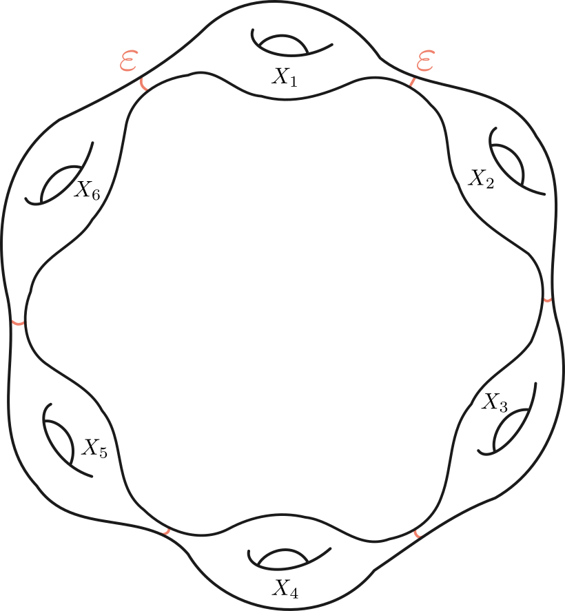
Figure 2: A schematic of $S$ for $n=6$.

It is straightforward to check that $I({S})\asymp 1/\varepsilon$, and so $I({S})\gtrsim I$. We claim that the eigenvalues of the Laplacian on ${S}$ satisfy

$$\lambda_{k}\leq\frac{C\varepsilon k^{2}}{g^{2}}\,,$$

where $k\in\{1,\ldots,n\}$ and $C<\infty$ is a universal constant. We will do this by constructing appropriate test functions for the minimax principle.

Let $k\leq n$ be fixed. Consider $k$ disjoint connected subsets ${S}_{1},\ldots,{S}_{k}$ of ${S}$, where each ${S}_{i}$ is a concatenation of $\lfloor\frac{n}{k}\rfloor$ consecutive copies of X. We assume for simplicity that $\lfloor\frac{n}{k}\rfloor$ is odd and write $\lfloor\frac{n}{k}\rfloor=2m+1$; the even case is handled similarly. For each $i$ we define a function $f_{i}(x)$ whose support is ${S}_{i}$, so that the functions $\{f_{i}\}_{i=1}^{k}$ have disjoint supports. Let us describe $f_{1}$; the other functions are constructed similarly. Assume that $S_{1}$ is the concatenation of $X_{1},\ldots,X_{2m+1}$. If $x\in X_{j}$ for some $j\in\{1,\ldots,2m+1\}$ and $\mathrm{dist}\left(x,\partial X_{j}\right)\geq 1$, then we set $f_{1}(x)=\frac{j}{m+1}$ if $j\leq m+1$ and $f_{1}(x)=1-\frac{j-(m+1)}{m+1}$ if $j>m+1$. When $\mathrm{dist}\left(x,\partial X_{j}\right)<1$, we set the values of $f_{i}$ so that they interpolate linearly between the two values in the boundary $\{x:\mathrm{dist}\left(x,\partial X_{j}\right)=1\}$.

It is straightforward to verify that $\|f_{i}\|_{2}\asymp\sqrt{m}$ and $\int_{S}|\nabla f_{i}|^{2}\leavevmode\nobreak\ d{S}\lesssim\varepsilon/m$. The functions $\{f_{i}\}$ are not smooth, but one can easily make them smooth (say, by mollifying, as we did in (8)) and still have the same bounds on the norm and the Dirichlet energy as above. Thus, the minimax principle [[]Theorem 8.2.1 (i)]buser_book and the fact that $m\asymp n/k$ gives that $\lambda_{k}\lesssim\varepsilon k^{2}/n^{2}$. This is the required bound for $k\in\{1,\ldots g-1\}$ and it implies the bound for $g\leq k\leq 2g-3$ by properly adjusting the constant $C$.

Lastly, this upper bound on $\lambda_{k}$ for $k\in\{1,\ldots,n\}$ immediately shows that the reverse inequality in Theorem 2 holds. Indeed, we plug in this upper bound for the first $n$ eigenvalues in (36) and all other terms we bound below by $0$.

References

- [Bus10] P. Buser “Geometry and spectra of compact Riemann surfaces” In Geometry and spectra of compact Riemann surfaces, Modern Birkhäuser classics, 2010
- [Bus77] P. Buser “Riemannsche Flächen mit Eigenwerten in ” In Comment. Math. Helv. 52.1, 1977, pp. 25–34 DOI: 10.1007/BF02567355
- [Cha06] I. Chavel “Riemannian geometry”, Cambridge Studies in Advanced Mathematics Cambridge University Press, Cambridge, 2006 DOI: 10.1017/CBO9780511616822
- [Cha84] I. Chavel “Eigenvalues in Riemannian geometry”, Pure and Applied Mathematics Academic Press, Inc., Orlando, FL, 1984
- [CKS87] E.. Carlen, S. Kusuoka and D.. Stroock “Upper bounds for symmetric Markov transition functions” In Ann. Inst. H. Poincaré Probab. Statist. 23.2, suppl., 1987, pp. 245–287 URL: https://eudml.org/doc/77309
- [Cou00] T. Coulhon “Random walks and geometry on infinite graphs” In Lecture notes on analysis in metric spaces (Trento, 1999), Appunti Corsi Tenuti Docenti Sc. Scuola Norm. Sup., Pisa, 2000, pp. 5–36
- [Gri09] A. Grigory’an “Heat kernel and analysis on manifolds” In Heat kernel and analysis on manifolds, AMS/IP Studies in Advanced Mathematics ; Volume 47 Providence, Rhode Island: American Mathematical Society, 2009
- [Gri94] A. Grigor’yan “Heat kernel upper bounds on a complete non-compact manifold” In Rev. Mat. Iberoamericana 10.2, 1994, pp. 395–452 DOI: 10.4171/RMI/157
- [Gri99] A. Grigor’yan “Estimates of heat kernels on Riemannian manifolds” In Spectral theory and geometry (Edinburgh, 1998) 273, London Math. Soc. Lecture Note Ser. Cambridge Univ. Press, Cambridge, 1999, pp. 140–225 DOI: 10.1017/CBO9780511566165.008
- [Hub61] H. Huber “Zur analytischen Theorie hyperbolischer Raumformen und Bewegungsgruppen. II” In Math. Ann. 143, 1961, pp. 463–464 DOI: 10.1007/BF01470758
- [HW24] Y. He and Y. Wu “On second eigenvalues of closed hyperbolic surfaces for large genus” To appear in J. Differential Geom., 2024 arXiv:2207.12919 [math.GT]
- [JL19] C. Judge and R. Lyons “Upper bounds for the spectral function on homogeneous spaces via volume growth” In Rev. Mat. Iberoam. 35.6, 2019, pp. 1835–1858 DOI: 10.4171/rmi/1103
- [Kli95] W. Klingenberg “Riemannian Geometry” Berlin, New York: De Gruyter, 1995 DOI: doi:10.1515/9783110905120
- [Lee18] J.. Lee “Introduction to Riemannian Manifolds”, Graduate Texts in Mathematics, 176 Springer International Publishing, 2018
- [LO18] R. Lyons and S. Oveis Gharan “Sharp bounds on random walk eigenvalues via spectral embedding” In Int. Math. Res. Not. IMRN, 2018, pp. 7555–7605 DOI: 10.1093/imrn/rnx082
- [LY86] P. Li and S.. Yau “On the parabolic kernel of the Schrödinger operator” In Acta Math. 156.3-4, 1986, pp. 153–201 DOI: 10.1007/BF02399203
- [Lyo05] R. Lyons “Asymptotic Enumeration of Spanning Trees” In Combinatorics, probability & computing 14.4 Cambridge, UK: Cambridge University Press, 2005, pp. 491–522 DOI: 10.1017/S096354830500684X
- [MR66] A. Marden and B. Rodin “Extremal and conjugate extremal distance on open Riemann surfaces with applications to circular-radial slit mappings” In Acta Math. 115, 1966, pp. 237–269 DOI: 10.1007/BF02392209
- [OP13] J. Ortega-Cerdà and B. Pridhnani “Carleson measures and Logvinenko-Sereda sets on compact manifolds” In Forum Math. 25.1, 2013, pp. 151–172 DOI: 10.1515/form.2011.110
- [OR09] J.. Otal and E. Rosas “Pour toute surface hyperbolique de genre ” In Duke Math. J. 150.1, 2009, pp. 101–115 DOI: 10.1215/00127094-2009-048
- [Pet16] P. Petersen “Riemannian geometry” 171, Graduate Texts in Mathematics Springer, Cham, 2016 DOI: 10.1007/978-3-319-26654-1
- [SWY80] R. Schoen, S. Wolpert and S.. Yau “Geometric bounds on the low eigenvalues of a compact surface” In Geometry of the Laplace operator (Proc. Sympos. Pure Math., Univ. Hawaii, Honolulu, Hawaii, 1979) XXXVI Amer. Math. Soc, 1980, pp. 279–285
- [SY94] R. Schoen and S.-T. Yau “Lectures on differential geometry”, Conference Proceedings and Lecture Notes in Geometry and Topology, I International Press, Cambridge, MA, 1994, pp. v+235
- [WX22] Y. Wu and Y. Xue “Optimal lower bounds for first eigenvalues of Riemann surfaces for large genus” In Amer. J. Math. 144.4, 2022, pp. 1087–1114
- [WX22a] Y. Wu and Y. Xue “Small eigenvalues of closed Riemann surfaces for large genus” In Trans. Amer. Math. Soc. 375.5, 2022, pp. 3641–3663 DOI: 10.1090/tran/8608