No-Go Theorems for Universal Entanglement Purification

Abstract

An entanglement purification protocol (EPP) aims to transform multiple noisy entangled states into a single entangled state with higher fidelity. In this work we consider EPPs that always yield an output fidelity no worse than each of the original noisy states, a property we call universality. We prove there is no $n$-to-1 EPP implementable by local operations and classical communication that is universal for all two-qubit entangled states, whereas such an EPP is possible using more general positive partial transpose-preserving (PPT) operations. We also show that universality is not possible by bilocal Clifford EPPs even when restricted to states with fidelities above an arbitrarily high threshold.

Introduction— Entanglement is one of the most important resources for quantum information processing. Unfortunately, decoherence makes maintaining high entanglement fidelity difficult in practice. Even though quantum error correction can protect quantum information from environmental noises for both quantum computation [1] and quantum communication [2, 3, 4, 5], its low error threshold and high resource demands (quantum memory, gate counts, control requirements, etc.) are obstacles to its integration in current quantum architectures. Alternatively, entanglement purification protocols (EPPs) [6, 7, 8, 9, 10] offer a more resource-friendly method for distributing entangled states by transforming multiple noisy entangled states into a smaller number with higher entanglement fidelity using local operations and classical communication (LOCC). EPPs have been experimentally realized in different physical platforms [11, 12, 13, 14, 15, 16, 17], and they provide a promising route for near-term implementation of measurement-based quantum computation [18], distributed quantum computation [19, 20], distributed quantum sensing [21, 22], and the long-envisioned quantum internet [23, 24].

The execution of ideal distributed quantum protocols, such as quantum teleportation [25], typically requires pure entangled states in a specific form like the maximally entangled state $|\phi_{2}\rangle=\frac{1}{\sqrt{2}}(|0\rangle|0\rangle+|1\rangle|1\rangle)$. One natural way to quantify the closeness of a given entangled state $\rho$ to $|\phi_{2}\rangle$ is through its fidelity, $F(\rho)=\langle\phi_{2}|\rho|\phi_{2}\rangle$. Most known EPPs were developed to work well for input states that are independent and identically distributed (i.i.d.). For instance, it is well known that 2-to-1 recurrence EPPs [6, 7] can achieve arbitrarily high fidelity in the asymptotic regime via nested operations where at each level the input states are identical. However, the assumption of identical input states is rarely justified in practice. Due to the probabilistic nature of remote entanglement generation, entanglement pairs can be generated at different times,and need to be stored in quantum memories for varying amounts of time. This results in different amounts of memory decoherence, creating non-identical final states, even if the states are produced by the same source. In addition, performing a different number of entanglement purification cycles can result in a range of fidelity improvements, leading to non-identical input states for subsequent entanglement purification states. Entanglement pumping [26, 27] is such an example with a well-known limitation on achievable fidelity. Therefore, there is no easy way of obtaining identical states. Furthermore, obtaining accurate knowledge about the underlying error models for an ad hoc optimization via quantum benchmarking techniques [28, 29, 30, 31] is also non-trivial due to the resource overhead, and the potential time dependence of error processes [32, 33].

Motivated by these considerations, this work studies entanglement purification protocols that act on non-iid sequences of states, with each state being drawn from a given family of potential states. In this setting, we consider whether it is possible to have EPPs that possess a type of universal monotonicity; namely, we demand that the EPP always outputs an entanglement fidelity no worse than the input fidelity of each state it acts on. When this monotonicity breaks down, there are instances when the experimenter is better off aborting the EPP and just discarding all but one of the original states.

In the following, we formally introduce the concept of universal EPPs, state theorems that clarify the fundamental limits of EPPs, and outline their proofs. Mathematical details are provided in the Supplemental Material. To precisely define the concept of universal entanglement purification, we first recall that $n$-to-1 EPPs can be formally described as a two-branch quantum instrument [34] $\mathcal{E}=\{\mathcal{E}_{0},\mathcal{E}_{1}\}$, where $\mathcal{E}_{0}$ and $\mathcal{E}_{1}$ are completely positive and trace non-increasing maps from the input space $\bigotimes_{i=1}^{n}\left(\mathcal{H}_{A_{i}}\otimes\mathcal{H}_{B_{i}}\right)$ to the output space $\mathcal{H}_{\hat{A}}\otimes\mathcal{H}_{\hat{B}}$, such that $\mathcal{E}_{0}+\mathcal{E}_{1}$ is trace-preserving. Here $\mathcal{E}_{0}$ corresponds to success while $\mathcal{E}_{1}$ corresponds to failure, such that the successfully purified output state is thus given by $\rho^{\prime}=\mathcal{E}_{0}(\rho)/\text{tr}(\mathcal{E}_{0}(\rho))$. To appropriately compare the fidelities, we assume that each $\mathcal{H}_{A_{i}}$ and each $\mathcal{H}_{B_{i}}$, together with $\mathcal{H}_{\hat{A}}$, and $\mathcal{H}_{\hat{B}}$ are all two-dimensional.

Definition 1 (Universality).

Given a subset $\mathcal{S}$ of two-qubit states, an $n$-to-1 EPP $\mathcal{E}=\{\mathcal{E}_{0},\mathcal{E}_{1}\}$ is universal for $\mathcal{S}$ if for $n$ arbitrary states $\rho_{1},\dots,\rho_{n}\in\mathcal{S}$ and $\rho=\bigotimes_{i=1}^{n}\rho_{i}$ the successfully purified state $\rho^{\prime}=\mathcal{E}_{0}(\rho)/\mathrm{tr}(\mathcal{E}_{0}(\rho))$ has fidelity $F(\rho^{\prime})\geq\max\{F(\rho_{1}),F(\rho_{2}),\dots,F(\rho_{n})\}$.

Certain protocols are known to be universal for states with special structures. For instance, it can be shown that the 2-to-1 CNOT-based DEJMPS [7] protocol is universal for rank-three Bell diagonal states (BDS) with identical support. However, the input states are unlikely to belong to this restricted subset of entangled states in practice. Therefore, our first question is whether there exists an LOCC-implementable EPP that is universal for all entangled states. Unfortunately, we provide a negative answer to this question (Theorem 3). On the other hand, if we enlarge the class of EPPs beyond LOCC and consider slightly more general positive partial transpose-preserving protocols [35, 36], then we find that universality is possible for all states with fidelity greater than or equal to 1/2 (Proposition 2). This leads us to the question of whether there exists an LOCC-implementable EPP that is universal only for states with some sufficiently high fidelity. Surprisingly, even this relaxed objective is difficult to achieve. Specifically, we prove that such protocols cannot be implemented by bilocal Clifford operations, which is a subset of LOCC that includes the original DEJMPS protocol (Theorem 11).

Universality for all entangled states— Here we prove the no-go theorem that rules out the existence of a universal protocol for all entangled states. Deciding whether a protocol can be implemented by LOCC is notoriously difficult [34]. Therefore, we resort to two supersets of LOCC operations, namely the set of separable operations (denoted by SEP) and the set of operations that preserve the positive partial transpose (denoted by PPT). While SEP is a proper superset of LOCC, PPT is a proper superset of SEP. As discussed in Sec. II.A of the Supplemental Material [37], without loss of generality, we only need to focus on the PPT and SEP properties of $\mathcal{E}_{0}$ to determine if the EPP $\mathcal{E}=\{\mathcal{E}_{0},\mathcal{E}_{1}\}$ is in PPT or SEP.

Additionally, we observe the following necessary and sufficient condition of universality. Universality for two-qubit entangled states with fidelity greater than 1/2 is equivalent to universality for all entangled isotropic states $\{\rho:\rho=F\phi_{2}+(1-F)\frac{I-\phi_{2}}{3},F>1/2\}$ . This is because if there exists an EPP $\mathcal{E}$ that is universal for all entangled isotropic states, we can construct a protocol that is universal for all states with fidelity greater than 1/2. We first perform bilateral twirling $\tau(\rho)=\int_{\text{SU}(2)}(U\otimes U^{*})\rho(U\otimes U^{*})^{\dagger}dU$ on each input state, which converts any state to an isotropic state with the same fidelity [8], and then we perform $\mathcal{E}$. Moreover, as a consequence of the continuity of completely positive maps, we can always include the boundary of entangled states in the possible input set without affecting the result (for details see Sec. II.B of the Supplemental Material [37]). Finally, we can also twirl the output state without changing its fidelity. These observations significantly simplify our discussion, allowing us to derive the following results:

Proposition 2.

For any $n>1$, there exists a PPT $n$-to-$1$ entanglement purification protocol that is universal for all two-qubit states with fidelity greater than 1/2. The success branch of the protocol is given by a PPT map $\mathcal{E}_{0}^{(n)}(\rho)=\mathrm{tr}(\rho\phi_{2}^{\otimes n})\phi+\mathrm{tr}\left(\rho(\phi_{2}^{\perp})^{\otimes n}\right)\phi_{2}^{\perp}/3$. Moreover, any other $n$-to-1 PPT universal EPP $\{\hat{\mathcal{E}}_{0}^{(n)},\hat{\mathcal{E}}_{1}^{(n)}\}$ satisfies $p\mathcal{E}_{0}^{(n)}=\tau\circ\hat{\mathcal{E}}_{0}^{(n)}\circ\tau^{\otimes n}$ for $p\in(0,1]$.

The proof is in Sec. II.C of the Supplemental Material [37]. Now in order to determine if $\mathcal{E}_{0}^{(n)}$ are in SEP, we want to know whether the Choi operators are separable. While determining separability is an NP-hard problem [39, 40], a necessary condition of separability based on general Bloch representation of density matrices [41, 37] is computable, allowing us to perform analytical studies. The criterion states that for a separable state $\rho$ between two parties with dimensions $N$ and $M$, we must have $\lVert T\rVert_{1}=\mathrm{Tr}(\sqrt{T^{\dagger}T})\leq\frac{\sqrt{MN(M-1)(N-1)}}{2}$, where $T$ is the correlation matrix of $\rho$ in a generalized Bloch decomposition. In Sec. II.D of the Supplemental Material [37], we prove that the map violates this criterion whenever $n$ is even. This can be further used to prove non-separability for odd $n$ as well. Hence every $\mathcal{E}_{0}^{(n)}$ in Proposition 2 is non-separable. Since all universal EPPs must have the form of $\mathcal{E}_{0}^{(n)}$ up to local twirling, which transforms every separable map into another separable map, we prove our main theorem.

Theorem 3.

There is no LOCC-implementable $n$-to-1 qubit entanglement purification protocol that is universal for all two-qubit entangled states, $\forall n\geq 2$.

Although Theorem 3 is restricted to $n$-to-1 EPPs, it also has strong implications for $n$-to-$k$ ($k\leq n$) scenarios. Let us define an $n$-to-$k$ EPP as universal if among the $2k$ kept qubits ($k$ held by Alice and $k$ by Bob), there exists a remote pair of kept qubits (one held by Alice and the other by Bob) whose reduced state has fidelity no less than the highest input fidelity. For instance, the identity is a trivial universal $n$-to-$n$ EPP mapping. However, for any universal $n$-to-$k$ EPP, the output subsystem with the highest fidelity cannot be the same for every input. Otherwise, we could combine the EPP with a partial trace map and get a new $n$-to-1 EPP that violates Theorem 3.

Universality for restricted state sets—

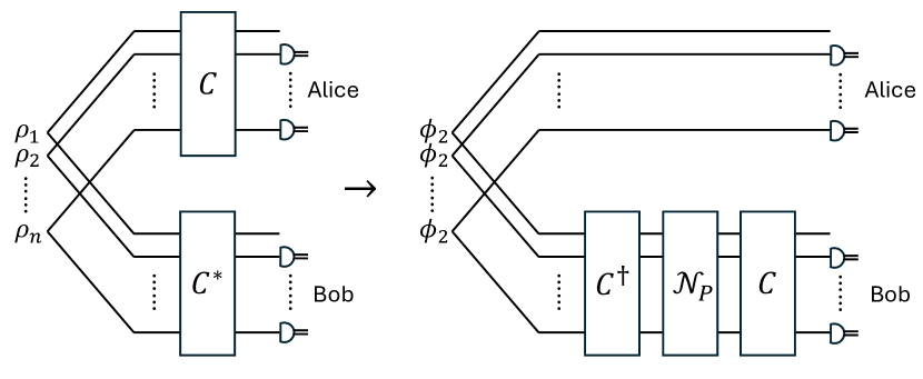
Figure 1: Circuit of an $n$-to-1 bilocal Clifford entanglement purification (biCEP) protocol using an $n$-qubit Clifford $C$. The input states are $n$ two-qubit states $\rho_{1},\dots,\rho_{n}$ which are distributed between two parties, Alice and Bob. On the right hand side of this figure we demonstrate the mechanism of biCEP circuit, i.e. transformation of Pauli errors.

We have demonstrated that an LOCC-implementable EPP which is universal for all entangled states cannot exist. Now we want to find protocols that are universal for restricted input states, especially those with sufficiently high fidelity. We turn to the $n$-to-1 bilocal Clifford entanglement purification (biCEP) protocols [42] (shown in Fig. 1), and study their universal properties. The $n$-to-1 biCEP protocols are defined as follows.

Definition 4 ($n$-to-1 biCEP [42]).

In an $n$-to-1 biCEP protocol, Alice applies $n$-qubit Clifford $C$ on her $n$ qubits while Bob performs the entry-wise complex conjugate of $C$, i.e. $C^{*}$, on his $n$ qubits. Then Alice and Bob measure in computational basis their last $(n-1)$ qubits and communicate the measurement outcomes. The protocol is considered successful if all $(n-1)$ pairs of measurement outcomes have the same parity (00 or 11), and unsuccessful otherwise.

The choice of biCEP has two motivations: (i) Clifford operations can be realized via finite layers of standard single- and two-qubit gates, e.g. the Hadamard gate, phase gate, CNOT gate and CZ gate [43, 44, 45, 46], which guarantees practicality; (ii) the $n$-to-1 biCEP family covers EPPs that can be constructed from all $[[n,1,d]]$ stabilizer codes [47, 37], which demonstrates the connection between EPP and quantum error correction. As the successful output of biCEP protocols only depends on the diagonal elements of input states’ density matrices in the Bell basis (see Sec. III.A.4 of the Supplemental Material [37]), we assume BDS input without loss of generality, which is also practically justified by Pauli twirling [48, 49, 50]. We further specify that we will focus on “complete BDS sets” as input sets, which are complete in the sense that they contain the objective noiseless Bell state and cover all three possible Pauli errors.

Definition 5 (Complete BDS set).

A set of BDS, $\mathcal{S}$, is a complete BDS set if (i) every $\rho\in\mathcal{S}$ is entangled, (ii) $\phi_{2}\in\mathcal{S}$, and (iii) $\exists\rho_{1},\rho_{2},\rho_{3}\in\mathcal{S}$ s.t. $|\psi^{+}\rangle\in\mathrm{supp}(\rho_{1}),|\psi^{-}\rangle\in\mathrm{supp}(\rho_{2}),|\phi^{-}\rangle\in\mathrm{supp}(\rho_{3})$, where $\mathrm{supp}(\cdot)$ denotes operator support. Let $\mathfrak{C}$ be the collection of all such sets.

We emphasize that we allow the lowest fidelity of a state in such sets to be arbitrarily close to 1. For example, a complete BDS set could be a family of high-fidelity isotropic states $\{\rho:\rho=F\phi_{2}+(1-F)\tfrac{I-\phi_{2}}{3},F>1-\epsilon\}$ for any $1/2>\epsilon>0$.

The mechanism of biCEP protocols can be understood as follows (see more details in Sec. III.A.3 of the Supplemental Material [37]). For $n$ BDS $\rho_{1},\cdots,\rho_{n}$, the total state $\bigotimes_{i=1}^{n}\rho_{i}$ equals the output of $\phi_{2}^{\otimes n}$ through a unilateral Pauli channel $I\otimes\mathcal{N}_{P}(\phi_{2}^{\otimes n})$, where $\mathcal{N}_{P}(\rho)=\sum_{i=1}^{4^{n}}p_{i}P^{(n)}_{i}\rho P^{(n)}_{i}$ with $P^{(n)}_{i}$ being an $n$-qubit Pauli string, and $p_{i}$ the corresponding probability of $P_{i}^{(n)}$. Then we can see that the effect of the biCEP circuit is equivalent to transforming the unilateral Pauli channel into $\tilde{\mathcal{N}}_{P}(\rho)=\sum_{i=1}^{4^{n}}p_{i}\tilde{P}^{(n)}_{i}\rho\tilde{P}^{(n)}_{i}$, where each $P_{i}^{(n)}$ is transformed to another $\tilde{P}^{(n)}_{i}=CP^{(n)}_{i}C^{\dagger}$ via the conjugate of Clifford $C$.

It is clear that the error detection of biCEP is based on the Pauli string transformation capability of its Clifford $C$, and the transformed Pauli noise channel determines success or failure. Therefore, we can identify every biCEP by a single Clifford operator $C$. Our present goal is to identify the necessary and sufficient condition for biCEP to be universal for $\mathcal{S}\in\mathfrak{C}$ as Lemma 7. We first define a class of Pauli strings that will simplify description.

Definition 6 (Harmless string).

An $n$-qubit harmless string $P_{h}^{(n)}$ satisfies one of the following two conditions: (i) its first (leftmost) component is the identity operator $I$ and the remaining $n-1$ components are either the identity operator $I$ or Pauli $Z$, e.g. $I\otimes I\otimes Z$, or (ii) there exist at least one Pauli $X$ or $Y$ operator among its $n-1$ components other than the first one, e.g. $Y\otimes I\otimes X$.

The definition is motivated as follows: If a type (i) harmless string is applied unilaterally to $\phi_{2}^{\otimes n}$, the $(n-1)$-pair computational basis measurement outcomes will have identical parities as those of $\phi_{2}^{\otimes n}$, indicating success, while the first slot is not affected by Pauli error resulting in a noiseless $\phi_{2}$; if type (ii) harmless string is applied then the resulting state will indicate a failure.

Lemma 7 (Universality condition for biCEP).

An $n$-to-1 biCEP protocol using $n$-qubit Clifford $C$ is universal $\forall\mathcal{S}\in\mathfrak{C}$ if and only if $C$ transforms all $n$-qubit Pauli strings which have at least one identity operator into harmless strings only.

The proof is in Sec. III.B of the Supplemental Material [37]. For necessity we consider a special case where at least one input is noiseless, and then according to the definition of universality the successful output fidelity must be one. Moreover, as we have not assumed any knowledge of input states, the $n$ input states have to be arbitrarily ordered, while the first slot is always unmeasured. Therefore, the unilateral noise Pauli channel could include all possible $n$-qubit Pauli strings which have at least one identity operator. If they are transformed to harmless strings, as long as the biCEP measurement outcomes indicate success, the unmeasured pair is guaranteed to be noiseless. The proof of sufficiency is based on a formal expression of successful biCEP outcome fidelity and some technical lower bounding.

Notice that the set of all entangled isotropic states is a complete BDS set, so Theorem 3 together with Lemma 7 implies the non-existence of an universal biCEP:

Proposition 8.

For any $\mathcal{S}\in\mathfrak{C}$ and $n\geq 2$, $n$-to-1 biCEP protocols cannot be universal for $\mathcal{S}$.

We also provide an algebraic proof of this Proposition, which can be found in Sec. III.C of the Supplemental Material [37].

No non-trivial universal biCEP with ordered fidelity— So far we have made minimal assumptions about the input states, which strengthens the requirement of universality. In principle, we can obtain information about the input states, especially the ordering of their fidelities. In practice, we know when an entangled pair is successfully generated based on the heralding signal, and it is generally safe to assume that the latest generated state has the highest fidelity. We can take advantage of such ordered fidelity to relax the universality requirement. Specifically, we may choose to always keep the qubits of the highest-fidelity input unmeasured, which gives the following relaxed necessary condition for a biCEP to be universal with ordered fidelity:

Lemma 9 (Necessary condition for universal biCEP with ordered fidelity).

Given ordered fidelity, if a biCEP protocol using $n$-qubit Clifford $C$ is universal for $\mathcal{S}\in\mathfrak{C}$, $C$ transforms all $n$-qubit Pauli strings in the form of $I\otimes P$, where $P$ is an arbitrary $(n-1)$-qubit Pauli string, into harmless strings only.

The proof is omitted due to its similarity to the proof of Lemma 7, with the only change being that we fix the leftmost component of the Pauli strings to be the identity operator $I$. Here we emphasize that there always exists a trivial universal biCEP for complete BDS set given ordered fidelity: We can simply discard $(n-1)$ input states except for the one with the highest fidelity, and then the “ successful output” will always have fidelity equal to the highest input fidelity. Given this relaxed necessary condition, finding a non-trivial universal biCEP might be possible, as we can sweep over Cliffords that satisfy this condition. However, we prove that these protocols are always trivial, i.e., the output fidelity is always equal to the highest input fidelity:

Proposition 10.

Given ordered fidelity, every universal biCEP protocol for complete BDS sets does not perform better than the trivial protocol.

The proof can be found in Sec. III.D of the Supplemental Material [37].

Entanglement-assisted biCEP—

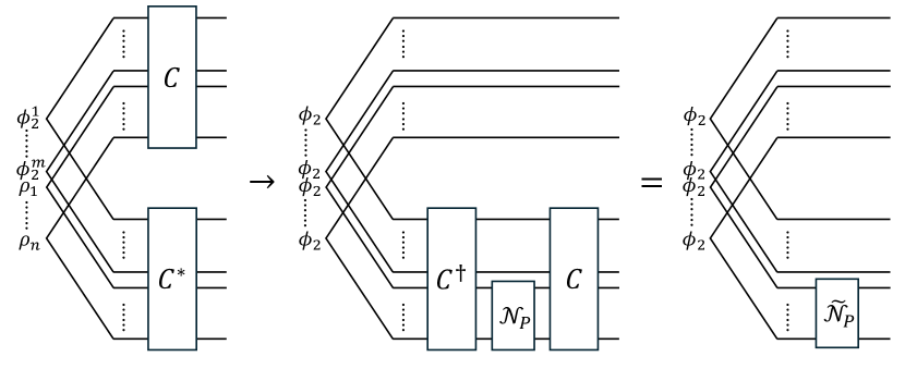
Figure 2: Visualization of $n$-to-1 biCEP assisted by $m$ noiseless Bell states $\phi_{2}$. Entanglement assistance requires that at the end of the circuits the assisting Bell states are unchanged. Final measurements are omitted in this figure.

We can further generalize our study of biCEP protocols to the scenario where we are supplied with $m$ pure Bell states, which can be input to the entanglement purification circuit, but must remain unchanged at the end. Assuming the unilateral Pauli channel corresponding to the total state of certain $n$ BDS is $\mathcal{N}_{P}$, the total state of $m$ pure Bell states together with the $n$ BDS corresponds to another unilateral Pauli channel $\mathcal{N}_{P}^{\prime}$ where the Kraus operators of $\mathcal{N}_{P}^{\prime}$ are simply the Kraus operators of $\mathcal{N}_{P}$ tensored with $m$ identity operators. The scenario of entanglement-assisted biCEP is visualized in Fig. 2. Note that multiplication relations and commutators between Pauli strings are unchanged if all relevant Pauli strings are tensored with with an equal number of identity operators. Therefore, the algebraic proofs of Proposition 8 and Proposition 10 still apply to these scenarios with pure Bell state assistance for biCEP. Combining all the above results on biCEP, we have the following theorem.

Theorem 11 (No universal biCEP).

There is no $n$-to-1 biCEP that is universal or non-trivially universal with ordered fidelity, when assisted by $m$ pure Bell states, $\forall\mathcal{S}\in\mathfrak{C}$, $\forall n\geq 2$, $\forall m>0$.

Discussion— In summary, we have introduced a property of EPPs that is desirable in practice, universality; we found a unique PPT-preserving protocol that is universal for all entangled states with fidelity greater than 1/2, and we proved that it is not a separable operation, thus not LOCC-implementable. Subsequently, we relaxed the requirement by restricting ourselves to states with arbitrarily high fidelity, but it turned out that universal protocols are still practically challenging since they cannot be realized by bilocal Clifford circuits. Moreover, we showed that if fidelity ordering of input states is provided, any biCEP that is universal is necessarily trivial, meaning that the purification output always has the same fidelity as the state with the highest fidelity. The results for biCEP hold even if assisted by an arbitrary number of pure Bell states.

In the context of distributed quantum information processing, our results imply that 1G quantum repeaters [51, 52] which distribute high-fidelity entanglement over long distance are difficult to construct without using large amount of physical resources and taking advantage of additional information such as underlying error patterns (see more detailed discussion in Sec. I of the Supplemental Material [37]). Universality of the DEJMPS protocol for rank-3 BDS implies that biased (Pauli) noise is favorable; such biased noise can be obtained in various physical platforms, e.g. neutral atoms [53], and stabilized cat qubits encoded in bosonic systems [55, 56, 57]. From a theoretical perspective, our work advanced the beyond-i.i.d. literature, by contributing to the fundamental understanding of entanglement purification with non-i.i.d. input [58, 59, 60]. We derived new fundamental limits on the capability of LOCC and provided a new example of operational gap between PPT and SEP (LOCC) in low dimensions. We also deepened the understanding of Clifford gates by revealing interesting structures of $n$-qubit Pauli group under Clifford conjugate.

Our introduction of universality opens up various new research directions. For example, it would be interesting to go beyond EPPs for two-qubit states and study universality of qudit EPPs, and multi-partite EPPs, e.g. for graph states [61, 62, 63, 64, 65, 9]. The idea of universality can also be extended to magic state distillation [66, 67] where magic states will become non-identical if they undergo different number of distillation cycles. Furthermore, the presented no-go results have not ruled out all possibilities of LOCC-implementable EPPs that are universal for two-qubit states with arbitrary error patterns, because we could in principle further increase the allowed lowest fidelity of input states and consider other EPPs beyond biCEP. There should then exist a larger parameter space of PPT universal entanglement purification protocols, and it is possible that some of these PPT entanglement purification protocols are LOCC-implementable. The search for separable universal entanglement purification protocol with higher fidelity threshold is an important next step that may require discovery of new techniques to determine separability for quantum states with symmetry [68, 69].

Acknowledgments— We acknowledge support from the NSF Quantum Leap Challenge Institute for Hybrid Quantum Architectures and Networks (NSF Award 2016136). T.Z. would like to acknowledge the support from the Marshall and Arlene Bennett Family Research Program. X.C. and E.C. are supported by the U.S. Department of Energy Office of Science National Quantum Information Science Research Centers.

Supplemental Material

I Motivation for introducing universality

Analysis of entanglement purification protocols (EPPs) connects beyond-i.i.d. quantum information theory, entanglement theory, and other advanced mathematical structures. As a property of both the purification protocol and the input state set, universality is an interesting theoretical topic on its own. Here we elaborate on the motivation for introducing universality with special attention to practical considerations. Although we consider entanglement distribution quantum networks as the main application of this work, our discussion also applies to general quantum information processing architectures which use imperfect quantum memories to store quantum states and run probabilistic operations, with purification/distillation protocols as examples.

I.1 Requirements for benchmarking, optimization and scheduling in quantum networks

Once built, quantum networks [23, 24] will serve as the infrastructure necessary for distributed quantum information processing (QIP). Quantum networks will be used to distribute entanglement that will be in turn consumed by network applications. Most currently envisioned quantum applications consume specific forms of entangled states. For example, quantum state teleportation [25] and gate teleportation [70], operations required for distributed quantum computing [19, 20], both consume EPR pairs, and quantum sensing [22] with beyond standard quantum limit performance consumes multi-partite entangled states such as spin-squeezed states or GHZ states.

Distributing entanglement over long-distances will require long duration of operations, leading to significant idling decoherence. This poses strict requirements on counteracting its effects. Counteracting decoherence can be achieved by (i) quantum error correction (QEC) [1, 2, 3, 4, 5] which protects encoded quantum information by continuous monitoring and active correction, and (ii) quantum error detection, with various examples of quantum state purification/distillation protocols [6, 7, 8, 9, 10]. Due to the requirement of active correction, QEC is more challenging in practice. Therefore, we do not anticipate that QEC can be practically incorporated in near-term QIP architectures, especially quantum networks, and this justifies our focus on entanglement purification protocols in this work.

In entanglement distribution quantum networks, the probabilistic nature of operations leads to the non-identicality of entangled states. Long distance communication requires using photons as flying qubits to mediate remote entanglement generation. Errors occur due to losses during photon transmission and the fundamental limit on success probability of linear optical Bell state measurements [71], which do not seem solvable in the near future. Probabilistic entanglement generation requires storing successfully generated entangled states in quantum memories with two uses: (i) quantum networks resort to divide-and-conquer strategy to avoid exponentially decaying communication success probability with distance [72]; (ii) entanglement purification needs multiple entangled states as inputs. As a result, the earlier generated states stored in quantum memories accumulate errors due to idling decoherence, leading to non-identicality of the entangled states. The non-identicality is exacerbated by the states spending different amounts of idling time in quantum memories. The non-identicality occurs even if the originally generated states were identical. In addition, entanglement purification is also probabilistic. Therefore, entangled states could have undergone different levels of purification, which naturally could be non-identical.

It has been shown that EPPs can be optimized if the input states are known [73, 74], and the optimal solution may depend on the input states and the operation error models. However, knowledge of the input states is non-trivial. The states are determined by their form during successful entanglement generation, and the idling error accumulated between the successful state generation and the start of entanglement purification. As a result, to determine the form of the input states, we need to know both the initial state and the idling error model. Although information about the quantum states and channels can be learned through measurements, we cannot directly measure the states prior to EPP, as this would corrupt them. Therefore, the information must be obtained earlier, either through state and process tomography, or through specialized quantum benchmarking/learning protocols [28, 29, 30, 31]. However, there is no guarantee that the information about the initial states and the error processes will coincide with the current input states. In other words, even if we can learn information about the errors, we can only obtain optimal solution for the specific problem corresponding to a scenario in the past, while error processes vary over time [32, 33]. We could argue that we do not need an accurate knowledge of the quantum states to obtain close-to-optimal protocols. Such solutions could be an interesting subject of future work, but but finding them may be difficult because the transition between optimal solutions can be abruptly different when error processes change [75]. Even if the quantum processes are stationary, additional resources such as repeated measurements are required in order to learn the details from the processes.

Coordinating the actions of the large number of components in quantum networks requires scheduling optimization, including optimization of entanglement swapping and purification. Scheduling policy optimization is difficult due to the large state space, and optimal policy is only known for the simplest scenarios that do not include entanglement purification [76]. For instance, in quantum repeater networks with entanglement generation buffer time [77, 78] or continuous (pre-) entanglement generation [79, 80, 81, 82], additional idling time is intentionally introduced to optimize entanglement distribution rate and latency, and entanglement purification can be performed within the time windows before entanglement is requested. This enlarges the parameter space for optimization. We consider the scenario where we schedule a fixed EPP. Although there is no known EPP that is universal for arbitrary Bell diagonal states with a certain fidelity threshold, it is still possible that existing EPPs can offer positive fidelity gain with non-identical input states conditioned on success, but the requirement on small difference between input states could be stringent. For example, we consider the well-known 2-to-1 DEJMPS protocol [7] and isotropic states as inputs. If one input has fidelity 0.9 and the other input has fidelity 0.85, the successful output fidelity will be $F^{\prime}(0.9,0.85)\approx 0.9055>0.9$; meanwhile, if we fix the 0.9 fidelity input and change the other input to have 0.83 fidelity, the successful output fidelity will be $F^{\prime}(0.9,0.83)\approx 0.8967<0.9$. Note that when the input fidelities increase, the difference will be even smaller. Therefore, in order to ensure non-trivial fidelity increase, we must wisely choose from all available entangled pairs. To decide, we must calculate the output fidelities for every possible combination of input states, which introduces additional computational overhead, and requires the knowledge of entangled states.

In summary, there are two approaches to distributing high-fidelity entanglement with entanglement purification: (i) optimizing EPPs, and (ii) optimizing the scheduling for fixed EPPs. However, both approaches have a significant optimization overhead, and also require knowledge of quantum states which results in a quantum benchmarking overhead.

I.2 Relaxed requirements for universal entanglement purification protocols

In the above, we discussed the operational requirements in quantum networks from an engineering and an architectural perspective. It is clear that when the adopted EPP is not universal for arbitrary error models, the required operational overhead is very costly. In contrast, a universal EPP is a “one-cure-for-all” solution, and the requirements can be relaxed, as explained in the following.

First, assume there exists a universal EPP for arbitrary error models. There is no need to know the underlying error models of quantum memories and entanglement generation. It suffices to know that the input states have a fidelity above the fidelity threshold of the universal EPP. This can be done e.g. by lower bounding the fidelity based on results of rough quantum benchmarking, which significantly reduces the resource overhead.

Second, although a fixed universal EPP is not necessarily the optimal protocol for some specific input states, it is guaranteed that the successful output will always be non-trivial, i.e. the successful output fidelity will always at least as high as the highest input fidelity. This is operationally desirable, and therefore unless a better performance is required, using a universal EPP can avoid the need to perform additional purification circuit optimizations.

Finally, a universal EPP strongly relaxes the scheduling requirements. A universal EPP only requires that every input state has a fidelity above the fidelity threshold, which can be verified individually, and cross-referencing other entangled pairs’ information is not needed. For instance, we can employ a memory-wise cut-off policy. Approximate information about initial state and error models allows lower bounding entanglement fidelity. We only need to re-initialize the quantum memories at a certain cut-off time when we can no longer guarantee that the fidelity is above the threshold. The states can be used for EPP at any time before the cut-off.

II General entanglement purification protocols

In this section, we offer elaborated discussion on general entanglement purification protocols, i.e. we simply view EPPs as two-branch quantum instruments while ignoring their explicit implementation. In Sec. II.1, we briefly review the needed background information on state-operation duality and the conditions for quantum operation to be PPT and SEP, respectively. We also present a self-contained overview of a computable separability criterion, i.e. the Bloch representation criterion, which proves to be useful for studying separability of Choi states which are of our interest. Then in Sec. II.2 we prove technical results which allow us to include the boundary of entangled state set when studying universality. Subsequently, we prove the unique form of Choi state for PPT entanglement purification protocols that are universal for all entangled states with fidelity above 1/2 (Proposition 2 in the main text) in Sec. II.3. Finally in Sec. II.4, based on the Bloch representation criterion and the explicit form of Choi state, we prove that the Choi states are non-SEP for arbitrary even $n\geq 2$, and moreover, the Choi states for odd $n>2$ are also non-SEP. We also include a brief, interesting spin-off discussion on the elementary function representation of a special case of hypergeometric function, which is closely related to the combinatorial proof of non-separability of the Choi states for even $n\geq 2$.

II.1 Preliminaries

Recall that we define general EPP as a two-branch quantum instrument $\mathcal{E}=\{\mathcal{E}_{0},\mathcal{E}_{1}\}$, where CPTNI maps $\mathcal{E}_{0}$ and $\mathcal{E}_{1}$ correspond to success and failure, respectively.

II.1.1 State-operation duality

The effect of the operation $\mathcal{E}_{0}$ (the successful branch of $n$-to-1 EPP $\mathcal{E}$) can be described by the Choi operator (matrix, state) $J=(\mathrm{Id}^{A_{1}B_{1}\cdots A_{n}B_{n}}\otimes\mathcal{E}_{0}^{A_{1}^{\prime}B_{1}^{\prime}\cdots A_{n}^{\prime}B_{n}^{\prime}})(|\Omega\rangle\langle\Omega|)$, where $|\Omega\rangle=\sum_{i}|i\rangle_{A_{1}B_{1}\cdots A_{n}B_{n}}|i\rangle_{A_{1}^{\prime}B_{1}^{\prime}\cdots A_{n}^{\prime}B_{n}^{\prime}}$ and $|i\rangle_{A_{1}B_{1}\cdots A_{n}B_{n}}$ are basis vectors of the $2n$-qubit (EPP input) Hilbert space. As an instance of state-operation duality (isomorphism), the PPT and SEP properties of quantum operations are equivalent to the respective properties of their Choi state:

Lemma 12 (PPT operation).

A quantum operation $\mathcal{E}:\mathcal{L}(\mathcal{H}_{A}\otimes\mathcal{H}_{B})\rightarrow\mathcal{L}(\mathcal{H}_{\hat{A}}\otimes\mathcal{H}_{\hat{B}})$ is PPT if and only if its Choi matrix $J\in\mathcal{L}(\mathcal{H}_{A}\otimes\mathcal{H}_{B}\otimes\mathcal{H}_{\hat{A}}\otimes\mathcal{H}_{\hat{B}})$ is PPT with respect to the $A\hat{A}$-$B\hat{B}$ partition.

Lemma 13 (SEP operation).

A quantum operation $\mathcal{E}:\mathcal{L}(\mathcal{H}_{A}\otimes\mathcal{H}_{B})\rightarrow\mathcal{L}(\mathcal{H}_{\hat{A}}\otimes\mathcal{H}_{\hat{B}})$ is separable if and only if its Choi matrix $J\in\mathcal{L}(\mathcal{H}_{A}\otimes\mathcal{H}_{B}\otimes\mathcal{H}_{\hat{A}}\otimes\mathcal{H}_{\hat{B}})$ is separable with respect to $A\hat{A}$-$B\hat{B}$ partition.

An EPP $\mathcal{E}=\{\mathcal{E}_{0},\mathcal{E}_{1}\}$ is in SEP if both the success and the failure branches are SEP operations, i.e. if the Choi operators of $\mathcal{E}_{0}$ and $\mathcal{E}_{1}$ are both separable [35, 83], while it is in PPT if both branches are PPT operations, i.e. if both Choi operators have a positive partial transpose [36, 84, 85]. Note that whenever the Choi operator of $\mathcal{E}_{0}$ is separable, we can always replace the unwanted state $\mathcal{E}_{1}(\rho)/\mathrm{tr}(\mathcal{E}_{1}(\rho))$ with the maximally mixed state, making the EPP separable. The same argument applies if the Choi operator of $\mathcal{E}_{0}$ is PPT.

II.1.2 Bloch representation separability criteria

As mentioned in the main text, for bipartite states on the $M\times N$-dimensional Hilbert space (one party has dimension $M$ and the other $N$), they have the following general Bloch decomposition

$$\rho=\frac{1}{MN}\left(I_{M}\otimes I_{N}+\sum_{i=1}^{M^{2}-1}r_{i}\lambda_{i}\otimes I_{N}+\sum_{j=1}^{N^{2}-1}s_{j}I_{M}\otimes\tilde{\lambda}_{j}+\sum_{i=1}^{M^{2}-1}\sum_{j=1}^{N^{2}-1}t_{ij}\lambda_{i}\otimes\tilde{\lambda}_{j}\right)$$ (1)

where $\lambda_{i}$ are $\mathrm{SU}(M)$ generators and $\tilde{\lambda}_{j}$ are $\mathrm{SU}(N)$ generators. Based on this representation, we have the following necessary and sufficient condition for bipartite separable states, and a derived necessary condition for bipartite separability [41] which is used in this work. We provide simple proofs for both.

Lemma 14 (Necessary and sufficient condition of separability [41]).

A bipartite state $\rho_{AB}$ on $\mathcal{H}_{A}\otimes\mathcal{H}_{B}$ is separable if and only if there exist triples $(0\leq p_{i}\leq 1,\mathbf{u}_{i},\mathbf{v}_{i})$, $\sum_{i}p_{i}=1$ such that its Bloch representation satisfies $T=\sum_{i}p_{i}\mathbf{u}_{i}\mathbf{v}_{i}^{T}$, $\mathbf{r}=\sum_{i}p_{i}\mathbf{u}_{i}$, $\mathbf{s}=\sum_{i}p_{i}\mathbf{v}_{i}$.

Proof.

First we note that a bipartite state $\rho_{AB}$ is a pure separable state $\rho=|\psi\rangle\langle\psi|_{A}\otimes|\varphi\rangle\langle\varphi|_{B}$ if and only if its Bloch representation (Eqn. 1) satisfies $T=\mathbf{r}\mathbf{s}^{T}$ with $\lVert\mathbf{r}\rVert_{2}=\sqrt{M(M-1)/2}$ and $\lVert\mathbf{s}\rVert_{2}=\sqrt{N(N-1)/2}$, where $\mathbf{r},\mathbf{s}$ are the column vectors with each component being $r_{i},s_{j}$, respectively. The matrix equation guarantees that $\rho=\rho_{A}\otimes\rho_{B}$ where $\rho_{A(B)}=\mathrm{Tr}_{B(A)}(\rho)$, and the 2-norm (Euclidean norm) condition guarantees that $\rho_{A(B)}$ are pure.

Now observe that any bipartite state $\rho_{AB}$ is separable if and only if it can be decomposed into a weighted sum of pure separable states. We complete the proof using the above condition for a pure separable state. ∎

Corollary 14.1 (Necessary condition of separability [41]).

If a bipartite state $\rho_{AB}$ on $\mathcal{H}_{A}\otimes\mathcal{H}_{B}$ is separable, then its coefficient matrix $T_{ij}=t_{ij}$ must satisfy

$$\lVert T\rVert_{1}=\mathrm{Tr}(\sqrt{T^{\dagger}T})\leq\frac{\sqrt{MN(M-1)(N-1)}}{2},$$

where $M=\dim\mathcal{H}_{A},N=\dim\mathcal{H}_{B}$, and $\lVert\cdot\rVert_{1}$ denotes 1-norm which equals the sum of the singular values, i.e. $\lVert T\rVert_{1}=\mathrm{Tr}(\sqrt{T^{\dagger}T})$.

Proof.

According to the inequality of singular values (triangle inequality of 1-norm), i.e. $\lVert A+B\rVert_{1}\leq\lVert A\rVert_{1}+\lVert B\rVert_{1}$, we have that for the $T$ matrix of a separable bipartite state

$$\lVert T\rVert_{1}= \lVert\sum_{i}p_{i}\mathbf{u}_{i}\mathbf{v}_{i}^{T}\rVert_{1}\leq\sum_{i}p_{i}\lVert\mathbf{u}_{i}\mathbf{v}_{i}^{T}\rVert_{1}$$ (2)

$$= \frac{\sqrt{MN(M-1)(N-1)}}{2}\sum_{i}p_{i}\lVert\mathbf{e}_{\mathbf{u}_{i}}\mathbf{e}_{\mathbf{v}_{i}}^{T}\rVert_{1}=\frac{\sqrt{MN(M-1)(N-1)}}{2}$$

where $\mathbf{e}_{\mathbf{u}_{i}(\mathbf{v}_{i})}$ is the unit vector in the same direction as $\mathbf{u}_{i}(\mathbf{v}_{i})$, and for the last equality we use the fact that for the outer product of two unit vectors, in singular value decomposition we can always find unitaries $U,V$ (in this specific case we may only need real orthogonal matrices as $\mathbf{u}_{i},\mathbf{v}_{i}$ are real) such that $U\mathbf{e}_{\mathbf{u}_{i}}\mathbf{e}_{\mathbf{v}_{i}}^{T}V^{\dagger}=\mathrm{diag}(1,0,0,\dots,0)$, and thus the sum of the singular values is guaranteed to be 1. ∎

II.2 Continuity of completely positive maps and boundaries of entangled states

II.2.1 Results on trace distance

It is well known that the trace distance $d(X,Y)=\frac{1}{2}\|X-Y\|_{1}$ is monotonic under completely positive and trace-preserving maps [86]. Here we establish monotonicity under general completely positive trace-non-increasing (CPTNI) maps with a similar proof:

Theorem 15.

For any completely positive and trace-non-increasing map $\mathcal{E}$, we have $d(\mathcal{E}(\rho),\mathcal{E}(\sigma))\leq d(\rho,\sigma)$.

Proof.

First we prove that for two positive operators $X$ and $Y$ that are not necessarily unit trace, there exists an operator $0\leq P\leq\mathbb{I}$ such that

$$d(X,Y)=\mathrm{tr}(P(X-Y)).$$ (3)

To show this, let us write the spectral decomposition of $X-Y$ as $A-B$, where $A$ and $B$ are both positive operators and have orthogonal support. Then, $d(X,Y)=\frac{1}{2}\mathrm{tr}|X-Y|=\frac{1}{2}\mathrm{tr}|A-B|=\frac{1}{2}(\mathrm{tr}A+\mathrm{tr}B)$. Suppose without loss of generality $\mathrm{tr}A\geq\mathrm{tr}B$. Let $P^{\prime}$ be the projector onto the support of $A$ and define $P=\frac{\mathrm{tr}A+\mathrm{tr}B}{2\mathrm{tr}A}P^{\prime}$. Then,

$$\mathrm{tr}(P(X-Y))=\mathrm{tr}(P(A-B))=\frac{\mathrm{tr}A+\mathrm{tr}B}{2\mathrm{tr}A}\mathrm{tr}(P^{\prime}(A-B)P^{\prime})=\frac{1}{2}(\mathrm{tr}A+\mathrm{tr}B)=d(X,Y).$$ (4)

Now we apply this result to $\mathcal{E}(\rho)$ and $\mathcal{E}(\sigma)$. Let $0\leq Q\leq\mathbb{I}$ be an operator such that $d(\mathcal{E}(\rho),\mathcal{E}(\sigma))=\mathrm{tr}(Q\mathcal{E}(\rho)-Q\mathcal{E}(\sigma))$. Suppose $\rho-\sigma$ has the spectral decomposition $C-D$ where $C$ and $D$ are both positive operators and have orthogonal support. Since $\mathrm{tr}\rho-\mathrm{tr}\sigma=0$, we have $\mathrm{tr}C=\mathrm{tr}D$. Now,

$$d(\rho,\sigma) =\frac{1}{2}\mathrm{tr}|\rho-\sigma|=\frac{1}{2}\mathrm{tr}|C-D|=\frac{1}{2}(\mathrm{tr}C+\mathrm{tr}D)=\mathrm{tr}C\geq\mathrm{tr}\mathcal{E}(C)\geq\mathrm{tr}(Q\mathcal{E}(C))\geq\mathrm{tr}(Q\mathcal{E}(C)-Q\mathcal{E}(D))$$

$$=\mathrm{tr}(Q\mathcal{E}(\rho)-Q\mathcal{E}(\sigma))=d(\mathcal{E}(\rho),\mathcal{E}(\sigma)),$$ (5)

where the first inequality follows from the fact that $\mathcal{E}$ is trace-non-increasing, the second inequality follows from $Q\leq\mathbb{I}$, and the third inequality follows from the positivity of $Q$ and $\mathcal{E}(D)$. ∎

Lemma 16.

$d\left(\bigotimes_{i}\rho_{i},\bigotimes_{i}\sigma_{i}\right)\leq\sqrt{2\sum_{i}d(\rho_{i},\sigma_{i})}$.

Proof.

The proof starts with the Fuchs–van de Graaf inequality, and follows with a straightforward derivation:

$$d\left(\bigotimes_{i}\rho_{i},\bigotimes_{i}\sigma_{i}\right) \leq\sqrt{1-F\left(\bigotimes_{i}\rho_{i},\bigotimes_{i}\sigma_{i}\right)}$$ (6)

$$=\sqrt{1-\prod_{i}F(\rho_{i},\sigma_{i})}$$ (7)

$$\leq\sqrt{1-\prod_{i}\left[1-d\left(\rho_{i},\sigma_{i}\right)\right]^{2}}$$ (8)

$$\leq\sqrt{1-\left(1-2\sum_{i}d(\rho_{i},\sigma_{i})\right)}$$ (9)

$$=\sqrt{2\sum_{i}d(\rho_{i},\sigma_{i})},$$ (10)

where the first equality follows from the fact that fidelity is multiplicative under tensor products; the second inequality is from another application of Fuchs–van de Graaf inequality; the third inequality is obvious by recalling $0\leq d(\rho_{i},\sigma_{i})\leq 1$. ∎

II.2.2 The boundary of an input state set

Using the above results, it is easy to prove the following statement:

Theorem 17.

A purification protocol is universal for a set of states $S$ if and only if it is universal for $S\cup\partial S$, where $\partial S$ is the boundary of $S$.

Proof.

The if direction is clear. To show the converse, suppose a purification protocol $\mathcal{E}=(\mathcal{E}_{0},\mathcal{E}_{1})$ is not universal for $S\cup\partial S$. This means that there exist states $\rho_{1},\cdots,\rho_{n}\in S\cup\partial S$ such that

$$F\left(\frac{\mathcal{E}_{0}(\rho)}{\mathrm{tr}\mathcal{E}_{0}(\rho)}\right)<\max_{i}F(\rho_{i}),$$ (11)

where $\rho=\bigotimes_{i=1}^{n}\rho_{i}$, and we have omitted the reference state which is the maximally entangled state. If all of $\rho_{i}\in S$, then this means $\mathcal{E}$ cannot be universal for $S$. Therefore, we focus on the case where at least one of $\rho_{i}\in\partial S\setminus S$. According to the definition of the boundary, for any point $x\in\partial S$, there exists in every neighborhood of $x$ a point that is in $S$. If we replace each such $\rho_{i}$ by a state $\tilde{\rho_{i}}\in S$ that is $\epsilon$ close to $\rho_{i}$ in trace distance and define $\tilde{\rho}=\left(\bigotimes_{\rho_{i}\in\partial S\setminus S}\tilde{\rho_{i}}\right)\otimes\left(\bigotimes_{\rho_{j}\in S}\rho_{j}\right)$, we deduce

$$d(\tilde{\rho},\rho)\leq\sqrt{2n\epsilon}.$$ (12)

Thus by monotonicity of trace distance under CPTNI map, we get

$$d(\mathcal{E}_{0}(\tilde{\rho}),\mathcal{E}_{0}(\rho))\leq\sqrt{2n\epsilon}.$$ (13)

By continuity of trace distance and fidelity, this means that $\left|F\left(\frac{\mathcal{E}_{0}(\tilde{\rho})}{\mathrm{tr}\mathcal{E}_{0}(\tilde{\rho})}\right)-F\left(\frac{\mathcal{E}_{0}(\rho)}{\mathrm{tr}\mathcal{E}_{0}(\rho)}\right)\right|$ can be made arbitrarily small by choosing arbitrarily small $\epsilon$. Therefore, we can always find $\tilde{\rho}$ as a tensor product of a state from set $S$ which violates the universality condition:

$$F\left(\frac{\mathcal{E}_{0}(\tilde{\rho})}{\mathrm{tr}\mathcal{E}_{0}(\tilde{\rho})}\right)<\max_{i}F(\rho_{i}),$$ (14)

which means that the protocol cannot be universal for $S$. ∎

Based on this result, we can safely include $F=1/2$ isotropic state in the set in the following when we consider possibility of universality for all qubit entangled isotropic states.

II.3 Choi matrix of $n$-to-1 universal EPP with fidelity threshold 1/2

Here we prove the Proposition 2 in the main text, while we rephrase the statement a bit by explicitly demonstrating the Choi operators.

Theorem 18.

There exist PPT $n$-to-$1$ entanglement purification protocols that are universal for all two-qubit states with fidelity greater than 1/2, given by the Choi operator $J_{n}=\left(\bigotimes_{i=1}^{n}\phi_{2}^{A_{i}B_{i}}\right)\otimes\phi_{2}^{\hat{A}\hat{B}}+\left(\bigotimes_{i=1}^{n}\left(\phi_{2}^{\perp}\right)^{A_{i}B_{i}}\right)\otimes\left(\phi_{2}^{\perp}\right)^{\hat{A}\hat{B}}/3$, where $\phi_{2}^{\perp}=I-\phi_{2}$. The protocols are unique up to twirling the input and output systems and a multiplicative constant $C\in(0,1]$ on the Choi operator which determines the probability of success.

Proof.

Let us first show that this entanglement purification protocol is PPT and universal. It is obvious that given the input states as $n$ isotropic states with fidelities $F_{1},F_{2},\dots,F_{n}$ the output fidelity of this operation is

$$F^{\prime}(F_{1},F_{2},\dots,F_{n})=\frac{\prod_{i=1}^{n}F_{i}}{\prod_{i=1}^{n}F_{i}+\prod_{i=1}^{n}(1-F_{i})}.$$ (15)

Now consider the difference $F^{\prime}(F_{1},F_{2},\dots,F_{n})-F_{j}$ as follows

$$F^{\prime}(F_{1},F_{2},\dots,F_{n})-F_{j}= \left(\frac{\prod_{i\neq j}F_{i}}{\prod_{i=1}^{n}F_{i}+\prod_{i=1}^{n}(1-F_{i})}-1\right)F_{j}$$ (16)

$$= \frac{\prod_{i\neq j}F_{i}-\prod_{i=1}^{n}F_{i}-\prod_{i=1}^{n}(1-F_{i})}{\prod_{i=1}^{n}F_{i}+\prod_{i=1}^{n}(1-F_{i})}F_{j}$$

$$= \frac{(1-F_{j})\left(\prod_{i\neq j}F_{i}-\prod_{i\neq j}(1-F_{i})\right)}{\prod_{i=1}^{n}F_{i}+\prod_{i=1}^{n}(1-F_{i})}F_{j}\geq 0,$$

for $F_{1},F_{2},\dots,F_{n}\geq 1/2$. This shows that the operation is universal for $n$ isotropic states with fidelity above 1/2, thus also universal for arbitrary $n$ states with fidelity above 1/2. The partial transpose of $J_{n}$ w.r.t. $A-B$ bipartition is

$$J_{n}^{T_{B}}=\frac{1}{2^{n+1}}\left[(P_{s}-P_{a})^{\otimes(n+1)}+\frac{1}{3}(P_{s}+3P_{a})^{\otimes(n+1)}\right],$$ (17)

since $\phi_{2}^{T_{B}}=\mathbb{F}/2=(P_{s}-P_{a})/2$ and $\left(\phi_{2}^{\perp}\right)^{T_{B}}=I-\mathbb{F}/2=(P_{s}+3P_{a})/2$, where $P_{s}$ and $P_{a}$ are projectors onto a 2-qubit symmetric subspace and an antisymmetric subspace, respectively. We observe all projectors’ coefficients from the second term are positive, while only the projectors that contain odd number of $P_{a}$ have negative coefficients from the first term, but their corresponding coefficients from the second term are guaranteed to have larger absolute value due to $3^{\#P_{a}}/3\geq 1$ for odd $\#P_{a}$, where $\#P_{a}$ denotes the number of $\#P_{a}$ in a tensor product of $(n+1)$ projectors. Therefore, the sum of the two terms gives a convex combination of projectors, which is positive, and thus $J_{n}$ is PPT.

For uniqueness, note that universal entanglement purification protocols necessarily output $\phi_{2}$ whenever one of the input states is $\phi_{2}$. Therefore, the Choi operator of any universal entanglement purification protocol must have the form (up to twirling)

$$J=\sum_{\vec{s}\in\{0,1\}^{\times n}}a_{\vec{s}}\left\{\bigotimes_{i=1}^{n}\left[\phi_{2}^{s_{i}}\left(\phi_{2}^{\perp}\right)^{1-s_{i}}\right]^{A_{i}B_{i}}\right\}\otimes\phi_{2}^{\hat{A}\hat{B}}+a\left[\bigotimes_{i=1}^{n}\left(\phi_{2}^{\perp}\right)^{A_{i}B_{i}}\right]\otimes\left(\phi_{2}^{\perp}\right)^{\hat{A}\hat{B}}/3$$ (18)

where $a\geq 0$ and $a_{\vec{s}}\geq 0\ \forall\,\vec{s}$. Now we have that

$$J^{T_{B}}\propto \sum_{\vec{s}\in\{0,1\}^{\times n}}a_{\vec{s}}\left\{\bigotimes_{i=1}^{n}\left[(P_{s}-P_{a})^{s_{i}}\left(P_{s}+3P_{a}\right)^{1-s_{i}}\right]^{A_{i}B_{i}}\right\}\otimes(P_{s}-P_{a})^{\hat{A}\hat{B}}$$ (19)

$$\quad+a\left[\bigotimes_{i=1}^{n}\left(P_{s}+3P_{a}\right)^{A_{i}B_{i}}\right]\otimes\left(P_{s}+3P_{a}\right)^{\hat{A}\hat{B}}/3$$ (20)

$J^{T_{B}}\geq 0$ implies in particular that the coefficient in front of $P_{s}^{\otimes n}\otimes P_{a}$ is non-negative. This means that

$$a\geq\sum_{\vec{s}}a_{\vec{s}}.$$ (21)

Now the fidelity of the output state conditioned on success is given by

$$F(F_{1},\cdots,F_{n})=\frac{\sum_{\vec{s}}a_{\vec{s}}\prod_{i=1}^{n}F_{i}^{s_{i}}(1-F_{i})^{1-s_{i}}}{\sum_{\vec{s}}a_{\vec{s}}\prod_{i=1}^{n}F_{i}^{s_{i}}(1-F_{i})^{1-s_{i}}+a\prod_{i=1}^{n}(1-F_{i})}.$$ (22)

In particular, when $F_{2}=F_{3}=\cdots=F_{n}=1/2$, we have

$$F(F_{1},1/2,\cdots,1/2)=\frac{\sum_{\vec{s}:s_{1}=1}a_{\vec{s}}F_{1}+\sum_{\vec{s}^{\prime}:s^{\prime}_{1}=0}a_{\vec{s}^{\prime}}(1-F_{1})}{\sum_{\vec{s}:s_{1}=1}a_{\vec{s}}F_{1}+\sum_{\vec{s}^{\prime}:s^{\prime}_{1}=0}a_{\vec{s}^{\prime}}(1-F_{1})+a(1-F_{1})}.$$ (23)

If $F_{1}\in(1/2,1)$ and at least one of $\{a_{\vec{s}}:s_{1}=0\}$ is positive, we have the strict inequality

$$F(F_{1},1/2,\cdots,1/2) <\frac{\sum_{\vec{s}:s_{1}=1}a_{\vec{s}}F_{1}+\sum_{\vec{s}^{\prime}:s^{\prime}_{1}=0}a_{\vec{s}^{\prime}}F_{1}}{\sum_{\vec{s}:s_{1}=1}a_{\vec{s}}F_{1}+\sum_{\vec{s}^{\prime}:s^{\prime}_{1}=0}a_{\vec{s}^{\prime}}F_{1}+a(1-F_{1})}\leq\frac{aF_{1}}{aF_{1}+a(1-F_{1})}=F_{1}.$$ (24)

Thus for the operation to be universal, it must be that $a_{\vec{s}}=0$ whenever $s_{1}=0$. By the same logic, we find that $a_{\vec{s}}$ must vanish whenever any $s_{i}=0$. Moreover, if $a>\sum_{\vec{s}}a_{\vec{s}}$, then the second inequality above also becomes strict inequality. Therefore, it must be that $a=a_{(1,\cdots,1)}$, and all other $a_{\vec{s}}$ are zero. ∎

II.4 No LOCC (even SEP) $n$-to-1 universal EPP with fidelity threshold 1/2

Now we show the analytical approach to calculate the 1-norm of the $T$ matrix in Bloch representation for Choi matrix of PPT $n$-to-1 universal entanglement purification protocols. Recall:

$$J_{n}\propto\left(\bigotimes_{i=1}^{n}\phi_{2}^{A_{i}B_{i}}\right)\otimes\phi_{2}^{\hat{A}\hat{B}}+\frac{1}{3}\left(\bigotimes_{i=1}^{n}(\phi_{2}^{\perp})^{A_{i}B_{i}}\right)\otimes(\phi_{2}^{\perp})^{\hat{A}\hat{B}},$$ (25)

and the Pauli string decomposition of Bell state density matrix $\phi_{2}^{AB}$ and its complementary projector $\left(\phi_{2}^{\perp}\right)^{AB}$:

$$\phi_{2}^{AB}= \frac{1}{4}(I_{A}\otimes I_{B}+X_{A}\otimes X_{B}-Y_{A}\otimes Y_{B}+Z_{A}\otimes Z_{B}),$$ (26)

$$\left(\phi_{2}^{\perp}\right)^{AB}= I-\phi_{AB}=\frac{1}{4}(3I_{A}\otimes I_{B}-X_{A}\otimes X_{B}+Y_{A}\otimes Y_{B}-Z_{A}\otimes Z_{B}).$$

The symmetric nature of $\phi^{AB}$ and $\left(\phi^{\perp}\right)^{AB}$ in terms of Pauli string expansion guarantees that the $T$ matrix in Bloch representation for $J_{n}$ is diagonal, and therefore its 1-norm which equals sum of the singular values can be calculated as the sum of the absolute values of the diagonal elements. The key point here is that the diagonal elements are proportional to the coefficients of $\lambda_{iA}\otimes\lambda_{iB}$ terms in $J_{n}$, where $\lambda_{i}$ are generators of $\mathrm{SU}(2^{n+1})$, which can be chosen proportional to the $(n+1)$-qubit Pauli string $P_{i}$, for the $n$-to-1 case. Note that the 1-norm is unitary invariant, and therefore the calculation result does not depend on the choice of $\mathrm{SU}(2^{n+1})$ generators, which allows us to take Pauli strings as the natural choice. Then regarding the diagonal elements of $T$ matrix we have the following result:

Lemma 19.

In the Bloch representation of the Choi matrix $J_{n}$,

$$T_{ii}=\frac{2^{n}}{3^{n}+1}\mathrm{coeff}(G_{n}+G_{n}^{\perp},P_{iA}\otimes P_{iB}),$$ (27)

where $\mathrm{coeff}(G,x)$ denotes the coefficient of the term $x$ in expression $G$. To make the expressions more concise we have defined $G_{n}=(I_{A}\otimes I_{B}+X_{A}\otimes X_{B}-Y_{A}\otimes Y_{B}+Z_{A}\otimes Z_{B})^{\otimes(n+1)}$ and $G_{n}^{\perp}=(3I_{A}\otimes I_{B}-X_{A}\otimes X_{B}+Y_{A}\otimes Y_{B}-Z_{A}\otimes Z_{B})^{\otimes(n+1)}/3$.

Proof.

According to the Bloch representation we have

$$T_{ii}=\frac{\dim\mathcal{H}_{A}\dim\mathcal{H}_{B}}{4}\mathrm{Tr}(\rho\lambda_{iA}\otimes\lambda_{iB}),$$ (28)

where $\rho$ is a unit-trace (normalized) density matrix. In our case both parties A and B of the Choi matrix have $n+1$ qubits, so $\dim\mathcal{H}_{A}=\dim\mathcal{H}_{B}=2^{n+1}$. The Choi matrix corresponds to a trace-non-increasing quantum operation, and is thus not necessarily normalized. It is straightforward to calculate the normalization factor $\mathcal{N}$ for $\rho=\mathcal{N}J_{n}$ as

$$\mathcal{N}=\frac{1}{\mathrm{Tr}(J_{n})}=\frac{1}{1+\frac{1}{3}\times 3^{n+1}}=\frac{1}{3^{n}+1}.$$ (29)

Suppose we use $(n+1)$-qubit Pauli string $P_{i}$ to construct $\mathrm{SU}(2^{n+1})$ generator $\lambda_{i}=rP_{i}$. To satisfy the orthonormality of generators we must have

$$\mathrm{Tr}(\lambda_{i}\lambda_{j})=r^{2}\mathrm{Tr}(P_{i}P_{j})=r^{2}\mathrm{Tr}(I_{2^{n+1}})\delta_{ij}=r^{2}2^{n+1}=2\delta_{ij}\Leftrightarrow r=2^{-n/2}.$$ (30)

Combining the above results we have

$$T_{ii}= \frac{2^{n+1}\times 2^{n+1}}{4}\frac{1}{3^{n}+1}\mathrm{coeff}(J_{n},P_{iA}\otimes P_{iB})\mathrm{Tr}[(P_{iA}\otimes P_{iB})(\lambda_{iA}\otimes\lambda_{iB})]$$ (31)

$$= \frac{4^{n}2^{n}}{3^{n}+1}\mathrm{coeff}(J_{n},P_{iA}\otimes P_{iB})\mathrm{Tr}[(\lambda_{iA}\otimes\lambda_{iB})(\lambda_{iA}\otimes\lambda_{iB})]$$

$$= \frac{4^{n+1}2^{n}}{3^{n}+1}\mathrm{coeff}(J_{n},P_{iA}\otimes P_{iB})=\frac{2^{n}}{3^{n}+1}\mathrm{coeff}(G_{n}+G_{n}^{\perp},P_{iA}\otimes P_{iB}),$$

where for the last equality we have used the $1/4$ prefactor in Eqn. 26. ∎

For the 1-norm of diagonal $T$ we have $\lVert T\rVert_{1}=\sum_{i}|T_{ii}|$, and therefore we need to evaluate the absolute values of the coefficients corresponding to each $P_{iA}\otimes P_{iB}$, which leads to the following theorem that gives a closed-form expression of $\lVert T\rVert_{1}$ for arbitrary $n$.

Proposition 20.

The 1-norm of the $T$ matrix in the Bloch representation of an $n$-to-1 PPT universal entanglement purification protocols’ Choi matrix $J_{n}$ is:

$$\lVert T\rVert_{1}(\mathrm{even}~{}n)=\frac{2^{2n+1}(3^{n}-1)+2^{n}(3^{n+1}-1)}{3^{n}+1},\ \lVert T\rVert_{1}(\mathrm{odd}~{}n)=2^{n}(2^{n+1}-1).$$ (32)

Proof.

The main argument of this proof lies in number counting of generator tensor products whose coefficients in $G_{n}$ and $G_{n}^{\perp}$ have different signs, i.e. we want to find the index set

$$\mathcal{I}=\{i|\mathrm{coeff}(G_{n},P_{iA}\otimes P_{iB})\mathrm{coeff}(G_{n}^{\perp},P_{iA}\otimes P_{iB})<0\}.$$ (33)

The definition of this index set is motivated by the expansion of $\lVert T\rVert_{1}$ according to Lemma 19:

$$\lVert T\rVert_{1}= \frac{2^{n}}{3^{n}+1}\sum_{i}|\mathrm{coeff}(G_{n}+G_{n}^{\perp},P_{iA}\otimes P_{iB})|$$ (34)

$$= \frac{2^{n}}{3^{n}+1}\left(\sum_{i}|\mathrm{coeff}(G_{n},P_{iA}\otimes P_{iB})|+\sum_{i}|\mathrm{coeff}(G_{n}^{\perp},P_{iA}\otimes P_{iB})|\right.$$

$$~{}~{}~{}~{}~{}~{}~{}~{}~{}~{}~{}~{}-\left.2\sum_{j\in\mathcal{I}}\min[|\mathrm{coeff}(G_{n},P_{jA}\otimes P_{jB})|,|\mathrm{coeff}(G_{n}^{\perp},P_{jA}\otimes P_{jB})|]\right),$$

where for the second equality we have used the fact $|a+b|=|a|+|b|-2\min[|a|,|b|],\ ab<0$. The evaluation of the first two terms in the bracket of the second equality is straightforward as follows

$$\sum_{i}|\mathrm{coeff}(G_{n},P_{iA}\otimes P_{iB})|+\sum_{i}|\mathrm{coeff}(G_{n}^{\perp},P_{iA}\otimes P_{iB})|=4^{n+1}-1+\frac{6^{n+1}-3^{n+1}}{3}.$$ (35)

In the following we will discuss odd and even $n$ separately. Before that we consider what kind of Pauli strings can have coefficients with opposite signs in $G_{n}$ and $G_{n}^{\perp}$ by enumerating the following 4 cases that cover all possibilities:

1. $P$ with odd $\#Y$ and even $(\#X+\#Z)$: $\mathrm{coeff}(G_{n},P)<0,\mathrm{coeff}(G_{n}^{\perp},P)>0$,

2. $P$ with odd $\#Y$ and odd $(\#X+\#Z)$: $\mathrm{coeff}(G_{n},P)<0,\mathrm{coeff}(G_{n}^{\perp},P)<0$,

3. $P$ with even $\#Y$ and even $(\#X+\#Z)$: $\mathrm{coeff}(G_{n},P)>0,\mathrm{coeff}(G_{n}^{\perp},P)>0$,

4. $P$ with even $\#Y$ and odd $(\#X+\#Z)$: $\mathrm{coeff}(G_{n},P)>0,\mathrm{coeff}(G_{n}^{\perp},P)<0$.

where for further simplicity we replace $P_{iA}\otimes P_{iB}$ with $P$, and $\#\cdot$ means the number of certain Pauli operator in a Pauli string. Then it is clear that only the 1st and 4th case, i.e. $\#Y$ and $(\#X+\#Z)$ with a different parity, are included in $\mathcal{I}$. Meanwhile, we note that if $\#I=0$ then $1/3=\mathrm{coeff}(G_{n}^{\perp},P)<\mathrm{coeff}(G_{n},P)$, and $\mathrm{coeff}(G_{n}^{\perp},P)\geq\mathrm{coeff}(G_{n},P)=1$ if $\#I>0$.

For odd $n$. Because $n+1$ is even and $\#Y$ and $(\#X+\#Z)$ have opposite parity, $\#I$ is necessarily positive. Therefore, we are sure that $\mathrm{coeff}(G_{n}^{\perp},P)\geq\mathrm{coeff}(G_{n},P)=1$ and thus

$$\sum_{j\in\mathcal{I}}\min[|\mathrm{coeff}(G_{n},P_{jA}\otimes P_{jB})|,|\mathrm{coeff}(G_{n}^{\perp},P_{jA}\otimes P_{jB})|]=|\mathcal{I}|.$$ (36)

Now we start to count the number of Pauli strings in $\mathcal{I}$. For case (1), we have the number of such Pauli strings

$$N_{\mathrm{odd}~{}n}^{(1)}= \sum_{i=0}^{(n-1)/2}\binom{n+1}{2i+1}\sum_{j=0}^{(n-2i-1)/2}\binom{n-2i}{2j}\sum_{k=0}^{2j}\binom{2j}{k}$$ (37)

$$= \sum_{i=0}^{(n-1)/2}\binom{n+1}{2i+1}\sum_{j=0}^{(n-2i-1)/2}\binom{n-2i}{2j}2^{2j}$$

$$= \frac{1}{2}\sum_{i=0}^{(n-1)/2}\binom{n+1}{2i+1}\left(3^{n-2i}-1\right)$$

$$= \frac{1}{2}3^{n+1}\frac{1}{2}\left(\frac{4^{n+1}}{3^{n+1}}-\frac{2^{n+1}}{3^{n+1}}\right)-\frac{1}{2}\frac{1}{2}[(1+1)^{n+1}-(1-1)^{n+1}]=4^{n}-2^{n},$$

where we have repeatedly used the binomial theorem, e.g. $\sum_{i=0}^{n}\binom{n}{i}=(1+1)^{n}=2^{n}$, and for the summations with only odd terms in the binomial expansion, we use the following fact

$$(a+b)^{n}-(a-b)^{n}=\sum_{i=0}^{n}\binom{n}{k}a^{n-k}b^{k}-\sum_{i=0}^{n}\binom{n}{k}a^{n-k}b^{k}(-1)^{k}=2\sum_{\mathrm{odd}\ k}\binom{n}{k}a^{n-k}b^{k}.$$ (38)

Similarly, we have the number of Pauli strings in case (4)

$$N_{\mathrm{odd}~{}n}^{(4)}= \sum_{i=0}^{(n-1)/2}\binom{n+1}{2i}\sum_{j=0}^{(n-2i-1)/2}\binom{n-2i+1}{2j+1}\sum_{k=0}^{2j+1}\binom{2j+1}{k}$$ (39)

$$= \sum_{i=0}^{(n-1)/2}\binom{n+1}{2i}\sum_{j=0}^{(n-2i-1)/2}\binom{n-2i+1}{2j+1}2^{2j+1}$$

$$= \frac{1}{2}\sum_{i=0}^{(n-1)/2}\binom{n+1}{2i}\left(3^{n-2i+1}-1\right)$$

$$= \frac{1}{2}\left(2^{2n+1}+2^{n}-1\right)+\frac{1}{2}(1-2^{n})=4^{n}.$$

Combining the above two expressions, we can then calculate $\lVert T\rVert_{1}(n)$ for odd $n$:

$$\lVert T\rVert_{1}(\mathrm{odd}~{}n)= \frac{2^{n}}{3^{n}+1}\left[4^{n+1}-1+\frac{6^{n+1}-3^{n+1}}{3}-2\left(4^{n}-2^{n}+4^{n}\right)\right]$$ (40)

$$= 2^{n}(2^{n+1}-1).$$

For even $n$. Now $n+1$ is odd, so it is possible that $\#I=0$, for which we have $1/3=\mathrm{coeff}(G_{n}^{\perp},P)<\mathrm{coeff}(G_{n},P)$. Therefore, we separate the $\#I=0$ and $\#I>0$ cases. Firstly, for case (1) with $\#I=0$ we have

$$N_{\mathrm{even}~{}n}^{(1),\#I=0}=\sum_{i=0}^{n/2}\binom{n+1}{2i+1}\sum_{j=0}^{n-2i}\binom{n-2i}{j}=\sum_{i=0}^{n/2}\binom{n+1}{2i+1}2^{n-2i}=\frac{1}{2}(3^{n+1}-1).$$ (41)

For case (4) with $\#I=0$ we have

$$N_{\mathrm{even}~{}n}^{(4),\#I=0}=\sum_{i=0}^{n/2}\binom{n+1}{2i}\sum_{j=0}^{n-2i+1}\binom{n-2i+1}{j}=\sum_{i=0}^{n/2}\binom{n+1}{2i}2^{n-2i+1}=\frac{1}{2}(3^{n+1}+1).$$ (42)

Then, we move on to case (1) with $\#I>0$

$$N_{\mathrm{even}~{}n}^{(1),\#I>0}= \sum_{i=0}^{(n-2)/2}\binom{n+1}{2i+1}\sum_{j=0}^{(n-2i-2)/2}\binom{n-2i}{2j}\sum_{k=0}^{2j}\binom{2j}{k}$$ (43)

$$= \sum_{i=0}^{(n-2)/2}\binom{n+1}{2i+1}\sum_{j=0}^{(n-2i-2)/2}\binom{n-2i}{2j}2^{2j}$$

$$= \frac{1}{2}\sum_{i=0}^{(n-2)/2}\binom{n+1}{2i+1}(3^{n-2i}-2^{n-2i+1}+1)$$

$$= \frac{1}{4}(4^{n+1}-2^{n+1}-2-2\times 3^{n+1}+6+2^{n+1}-2)=4^{n}-\frac{3^{n+1}}{2}+\frac{1}{2}.$$

For case (4) with $\#I>0$ we have

$$N_{\mathrm{even}~{}n}^{(4),\#I>0}= \sum_{i=0}^{(n-2)/2}\binom{n+1}{2i}\sum_{j=0}^{(n-2i-2)/2}\binom{n-2i+1}{2j+1}\sum_{k=0}^{2j+1}\binom{2j+1}{k}$$ (44)

$$= \sum_{i=0}^{(n-2)/2}\binom{n+1}{2i}\sum_{j=0}^{(n-2i-2)/2}\binom{n-2i+1}{2j+1}2^{2j+1}$$

$$= \frac{1}{2}\sum_{i=0}^{(n-2)/2}\binom{n+1}{2i}(3^{n-2i+1}-2^{n-2i+2}+1)$$

$$= \frac{1}{4}(2^{n+1}-2n-2-2\times 3^{n+1}+8n+6+4^{n+1}+2^{n+1}-6n-6)=4^{n}-\frac{3^{n+1}}{2}+2^{n}-\frac{1}{2}.$$

Combining the above 4 scenarios, we calculate $\lVert T\rVert_{1}(n)$ for even $n$:

$$\lVert T\rVert_{1}(\mathrm{even}~{}n)= \frac{2^{n}}{3^{n}+1}\left[4^{n+1}-1+\frac{6^{n+1}-3^{n+1}}{3}-2\left(4^{n}-\frac{3^{n+1}}{2}+2^{n}-\frac{1}{2}+4^{n}-\frac{3^{n+1}}{2}+\frac{1}{2}\right)\right.$$ (45)

$$~{}~{}~{}~{}~{}~{}~{}~{}~{}~{}-\left.\frac{2}{3}\left(\frac{1}{2}(3^{n+1}-1)+\frac{1}{2}(3^{n+1}+1)\right)\right]$$

$$= \frac{2^{2n+1}(3^{n}-1)+2^{n}(3^{n+1}-1)}{3^{n}+1}.$$

∎

With the above theorem, we have the following result about separability of the unique PPT universal entanglement purification protocol.

Corollary 20.1.

There does not exist any $n$-to-1 universal qubit entanglement purification protocol with fidelity 1/2 that can be implemented by LOCC for even $n$. The PPT $n$-to-1 universal qubit entanglement purification protocol with fidelity threshold 1/2 exactly saturates the necessary condition of separability for odd $n$.

Proof.

Recall Lemma 14.1 that the upper bound of the (normalized) separable Choi matrix is

$$\frac{\sqrt{\dim\mathcal{H}_{A}\dim\mathcal{H}_{B}(\dim\mathcal{H}_{A}-1)(\dim\mathcal{H}_{B}-1)}}{2}=\frac{1}{2}2^{n+1}(2^{n+1}-1)=2^{n}(2^{n+1}-1).$$ (46)

Then the second statement about odd $n$ is obvious. For even $n$ we compare the 1-norm and the upper bound by taking their difference

$$\frac{2^{2n+1}(3^{n}-1)+2^{n}(3^{n+1}-1)}{3^{n}+1}-2^{n}(2^{n+1}-1)= 2^{n}\frac{3^{n+1}+3^{n}-2^{n+2}}{3^{n}+1}=\frac{2^{n+2}(3^{n}-2^{n})}{3^{n}+1}>0.$$ (47)

And thus the first statement about even $n$ is also proved. ∎

Remark.

It has been proven [41] that for a bipartite system with equal subsystem dimensions, the computable cross norm [87] or realignment [88] (CCNR) criterion is stronger than criterion 14.1 from Bloch representation, and both criteria are equivalent when both subsystems are maximally mixed, which is exactly the case for our Choi matrices.

The following lemma shows that there is no $n$-to-1 universal protocol for odd $n$ either:

Lemma 21.

$\forall n>1$, if there exists an SEP $n$-to-1 EPP that is universal for all entangled isotropic states, there also exists an SEP $(n-1)$-to-1 EPP that is universal for the same state set.

Proof.

If there exists an SEP $n$-to-1 EPP $\mathcal{E}^{(n)}$ that is universal for all entangled isotropic states, then we can construct an $(n-1)$-to-1 protocol $\mathcal{E}^{(n-1)}$ by fixing the $n$-th input of $\mathcal{E}^{(n)}$ to be $\frac{1}{2}\phi_{2}+\frac{1}{6}(I-\phi_{2})$, which is a separable state and can be prepared by LOCC:

$$\mathcal{E}^{(n-1)}(\rho)=\mathcal{E}^{(n)}\left(\rho\otimes\left[\frac{1}{2}\phi_{2}+\frac{1}{6}(I-\phi_{2})\right]\right).$$ (48)

By hypothesis, $\mathcal{E}^{(n)}$ is universal and SEP, meaning $\mathcal{E}^{(n-1)}$ must be universal and SEP as well. ∎

II.4.1 Spin-off: elementary representation of a hypergeometric function

We have extensively used binomial sums to study the separability of PPT universal entanglement purification protocols. Meanwhile, it is know that there is connection between combinatorial sums and the hypergeometric function (HGF) [89]. During our study, we have rediscovered an elementary representation of HGF in a special case. The (Gaussian/ordinary) HGF is defined as follows:

$${}_{2}F_{1}(a,b,c;z)=\sum_{n=0}^{\infty}\frac{(a)_{n}(b)_{n}}{(c)_{n}}\frac{z^{n}}{n!},$$ (49)

where $(x)_{n}$ is the so-called rising factorial, i.e. $(x)_{n}=\prod_{k=0}^{n-1}(x+k)$ and $(x)_{0}=1$. Using the definition, we see that the following binomial summation, which is used in the proof of Proposition 20, can be expressed with HGF [90, 91]:

$$\frac{2^{2n+1}-2^{n}}{3^{n}}=\sum_{i=0}^{(n-1)/2}\binom{n+1}{2i+1}3^{-2i}=(1+n)~{}{}_{2}F_{1}(\frac{1}{2}-\frac{n}{2},-\frac{n}{2},\frac{3}{2};\frac{1}{9}),$$ (50)

considering that $n$ is positive, odd integer. This can be seen as follows. Firstly the HGF can be expanded

$${}_{2}F_{1}(\frac{1}{2}-\frac{n}{2},-\frac{n}{2},\frac{3}{2};\frac{1}{9})= \sum_{i=0}^{\infty}\frac{(\frac{1}{2}-\frac{n}{2})_{i}(-\frac{n}{2})_{i}}{(\frac{3}{2})_{i}}\frac{(\frac{1}{9})^{i}}{i!}$$ (51)

$$= 1+\sum_{i=1}^{\infty}\prod_{k=0}^{i-1}\frac{(\frac{1}{2}-\frac{n}{2}+k)(-\frac{n}{2}+k)}{(\frac{3}{2}+k)}\frac{(\frac{1}{9})^{i}}{i!}$$

$$= 1+\sum_{i=1}^{(n-1)/2}\prod_{k=0}^{i-1}\frac{(\frac{1}{2}-\frac{n}{2}+k)(2k-n)}{(2k-3)}\frac{(\frac{1}{9})^{i}}{i!}=1+\sum_{i=1}^{(n-1)/2}P_{i}\frac{(\frac{1}{9})^{i}}{i!},$$

where for the third equality we use the fact that the repeated multiplication will become zero for $i>(n-1)/2$ because $(\frac{1}{2}-\frac{n}{2}+k)=0$ when $k=i-1=(n-1)/2$. We also write out the binomial sum

$$\sum_{i=0}^{(n-1)/2}\binom{n+1}{2i+1}3^{-2i}=1+n+\sum_{i=1}^{(n-1)/2}\frac{(n+1)!i!}{(n-2i)!(2i+1)!}\frac{(\frac{1}{9})^{i}}{i!}=1+n+\sum_{i=1}^{(n-1)/2}Q_{i}\frac{(\frac{1}{9})^{i}}{i!}.$$ (52)

It is easily checked that $P_{1}(1+n)=Q_{1}$, and $P_{i+1}=(n-2i-1)(n-2i)/[2(2i+3)]P_{i}$, and $Q_{i+1}=(n-2i-1)(n-2i)/[2(2i+3)]Q_{i}$. Therefore, according to mathematical induction we have $P_{i}(1+n)=Q_{i},\forall i=1,2,\dots,(n-1)/2$. Then it is obvious that Eqn. 50 holds.

III Bilocal Clifford entanglement purification protocols

In this section, we discuss the universality of bilocal Clifford entanglement purification (biCEP) protocols in more details. In contrast to the previous section on general EPPs, biCEP protocols have explicit implementation based on Clifford circuits, and are thus practical for experimental realization. At the beginning in Sec. III.1, we review background information that is needed for a self-contained presentation, including the Pauli and Clifford groups, Bell states and their properties, the mechanism of biCEP protocols, the effect of off-diagonal density matrix element on the output fidelity, definitions of some types of Pauli strings which are useful in the following discussion, and the correspondence between biCEP protocols and stabilizer codes. Then in Sec. III.2 we prove the necessary and sufficient conditions for biCEP to be universal for complete BDS sets as defined in the main text (Lemma 7 in the main text). Finally, Sec. III.3 is devoted to the algebraic proof of the non-existence of biCEP protocol that is universal for complete BDS sets (Proposition 8 in the main text), while Sec. III.4 proves that any biCEP protocol that is universal with ordered fidelity is necessarily trivial (Proposition 10 in the main text).

III.1 Preliminaries and the biCEP mechanism

Here we offer additional background information on bilocal Clifford entanglement purification (biCEP).

III.1.1 Pauli and Clifford groups

First recall the 4 single-qubit Pauli operators with their common matrix representations

$$I=\sigma_{0}=\begin{pmatrix}1&0\\ 0&1\end{pmatrix},\ X=\sigma_{1}=\begin{pmatrix}0&1\\ 1&0\end{pmatrix},\ Y=\sigma_{2}=\begin{pmatrix}0&-i\\ i&0\end{pmatrix},\ Z=\sigma_{3}=\begin{pmatrix}1&0\\ 0&-1\end{pmatrix}.$$ (53)

Tensor products of $n$ single-qubit Pauli operators, e.g. $I_{1}\otimes X_{2}\otimes\dots\otimes Z_{n}$, are usually called $n$-qubit Pauli strings. A Pauli group on $n$ qubits is defined as the set of all $n$-qubit Pauli strings with phase factors, i.e. $\mathcal{P}_{n}=\{e^{i\theta\pi/2}P_{1}\otimes P_{2}\otimes\dots\otimes P_{n}\},\ \theta=0,1,2,3,\ P_{i}=I,X,Y,Z$. In some cases, the phase factors correspond to global phases of quantum states and can be ignored, which means we can equivalently consider the Pauli group without phase factors, or, the Pauli group modulo a subgroup $\{e^{i\theta\pi/2}I^{\otimes n}\},\ \theta=0,1,2,3$, i.e. $\overline{\mathcal{P}}_{n}=\{P_{1}\otimes P_{2}\otimes\dots\otimes P_{n}\},\ P_{i}=I,X,Y,Z$.

Another very relevant group is the Clifford group (the group that consist of all Clifford gates on $n$ qubits) $\mathcal{C}_{n}=\{C\in\mathrm{U}(2^{n})|C\mathcal{P}_{n}C^{\dagger}=\mathcal{P}_{n}\}$. By definition, each Clifford group element $C$ induces a group automorphism from Pauli group $\mathcal{P}_{n}$ to itself through conjugation, i.e. $\forall P^{(n)}\in\mathcal{P}_{n},\ P^{(n)}\mapsto CP^{(n)}C^{\dagger}\in\mathcal{P}_{n}$, and it is obviously bijective while preserving group structure as $(CP_{1}^{(n)}C^{\dagger})(CP_{2}^{(n)}C^{\dagger})=CP_{1}^{(n)}P_{2}^{(n)}C^{\dagger}$. As a direct corollary, commutators of Pauli strings are also preserved by Clifford conjugate as $C[P_{1},P_{2}]C^{\dagger}=C(P_{1}P_{2}-P_{2}P_{1})C^{\dagger}=CP_{1}P_{2}C^{\dagger}-CP_{2}P_{1}C^{\dagger}=CP_{1}C^{\dagger}CP_{2}C^{\dagger}-CP_{2}C^{\dagger}CP_{1}C^{\dagger}=[CP_{1}C^{\dagger},CP_{2}C^{\dagger}]$.

III.1.2 Bell states and useful properties

First let’s recall the transpose trick:

Lemma 22 (Transpose/ricochet trick).

For a maximally entangled state between two parties with a $d$-dimensional Hilbert space $|\Phi\rangle_{AB}=(1/\sqrt{d})\sum_{i=0}^{d-1}|i\rangle_{A}|i\rangle_{B}$, the following property holds:

$$(O_{A}\otimes I_{B})|\Phi\rangle_{AB}=(I_{A}\otimes O_{B}^{\mathrm{T}})|\Phi\rangle_{AB}$$ (54)

for any $d\times d$ matrix $O$.

The 3 Bell states $|\psi^{+}\rangle=(|01\rangle+|10\rangle)/\sqrt{2},|\psi^{-}\rangle=(|01\rangle-|10\rangle)/\sqrt{2},|\phi^{-}\rangle=(|00\rangle-|11\rangle)/\sqrt{2}$ can be considered as the result of an unilateral Pauli error applied to $|\phi_{2}\rangle=(|00\rangle+|11\rangle)/\sqrt{2}$:

$$|\psi^{+}\rangle\propto(I\otimes X)|\phi_{2}\rangle\propto(X\otimes I)|\phi_{2}\rangle,~{}|\psi^{-}\rangle\propto(I\otimes Y)|\phi_{2}\rangle\propto(Y\otimes I)|\phi_{2}\rangle,~{}|\phi^{-}\rangle\propto(I\otimes Z)|\phi_{2}\rangle\propto(Z\otimes I)|\phi_{2}\rangle.$$ (55)

This suggests that when dealing with $n$ noisy Bell states distributed to two parties we can treat all noise processes as happening on only one of the two parties, i.e.

$$\bigotimes_{i=1}^{n}\rho^{(i)}_{AB}=\bigotimes_{i=1}^{n}\left(\mathrm{Id}_{A}\otimes\mathcal{N}^{(i)}_{B}\right)(|\phi_{2}\rangle\langle\phi_{2}|)=\left(\mathrm{Id}_{A}\otimes\mathcal{N}_{B}\right)\left(|\phi_{2}\rangle\langle\phi_{2}|^{\otimes n}\right),$$ (56)

where $\mathcal{N}^{(i)}(\rho)=\sum_{j=0}^{3}p^{(i)}_{j}\sigma_{j}\rho\sigma_{j}^{\dagger}$, and thus $\mathcal{N}$ can be expressed in Kraus representation with Kraus operators being $n$-qubit Pauli strings. Here we explicitly denote two parties with subscripts A and B. In fact the above properties of Bell states are also results of the transpose trick.

It is noteworthy that $n$ pure Bell pairs distributed to two parties as a whole are equivalent to a bipartite maximally entangled state where the dimension of a single party’s Hilbert space is $d=2^{n}$, i.e. the $n$-qubit space:

$$|\phi_{2}\rangle\langle\phi_{2}|_{AB}^{\otimes n}= \frac{1}{2^{n/2}}\bigotimes_{i=1}^{n}\left(|0\rangle^{(i)}_{A}|0\rangle^{(i)}_{B}+|1\rangle^{(i)}_{A}|1\rangle^{(i)}_{B}\right)$$ (57)

$$= \frac{1}{2^{n/2}}(|00\dots 0\rangle_{A}|00\dots 0\rangle_{B}+|00\dots 1\rangle_{A}|00\dots 1\rangle_{B}+\dots+|11\dots 1\rangle_{A}|11\dots 1\rangle_{B}).$$

This can be used in combination with the transpose trick to further explain the mechanism of biCEP as follows.

III.1.3 The biCEP mechanism

Recall the definition of biCEP protocols:

Definition 23 ($n$-to-1 biCEP [42]).

An $n$-to-1 biCEP protocol intakes $n$ independent noisy Bell pairs between Alice and Bob. Alice applies $n$-qubit Clifford $C$ on her $n$ qubits while Bob performs the entry-wise complex conjugate of $C$, i.e. $C^{*}$, on his $n$ qubits. Then Alice and Bob measure in computational basis their $(n-1)$ qubits from $(n-1)$ input Bell pairs, respectively, and perform a single round of classical communication of the measurement outcomes. The protocol is considered successful if all $(n-1)$ pairs of measurement outcomes have the same parity (00 or 11), and unsuccessful otherwise.

We focus on the circuit of biCEP before measurement to explicitly demonstrate its entanglement purification mechanism as:

$$\left(\mathrm{C}_{A}\otimes\mathrm{C}^{*}_{B}\right)\left(\bigotimes_{i=1}^{n}\rho^{(i)}_{AB}\right)= \left(\mathrm{C}_{A}\otimes\mathrm{C}^{*}_{B}\right)\circ\left(\mathrm{Id}_{A}\otimes\mathcal{N}_{B}\right)\left(|\phi_{2}\rangle\langle\phi_{2}|^{\otimes n}\right)$$ (58)

$$= \left(\mathrm{Id}_{A}\otimes\mathrm{C}^{*}_{B}\right)\circ\left(\mathrm{C}_{A}\otimes\mathrm{Id}_{B}\right)\circ\left(\mathrm{Id}_{A}\otimes\mathcal{N}_{B}\right)\left(|\phi_{2}\rangle\langle\phi_{2}|^{\otimes n}\right)$$

$$= \left(\mathrm{Id}_{A}\otimes\mathrm{C}^{*}_{B}\right)\circ\left(\mathrm{Id}_{A}\otimes\mathcal{N}_{B}\right)\circ\left(\mathrm{C}_{A}\otimes\mathrm{Id}_{B}\right)\left(|\phi_{2}\rangle\langle\phi_{2}|^{\otimes n}\right)$$

$$= \left(\mathrm{Id}_{A}\otimes\mathrm{C}^{*}_{B}\right)\circ\left(\mathrm{Id}_{A}\otimes\mathcal{N}_{B}\right)\circ\left(\mathrm{Id}_{A}\otimes\mathrm{C}^{\mathrm{T}}_{B}\right)\left(|\phi_{2}\rangle\langle\phi_{2}|^{\otimes n}\right)$$

$$= \left(\mathrm{Id}_{A}\otimes\mathrm{C}^{*}_{B}\circ\mathcal{N}_{B}\circ\mathrm{C}^{\mathrm{T}}_{B}\right)\left(|\phi_{2}\rangle\langle\phi_{2}|^{\otimes n}\right)$$

$$= \left(\mathrm{Id}_{A}\otimes\mathrm{C}_{B}\circ\mathcal{N}^{*}_{B}\circ\mathrm{C}^{\dagger}_{B}\right)^{*}\left(|\phi_{2}\rangle\langle\phi_{2}|^{\otimes n}\right)$$

$$\simeq \left(\mathrm{Id}_{A}\otimes\mathrm{C}_{B}\circ\mathcal{N}_{B}\circ\mathrm{C}^{\dagger}_{B}\right)\left(|\phi_{2}\rangle\langle\phi_{2}|^{\otimes n}\right)$$

where $\mathrm{C}(\rho)=C\rho C^{\dagger},\ \forall C\in\mathcal{C}_{n}$, and from line 3 to line 4 we have used Lemma 22. On the second to last line, the complex conjugate will only add a $\pi$ phase to Pauli $Y$ and is still equivalent to $Y$ itself as we work with Pauli group without a phase factor. Therefore, in the last line we see that the effect of the biCEP circuit is to transform Pauli error string on the $n$ Bell pairs according to the conjugate by the chosen Clifford gate, and the resulting noise channel remains a mixture of Pauli strings, as mentioned in the main text.

III.1.4 Pauli twirling does not change the successful biCEP output fidelity

Having understood the mechanism of biCEP protocols, here we explicitly demonstrate that we can safely restrict our discussion to the BDS input without loss of generality, because for arbitrary input states the biCEP output fidelity will be identical to the the successful output fidelity when all input states are Pauli twirled into BDS:

Proposition 24.

For arbitrary $n$ input states $\rho_{i},i=1,2,\dots,n$ to a certain biCEP protocol, the successful output fidelity is always equal to the successful output fidelity when each $\rho_{i}$ is Pauli twirled into BDS $\rho^{\prime}_{i}$ and input to the same biCEP protocol.

Proof.

The total input state density matrix, i.e. $\bigotimes_{i=1}^{n}\rho_{i}$, is a linear combinations of the following tensor products:

$$|\psi^{(i_{1})}\rangle\langle\psi^{(j_{1})}|\otimes|\psi^{(i_{2})}\rangle\langle\psi^{(j_{2})}|\otimes\dots\otimes|\psi^{(i_{n})}\rangle\langle\psi^{(j_{n})}|,$$ (59)

where $i_{l},j_{m}=0,1,2,3$, and for simplicity we defined:

$$|\psi^{(0)}\rangle=|\phi_{2}\rangle,~{}|\psi^{(1)}\rangle=|\psi^{+}\rangle,~{}|\psi^{(2)}\rangle=|\psi^{-}\rangle,~{}|\psi^{(3)}\rangle=|\phi^{-}\rangle.$$ (60)

It is then obvious that when input states are restricted to BDS, we always have $i_{l}=j_{l}$, but when we allow input states to be non-diagonal in Bell basis, we can have $i_{l}\neq j_{l}$. Now we consider the effect of an arbitrary $n$-to-1 biCEP protocol on the input state $\bigotimes_{i=1}^{n}\rho_{i}$. Notice that the above tensor product can be re-written as:

$$(|\psi^{(i_{1})}\rangle|\psi^{(i_{2})}\rangle\dots|\psi^{(i_{n})}\rangle)(\langle\psi^{(j_{1})}|\langle\psi^{(j_{2})}|\dots\langle\psi^{(j_{n})}|)=(I_{n}\otimes P_{n}^{i_{1},i_{2},\dots,i_{n}})|\Phi_{n}\rangle\langle\Phi_{n}|(I_{n}\otimes P_{n}^{j_{1},j_{2},\dots,j_{n}}),$$ (61)

where $|\Phi_{n}\rangle=2^{-n/2}\sum_{k=0}^{2^{n}-1}|kk\rangle$ is the maximally entangled state corresponding to $n$ noiseless 2-qubit maximally entangled state $|\psi^{0}\rangle=|\phi_{2}\rangle$, and $I_{n}\otimes P_{n}$ denotes the unilateral $n$-qubit Pauli string. According to the biCEP mechanism, after the bilocal Clifford circuit, every above tensor product will be transformed into:

$$(I_{n}\otimes\tilde{P}_{n}^{\tilde{i}_{1},\tilde{i}_{2},\dots,\tilde{i}_{n}})|\Phi_{n}\rangle\langle\Phi_{n}|(I_{n}\otimes\tilde{P}_{n}^{\tilde{j}_{1},\tilde{j}_{2},\dots,\tilde{j}_{n}}),$$ (62)

where $\tilde{P}_{n}$ is the result of the Clifford conjugate of $P_{n}$, corresponding to transformed $\tilde{i},\tilde{j}$. Now recall the success criterion of biCEP. We need all $(n-1)$ measured qubit pairs to have equal parity, i.e. the success probability will be determined by the POVM: $\Pi_{\mathrm{succ}}=\bigotimes_{k=2}^{n}(|00\rangle\langle 00|+|11\rangle\langle 11|)$. Then the success probability for the above tensor product as input to the biCEP protocol is

$$p_{\mathrm{succ}}= \mathrm{tr}\left[\left(\bigotimes_{k=2}^{n}|\psi^{(\tilde{i}_{k})}\rangle\langle\psi^{(\tilde{j}_{k})}|\right)\left(\bigotimes_{k=2}^{n}(|00\rangle\langle 00|+|11\rangle\langle 11|)\right)\right]$$ (63)

$$= \prod_{k=2}^{n}\mathrm{tr}\left[|\psi^{(\tilde{i}_{k})}\rangle\langle\psi^{(\tilde{j}_{k})}|(|00\rangle\langle 00|+|11\rangle\langle 11|)\right],$$

which is obviously zero as long as there exists $k\in\{2,\dots,n\}$ s.t. $\tilde{i}_{k}\neq\tilde{j}_{k}$. Now let us explicitly consider the input tensor products that include off-diagonal terms in the Bell basis. It is clear that $\tilde{P}_{n}^{\tilde{i}_{1},\tilde{i}_{2},\dots,\tilde{i}_{n}}\neq\tilde{P}_{n}^{\tilde{j}_{1},\tilde{j}_{2},\dots,\tilde{j}_{n}}$ in this case, and then the difference is either among $k\in\{2,\dots,n\}$ or within $k=1$. If the difference is among $k\in\{2,\dots,n\}$ the tensor product will not contribute to the success output; if the difference is within $k=1$ then even in the case of success the tensor product does not contribute to the fidelity. ∎

III.1.5 Types of relevant Pauli strings

When the input states are BDS, their total tensor product can be decomposed into a sum of tensor products of pure Bell states corresponding to different patterns of single Pauli errors on $|\phi_{2}\rangle^{\otimes n}$. As we know, the Pauli error string transformation by an $n$-qubit Clifford gate determines the properties of the corresponding $n$-to-1 biCEP protocol. Moreover, for simplicity we can also represent the tensor product of Bell pairs with their corresponding Pauli strings, which we also call error pattern strings. Therefore, we define different types of Pauli strings that are of interest. As in the main text, we use a superscript to denote the number of qubits the Pauli strings act on, and a subscript to denote their type.

Definition 25 (Single noiseless string).

A single noiseless string $P_{s}^{(n)}$ is an $n$-qubit Pauli string in which there exists at least one identity operator $I$.

We have encountered them in the main text, and for the sake of conciseness we give them a specific name in the Supplemental Material. These Pauli strings correspond to the tensor product of $n$ Bell states where at least one of them is the objective $|\phi_{2}\rangle$ (with no error), which gives them the name “single noiseless”. Suppose the input states to biCEP include a noiseless $|\phi_{2}\rangle$, the Kraus operators of their corresponding unilateral Pauli channel are certain to be single noiseless strings. There are $(4^{n}-3^{n})$ such Pauli strings for $n$ Bell pairs.

Definition 26 (Harmless string).

A harmless string $P_{h}^{(n)}$ is an $n$-qubit Pauli string which satisfies one of the following two conditions: (i) its first (leftmost) component is always the identity operator $I$ when the rest $n-1$ components are either the identity operator $I$ or Pauli $Z$, or (ii) there exist Pauli $X$ or $Y$ operator(s) among its $n-1$ components other than the first one.

If any tensor product of $n$ Bell states has an error pattern string that is transformed to a harmless string by the biCEP circuit, there is zero probability that the output Bell state is not $|\phi_{2}\rangle$ when we consider the purification successful. This suggests unit output fidelity conditioned on success. On the other hand, if the measurement outcomes on $n-1$ Bell pairs suggest a failure, it does not contribute to the output fidelity conditioned on success. There are $[2^{n-1}+4\times(4^{n-1}-2^{n-1})]=(4^{n}-3\times 2^{n-1})$ such Pauli strings for $n$ Bell pairs.

Definition 27 (Correct string).

A correct string $P_{c}^{(n)}$ is an $n$-qubit Pauli string whose first (leftmost) component is the identity operator $I$, while the rest $n-1$ components are either the identity operator $I$ or the Pauli $Z$.

By definition, correct strings are also harmless strings, and they will contribute positively to the output fidelity conditioned on success because they give rise to $n-1$ pairs of measurement outcomes all with an even parity on both parties while the unmeasured pair remains intact. They satisfy the first condition in the definition of harmless strings. There are $2^{n-1}$ such Pauli strings for $n$ Bell pairs.

Definition 28 (Incorrect string).

An incorrect string $P_{ic}^{(n)}$ is an $n$-qubit harmless string that is not a correct string.

These strings will not give rise to successful measurement outcomes because there will be at least a pair of measurement outcomes with odd parity. Thus they do not contribute to the successful output fidelity. They satisfy the second condition in the definition of harmless strings. There are $(4^{n}-2^{n+1})$ such Pauli strings for $n$ Bell pairs.

Definition 29 (Undetectable string).

An undetectable string $P_{u}^{(n)}$ is an $n$-qubit Pauli string whose first (leftmost) component is Pauli $X$, $Y$ or $Z$, while the rest $n-1$ components are either the identity operator $I$ or the Pauli $Z$.

If any $n$ Bell states’ error pattern string is transformed to an undetectable string through the biCEP circuit, the biCEP protocol will be considered successful because a single Pauli $Z$ error on a Bell state does not vary the parity of measurement outcomes in computational basis, while the output Bell state is not $|\phi_{2}\rangle$ and this contributes to infidelity of the purification output. There are $3\times 2^{n-1}$ such Pauli strings for $n$ Bell pairs.

III.1.6 Correspondence between QEC and EPP

In this section, we demonstrate that any $[[n,1,d]]$ stabilizer code can be used to construct an $n$-to-1 biCEP by running the error correction code in an error detection mode [47], with only encoding and decoding without intermediate syndrome measurement. The correspondence between QEC and EPP is demonstrated in Fig. 3. In fact, such correspondence goes beyond $k=1$ to general stabilizer codes [92]. We note that this is mainly for conceptual understanding the mechanism of EPP, but not necessarily a desirable way of implementing a QEC in practice [1].

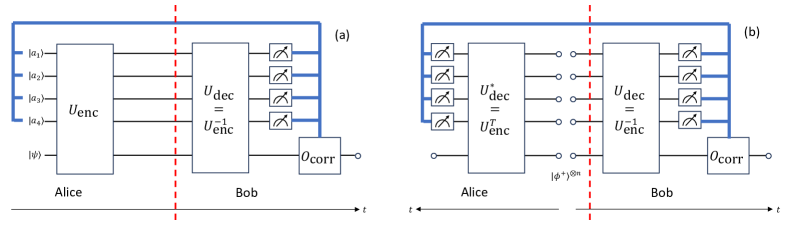
Figure 3: Correspondence between QEC and EPP. (a) One way of implementing quantum error correction to protect a physical quantum state $|\psi\rangle$ to be sent from Alice to Bob. (b) Another equivalent way of sending a physical state $|\psi\rangle$ from Alice to Bob based on shared Bell pairs $|\phi_{2}\rangle^{\otimes n}$ with $n=5$ demonstrated in this figure. Thick blue lines represent classical communication and the vertical red dashed lines separate the two parties, Alice and Bob. Note that on the right hand side of the dashed line (Bob), (a) and (b) are equivalent.

We first consider one way to implement quantum error correction corresponding to (a): We have one physical quantum state $|\psi\rangle$ to protect, and four ancilla qubits are prepared in a certain computational basis state; then an encoding circuit $U_{\mathrm{enc}}$ is applied on all five qubits to create an encoded logical quantum state; at the end the decoding circuit, i.e. the inverse of encoding circuit $U_{\mathrm{dec}}=U_{\mathrm{enc}}^{-1}=U_{\mathrm{enc}}^{\dagger}$ (such that when there is no error the initial state is exactly unchanged), is applied to the encoded quantum state, and four ancilla qubits are measured in computational basis; combined with the knowledge of the ancilla qubits’ initial state and measurement outcomes, we should be able to infer whether there is an error happening in between the encoding and the decoding and can in principle perform error correction on the physical data qubit.

The above mechanism of QEC can be understood in an equivalent approach based on a shared entangled state corresponding to (b): At the beginning several (five in the figure) pure Bell states $|\phi_{2}\rangle$ are prepared by Alice (left) and half of each pair will be sent to Bob (right). Alice measures four out of her five qubits in the computational basis after applying the transpose of encoding circuit in (a) which is also the complex conjugate of the decoding circuit, i.e. $U_{\mathrm{enc}}^{T}=U_{\mathrm{dec}}^{*}$; Bob will apply the same decoding circuit as in (a) and measure four qubits initially entangled with the four qubits measured by Alice; combining the measurement outcomes from Alice and his own, Bob can in principle infer whether certain error has happened during transmission of the five qubits he receives and perform the corresponding error correction operation; the transmission of a physical state $|\psi\rangle$ from Alice to Bob can be achieved a posteriori, supposing Alice measures her remaining qubit in an arbitrary basis which will project Bob’s remaining qubit to an arbitrary state $|\psi\rangle$. Note that in (b) if we only look at the operations on Bob’s side, it is obvious that they are identical to (a), and if Alice does not measure her remaining qubit the entire bipartite process is exactly a 5-to-1 entanglement purification.

Furthermore, we note that the encoding and decoding circuits are Clifford for any stabilizer QEC codes, and thus any $[[n,1,d]]$ stabilizer code corresponds to an $n$-to-1 biCEP. To see this, consider the constructive algorithm of stabilizer encoding [93, 1, 94]. While the technical detail of the algorithm is beyond the scope of this work, it is worth mentioning that the encoding circuit can be constructed by controlled Pauli strings and single-qubit Clifford gates (single-qubit Pauli and Hadamard) only. Therefore, to argue that the encoding circuit is Clifford we only need to show that the controlled Pauli strings are Clifford gates:

Proposition 30.

Any controlled Pauli string applied on $(n+1)$ qubits ($n\geq 1$) is Clifford.

Proof.

Consider an arbitrary controlled Pauli string $(|0\rangle\langle 0|\otimes I+|1\rangle\langle 1|\otimes P)$ with an $n$-qubit Pauli string $P$. We then consider an arbitrary $(n+1)$-qubit Pauli string $P^{(1)}\otimes P^{(n)}$, where $P^{(1)}$ is an arbitrary single-qubit Pauli and $P^{(n)}$ is an arbitrary $n$-qubit Pauli string, and $P^{(1)}$ corresponds to the control qubit. Then we can evaluate the controlled Pauli string conjugate of the arbitrary Pauli string

$$(|0\rangle\langle 0|\otimes I+|1\rangle\langle 1|\otimes P)P^{(1)}\otimes P^{(n)}(|0\rangle\langle 0|\otimes I+|1\rangle\langle 1|\otimes P)$$ (64)

$$= |0\rangle\langle 0|\otimes I(P^{(1)}\otimes P^{(n)})|0\rangle\langle 0|\otimes I+|0\rangle\langle 0|\otimes I(P^{(1)}\otimes P^{(n)})|1\rangle\langle 1|\otimes P$$

$$+|1\rangle\langle 1|\otimes P(P^{(1)}\otimes P^{(n)})|0\rangle\langle 0|\otimes I+|1\rangle\langle 1|\otimes P(P^{(1)}\otimes P^{(n)})|1\rangle\langle 1|\otimes P$$

$$= \langle 0|P^{(1)}|0\rangle|0\rangle\langle 0|\otimes P^{(n)}+\langle 0|P^{(1)}|1\rangle|0\rangle\langle 1|\otimes P^{(n)}P$$

$$+\langle 1|P^{(1)}|0\rangle|1\rangle\langle 0|\otimes PP^{(n)}+\langle 1|P^{(1)}|1\rangle|1\rangle\langle 1|\otimes PP^{(n)}P$$

Recall the representations of $P^{(1)}=I,X,Y,Z$. We see from the last line that the result will always be a Pauli string up to a global phase, which completes the proof. ∎

III.2 Necessary and sufficient condition of universal biCEP for complete BDS sets

Here we prove the universality condition for biCEP (Lemma 7 in the main text), and we separate the proof into two parts for necessity and sufficiency, respectively.

III.2.1 Necessity

If an $n$-to-1 biCEP protocol is universal for a certain class of input states, by definition of universality the output fidelity conditioned on success is one when the input states include at least one noiseless Bell state. Hence, the necessary condition for biCEP to be universal for complete BDS sets can be obtained using the notion of error pattern strings:

Lemma 31 (Necessary condition of universal biCEP).

If an $n$-to-1 biCEP protocol using $n$-qubit Clifford gate $C$ is universal for a complete BDS set, then all single noiseless strings of length $n$ will be transformed by $C$ into harmless strings only.

Proof.

Recall that any complete BDS set $\mathcal{S}$ includes $\phi_{2}$, and satisfies that each of $\Phi^{-},\Psi^{+},\Psi^{-}$ is in the support of at least a BDS in $\mathcal{S}$, where we have rewritten $\Phi^{\pm}=|\phi^{\pm}\rangle\langle\phi^{\pm}|,\Psi^{\pm}=|\psi^{\pm}\rangle\langle\psi^{\pm}|$ for simplicity. Then consider arbitrary combination of $n$ BDS from $\mathcal{S}$ including at least a $\phi_{2}$, and we know that the tensor product of such $n$ BDS equals to $(\phi_{2})^{\otimes n}$ undergoing a unilateral Pauli channel. Obviously the Kraus operators of the unilateral Pauli channel for such input states are single noiseless strings. Moreover, all single noiseless strings are possible when we exhaust all possible input state combinations.

Then suppose an $n$-to-1 biCEP is universal. The output fidelity for such input states should be unity conditioned on success. The output states before measurement are statistical mixtures of Bell state tensor products corresponding to transformation results of single noiseless strings. Unit fidelity of the successful output state requires that single noiseless strings can only be transformed into harmless strings by definition. ∎

III.2.2 Sufficiency

Before proving the sufficient condition, we first provide a formal expression of output fidelity from a biCEP which satisfies Lemma 31 (i.e. candidate of universal biCEP) given the input state:

$$\rho_{in}=\bigotimes_{i=1}^{n}\left[F_{i}\phi_{2}+(1-F_{i})(x_{i}\Psi^{+}+y_{i}\Psi^{-}+z_{i}\Phi^{-})\right]$$ (65)

where $F_{i}$ is the fidelity of the $i$-th input BDS, and $x_{i}+y_{i}+z_{i}=1$ to satisfy normalization of the error probability. Because the tensor product of input Bell diagonal states can be decomposed as a sum of a weighted tensor product of pure Bell states, which correspond to different error pattern strings, here we define the weight function:

Definition 32 (Weight function).

$W:\{\rho_{in}\}\times\overline{\mathcal{P}}_{n}\rightarrow[0,1]$ is the weight function that output the weight of a tensor product of pure Bell states corresponding to a Pauli error string $P\in\overline{\mathcal{P}}_{n}$ in the decomposition of input state $\rho_{in}$.

Remark.

The weight function satisfies the following property of normalization: $\sum_{P\in\overline{\mathcal{P}}_{n}}W(\rho_{in},P)=1$, $\forall\rho_{in}$. Without loss of clarity, in the following we will omit the input state in weight function.

We would like to express the biCEP output according to the underlying transformation of Pauli strings by the corresponding Clifford. To make description concise, we define the following types of Pauli strings:

Definition 33 (Type 1 ($T_{1}$)).

A Type 1 ($T_{1}$) Pauli string has the form of $I\otimes P,\ P\in\overline{\mathcal{P}}_{n-1}$.

Definition 34 (Type 2 ($T_{2}$)).

A Type 2 ($T_{2}$) Pauli string has the form of $\{X,Y,Z\}\otimes P,\ P\in\overline{\mathcal{P}}_{n-1}$.

Then we have the output fidelity and success probability from an universal biCEP candidate:

Lemma 35 (Universal biCEP output).

If a biCEP protocol satisfies the necessary condition of universal for general BDS input, then the success probability and output fidelity conditioned on success are given as follows

$$p_{suss}= \sum_{s\in T_{1},s\rightarrow s^{\prime}\in\mathrm{Correct}}W(s)+\sum_{t\in T_{2},t\rightarrow t^{\prime}\in\mathrm{Correct}}W(t)+\sum_{r\in T_{2},r\rightarrow r^{\prime}\in\mathrm{Undetectable}}W(r),$$ (66)

$$F_{out}= \frac{\sum_{s\in T_{1},s\rightarrow s^{\prime}\in\mathrm{Correct}}W(s)+\sum_{t\in T_{2},t\rightarrow t^{\prime}\in\mathrm{Correct}}W(t)}{\sum_{s\in T_{1},s\rightarrow s^{\prime}\in\mathrm{Correct}}W(s)+\sum_{t\in T_{2},t\rightarrow t^{\prime}\in\mathrm{Correct}}W(t)+\sum_{r\in T_{2},r\rightarrow r^{\prime}\in\mathrm{Undetectable}}W(r)}$$

$$= \frac{1}{1+\frac{\sum_{r\in T_{2},r\rightarrow r^{\prime}\in\mathrm{Undetectable}}W(r)}{\sum_{s\in T_{1},s\rightarrow s^{\prime}\in\mathrm{Correct}}W(s)+\sum_{t\in T_{2},t\rightarrow t^{\prime}\in\mathrm{Correct}}W(t)}}.$$

Proof.

According to the assumption that the biCEP protocol is an universal candidate for a complete BDS set, $T_{1}$ Pauli strings are all single noiseless strings and thus will only be transformed to harmless strings following Lemma 31; $T_{2}$ Pauli strings can be transformed to either harmless or undetectable strings. Then the expressions follow naturally from the definition of success criterion of biCEP protocols. ∎

Equipped with the above preparation, we prove the sufficient condition of universality as follows:

Lemma 36 (Sufficient condition of universal biCEP).

If an $n$-qubit Clifford gate $C$ transforms all single noiseless strings of length $n$ into harmless strings only, then the $n$-to-1 biCEP protocol using $C$ is universal for all complete BDS sets.

Proof.

In this proof we first find the lower bound of successful output fidelity, and then show that this lower bound is always not less than the highest input fidelity as long as all input fidelities are greater than $1/2$, which is one requirement in the definition of complete BDS set.

It is obvious from Lemma 35 that:

$$F_{out}\geq\frac{1}{1+\frac{\max_{\{F_{m}\}}\left\{\sum_{r\in T_{2},r\rightarrow r^{\prime}\in\mathrm{Undetectable}}W(r)\right\}}{\min_{\{F_{m}\}}\left\{\sum_{s\in T_{1},s\rightarrow s^{\prime}\in\mathrm{Correct}}W(s)\right\}+\min_{\{F_{m}\}}\left\{\sum_{t\in T_{2},t\rightarrow t^{\prime}\in\mathrm{Correct}}W(t)\right\}}}$$ (67)

where $\max(\min)_{\{F_{m}\}}\{\cdot\}$ means the highest (lowest) possible value of a certain object given fixed input state fidelities $\{F_{m}\}$. The highest and lowest possible values involved can be found by considering “worst case scenarios”:

1. $\sum_{s\in T_{1},s\rightarrow s^{\prime}\in\mathrm{Correct}}W(s)\geq\prod_{m=1}^{n}F_{m}$, where the right hand side equals the probability of the tensor product of $n$ noiseless $\phi_{2}$’s which corresponds to the identity string. The identity will always be transformed back to identity which is a correct string, and the worst case scenario is when there is no other type 1 string transformed to correct string.

2. $\sum_{t\in T_{2},t\rightarrow t^{\prime}\in\mathrm{Correct}}W(t)\geq 0$. There is no guarantee that there are type 2 strings which will be transformed to correct strings, thus the worst case scenario is that no type 2 string is transformed to correct strings which gives the value 0.

3. $\sum_{r\in T_{2},r\rightarrow r^{\prime}\in\mathrm{Undetectable}}W(r)\leq\prod_{m=1}^{n}(1-F_{m})$. Suppose the rank of $m$-th input BDS is $r_{m}$. We have in total $\prod_{m=1}^{n}(r_{m}-1)$ type 2 strings which are not single noiseless strings. These strings are possible to be transformed to undetectable strings. As there are $3\times 2^{n-1}$ undetectable strings, as long as $\prod_{m=1}^{n}(r_{m}-1)\leq 3\times 2^{n-1}$ the worst case scenario would be that all these $\prod_{m=1}^{n}(r_{m}-1)$ type 2 strings are transformed to undetectable strings.

With above bounds, we have the explicit lower bound of output fidelity for fixed input state fidelities $\{F_{m}\}$

$$F_{out}\geq\frac{\prod_{m=1}^{n}F_{m}}{\prod_{m=1}^{n}F_{m}+\prod_{m=1}^{n}(1-F_{m})}=F_{out}^{\min}$$ (68)

which is independent of the previously chosen $i$-th input Bell state, as expected from the arbitrariness of the choice.

Now we move on to prove that this lower bound is in fact guaranteed to be higher than the highest input fidelity $F_{\max}=\max[\{F_{m}\}]$ if $F_{m}\geq 1/2$. We rewrite the lower bound expression as

$$F_{out}^{\min}= F_{\max}\frac{\prod_{m\neq m_{\max}}F_{m}}{F_{\max}\prod_{m\neq m_{\max}}F_{m}+(1-F_{\max})\prod_{m\neq m_{\max}}(1-F_{m})}$$ (69)

$$= F_{\max}\frac{F_{\max}\prod_{m\neq m_{\max}}F_{m}+(1-F_{\max})\prod_{m\neq m_{\max}}F_{m}}{F_{\max}\prod_{m\neq m_{\max}}F_{m}+(1-F_{\max})\prod_{m\neq m_{\max}}(1-F_{m})}\geq F_{\max}$$

where $m_{\max}$ refers to the index of the input Bell state with highest fidelity $F_{\max}$, and the inequality holds because $1-F_{m}\leq F_{m}$ if $F_{m}\geq 1/2$. In this way, the statement is proved. ∎

III.2.3 Example usage of the necessary and sufficient condition

Here we demonstrate the effectiveness of the universal condition by proving the universal property of DEJMPS (a 2-to-1 biCEP with $C=\mathrm{CNOT}$) protocol through Pauli string checking only, which is proved elsewhere [75] analytically.

Proposition 37.

DEJMPS protocol is universal for bit-flipped Bell states (in the form of $\rho_{X}=F\phi_{2}+(1-F)\Psi^{+}$) with fidelity higher than 1/2 as input, but not universal for all entangled isotropic states.

Proof.

Notice that the set of bit-flipped Bell states is not a complete BDS set, the universality condition also needs to be modified a bit from the conditions proved above, and we only need to require that all Pauli strings with at least one identity operator while all remaining Pauli operators being $X$ can be transformed by the Clifford gate to harmless strings. The proof of this modification is very similar to the above proofs, so is omitted. Now we only need to check the transformation of the following 2-qubit Pauli strings by CNOT:

$$I\otimes I\rightarrow I\otimes I,\ X\otimes I\rightarrow X\otimes X,\ I\otimes X\rightarrow I\otimes X,$$ (70)

and the transformed Pauli strings are obviously all harmless strings so DEJMPS is indeed universal for bit-flipped Bell states. Then notice that the set of all entangled isotropic states is a complete BDS set. We need to evaluate the transformation of some additional Pauli strings:

$$I\otimes Y\rightarrow Z\otimes Y,\ I\otimes Z\rightarrow Z\otimes Z,$$ (71)

$$Y\otimes I\rightarrow Y\otimes X,\ Z\otimes I\rightarrow Z\otimes I.$$

Notice that $Z\otimes I$ which is unchanged is not a harmless string. This means that DEJMPS cannot stay universal for all entangled isotropic states. ∎

III.3 Proof of no universal biCEP protocol

Here we prove the Proposition 8 in the main text.

Proposition 38.

For any $\mathcal{S}\in\mathfrak{C}$ and $n\geq 2$, $n$-to-1 biCEP protocols cannot be universal for $\mathcal{S}$.

Proof.

We utilize the fact that Pauli string transformation via Clifford conjugate is an automorphism of Pauli group, which means that any group structure must be preserved, specifically group multiplication. Thus we examine group structures within single noiseless strings and harmless strings.

Firstly, we can make the following observations about single noiseless strings:

• They include $n$ Pauli subgroups which are isomorphic to $(n-1)$-qubit Pauli group $\overline{\mathcal{P}}_{n-1}$, in form of $I_{i}\otimes\left(\bigotimes_{j\neq i}P_{j}\right),\ P_{j}\in\overline{\mathcal{P}}_{1}$ where the Pauli operator on the $i$-th qubit is fixed to be identity.

• These subgroups are necessarily overlapping, and any $2\leq m\leq n$ of these subgroups have $4^{n-m}$ overlapping terms which are isomorphic to $(n-m)$-qubit Pauli group $\overline{\mathcal{P}}_{n-m}$. This can be verified by calculating the number of total Pauli strings according to the overlapping structure of these $n$ subgroups:

  $$\sum_{k=1}^{n}(-1)^{k+1}\binom{n}{k}4^{n-k}=4^{n}-3^{n}$$ (72)

  according to inclusion-exclusion principle. It is clear that this number equals the number of single noiseless strings. Meanwhile, all Pauli strings in such subgroups are single noiseless strings according to definition, thus we have shown that single noiseless strings indeed possess the structure with these subgroups.

We can see that $P_{h}^{(n)}$ at least contains one such set of Pauli strings, i.e. $S_{0}\equiv\{I\otimes P,\ P\in\overline{\mathcal{P}}_{n-1}\}$. We thus prove the theorem by contradiction through the attempt of constructing other such sets via replacing strings in $S_{0}$ with other harmless strings not in $S_{0}$.

Suppose we can construct a different set satisfying same properties as $S_{0}$. The replacing strings from outside $S_{0}$ can only have one type or three types of Pauli operators on their first site, because supposing there are only two types of Pauli operators on the first site, product between non-$S_{0}$ strings can get the third type of Pauli operator on the first site, which is obviously outside the set thus contradicting the assumption. Furthermore, if the replacing strings have only one type of non-identity Pauli on the first site, then there are necessarily $4^{n-1}/2$ original $S_{0}$ strings in the newly constructed set with $4^{n-1}$ elements in total. This can be seen as follows: Suppose that there are $m$ $S_{0}$ strings including the identity string remaining; then as the $m$ strings are different, multiplication of any non-$S_{0}$ string and remaining $S_{0}$ strings will produce $m-1$ non-$S_{0}$ strings different from the one involved in multiplication. This means that there should be at least $m$ added non-$S_{0}$ strings. Meanwhile, closed-ness under multiplication requires that there are at most $m$ added non-$S_{0}$ strings, because for $l$ different non-$S_{0}$ strings with same type of Pauli on the first site there are at least $l$ different $S_{0}$ strings, including identity string, which will be generated from multiplication between the $l$ non-$S_{0}$ strings. Therefore, from the requirement on the size of newly constructed set we have that $m+m=4^{n-1}\Leftrightarrow m=4^{n-1}/2$. Similarly, suppose there are three different first-site Pauli operators among added non-$S_{0}$ strings. the multiplication between added strings and remaining $S_{0}$ strings, together with multiplication between added strings with same type of first-site Pauli requires that the number of strings with any first-site Pauli to be equal, i.e. $4n=4^{n-1}\Leftrightarrow m=4^{n-2}$.

Suppose we can construct another subset of harmless strings that share same properties with $S_{0}$. The added string with non-identity first-site Pauli should not have same last $(n-1)$-qubit Pauli string as that of any remaining $S_{0}$ string, because otherwise the multiplication of the non-$S_{0}$ string and $S_{0}$ string can get outside harmless string. This means that we can divide the constructed set into two non-intersecting subsets, of which one is $S_{0}$ subgroup $I\otimes\{P^{(n-1)}\}$ and the other is $\{X,Y,Z\}\otimes p_{X,Y,Z}\{P^{(n-1)}\}$, where $p_{X,Y,Z}\notin\{P^{(n-1)}\}$ and $p_{X,Y,Z}\{P^{(n-1)}\}$ are cosets of $\overline{\mathcal{P}}_{n-1}$ subgroup $\{P^{(n-1)}\}$. Then the $4^{n-1}$ strings in the constructed set actually have all $4^{n-1}$ different $(n-1)$-qubit Pauli strings on their last $n-1$ sites, i.e. other than the leftmost Pauli. Therefore, the first part $I\otimes\{P^{(n-1)}\}$ should contain all $2^{n-1}=4^{(n-1)/2}$ correct strings. Now we come across an obvious contradiction that any $2\leq m\leq n$ of these constructed subgroups have at least have $4^{(n-1)/2}$ overlapping terms which are the correct strings as mentioned above, while they should have $4^{n-m}$ overlapping terms which are isomorphic to $(n-m)$-qubit Pauli group $\overline{\mathcal{P}}_{n-m}$.

In this way, we know that such construction is impossible, i.e. we cannot find a way to construct $n$ different but overlapping harmless string subsets to satisfy the properties of single noiseless strings. This contradicts with the assumption that there exists a universal biCEP, which concludes that there does not exist universal biCEP for any integer $n>1$. ∎

III.4 Bilocal Clifford protocols that are universal with ordered fidelity are necessarily trivial

Our definition of universality (Definition 1 in the main text) only requires non-decreasing output fidelity in comparison with highest input fidelity, it is thus possible that the output fidelity is always equal to the highest input fidelity. Obviously such result can be achieved by Clifford which can be decomposed into the form $I\otimes C_{n-1},\ C_{n-1}\in\mathcal{C}_{n-1}$ supposing we have ordered fidelity and always put the input state with highest fidelity on the first site and do not measure it. We call such universal biCEP protocols trivially universal. In the following we prove the Proposition 10 in the main text, that given ordered fidelity, all universal biCEP must be trivial. Here we rephrase the proposition in terms of Pauli string transformation.

Proposition 39.

If the underlying Clifford gate of a biCEP maps Pauli strings in the form of $I\otimes P$ where $P$ is arbitrary $(n-1)$-qubit Pauli string to harmless strings only, then for input states $\rho_{1},\dots,\rho_{n}$ the output fidelity equals the fidelity of $\rho_{1}$, where we keep the qubits of $\rho_{1}$ unmeasured.

Proof.

Consider Pauli strings $X\otimes I_{n-1}$, $Y\otimes I_{n-1}$, and $Z\otimes I_{n-1}$. Each of these three strings commutes with all of strings of the form $I\otimes P$, where $P\in\overline{\mathcal{P}}_{n-1}$. We have shown earlier in the proof of no universal biCEP that if the set $\{I\otimes P:\,P\in\overline{\mathcal{P}}_{n-1}\}$ is mapped to harmless strings, then it must be mapped to a set that contains all strings of the form $I\otimes\{I,Z\}^{\otimes n-1}$, i.e. correct strings.

Since Clifford conjugation preserves commutation relations, we must have that all three of $X\otimes I_{n-1}$, $Y\otimes I_{n-1}$, and $Z\otimes I_{n-1}$ are mapped to undetectable strings. This can be shown as follows: Suppose that there exist one of them mapped to harmless string, then it can only be mapped to incorrect string (all correct strings are mapped to from $I\otimes P$); incorrect strings have at least one $X$ or $Y$ among their last $n-1$ Pauli operators, while none correct strings has $X$ or $Y$ among their last $n-1$ Pauli operators; this means that any incorrect string cannot commute with all correct strings; however, $X\otimes I_{n-1}$, $Y\otimes I_{n-1}$, and $Z\otimes I_{n-1}$ commute with any $I\otimes P$, therefore even after Clifford conjugation they should still commute, and this can never be achieved if $X\otimes I_{n-1}$, $Y\otimes I_{n-1}$, and $Z\otimes I_{n-1}$ are mapped to incorrect strings, leading to contradiction.

Furthermore, since Clifford conjugation preserves multiplication, we find that for any $P\in\overline{\mathcal{P}}_{n-1}$, if $I\otimes P$ is mapped to a correct string, $X\otimes P$, $Y\otimes P$, and $Z\otimes P$ are mapped to undetectable strings. Conversely, if $I\otimes P$ is mapped to an incorrect string, then $X\otimes P$, $Y\otimes P$, and $Z\otimes P$ are mapped to incorrect strings. Now we can calculate the output fidelity of a universal biCEP via Lemma 35, where

$$\sum_{r\in T_{2},r\rightarrow r^{\prime}\in\mathrm{Undetectable}}W(r) =\sum_{I\otimes P\rightarrow\{P_{c}^{(n)}\}}\left[W(X\otimes P)+W(Y\otimes P)+W(Z\otimes P)\right],$$ (73)

$$\sum_{s\in T_{1},s\rightarrow s^{\prime}\in\mathrm{Correct}}W(s) =\sum_{I\otimes P\rightarrow\{P_{c}^{(n)}\}}W(I\otimes P),$$ (74)

$$\sum_{t\in T_{2},t\rightarrow t^{\prime}\in\mathrm{Correct}}W(t) =0.$$ (75)

Notice that for any $P$ we always have $W(X\otimes P)+W(Y\otimes P)+W(Z\otimes P)=(1-F_{1})W(I\otimes P)$. It is then easy to see that $F_{out}=F_{1}$. ∎

References

- Gottesman [1997] D. Gottesman, Stabilizer codes and quantum error correction (California Institute of Technology, 1997).
- Jiang et al. [2009] L. Jiang, J. M. Taylor, K. Nemoto, W. J. Munro, R. Van Meter, and M. D. Lukin, Quantum repeater with encoding, Physical Review A 79, 032325 (2009).
- Munro et al. [2010] W. Munro, K. Harrison, A. Stephens, S. Devitt, and K. Nemoto, From quantum multiplexing to high-performance quantum networking, Nature Photonics 4, 792 (2010).
- Fowler et al. [2010] A. G. Fowler, D. S. Wang, C. D. Hill, T. D. Ladd, R. Van Meter, and L. C. Hollenberg, Surface code quantum communication, Physical Review Letters 104, 180503 (2010).
- Muralidharan et al. [2014] S. Muralidharan, J. Kim, N. Lütkenhaus, M. D. Lukin, and L. Jiang, Ultrafast and fault-tolerant quantum communication across long distances, Physical Review Letters 112, 250501 (2014).
- Bennett et al. [1996a] C. H. Bennett, G. Brassard, S. Popescu, B. Schumacher, J. A. Smolin, and W. K. Wootters, Purification of noisy entanglement and faithful teleportation via noisy channels, Physical Review Letters 76, 722 (1996a).
- Deutsch et al. [1996] D. Deutsch, A. Ekert, R. Jozsa, C. Macchiavello, S. Popescu, and A. Sanpera, Quantum privacy amplification and the security of quantum cryptography over noisy channels, Physical Review Letters 77, 2818 (1996).
- Bennett et al. [1996b] C. H. Bennett, D. P. DiVincenzo, J. A. Smolin, and W. K. Wootters, Mixed-state entanglement and quantum error correction, Physical Review A 54, 3824 (1996b).
- Dür and Briegel [2007] W. Dür and H. J. Briegel, Entanglement purification and quantum error correction, Reports on Progress in Physics 70, 1381 (2007).
- Horodecki et al. [2009] R. Horodecki, P. Horodecki, M. Horodecki, and K. Horodecki, Quantum entanglement, Reviews of Modern Physics 81, 865 (2009).
- Pan et al. [2001] J.-W. Pan, C. Simon, Č. Brukner, and A. Zeilinger, Entanglement purification for quantum communication, Nature 410, 1067 (2001).
- Pan et al. [2003] J.-W. Pan, S. Gasparoni, R. Ursin, G. Weihs, and A. Zeilinger, Experimental entanglement purification of arbitrary unknown states, Nature 423, 417 (2003).
- Hu et al. [2021] X.-M. Hu, C.-X. Huang, Y.-B. Sheng, L. Zhou, B.-H. Liu, Y. Guo, C. Zhang, W.-B. Xing, Y.-F. Huang, C.-F. Li, et al., Long-distance entanglement purification for quantum communication, Physical Review Letters 126, 010503 (2021).
- Ecker et al. [2021] S. Ecker, P. Sohr, L. Bulla, M. Huber, M. Bohmann, and R. Ursin, Experimental single-copy entanglement distillation, Physical Review Letters 127, 040506 (2021).
- Reichle et al. [2006] R. Reichle, D. Leibfried, E. Knill, J. Britton, R. B. Blakestad, J. D. Jost, C. Langer, R. Ozeri, S. Seidelin, and D. J. Wineland, Experimental purification of two-atom entanglement, Nature 443, 838 (2006).
- Kalb et al. [2017] N. Kalb, A. A. Reiserer, P. C. Humphreys, J. J. Bakermans, S. J. Kamerling, N. H. Nickerson, S. C. Benjamin, D. J. Twitchen, M. Markham, and R. Hanson, Entanglement distillation between solid-state quantum network nodes, Science 356, 928 (2017).
- Yan et al. [2022] H. Yan, Y. Zhong, H.-S. Chang, A. Bienfait, M.-H. Chou, C. R. Conner, É. Dumur, J. Grebel, R. G. Povey, and A. N. Cleland, Entanglement purification and protection in a superconducting quantum network, Physical Review Letters 128, 080504 (2022).
- Raussendorf et al. [2003] R. Raussendorf, D. E. Browne, and H. J. Briegel, Measurement-based quantum computation on cluster states, Physical Review A 68, 022312 (2003).
- Cacciapuoti et al. [2019] A. S. Cacciapuoti, M. Caleffi, F. Tafuri, F. S. Cataliotti, S. Gherardini, and G. Bianchi, Quantum internet: Networking challenges in distributed quantum computing, IEEE Network 34, 137 (2019).
- Cuomo et al. [2020] D. Cuomo, M. Caleffi, and A. S. Cacciapuoti, Towards a distributed quantum computing ecosystem, IET Quantum Communication 1, 3 (2020).
- Proctor et al. [2018] T. J. Proctor, P. A. Knott, and J. A. Dunningham, Multiparameter estimation in networked quantum sensors, Physical review letters 120, 080501 (2018).
- Zhang and Zhuang [2021] Z. Zhang and Q. Zhuang, Distributed quantum sensing, Quantum Science and Technology 6, 043001 (2021).
- Kimble [2008] H. J. Kimble, The quantum internet, Nature 453, 1023 (2008).
- Wehner et al. [2018] S. Wehner, D. Elkouss, and R. Hanson, Quantum internet: A vision for the road ahead, Science 362, eaam9288 (2018).
- Bennett et al. [1993] C. H. Bennett, G. Brassard, C. Crépeau, R. Jozsa, A. Peres, and W. K. Wootters, Teleporting an unknown quantum state via dual classical and Einstein-Podolsky-Rosen channels, Physical Review Letters 70, 1895 (1993).
- Dür et al. [1999] W. Dür, H.-J. Briegel, J. I. Cirac, and P. Zoller, Quantum repeaters based on entanglement purification, Physical Review A 59, 169 (1999).
- Dür and Briegel [2003] W. Dür and H.-J. Briegel, Entanglement purification for quantum computation, Physical Review Letters 90, 067901 (2003).
- Martinis [2015] J. M. Martinis, Qubit metrology for building a fault-tolerant quantum computer, npj Quantum Information 1, 1 (2015).
- Harper et al. [2020] R. Harper, S. T. Flammia, and J. J. Wallman, Efficient learning of quantum noise, Nature Physics 16, 1184 (2020).
- Eisert et al. [2020] J. Eisert, D. Hangleiter, N. Walk, I. Roth, D. Markham, R. Parekh, U. Chabaud, and E. Kashefi, Quantum certification and benchmarking, Nature Reviews Physics 2, 382 (2020).
- Kliesch and Roth [2021] M. Kliesch and I. Roth, Theory of quantum system certification, PRX Quantum 2, 010201 (2021).
- Klimov et al. [2018] P. Klimov, J. Kelly, Z. Chen, M. Neeley, A. Megrant, B. Burkett, R. Barends, K. Arya, B. Chiaro, Y. Chen, et al., Fluctuations of energy-relaxation times in superconducting qubits, Physical Review Letters 121, 090502 (2018).
- Burnett et al. [2019] J. J. Burnett, A. Bengtsson, M. Scigliuzzo, D. Niepce, M. Kudra, P. Delsing, and J. Bylander, Decoherence benchmarking of superconducting qubits, npj Quantum Information 5, 54 (2019).
- Chitambar et al. [2014] E. Chitambar, D. Leung, L. Mančinska, M. Ozols, and A. Winter, Everything you always wanted to know about LOCC (but were afraid to ask), Communications in Mathematical Physics 328, 303 (2014).
- Rains [1997] E. M. Rains, Entanglement purification via separable superoperators, arXiv preprint quant-ph/9707002 (1997).
- Rains [1999] E. M. Rains, Rigorous treatment of distillable entanglement, Physical Review A 60, 173 (1999).
- [37] See Supplemental Material (SM) for more technical details, which includes Ref. [23, 24, 25, 70, 19, 20, 22, 1, 2, 3, 4, 5, 6, 7, 8, 9, 10, 71, 72, 73, 74, 28, 29, 30, 31, 32, 33, 75, 76, 77, 78, 79, 80, 81, 82, 35, 83, 36, 84, 85, 41, 86, 87, 88, 89, 90, 91, 42, 47, 92, 93, 94].
- Note [1] We note that although there exist entangled states with fidelity below 1/2 [95, 96], they can always be transformed into states with fidelity above 1/2 through LOCC [97, 98]. However, admittedly the filtering operations are state-dependent, and it assumes a priori knowledge of state. Nevertheless, the 1/2 fidelity threshold is well motivated by requirement of non-trivial quantum teleportation [99].
- Gurvits [2003] L. Gurvits, Classical deterministic complexity of Edmonds’ problem and quantum entanglement, in Proceedings of the thirty-fifth annual ACM Symposium on Theory of Computing (2003) pp. 10–19.
- Ioannou [2006] L. M. Ioannou, Computational complexity of the quantum separability problem, arXiv preprint quant-ph/0603199 (2006).
- De Vicente [2006] J. I. De Vicente, Separability criteria based on the Bloch representation of density matrices, arXiv preprint quant-ph/0607195 (2006).
- Jansen et al. [2022] S. Jansen, K. Goodenough, S. de Bone, D. Gijswijt, and D. Elkouss, Enumerating all bilocal Clifford distillation protocols through symmetry reduction, Quantum 6, 715 (2022).
- Aaronson and Gottesman [2004] S. Aaronson and D. Gottesman, Improved simulation of stabilizer circuits, Physical Review A 70, 052328 (2004).
- Selinger [2015] P. Selinger, Generators and relations for n-qubit Clifford operators, Logical Methods in Computer Science 11 (2015).
- Maslov and Roetteler [2018] D. Maslov and M. Roetteler, Shorter stabilizer circuits via Bruhat decomposition and quantum circuit transformations, IEEE Transactions on Information Theory 64, 4729 (2018).
- Bravyi and Maslov [2021] S. Bravyi and D. Maslov, Hadamard-free circuits expose the structure of the Clifford group, IEEE Transactions on Information Theory 67, 4546 (2021).
- Aschauer [2005] H. Aschauer, Quantum communication in noisy environments (LMU Munich, 2005).
- Dür et al. [2005] W. Dür, M. Hein, J. I. Cirac, and H.-J. Briegel, Standard forms of noisy quantum operations via depolarization, Physical Review A 72, 052326 (2005).
- Emerson et al. [2007] J. Emerson, M. Silva, O. Moussa, C. Ryan, M. Laforest, J. Baugh, D. G. Cory, and R. Laflamme, Symmetrized characterization of noisy quantum processes, Science 317, 1893 (2007).
- Dankert et al. [2009] C. Dankert, R. Cleve, J. Emerson, and E. Livine, Exact and approximate unitary 2-designs and their application to fidelity estimation, Physical Review A 80, 012304 (2009).
- Muralidharan et al. [2016] S. Muralidharan, L. Li, J. Kim, N. Lütkenhaus, M. D. Lukin, and L. Jiang, Optimal architectures for long distance quantum communication, Scientific Reports 6, 20463 (2016).
- Azuma et al. [2023] K. Azuma, S. E. Economou, D. Elkouss, P. Hilaire, L. Jiang, H.-K. Lo, and I. Tzitrin, Quantum repeaters: From quantum networks to the quantum internet, Reviews of Modern Physics 95, 045006 (2023).
- Cong et al. [2022] I. Cong, H. Levine, A. Keesling, D. Bluvstein, S.-T. Wang, and M. D. Lukin, Hardware-efficient, fault-tolerant quantum computation with Rydberg atoms, Physical Review X 12, 021049 (2022).
- Note [2] We note that Ref. [53] considers error conversion for Rydberg state, while Rydberg state is in general not directly used for quantum memory.
- Mirrahimi et al. [2014] M. Mirrahimi, Z. Leghtas, V. V. Albert, S. Touzard, R. J. Schoelkopf, L. Jiang, and M. H. Devoret, Dynamically protected cat-qubits: a new paradigm for universal quantum computation, New Journal of Physics 16, 045014 (2014).
- Lescanne et al. [2020] R. Lescanne, M. Villiers, T. Peronnin, A. Sarlette, M. Delbecq, B. Huard, T. Kontos, M. Mirrahimi, and Z. Leghtas, Exponential suppression of bit-flips in a qubit encoded in an oscillator, Nature Physics 16, 509 (2020).
- Grimm et al. [2020] A. Grimm, N. E. Frattini, S. Puri, S. O. Mundhada, S. Touzard, M. Mirrahimi, S. M. Girvin, S. Shankar, and M. H. Devoret, Stabilization and operation of a Kerr-cat qubit, Nature 584, 205 (2020).
- Brandão and Eisert [2008] F. G. Brandão and J. Eisert, Correlated entanglement distillation and the structure of the set of undistillable states, Journal of Mathematical Physics 49 (2008).
- Buscemi and Datta [2010] F. Buscemi and N. Datta, Distilling entanglement from arbitrary resources, Journal of Mathematical Physics 51 (2010).
- Waeldchen et al. [2016] S. Waeldchen, J. Gertis, E. T. Campbell, and J. Eisert, Renormalizing entanglement distillation, Physical Review Letters 116, 020502 (2016).
- Murao et al. [1998] M. Murao, M. Plenio, S. Popescu, V. Vedral, and P. Knight, Multiparticle entanglement purification protocols, Physical Review A 57, R4075 (1998).
- Maneva and Smolin [2002] E. N. Maneva and J. A. Smolin, Improved two-party and multi-party purification protocols, Contemporary Mathematics 305, 203 (2002).
- Dür et al. [2003] W. Dür, H. Aschauer, and H.-J. Briegel, Multiparticle entanglement purification for graph states, Physical Review Letters 91, 107903 (2003).
- Aschauer et al. [2005] H. Aschauer, W. Dür, and H.-J. Briegel, Multiparticle entanglement purification for two-colorable graph states, Physical Review A 71, 012319 (2005).
- Kruszynska et al. [2006] C. Kruszynska, A. Miyake, H. J. Briegel, and W. Dür, Entanglement purification protocols for all graph states, Physical Review A 74, 052316 (2006).
- Bravyi and Kitaev [2005] S. Bravyi and A. Kitaev, Universal quantum computation with ideal Clifford gates and noisy ancillas, Physical Review A 71, 022316 (2005).
- Bravyi and Haah [2012] S. Bravyi and J. Haah, Magic-state distillation with low overhead, Physical Review A 86, 052329 (2012).
- Vollbrecht and Werner [2001] K. G. H. Vollbrecht and R. F. Werner, Entanglement measures under symmetry, Physical Review A 64, 062307 (2001).
- Chruściński and Kossakowski [2006] D. Chruściński and A. Kossakowski, Multipartite invariant states. I. Unitary symmetry, Physical Review A 73, 062314 (2006).
- Gottesman and Chuang [1999] D. Gottesman and I. L. Chuang, Demonstrating the viability of universal quantum computation using teleportation and single-qubit operations, Nature 402, 390 (1999).
- Lütkenhaus et al. [1999] N. Lütkenhaus, J. Calsamiglia, and K.-A. Suominen, Bell measurements for teleportation, Physical Review A 59, 3295 (1999).
- Briegel et al. [1998] H.-J. Briegel, W. Dür, J. I. Cirac, and P. Zoller, Quantum repeaters: the role of imperfect local operations in quantum communication, Physical Review Letters 81, 5932 (1998).
- Rozpędek et al. [2018] F. Rozpędek, T. Schiet, D. Elkouss, A. C. Doherty, S. Wehner, et al., Optimizing practical entanglement distillation, Physical Review A 97, 062333 (2018).
- Krastanov et al. [2019] S. Krastanov, V. V. Albert, and L. Jiang, Optimized entanglement purification, Quantum 3, 123 (2019).
- Zang et al. [2024] A. Zang et al., In preparation (2024).
- Khatri [2021] S. Khatri, Policies for elementary links in a quantum network, Quantum 5, 537 (2021).
- Santra et al. [2019] S. Santra, L. Jiang, and V. S. Malinovsky, Quantum repeater architecture with hierarchically optimized memory buffer times, Quantum Science and Technology 4, 025010 (2019).
- Zang et al. [2023] A. Zang, X. Chen, A. Kolar, J. Chung, M. Suchara, T. Zhong, and R. Kettimuthu, Entanglement distribution in quantum repeater with purification and optimized buffer time, in IEEE INFOCOM 2023 - IEEE Conference on Computer Communications Workshops (2023) pp. 1–6.
- Chakraborty et al. [2019] K. Chakraborty, F. Rozpedek, A. Dahlberg, and S. Wehner, Distributed routing in a quantum internet, arXiv preprint arXiv:1907.11630 (2019).
- Kolar et al. [2022] A. Kolar, A. Zang, J. Chung, M. Suchara, and R. Kettimuthu, Adaptive, continuous entanglement generation for quantum networks, in IEEE INFOCOM 2022-IEEE Conference on Computer Communications Workshops (IEEE, 2022) pp. 1–6.
- Iñesta and Wehner [2023] Á. G. Iñesta and S. Wehner, Performance metrics for the continuous distribution of entanglement in multiuser quantum networks, Physical Review A 108, 052615 (2023).
- Ghaderibaneh et al. [2022] M. Ghaderibaneh, H. Gupta, C. Ramakrishnan, and E. Luo, Pre-distribution of entanglements in quantum networks, in 2022 IEEE International Conference on Quantum Computing and Engineering (QCE) (IEEE, 2022) pp. 426–436.
- Cirac et al. [2001] J. I. Cirac, W. Dür, B. Kraus, and M. Lewenstein, Entangling operations and their implementation using a small amount of entanglement, Physical Review Letters 86, 544 (2001).
- Rains [2001] E. M. Rains, A semidefinite program for distillable entanglement, IEEE Transactions on Information Theory 47, 2921 (2001).
- DiVincenzo et al. [2002] D. P. DiVincenzo, D. W. Leung, and B. M. Terhal, Quantum data hiding, IEEE Transactions on Information Theory 48, 580 (2002).
- Nielsen and Chuang [2010] M. A. Nielsen and I. L. Chuang, Quantum computation and quantum information (Cambridge University Press, 2010).
- Rudolph [2005] O. Rudolph, Further results on the cross norm criterion for separability, Quantum Information Processing 4, 219 (2005).
- Chen and Wu [2002] K. Chen and L.-A. Wu, A matrix realignment method for recognizing entanglement, arXiv preprint quant-ph/0205017 (2002).
- Egorychev [1984] G. P. Egorychev, Integral representation and the computation of combinatorial sums, Vol. 59 (American Mathematical Soc., 1984).
- Prudnikov et al. [1988] A. P. Prudnikov, Y. A. Brychkov, O. I. Marichev, and R. H. Romer, Integrals and Series, American Journal of Physics 56, 957 (1988).
- Olver et al. [2010] F. W. Olver, D. W. Lozier, R. Boisvert, and C. W. Clark, NIST handbook of mathematical functions (Cambridge university press, 2010).
- Hostens et al. [2004] E. Hostens, J. Dehaene, and B. De Moor, The equivalence of two approaches to the design of entanglement distillation protocols, arXiv preprint quant-ph/0406017 (2004).
- Cleve and Gottesman [1997] R. Cleve and D. Gottesman, Efficient computations of encodings for quantum error correction, Physical Review A 56, 76 (1997).
- Gaitan [2008] F. Gaitan, Quantum error correction and fault tolerant quantum computing (CRC Press, 2008).
- Badziag et al. [2000] P. Badziag, M. Horodecki, P. Horodecki, and R. Horodecki, Local environment can enhance fidelity of quantum teleportation, Physical Review A 62, 012311 (2000).
- Verstraete and Verschelde [2002] F. Verstraete and H. Verschelde, Fidelity of mixed states of two qubits, Physical Review A 66, 022307 (2002).
- Horodecki et al. [1997] M. Horodecki, P. Horodecki, and R. Horodecki, Inseparable two spin-1/2 density matrices can be distilled to a singlet form, Physical Review Letters 78, 574 (1997).
- Verstraete and Verschelde [2003] F. Verstraete and H. Verschelde, Optimal teleportation with a mixed state of two qubits, Physical Review Letters 90, 097901 (2003).
- Horodecki et al. [1999] M. Horodecki, P. Horodecki, and R. Horodecki, General teleportation channel, singlet fraction, and quasidistillation, Physical Review A 60, 1888 (1999).