A General and Transferable Local Hybrid Functional from First Principles

Abstract

Density functional theory has become the workhorse of quantum physics, chemistry, and materials science. Within these fields, a broad range of applications needs to be covered. These applications range from solids to molecular systems, from organic to inorganic chemistry, or even from electrons to other fermions such as protons or muons. This is emphasized by the plethora of density functional approximations that have been developed for various cases. In this work, a new local hybrid exchange-correlation density functional is constructed from first principles, promoting generality and transferability. We show that constraint satisfaction can be achieved even for admixtures with full exact exchange, without sacrificing accuracy. The performance of the new functional for electronic structure theory is assessed for thermochemical properties, excitation energies, Mössbauer isomer shifts, NMR spin–spin coupling constants, NMR shieldings and shifts, magnetizabilities, EPR hyperfine coupling constants, and EPR g-tensors. The new density functional shows a robust performance throughout all tests and is numerically robust only requiring small grids for converged results. Additionally, the functional can be easily generalized to arbitrary fermions as shown for electron-proton correlation energies. Therefore, we outline that density functionals generated in this way are general purpose tools for quantum mechanical studies.

I Introduction

Density functional theory (DFT) is very likely the most commonly applied computational method for electronic structure theory in physics, chemistry, materials science, and related fields. This success stems from a favorable cost-accuracy ratio making DFT applicable to very large systems with good accuracy. Csonka, Perdew, and Ruzsinszky (2010); Burke (2012); Becke (2014); Mardirossian and Head-Gordon (2017) Both “pure” or semilocal DFT as well as hybrid DFT methods can be applied in a black-box fashion and are computationally cheaper than all wavefunction-based methods including exchange and correlation. The prize to pay is a dependence of the results on the underlying density functional approximation (DFA), which is commonly classified with Jacob’s ladder. Perdew and Schmidt (2001) These DFAs are either designed with large molecular data sets and many fitting parameters or by considering theoretical constraints and data of the noble gases in a more ab initio fashion. Burke (2012); Becke (2014) Prominent examples of the ab initio way are the modern meta-generalized gradient approximations (meta-GGAs) developed by the groups of Perdew, Tao, and Sun. Tao and Mo (2016); Sun, Ruzsinszky, and Perdew (2015); Furness et al. (2020a, b) Designing functionals from first principles may yield results inferior to highly parameterized DFAs for the corresponding test or data set. However, it comes with more generality and physical insight. Medvedev et al. (2017); Becke (2022a) Of course, combinations of the two design philosophies, i.e. taking the best of both, are possible. Becke (2022b)

Of particular interest for the development of a general functional is the self-interaction error. In this regard, local hybrid functionals Jaramillo, Scuseria, and Ernzerhof (2003) (LHFs) offer an increased flexibility over the more common global Becke (1993); Stephens et al. (1994) and range-separated hybrid functionals, Gill, Adamson, and Pople (1996); Leininger et al. (1997); Iikura et al. (2001); Yanai, Tew, and Handy (2004) as LHFs use a fully position dependent amount of exact exchange. Therefore, LHFs allow to switch from 0% exact exchange to 100% exact exchange, which is advantageous for strongly localized fermions such as protons. Holzer and Franzke (2024) The corresponding local mixing functions (LMFs) are, for instance, based on the iso-orbital indicator Jaramillo, Scuseria, and Ernzerhof (2003) (t-LMF) or the correlation length (z-LMF). Johnson (2014) Within the last 20 years, much effort was put into constructing LMFs and exchange contributions. Johnson (2014); Schmidt et al. (2014); Arbuznikov and Kaupp (2007, 2014); Haasler et al. (2020); Tao et al. (2008); Holzer and Franzke (2022); de Silva and Corminboeuf (2015); Janesko and Scuseria (2007); Janesko, Krukau, and Scuseria (2008); Janesko and Scuseria (2008); Maier, Arbuznikov, and Kaupp (2019); Janesko (2021); Grotjahn (2023) At the same time, efficient implementations and applications for a wide range of properties from the ground state Plessow and Weigend (2012); Laqua, Kussmann, and Ochsenfeld (2018); Klawohn, Bahmann, and Kaupp (2016); Holzer, Franzke, and Kehry (2021); Jiménez-Hoyos et al. (2009); Liu et al. (2012) to excited states Maier, Bahmann, and Kaupp (2015); Grotjahn, Furche, and Kaupp (2019); Kehry et al. (2020); Holzer (2020); Zerulla et al. (2022, 2023a, 2023b); Müller et al. (2022); Rai et al. (2023a, b) and magnetic properties Schattenberg et al. (2020); Mack et al. (2020); Franzke, Mack, and Weigend (2021); Franzke and Holzer (2022); Holzer, Franzke, and Pausch (2022); Bruder, Franzke, and Weigend (2022); Franzke (2023); Bruder et al. (2023); Franzke et al. (2024) were presented. In contrast, the correlation contribution has received less attention. That is, common approximations such as the VWN, Vosko, Wilk, and Nusair (1980) PBE, Perdew, Burke, and Ernzerhof (1996) PW92, Perdew and Wang (1992) B88, Becke (1988) or B95 Becke (1996) correlation are modified and the LHF parameters are optimized by, e.g., thermochemical calculations on molecules. For a straightforward applicability to arbitrary fermions, a tailored correlation is, however, of great importance and should be derived in a non-empirical way to ensure transferability.

In this work, we first show how to develop all functional parts, i.e. the exchange, local mixing function, and correlation contributions of a local hybrid functional from first principles. Thus, the density functional approximation is designed in an ab initio fashion by satisfying theoretical constraints instead of considering molecular benchmark data. Second, its performance is assessed for various physical and chemical properties, ranging from ground-state energies to second-order magnetic properties. Finally, an outlook to the extension of the new correlation functional to a multicomponent framework, being applicable to other fermions than the electron, is given in the appendix.

II Theory

II.1 Local Hybrid Functionals

Local hybrid functionals feature a fully position-dependent admixture of exact exchange and the exchange part of the functional within an unrestricted Kohn–Sham (UKS) framework reads

$$E_{\textrm{X}}^{\text{LHF}}=\int\sum_{\sigma=\alpha,\beta}\left[\left\{1-a_{\sigma}(\vec{r})\right\}e_{\text{X},\sigma}^{\text{DFT}}(\vec{r})+a_{\sigma}(\vec{r})e_{\text{X},\sigma}^{\text{HF}}(\vec{r})\right]~{}\textrm{d}\vec{r}$$ (1)

where $a$ denotes the LMF, $e_{\text{X},\sigma}^{\text{DFT}}$ the semilocal DFT exchange energy density, and $e_{\text{X},\sigma}^{\text{HF}}$ the exact-exchange or Hartree–Fock (HF) exchange energy density. The latter is defined according to

$$e_{\text{X},\sigma}^{\text{HF}}(\vec{r}) = -\frac{1}{2}\sum_{\mu\nu\kappa\lambda}P_{\mu\nu}^{\sigma}P_{\kappa\lambda}^{\sigma}~{}\chi_{\mu}^{*}(\vec{r})~{}\chi_{\lambda}(\vec{r})~{}A_{\kappa\nu}(\vec{r})$$ (2)

$$A_{\kappa\nu}(\vec{r}) = \int\frac{\chi_{\kappa}^{*}(\vec{r}\,^{\prime})~{}\chi_{\nu}(\vec{r}\,^{\prime})}{|\vec{r}-\vec{r}\,^{\prime}|}~{}\textrm{d}\vec{r}\,^{\prime}$$ (3)

with the atomic orbital (AO) basis functions $\chi_{\mu}$ and the respective AO spin density matrices $P_{\mu\nu}^{\sigma}$. Real-valued AO basis functions are commonly employed and we drop the complex conjugation in the following. In practice, Eq. 1 is most easily evaluated with a seminumerical integration scheme Plessow and Weigend (2012) and a common LMF, i.e. a spin-independent LMF, is chosen to include spin polarization. Arbuznikov and Kaupp (2012) This way, the resulting exchange potential follows as Maier, Arbuznikov, and Kaupp (2019)

$$\begin{split}V_{\text{X},\mu\nu}^{\text{LHF},\sigma}=&-\frac{1}{2}\int a(\vec{r})~{}P_{\kappa\lambda}^{\sigma}\left[\chi_{\mu}\chi_{\kappa}A_{\nu\lambda}(\vec{r})+A_{\nu\kappa}(\vec{r})\chi_{\mu}\chi_{\lambda}\right]~{}\textrm{d}\vec{r}\\ &\phantom{\text{$\frac{1}{2}$}}+\int\left\{1-a(\vec{r})\right\}\hat{d}_{\mu\nu}^{\sigma}e_{\text{X},\sigma}^{\text{sl}}~{}\textrm{d}\vec{r}\\ &\phantom{\text{$\frac{1}{2}$}}+\int\hat{d}_{\mu\nu}^{\sigma}~{}a(\vec{r})\left[e_{\text{X},\sigma}^{\text{HF}}-e_{\text{X},\sigma}^{\text{sl}}\right]~{}\textrm{d}\vec{r}\end{split}$$ (4)

with the potential operator

$$\hat{d}_{\mu\nu}^{\sigma}=\sum_{Q\in\mathcal{Q}}\int\frac{\partial Q(\vec{r}\,^{\prime})}{\partial P_{\mu\nu}^{\sigma}}\frac{\partial}{\partial Q(\vec{r}\,^{\prime})}~{}\textrm{d}\vec{r}\,^{\prime}$$ (5)

and $\mathcal{Q}=\{\rho_{\sigma},\vec{\nabla}\rho_{\sigma},\tau_{\sigma},\vec{j}_{\text{p},{\sigma}},\dots\}$. That is, $\mathcal{Q}$ collects all required variables, including the spin density $\rho_{\sigma}$, its gradient $\vec{\nabla}\rho_{\sigma}$, the kinetic energy density $\tau_{\sigma}$, and the paramagnetic current density $\vec{j}_{\text{p},{\sigma}}$. The latter two variables are defined according to

$$\tau_{\sigma} = \phantom{-}\frac{1}{2m}\sum_{j}|\vec{\nabla}\varphi_{j,\sigma}|^{2}$$ (6)

$$\vec{j}_{\text{p},\sigma} = -\frac{\text{i}}{2}\sum_{j}\left(\varphi_{j,\sigma}^{*}\vec{\nabla}\varphi_{j,\sigma}-\varphi_{j,\sigma}\vec{\nabla}\varphi_{j,\sigma}^{*}\right)$$ (7)

with $\varphi_{j,\sigma}$ denoting Kohn–Sham spin orbitals, and $m$ denoting the mass of the fermion, with $m=1$ a.u. for an electron. The paramagnetic current density is only needed for current-carrying states, Dobson (1993); Becke (2002); Tao (2005) i.e. for the description of excited states, Bates and Furche (2012); Holzer, Franzke, and Kehry (2021); Grotjahn, Furche, and Kaupp (2022); Grotjahn and Furche (2023) magnetic properties, Schattenberg and Kaupp (2021); Holzer, Franzke, and Kehry (2021); Franzke and Holzer (2022); Pausch and Holzer (2022) or spin–orbit coupling. Holzer, Franzke, and Pausch (2022); Franzke and Holzer (2024); Bruder et al. (2023); Bruder, Franzke, and Weigend (2022) Integration over $\vec{r}\,^{\prime}$ is carried out analytically, while the integration with respect to $\vec{r}$ is performed on a finite grid. Holzer (2020) We note in passing that the exchange part of a local hybrid may further include a so-called calibration function to consider the ambiguity of the exchange energy densities. Tao et al. (2008); Arbuznikov and Kaupp (2014); Cruz, Lam, and Burke (1998); Burke, Cruz, and Lam (1998)

II.2 Local Exchange Enhancement Factor

Exchange functionals are defined in terms of a suitable enhancement factor $F_{\text{X}}$ to construct the local exchange from the exchange energy per particle of the uniform gas. Hence, the exchange energy reads

$$E_{\text{X}}^{\text{DFT}}=\int\sum_{\sigma=\alpha,\beta}F_{\text{X}}\left(\rho_{\sigma},\vec{\nabla}\rho_{\sigma},\tau_{\sigma};\vec{r}\right)\cdot\epsilon_{\text{X}}^{\text{unif}}(\rho_{\sigma};\vec{r})~{}\text{d}\vec{r},$$ (8)

with the exchange energy per electron of the uniform gas given by

$$\epsilon_{\text{X}}^{\text{unif}}(\rho_{\sigma};\vec{r})=-\frac{3}{4\pi}(3\pi^{2}\rho_{\sigma})^{1/3}.$$ (9)

In the present work, the enhancement factor is a general functional of the density $\rho_{\sigma}$, the gradients $\vec{\nabla}\rho_{\sigma}$, and the kinetic energy density $\tau_{\sigma}$. Higher order derivatives which are typically used for the calibration function with local hybrids Maier et al. (2016) are not considered. For clarity, we use $n=\rho_{\alpha}+\rho_{\beta}$ for the particle or total electron density and $\rho_{\sigma}$ for the spin densities. To define the enhancement factor, we will further use common definitions of density-dependent variables. The dimensionless density gradient $s$ is defined as

$$s_{\sigma}=|\vec{\nabla}\rho_{\sigma}|/\left(2(3\pi^{2})^{1/3}\rho_{\sigma}^{4/3}\right)\text{.}$$ (10)

$\tilde{q}$ is defined as

$$\tilde{q}_{\sigma}=\frac{9}{20}\left(\alpha_{\sigma}-1\right)+\frac{2}{3}p_{\sigma}$$ (11)

with the dimensionless variables

$$\alpha_{\sigma}=\left(\tau_{\sigma}-\tau_{\sigma}^{\text{vW}}\right)/\tau_{\sigma}^{\text{unif}}\text{.}$$ (12)

Further, the well-known variables

$$\tau_{\sigma}^{\text{vW}}={|\vec{\nabla}\rho_{\sigma}|^{2}}/{\left(8m\rho_{\sigma}\right)}$$ (13)

and

$$\tau_{\sigma}^{\text{unif}}=3/(10m)(3\pi^{2})^{2/3}\rho_{\sigma}^{5/3}$$ (14)

denote the von-Weizäcker kinetic energy density and the Thomas–Fermi kinetic energy density of the uniform electron gas, respectively.

In the TMHF functional,Holzer and Franzke (2022) the exchange functional is derived by re-parametrizing the Tao–Mo (TM) meta-generalized gradient approximation exchange.Tao and Mo (2016) We find that TMHF, being based on the Tao–Mo meta-generalized gradient approximation, Tao and Mo (2016) yields a sufficient description of exchange in most parts of a molecule. We see no reason to adapt the slowly-varying part of the Tao–Mo exchange functional, with

$$\begin{split}F_{\text{X},\sigma}^{\text{SC}}=&\{1+10[(\mu_{\text{GE}}+50p_{\sigma}/729)p_{\sigma}+146\tilde{q}_{\sigma}^{2}/2025\\ &-(73\tilde{q}_{\sigma}/405)~{}[3\tau_{\sigma}^{\text{vW}}/(5\tau_{\sigma})](1-\tau^{\text{vW}}_{\sigma}/\tau_{\sigma})]\}^{1/10}\text{,}\end{split}$$ (15)

where $\mu_{\text{GE}}=10/81$ and $p=s^{2}$. However, the description of exchange in the iso-orbital region will be reworked.

For the iso-orbital region, Tao and Mo have derived a suitable expression from the density matrix expansion (DME), yielding the enhancement factor Tao and Mo (2016)

$$F_{\text{X},\sigma}^{\text{DME}}=\frac{1}{f_{\sigma}^{2}}+\frac{7R_{\sigma}}{9f_{\sigma}^{4}}$$ (16)

with the dimensionless functions

$$\begin{split}&R_{\sigma}=1+\frac{594}{54}y_{\sigma}-\\ &\left[\tau_{\sigma}-3\left({\lambda_{X}^{2}-\lambda_{X}+0.5}\right)\left(\tau_{\sigma}-\tau_{\sigma}^{\text{unif}}-\frac{\tau_{\sigma}^{\text{vW}}}{9}\right)\right]/\tau_{\sigma}^{\text{unif}}\end{split}$$ (17)

and

$$f_{\sigma}=1+10\frac{70}{27}p_{\sigma}+\beta_{X}p_{\sigma}^{2}\text{.}$$ (18)

$y_{\sigma}$ has been defined as

$$y_{\sigma}=(2\lambda_{X}-1)^{2}p_{\sigma}\text{.}$$ (19)

We note in passing that these equations are derived with the help of the second-order gradient expansion of the kinetic energy density. Brack, Jennings, and Chu (1976); Perdew et al. (1999) The parameters $\lambda_{X}=0.6866$ and $\beta_{X}=79.873$ were then fitted to the hydrogen atom by minimizing $\lambda_{X}$ under the constrained of $F_{\text{X}}^{\text{SC}}$ being a strictly monotonic increasing function of $s^{2}$.Tao and Mo (2016) Contrary, in the local hybrid TMHF, we set $\lambda_{X}=1$ to keep the exact exchange energy gauge, and fitting to the Lieb–Oxford bound of two-electron densities. Holzer and Franzke (2022) While we find that the TM ansatz yielded remarkable good energies of two-electron systems in the high-density limit, TMHF excelled in the low-density, strongly interacting limit. We therefore suggest to interpolate between these two limits based on the density, using the simple interpolation scheme

$$F_{\text{X},\sigma}^{\text{iso}}=e^{-a_{X}r_{\sigma}}F_{\text{X},{\sigma}}^{\text{DME, high}}+(1-e^{-a_{X}r_{\sigma}})F_{\text{X},{\sigma}}^{\text{DME, low}}$$ (20)

where $r_{\sigma}=3/\left(4\pi\rho_{\sigma}\right)$. The two enhancement factors $F_{\text{X}}^{\text{DME, high}}$ and $F_{\text{X}}^{\text{DME, low}}$ only differ by the parameters $\lambda_{X}$ and $\beta_{X}$. In the high-density limit, we keep the parameter $\lambda_{X,\text{high}}=0.6866$ and $\beta_{X,\text{high}}=79.873$ of Tao and Mo, while in the low-density limit we keep $\lambda_{X,\text{low}}=1$ and determine the parameters $\beta_{X,\text{low}}$ and $a_{X}$ after the total local hybrid exchange functional has been assembled. Note that the low-density limit values of $\lambda$ and $\beta$ will exclusive be used for the exchange enhancement factor in this work, as on its own it yields incorrect values for one-electron systems, therefore being unsuitable to determine, for example, the correlation length. Therefore, any occurrences of $\lambda$ and $\beta$ in the LMF and correlation parts will refer to the one-electron optimized high-density values of Tao and Mo.Tao and Mo (2016)

From the enhancement factors in the slowly varying and iso-orbital limit, the final exchange enhancement $F_{\text{X}}$ is obtained with an interpolation according to

$$F_{\text{X},\sigma}=w_{\sigma}F_{\text{X}}^{\text{iso}}+\left(1-w_{\sigma}\right)F_{\text{X},\sigma}^{\text{SC}}\text{,}$$ (21)

with the interpolation function

$$w_{\sigma}=[(\tau_{\sigma}^{\text{vW}}/\tau_{\sigma})^{2}+3(\tau_{\sigma}^{\text{vW}}/\tau_{\sigma})^{3}]/[1+(\tau_{\sigma}^{\text{vW}}/\tau_{\sigma})^{3}]^{2}$$ (22)

being the same as previously used by the TM and TMHF functionals.

II.3 Local Mixing Function

We start with the construction of a local mixing function from the correlation lengthJohnson (2014); Holzer and Franzke (2022)

$$z^{\text{DME}}_{\sigma\sigma^{\prime}}= \left(|{U}_{\sigma}^{\text{DME}}|^{-1}+|U_{\sigma^{\prime}}^{\text{DME}}|^{-1}\right)$$ (23)

as suitable indicator. The hole functions $U$ are obtained as

$${U}^{\text{DME}}_{\sigma}=c_{F}\left[(1+\zeta)\rho_{\sigma}\right]^{1/3}\left(\frac{1}{{f}^{2}}+\frac{7{R}}{9{f}^{4}}\right)$$ (24)

with $c_{F}=3/8\cdot 4^{2/3}(3/\pi)^{1/3}$ and the relative spin polarisation

$$\zeta=(\rho_{\sigma}-\rho_{\sigma^{\prime}})/n\text{.}$$ (25)

$R$ and $f$ have already been defined in Eqs. 17, and the one-electron (high-density) values for $\lambda$ and $\beta$ are used.Tao and Mo (2016) While the correlation length yields a reasonable asymptotic behavior, it exhibits deficiencies in slowly-varying and core regions. To remedy those, we therefore enhance the correlation length for certain cases.

In the slowly varying region, we exploit that the second-order gradient expansion of the correlation yields suitable information about the rate at which the correlation vanishes. We assume that a suitable switching to exact exchange should therefore take place at the same rate, yieldingWang and Perdew (1991); Perdew, Burke, and Ernzerhof (1996)

$$\Phi^{\text{SC}}=\left[1-\left(\frac{\tau^{\text{vW}}}{\tau}\right)^{2}\right]\left(\frac{\beta_{\text{high}}}{\beta_{\text{low}}}+H\right)\text{,}$$ (26)

with $H=\beta(r_{s})\phi^{3}t^{2}$ being the second-order gradient expansion of the correlation energy of a uniform electron gas in the slowly-varying limit. Perdew, Burke, and Ernzerhof (1996) Here, $r_{s}$ denotes the local Seitz radius from $n=3/(4\pi r_{s}^{3})=k_{F}^{3}/(3\pi^{2}$). $\phi$ is a spin scaling factor Wang and Perdew (1991) and $t$ is a dimensionless density gradient. Perdew, Burke, and Wang (1996) Further note that the kinetic energy densities $\tau^{\text{vW}}$ and $\tau$ are now obtained from the total density, and not from the spin density as in the exchange enhancement factor. To emphasize this, the spin index $\sigma$ has been dropped in the corresponding quantities. The spin scaling factor $\phi$ is defined according to

$$\phi=\frac{1}{2}\left[\left(1+\zeta\right)^{2/3}+\left(1-\zeta\right)^{2/3}\right]$$ (27)

with the relative spin polarization $\zeta$. The dimensionless density gradient $t$ reads

$$t=|\vec{\nabla}n|/\left(2k_{s}\phi n\right)$$ (28)

based on the local Thomas–Fermi screening wave number

$$k_{s}=\left(4k_{F}/\pi\right)^{1/2}\text{.}$$ (29)

We note in passing that the density gradient $s$ refers to the scale of the local Fermi wavelength, $2\pi/k_{F}$, whereas $t$ corresponds to the scale of the local Thomas–Fermi screening length, $1/k_{s}$. To construct $H$, we use the revTPSS definition of $\beta(r_{s})=0.066725(1+0.1r_{s})/(1+0.1778r_{s})$ outlined in Ref. 82. Subsequently, ${\beta_{\text{high}}}/{\beta_{\text{low}}}\approx 0.562$.

In the iso-orbital limit, which encompasses the core region, a suitable LMF enhancement must at least cancel the negative cusp of $z^{\text{DME}}$ at the position of the nucleus. A suitable enhancement of the correlation length $z$ that fulfils this constraints and scales correctly under uniform coordinate scaling is given by

$$\Phi^{\text{iso}}=\left(\frac{\tau^{\text{vW}}}{\tau}\right)^{2}\left(1+\frac{1}{10}Ht^{2}n\right)\text{.}$$ (30)

Finally, we use an exponential function to map the enhanced correlation length to the interval $\left[0,1\right]$. The local mixing function therefore takes the form

$$a=1-\exp\left[-c_{L}\left(\Phi^{\text{SC}}+\Phi^{\text{iso}}\right)z_{\alpha\beta}^{\text{DME}}\right]\text{,}$$ (31)

with only the parameter $c_{L}$ needing to be determined. We note that $a$ is a so-called common LMF, as it incorporates both spin contributions. That is, the LMF is equal for both spins.

Having arrived at a working total exchange functional, we can now fit $\beta_{X,\text{low}}=309.15$, $a_{X}=0.68$, and $c_{L}=0.15$ to the Hartree–Fock exchange energy of the two-electron systems H^-, He, Be²⁺, Ne⁸⁺, and Hg⁷⁸⁺. Umrigar and Gonze (1994) Unlike for meta-GGAs, where hydrogen has been used to fit the final parameters, Tao et al. (2003) two-electron systems need to be used. This is due to the exchange part derived herein being exact for any one-electron system by construction.

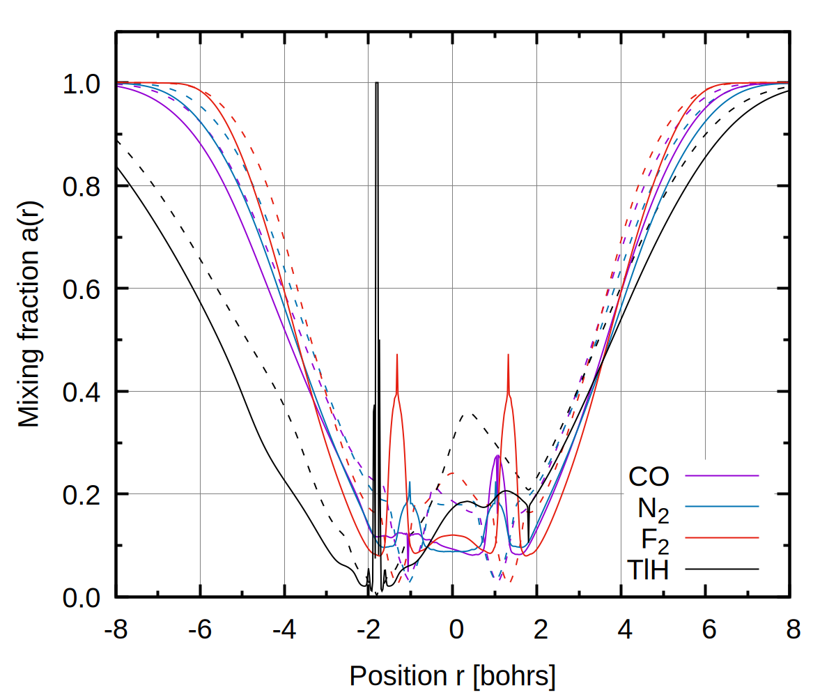
Figure 1: Local mixing function $a$ obtained from TMHF (dashed lines, Ref. 27) and CHYF (solid lines, this work). Properties calculated for four diatomic molecules at self-consistent aug-cc-pVQZ Dunning (1989); Kendall, Dunning, and Harrison (1992); Woon and Dunning (1993) (H, C, N, O, F) and aug-cc-pwCVQZ-DK3 Bross and Peterson (2014) (Tl) orbitals. $a$ is plotted along the internuclear axis. See Supporting Information for complete computational settings.

A plot of the local mixing fraction $a(r)$ is shown in Fig. 1 and compared to the local mixing function of the TMHF functional. The most striking change of new LMF is increases of the amount of exact exchange at the heavy nuclei. In the bonding region, the new LMF leads to a smaller amount of exact exchange. For instance, for N₂ the TMHF LMF leads to about 18% of HF exchange at the center of mass, whereas the new one only leads to approximately 10% of exact exchange being incorporated. In the tail region, the TMHF LMF shows an more rapid increase of $a$ but both LMFs converge to the same limit, i.e. $a\rightarrow 1$.

II.4 Correlation in Local Hybrid Functionals

For a correlation functional that is generally suitable under most circumstances, we again assume the second-order gradient expansion to be detrimental in the slowly varying density limit. To deal with the increased amount of exact exchange in our local hybrid ansatz, yet preserve the second-order gradient expansion of correlation, we suggest the following ansatz:

$$E_{\text{C}}^{\text{SC}}=wE_{\text{C}}^{\text{PBEloc}}+(1-w)E_{\text{C}}^{\text{revPBE}}$$ (32)

and $w$ is the same interpolation function as used in Eq. 21, being suitably flat around $\tau^{\text{vW}}/\tau\approx 0$. The PBEloc correlation is outlined in Ref. 89, while revPBE denotes the revised PBE correlation used in the revTPSS functional. Perdew et al. (2009)

However, both forms remain unsuitable for the limiting iso-orbital case, being unable to yield (nearly) vanishing one electron energies, or obtain the correct correlation energy in the low-density strongly interacting limit. A more suitable form in this limit must be constructed from knowledge of the behavior of electrons in the iso-orbital limit.

1. For a non-degenerate reference, the electron correlation for two-electron systems is approaching a finite limited value. Additionally, correlation energies in physical systems are only weak functions of the density, i.e. correlation in H^-, He, and in the limit of $Z\rightarrow\infty$ are only weakly density dependent.Umrigar and Gonze (1994)

2. In the low density limit of the iso-orbital region, the correlation energy becomes independent of spin polarization.

3. Inter-fermion correlation energies in multicomponent DFT have recently also been shown to only be weakly dependent on the density. Holzer and Franzke (2024)

In addition to these observations, the correlation function should only use occupied KS orbitals throughout for simplicity. Becke (2014)

Following the approach of Becke, we use a coupling strength integration to derive a valid correlation functional. Becke (1988) We propose a coupling strength integrand

$$h^{\alpha\beta}_{\text{C},\lambda}(\vec{r},u)=\frac{2}{\pi}\text{arctan}\left(b_{\text{C}}\tilde{z}_{\alpha\beta}\lambda\right)n_{\beta}\left(u-\tilde{z}_{\alpha\beta}\right)F\left(\gamma_{\alpha\beta}u\right)$$ (33)

with $\gamma_{\alpha\beta}$ being defined as

$$\gamma_{\alpha\beta}= \frac{I_{3}}{\tilde{z}_{\alpha\beta}I_{2}}$$ (34)

$$I_{n}= \int_{0}^{\infty}x^{n}F(x)\textrm{d}x$$ (35)

according to Eqs. (37) and (38) of Ref. 63. $\tilde{z}$ is a scaled version of the correlation length $z^{\text{DME}}$, i.e.

$$\tilde{z}_{\alpha\beta}=c_{\alpha\beta}z_{\alpha\beta}^{\text{DME}}\text{.}$$ (36)

The parameters $b_{\text{C}}$ and $c_{\alpha\beta}$ will be subject to a later optimization. The damping function $F(x)$ is equivalent to the choices presented in Eq. (48) of Ref. 63 and provides a cutoff for the correlation hole when $u$ becomes large. Note that the contribution of the exchange hole vanishes for the opposite-spin case. Hence, $h^{\alpha\beta}_{\text{C},\lambda}(\vec{r},u)=h^{\alpha\beta}_{\lambda}(\vec{r},u)$. Proceeding as outlined by Becke, the potential energy of correlation at a given coupling strength, $U^{\alpha\beta}_{\lambda}$, is obtained as

$$\begin{split}U^{\alpha\beta}_{\lambda}=&\frac{1}{\pi}\int\int\frac{n_{\alpha}(\vec{r})}{u}h^{\alpha\beta}_{\lambda}(\vec{r},u)~{}\textrm{d}u~{}\textrm{d}\vec{r}\\ =&4\frac{I_{2}^{2}}{I_{3}^{3}}\left(I_{2}^{2}-I_{1}I_{3}\right)\int n_{\alpha}n_{\beta}\tilde{z}^{3}_{\alpha\beta}\text{arctan}\left(b_{\text{C}}\tilde{z}_{\alpha\beta}\lambda\right)~{}\textrm{d}\vec{r}\text{.}\end{split}$$ (37)

Subsequently, integration over the coupling strength $\lambda$ is carried out, leading to the final form of the correlation functional in the iso-orbital limit according to

$$\begin{split}E_{\text{C}}^{\alpha\beta,\text{iso}}=&\int_{0}^{1}U^{\alpha\beta}_{\lambda}~{}\textrm{d}\lambda=4\frac{I_{2}^{2}}{I_{3}^{3}}\left(I_{2}^{2}-I_{1}I_{3}\right)\times\\ &\frac{1}{2b_{\text{C}}}\left[\tilde{z}_{\alpha\beta}\text{ln}\left(1+b_{\text{C}}^{2}\tilde{z}_{\alpha\beta}^{2}\right)-2b_{\text{C}}\tilde{z}_{\alpha\beta}^{2}\text{arctan}\left(b_{\text{C}}\tilde{z}_{\alpha\beta}\right)\right]\text{.}\end{split}$$ (38)

The prefactor is evaluated as

$$4\frac{I_{2}^{2}}{I_{3}^{3}}\left(I_{2}^{2}-I_{1}I_{3}\right)\approx 0.5$$ (39)

in a straightforward manner following Ref. 63. It differs from Becke’s suggested values simply by the prefactor of $2\pi^{-1}$ introduced to normalize the arctan function. Eq. 38 provides an interesting result, outlining the correlation energy as a difference between two separate functions. Unlike the original ansatz, Eq. 38 converges to a finite limit in the high density case where $\tilde{z}_{\alpha\beta}\rightarrow 0$. For the same-spin correlation, we have no better guess than the original one of Becke.Becke (1988) The same-spin part is therefore given byBecke (1988)

$$E_{\text{C}}^{\sigma\sigma,\text{iso}}=-0.01\int\rho_{\sigma}D_{\sigma}\tilde{z}^{4}_{\sigma\sigma}\left[1-\frac{2}{z_{\sigma\sigma}}\ln\left(1+\frac{z_{\sigma\sigma}}{2}\right)\right]\textrm{d}\vec{r}\text{,}$$ (40)

with

$$D_{\sigma}=2\left(\tau_{\sigma}-\tau_{\sigma}^{\text{vW}}\right)\text{.}$$ (41)

Here, the factor of two is due to the definition of the kinetic energy density by Becke, which does not include the factor of 1/2, c.f. Eq. 6 in this work and Eq. (31) in Ref. 63. Finally, we realize that in the extreme low-density limit, the correlation energy in the iso-orbital region $E_{\text{C}}^{\text{iso, low}}$ becomes the spin-averaged other-spin correlation energy. To obtain the latter, $\tilde{z}_{\alpha\beta}$ is replaced by

$$\underline{\tilde{z}}=2c_{\alpha\beta}\left(|\underline{U}^{\text{DME}}|^{-1}\right)$$ (42)

with the averaged hole approximation

$$\underline{U}=c_{F}\left[\frac{n}{2}\right]^{1/3}\left(\frac{1}{\underline{f}^{2}}+\frac{7\underline{R}}{9\underline{f}^{4}}\right)\text{.}$$ (43)

Note that for any spin-unpolarized system, $\underline{\tilde{z}}=\tilde{z}$. Subsequently, in the evaluation of the functions $\underline{f}$ and $\underline{R}$, also the spin averaged quantities are used, i.e. $\rho_{\sigma}\rightarrow n/2$. Approximating the correlation length $z$ in an analogous manner to the local mixing function with Eq. 23 from the DME yields the final correlation expression in the iso-orbital limit, i.e.

$$\begin{split}E_{\text{C}}^{\text{iso}}=&w_{\text{C}}(r_{s})E_{\text{C}}^{\text{iso, low}}\\ +&\left[1-w_{\text{C}}(r_{s})\right]\left(E_{\text{C}}^{\alpha\alpha,\text{iso}}+E_{\text{C}}^{\beta\beta,\text{iso}}+E_{\text{C}}^{\alpha\beta,\text{iso}}\right)\text{.}\end{split}$$ (44)

A logistic function $w_{\text{C}}$ based on the local Seitz radius $r_{s}$,

$$w_{\text{C}}(r_{s})=\frac{1}{2}\left[1+\erf\left(\frac{1}{4}\sqrt{\pi}r_{s}-10\right)\right]\text{,}$$ (45)

is used to interpolate between these limits. The smooth interpolation guarantees the low-density limit is approached at $r_{s}>30$ and other correlation parts are turned off. The parameters $b_{\text{C}}=0.112$ and $c_{\alpha\beta}=1.31$ defining the correlation in the iso-orbital limit are finally determined by a least-squares fit to full configuration interaction correlation energies of the same two-electron systems used in Sec. II.3, using the corresponding densities obtained from the optimized local hybrid exchange functional. Note that Eq. 44 is not entirely free of self-correlation errors, as $E_{\text{C}}^{\text{iso, low}}$ will not vanish. However, the largest error is obtained for the hydrogen atom with $5.0\cdot 10^{-6}$ E${}_{\text{h}}$. With the nuclear charge $Z$ growing, it is furthermore quickly diminishing, and for He⁺ and Li²⁺ only a residual error of $4.9\cdot 10^{-7}$ E${}_{\text{h}}$ and $1.6\cdot 10^{-7}$ E${}_{\text{h}}$ is left.

We finally interpolate between the PBE-like correlation energy and the derived iso-orbital energy in an approach similar to Ref. 7 by using the interpolation

$$E_{\text{C}}=f_{C}(\alpha)E_{\text{C}}^{\text{iso}}+\left[1-f_{\text{C}}(\alpha)\right]E_{\text{C}}^{\text{SC}}$$ (46)

where $f_{\text{C}}(\alpha)$ is given by the function

$$f_{\text{C}}(\alpha)=\begin{cases}\alpha<0:e^{-5\alpha/(1-\alpha)}\\ 0<\alpha<1:f_{\text{C},\text{Chebyshev}}(\alpha)\\ \alpha>1:0\end{cases}\text{.}$$ (47)

The Chebyshev polynomials are fit to the function $e^{-5\alpha/(1-\alpha)}$ in the interval $[0,1]$, requiring that $f_{\text{C}}(\alpha=0)=1$ and $f_{\text{C}}(\alpha=1)=0$. A large prefactor of 5 is chosen to make $\partial E_{\text{C}}/\partial\alpha$ sizable near $\alpha\approx 0$ in the low-density, strongly interacting limit. This will lead to a pronounced current-density response in the presence of a magnetic perturbation. The resulting correlation energy, while rather complicated formally, is numerically robust.

The resulting exchange-correlation functional is denoted CHYF general fermions functional in this work.

II.5 Limitations

Herein, dispersion interaction was not considered explicitly. Thus, an extension of the presented model in this direction may be of interest in the future. This could be done either based on the semi-empirical D3 Grimme et al. (2010); Grimme, Ehrlich, and Goerigk (2011) and D4 Caldeweyher et al. (2019) models or based on the parameter-free exchange-hole dipole moment (XDM) dispersion correction. Becke and Johnson (2005, 2007); Otero-de-la Roza and Johnson (2013) The first route was recently followed to obtain the D4 parameters for TMHF and yielded encouraging results. Reimann and Kaupp (2023)

As a further limitation, the ansatz presented herein is not intended for systems with strong correlation, i.e. systems with large mixing of configurations. As shown in the B13 functional, Becke (2013) these systems require an additional term for the strong-correlation contribution.

Finally, we note that the seminumerical implementations of LHFs (see next subsection) are restricted to finite systems and periodic systems are therefore beyond the scope of the present work.

II.6 Implementation

The new functional described herein is implemented in TURBOMOLE Ahlrichs et al. (1989); Balasubramani et al. (2020); Franzke et al. (2023); TURBOMOLE GmbH (2023) based on the given MAPLE files. The functional designed in this work does not include a calibration function and only includes the density, its gradient, and the kinetic energy density. The latter is generalized with the current density for magnetic properties, excited states, and spin–orbit coupling as noted above. Therefore, the new functional is directly available for the electronic ground-state self-consistent field (SCF) formalism and the related expectation values, Bahmann and Kaupp (2015); Holzer (2020) analytical geometry gradients, Klawohn, Bahmann, and Kaupp (2016) excitation energies Maier, Bahmann, and Kaupp (2015); Holzer (2020); Kehry et al. (2020) and excited-state geometries Grotjahn, Furche, and Kaupp (2019) from time-dependent density functional theory (TDDFT) as well as quasiparticle states from the Green’s function $GW$ formalism, Holzer, Franzke, and Kehry (2021) nuclear magnetic resonance (NMR) parameters Schattenberg et al. (2020); Schattenberg and Kaupp (2021); Franzke, Mack, and Weigend (2021); Gillhuber, Franzke, and Weigend (2021); Franzke et al. (2024) and electron paramagnetic resonance (EPR) properties. Franzke and Holzer (2022); Bruder, Franzke, and Weigend (2022); Bruder et al. (2023); Franzke et al. (2024); Franzke and Yu (2022a, b) The self-consistent two-component formalism is available for the SCF energies, EPR properties, NMR coupling constants, TDDFT excitation energies, polarizabilities, and the $GW$ formalism. Wodyński and Kaupp (2020); Holzer (2020); Holzer, Franzke, and Pausch (2022); Franzke, Mack, and Weigend (2021); Kehry et al. (2020); Holzer and Klopper (2019); Holzer (2023) Two-component NMR shieldings and EPR g-tensors can only be calculated with a common gauge origin. Holzer, Franzke, and Pausch (2022); Franzke and Holzer (2023) Furthermore, the evaluation of Mössbauer contact densities is implemented in the present work, see the Supporting Information. Special relativity is either introduced with effective core potentials Armbruster et al. (2008); Baldes and Weigend (2013) or all-electron approaches such as exact two-component (X2C) theory. Peng et al. (2013); Franzke, Middendorf, and Weigend (2018)

III Computational Methods

The accuracy of the new density functional approximation is assessed for thermochemical properties such as atomization energies and barrier heights, excitation energies, Mössbauer isomer shifts, NMR spin–spin coupling constants, NMR shieldings and shifts, magnetizabilities, EPR hyperfine coupling constants, and EPR g-tensors. Here, NMR coupling constants, NMR shifts, and EPR properties are also calculated within the relativistic framework, which is necessary for heavy elements.

For brevity, computational details for the benchmark studies below are listed in the Supporting Information. Furthermore, results for Mössbauer isomer shifts or contact densities, NMR coupling constants, NMR shielding constants and shifts, as well as EPR hyperfine coupling constants and EPR g-tensors are only presented in the Supporting Information. Here, we just stress the main findings from these benchmark studies. That is, the new LHF improves the performance for Mössbauer isomer shifts and NMR shieldings. NMR shieldings and shifts were among the properties described poorly by the predecessor TMHF. EPR properties are still obtained with good accuracy. Therefore, the new functional eliminates the main weakness of TMHF and is consequently more general and robust.

IV Results and Discussion

IV.1 Thermochemistry and Electronic Ground State

For the thermochemical W4-11 test set, Karton, Daon, and Martin (2011) being composed of 140 atomization energies, the new local hybrid functional is able to outperform other functionals that have been designed with theoretically constrained satisfaction in mind. As shown in Fig. 2, CHYF manages to be at least on par with common functionals such as PBE0, Perdew, Burke, and Ernzerhof (1996); Adamo and Barone (1999) TPSSh, Tao et al. (2003); Staroverov et al. (2003) and SCAN, Sun, Ruzsinszky, and Perdew (2015) with the latter yielding stellar performance for a pure meta-GGA functional.

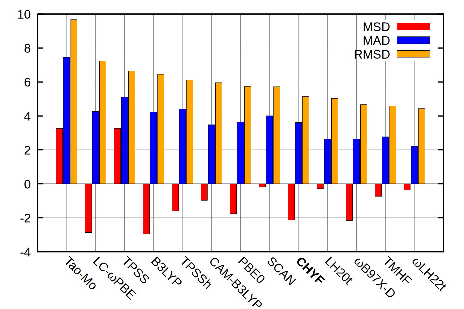
Figure 2: Mean standard deviation (MSD), mean average deviation (MAD), and root mean square deviation (RMSD) for the atomization energies of the W4-11 test set. All values are in kcal/mol.

Even though we have carefully adapted of the correlation energy term in Sec. II.4, CHYF still has a pronounced tendency of underbinding in molecular systems. Root mean square deviations are, however, comparable to thermochemically optimized local hybrids such as LH20t, Haasler et al. (2020) and only slightly worse than those of the thermochemically optimized range-separated (local) hybrids B97X-D Chai and Head-Gordon (2008) and LH22t. Fürst and Kaupp (2023)

For barrier heights, tested with the BH76 test set, Zhao, González-García, and Truhlar (2005); Zhao, Lynch, and Truhlar (2005); Goerigk and Grimme (2010) CHYF exhibits an interesting behavior. It generally behaves like a pure density functional, with the mean absolute deviation (MAD) being roughly the negative mean signed deviation (MSD). This indicates generally too low barrier heights. Contrary to hybrid functionals such as, for example, PBE0 Perdew, Burke, and Ernzerhof (1996); Adamo and Barone (1999) or B3LYP, Lee, Yang, and Parr (1988); Becke (1993); Stephens et al. (1994) which no longer show the same relation for MSD and MAD, still a lower RMSD value is obtained. This outlines that our proposed functional at its core is more related to pure density functionals than it is to hybrid functionals. Yet, still viable improvements over other functionals that have not been thermochemically optimized are observed. The thermochemically optimized local and range-separated hybrid functionals yield significantly lower deviations for the BH76 test set, as does the TMHF functional.

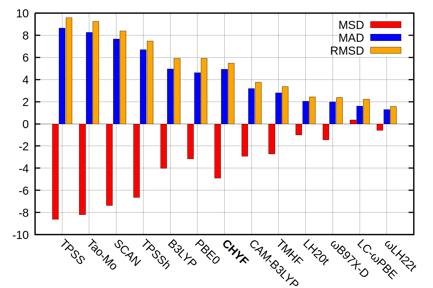
Figure 3: Mean standard deviation (MSD), mean absolute deviation (MAD), and root mean square deviation (RMSD) for the barrier heights of the BH76 test set. All values are in kcal/mol.

Overall, we deem this accuracy for thermochemistry to be sufficient for a general and transferable local hybrid, that favors a first-principles-based construction over thermochemical optimization.

IV.2 Numerical Behavior and Stability

The numerical requirements of CHYF are further comparably low. As outlined by Table 1, the grid dependence of the functional is less pronounced than one may suspect from the complicated structure arising in Sec. II. Already very small grids provide sufficiently accurate results, both in terms of relative and absolute deviations. Already with the smallest grid 1, Treutler (1995); Treutler and Ahlrichs (1995) results that are sufficiently converged for most purposes are obtained. Total energies are already accurate to $10^{-3}$ a.u., which subsequently improves smoothly with increasing grid sizes.

Table 1: Grid dependence of CHYF for the W4-11 test set of atomization energies. Mean absolute energy differences between total energies $\Delta\bar{E}$ are given with respect to grid 7. Treutler (1995); Treutler and Ahlrichs (1995)

Grid	MSD	MAD	RMSD	$\Delta\bar{E}$
	[kcal/mol]	[kcal/mol]	[kcal/mol]	[a.u.]
7	$-2.148$	$3.614$	$5.161$	–
6	$-2.145$	$3.613$	$5.140$	$5.93\cdot 10^{-6}$
5	$-2.142$	$3.612$	$5.140$	$1.37\cdot 10^{-5}$
4	$-2.136$	$3.608$	$5.136$	$1.63\cdot 10^{-5}$
3	$-2.135$	$3.608$	$5.138$	$2.08\cdot 10^{-4}$
2	$-2.122$	$3.614$	$5.141$	$4.92\cdot 10^{-4}$
1	$-2.124$	$3.586$	$5.110$	$1.17\cdot 10^{-3}$

Due to the high numerical stability, also no issues regarding the convergence of the SCF iterations were observed in any calculation performed in this work. While certainly more subjective than the results in Table 1, we find that convergence is generally very smooth, with even problematic cases as, e.g., relativistic two-component open-shell complexes converging very well in this work.

Overall, the computational demands associated with local hybrid functionals are substantially reduced by this grid behavior. This allows to use small grids for calculations without loss of accuracy. This is especially advantageous for the exact exchange terms, which can become a computational overhead for the seminumerical evaluation of LHFs compared to the corresponding multigrid approach for global or range-separated hybrids. Neese et al. (2009); Plessow and Weigend (2012); Holzer (2020); Stoychev et al. (2018); Holzer, Franzke, and Kehry (2021); Helmich-Paris et al. (2021) The latter uses a larger grid for the semilocal DFT exchange than for the exact exchange terms. Especially for response calculations, very small grids are usually sufficient for the latter. Holzer (2020); Holzer, Franzke, and Kehry (2021); Bruder et al. (2023); Franzke and Holzer (2023) Therefore, we expect CHYF to be competitive to PBE0 in terms of computational costs for “real-world” quantum chemical studies.

IV.3 Electronic Excitation Energies with TDDFT

The excited state test set of Ref. 128 is remarkable in one respect: It compiles a set of high-quality experimental references, ab initio data, and accounts for geometrical changes during the excitation, as well as zero-point vibrational energy contributions. To perform well in this test, a method must therefore be able to describe ground and excited states reasonably well.

As outlined by the results in Table 2, this is a substantial task for density functional approximations. Especially the root-mean-square deviation (RMSD) reveals that a barrier exists at 0.3 eV. And this barrier cannot easily be overcome by climbing the functional ladder, as revealed by the stagnating errors when going from (meta-)GGAs to hybrid or even local hybrid functionals, where the RMSD is often significantly worsened when compared to their parent functional. Also recent local hybrid functionals obtained by extensive fitting procedures as LH20tHaasler et al. (2020) and and the range-separated local hybrid LH22tFürst and Kaupp (2023) are unable to rectify this. Instead, they invert the general trend of underestimating excited state energies, but no further changes of the magnitude of errors is observed.

Table 2: Mean signed deviation (MSD), mean absolute deviation (MAD), root mean square deviation (RMSD), and maximum deviation (Max.) for 41 excited states of 37 molecules compared to experimental data as outlined in Ref. 128. Values for other functionals are taken from Ref. 27 and Ref. 128. All values are in eV.

	MSD	MAD	RMSD	Max.
PBE	$-0.204$	$0.240$	$0.301$	$0.632$
TPSS	$-0.169$	$0.230$	$0.287$	$0.655$
B3LYP	$-0.192$	$0.265$	$0.355$	$0.828$
PBE0	$-0.138$	$0.273$	$0.333$	$0.734$
TPSSh	$-0.119$	$0.237$	$0.318$	$0.774$
CAM-B3LYP	$-0.100$	$0.274$	$0.338$	$0.709$
LC-PBE	$-0.021$	$0.291$	$0.311$	$0.588$
B97X-D	$-0.097$	$0.273$	$0.333$	$0.693$
LH20t	$0.121$	$0.258$	$0.313$	$0.658$
LH22t	$0.100$	$0.267$	$0.313$	$0.619$
TMHF	$0.002$	$0.246$	$0.276$	$0.467$
CHYF	$0.005$	$0.230$	$0.264$	$0.508$
CC2	$0.045$	$0.083$	$0.112$	$0.270$
CCSD	$0.177$	$0.177$	$0.204$	$0.429$
ADC(3)	$-0.125$	$0.228$	$0.271$	$0.488$
CC3	$-0.011$	$0.025$	$0.036$	$0.107$

By using a construction based on first principles, as outlined in this work and previously for TMHF—albeit only for exchange in the latter case—this barrier can be overcome. Both TMHF and CHYF cut the RMSD by approximately 20 % compared to other density functional approximations, while also significantly cutting down on the maximum error observed. The overall balanced description of excited states is further emphasized by the mean signed deviation approaching zero for both methods. For these functionals, the accuracy levels provided by density functional theory are within the grasp of high-level methods such as CCSD for the first time. An odd pick of wavefunction-based methods, as for example ADC(3), could even leave one with no advantage over TMHF or CHYF. We, however, admit that ADC(3) is a notoriously bad pick for excited states,Suellen et al. (2019) and should never be used over CC3 at the same $\mathcal{O}(N^{7})$ computational cost. Nevertheless, ADC(3) serves as warning that a simple assumption of wavefunction-based methods outperforming density functional theory based ones for excited states has become obsolete.

V Conclusion

In this work, we have derived a local hybrid functional from theoretical constraints, only taking one- and two-electron systems into account for exchange and correlation. Augmenting these with the known gradient expansions of the uniform electron gas results in the CHYF functional. The latter is the first local hybrid functional that is fully compatible with a correlation functional that follows the second-order gradient expansion, yet does incorporate large amounts of exact exchange. CHYF generally exhibits a behavior that resembles an optimal pure density functionals in many respects concerning thermochemical properties. Yet, it is strikingly different in its ability to predict higher-order properties, as for example excited states. For the latter, it is shown that a very accurate description of the excited states can be obtained, significantly outperforming any other density functional. Further investigations of various properties also outline that our newly developed functional is robust, leading to clearly acceptable results for all tested cases. This is a unique feature in density functional theory, and can trigger further developments in the direction of virtually parameter-free density functionals.

Supplementary Material

Results for Mössbauer isomer shifts, NMR and EPR properties are presented (Supporting-Information.pdf). Spreadsheets with all results are available (W4-11.xlsx, BH76.xlsx, TDDFT.xlsx, Magnetizabilities.xlsx, Mossbauer.xlsx, NMR-Couplings.xlsx, Sn-NMR-Couplings.xlsx, NMR-Shieldings.xlsx, NMR-Shifts.xlsx, 17O-NMR-Shifts.xlsx, EPR.xlsx, EPR-2c.xlsx, E-P-Correlation.xlsx). Molecular structures optimized in this work are given in txt files (Structures-NMR-Couplings.txt and Structures-NMR-Shifts.txt). The uncontracted augmented Dyall-CVTZ basis set (aug-Dyall-CVTZ.txt) is further included. All of these files are collected in the archive Data.zip. Maple files of the new functional are provided.

Author Declarations

Conflict of Interest

The authors have no conflicts to disclose.

Author Contributions

Christof Holzer: Conceptualization (lead); Data curation (equal); Formal analysis (equal); Investigation (equal); Methodology (lead); Software (equal); Validation (equal); Visualization (equal); Writing – original draft (equal); Writing – review & editing (equal).
Yannick J. Franzke: Conceptualization (supporting); Data curation (equal); Formal analysis (equal); Investigation (equal); Methodology (supporting); Software (equal); Validation (equal); Visualization (equal); Writing – original draft (equal); Writing – review & editing (equal).

Data Availability Statement

The data that support the findings of this study are available within the article and its supplementary material.

Appendix A Extension Towards Multicomponent Density Functional Theory

Notably, DFT is not restricted to electrons but can be extended to a many-fermion version, termed multicomponent DFT (MC-DFT). Kreibich and Gross (2001); van Leeuwen and Gross (2006); Chakraborty, Pak, and Hammes-Schiffer (2008); Kreibich, van Leeuwen, and Gross (2008) Most commonly, MC-DFT is used with protons, as the respective MC-DFT approach, termed nuclear electronic orbital (NEO), goes beyond the established Born–Oppenheimer approximation. Messud (2011); Brorsen, Yang, and Hammes-Schiffer (2017); Yu and Hammes-Schiffer (2020); Pavošević, Culpitt, and Hammes-Schiffer (2020); Hammes-Schiffer (2021) Just like the common electronic DFT framework, MC-DFT also relies on accurate density functional approximations. In the last two decades, electron-proton Udagawa, Tsuneda, and Tachikawa (2014); Pak, Chakraborty, and Hammes-Schiffer (2007); Chakraborty, Pak, and Hammes-Schiffer (2008, 2009); Sirjoosingh, Pak, and Hammes-Schiffer (2011, 2012); Yang et al. (2017); Brorsen, Schneider, and Hammes-Schiffer (2018); Tao, Yang, and Hammes-Schiffer (2019) and electron-muon correlation functionals Goli and Shahbazian (2022); Deng et al. (2023) were developed and successfully applied. Ideally, a general density functional approximations applicable to electrons, protons, and other fermions with similar accuracy should be constructed.

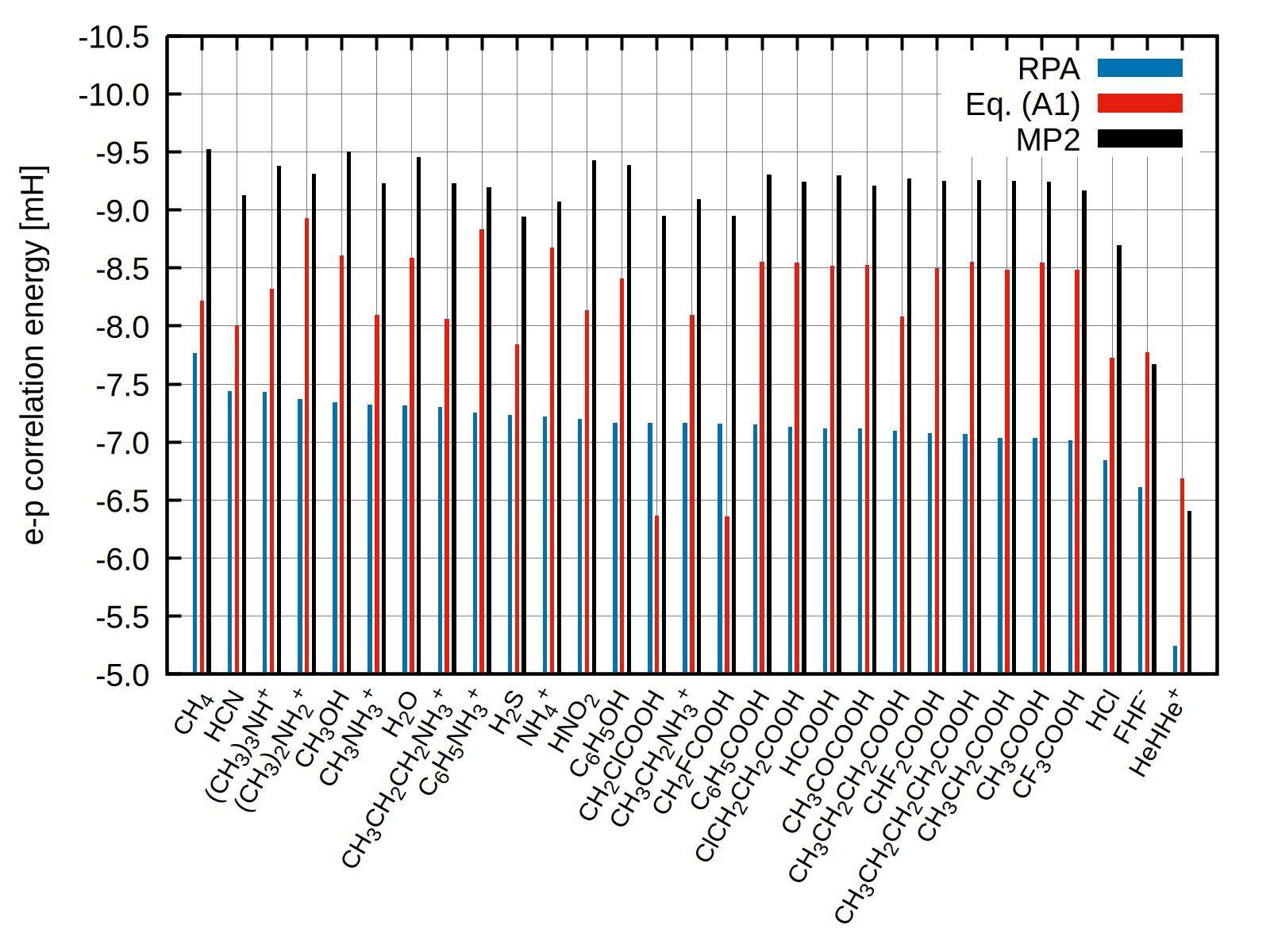
Figure 4: Electron-proton correlation energies for 29 molecular systems obtained at the RPA@TMHF, Eq. 48@TMHF+epc17-1, and MP2@HF level of theory. epc17-1 refers to the electron-proton correlation functional of Ref. 143. All values are in atomic units (milli-Hartree).

To underline the generality and transferability of our ansatz, we note that Eq. 38 can be modified to be compatible with general inter-fermion correlation. Assuming that the inter-fermion correlation is solely dependent on the total density, the electron-electron correlation length is replaced with the appropriate electron-fermion correlation length

$$\underline{z}^{\text{DME}}_{ep}= \left(|\underline{U}_{e}^{\text{DME}}|^{-1}+|\underline{U}_{p}^{\text{DME}}|^{-1}\right)\text{.}$$ (48)

Only the parameters to determine $\underline{U}_{p}^{\text{DME}}$ are additionally required. We go forward by shortly demonstrating this for protons. Naively assuming that $\beta=79.873$ is serviceable also for protons, we re-optimizing $\lambda=0.5922$ by fitting this value to the hydrogen atom. During the fitting procedure, both electron and proton are being treated as quantum particles. Note that $E_{\text{C}}^{\text{SC}}$ is not needed for the electron-proton correlation.

Comparing electron-proton correlation energies from this ansatz with recently evaluated correlation energies Holzer and Franzke (2024) from the random phase approximation (RPA) (and second-order Møller–Plesset perturbation theory (MP2) reveals that Eq. 48 indeed delivers reasonable electron-proton correlation energies. Computational settings are the same as in Ref. 20. Eq. 48 is evaluated non-selfconsistently at the respective TMHF+epc17-1 densities.

As outlined by Fig. 4, the electron-proton correlation energies predicted by Eq. 48 are between those obtained from the RPA and those from MP2. The anomaly at HeHHe⁺, which exhibits an exceptionally low electron-proton correlation energy is well recovered. Also, FHF^- is correctly predicted to again have a comparably low electron-proton correlation. Deficiencies can be seen for the halogenated acetic acid derivatives, where Eq. 48 yields comparably low correlation energies, while both RPA and MP2 do not find anomalies for these molecules. The differences are not too high though, and especially involving halogen atoms could lead to more pronounced effects of the neglected self-consistency in the electron-proton correlation, or hinting at our quick re-optimization of the parameters $\lambda$ and $\beta$ being insufficient. While certainly a full reoptimization of all parameters for the proton would be necessary to yield optimal results, we emphasize that the proof of concept of a single density functional being valid for various different fermions has been very successful. This is an even more remarkable result when considering that the local hybrid functional was derived from first principles by satisfying theoretical constraints.

References

References

- Csonka, Perdew, and Ruzsinszky (2010) G. I. Csonka, J. P. Perdew, and A. Ruzsinszky, J. Chem. Theory Comput. 6, 3688 (2010).
- Burke (2012) K. Burke, J. Chem. Phys. 136, 150901 (2012).
- Becke (2014) A. D. Becke, J. Chem. Phys. 140, 18A301 (2014).
- Mardirossian and Head-Gordon (2017) N. Mardirossian and M. Head-Gordon, Mol. Phys. 115, 2315 (2017).
- Perdew and Schmidt (2001) J. P. Perdew and K. Schmidt, AIP Conf. Proc. 577, 1 (2001).
- Tao and Mo (2016) J. Tao and Y. Mo, Phys. Rev. Lett. 117, 073001 (2016).
- Sun, Ruzsinszky, and Perdew (2015) J. Sun, A. Ruzsinszky, and J. P. Perdew, Phys. Rev. Lett. 115, 036402 (2015).
- Furness et al. (2020a) J. W. Furness, A. D. Kaplan, J. Ning, J. P. Perdew, and J. Sun, J. Phys. Chem. Lett. 11, 8208 (2020a).
- Furness et al. (2020b) J. W. Furness, A. D. Kaplan, J. Ning, J. P. Perdew, and J. Sun, J. Phys. Chem. Lett. 11, 9248 (2020b).
- Medvedev et al. (2017) M. G. Medvedev, I. S. Bushmarinov, J. Sun, J. P. Perdew, and K. A. Lyssenko, Science 355, 49 (2017).
- Becke (2022a) A. D. Becke, J. Chem. Phys. 156, 214101 (2022a).
- Becke (2022b) A. D. Becke, J. Chem. Phys. 157, 234102 (2022b).
- Jaramillo, Scuseria, and Ernzerhof (2003) J. Jaramillo, G. E. Scuseria, and M. Ernzerhof, J. Chem. Phys. 118, 1068 (2003).
- Becke (1993) A. D. Becke, J. Chem. Phys. 98, 5648 (1993).
- Stephens et al. (1994) P. J. Stephens, F. J. Devlin, C. F. Chabalowski, and M. J. Frisch, J. Phys. Chem. 98, 11623 (1994).
- Gill, Adamson, and Pople (1996) P. W. Gill, R. D. Adamson, and J. A. Pople, Mol. Phys. 88, 1005 (1996).
- Leininger et al. (1997) T. Leininger, H. Stoll, H.-J. Werner, and A. Savin, Chem. Phys. Lett. 275, 151 (1997).
- Iikura et al. (2001) H. Iikura, T. Tsuneda, T. Yanai, and K. Hirao, J. Chem. Phys. 115, 3540 (2001).
- Yanai, Tew, and Handy (2004) T. Yanai, D. P. Tew, and N. C. Handy, Chem. Phys. Lett. 393, 51 (2004).
- Holzer and Franzke (2024) C. Holzer and Y. J. Franzke, ChemPhysChem 25, e202400120 (2024).
- Johnson (2014) E. R. Johnson, J. Chem. Phys. 141, 124120 (2014).
- Schmidt et al. (2014) T. Schmidt, E. Kraisler, A. Makmal, L. Kronik, and S. Kümmel, J. Chem. Phys. 140, 18A510 (2014).
- Arbuznikov and Kaupp (2007) A. V. Arbuznikov and M. Kaupp, Chem. Phys. Lett. 440, 160 (2007).
- Arbuznikov and Kaupp (2014) A. V. Arbuznikov and M. Kaupp, J. Chem. Phys. 141, 204101 (2014).
- Haasler et al. (2020) M. Haasler, T. M. Maier, R. Grotjahn, S. Gückel, A. V. Arbuznikov, and M. Kaupp, J. Chem. Theory Comput. 16, 5645 (2020).
- Tao et al. (2008) J. Tao, V. N. Staroverov, G. E. Scuseria, and J. P. Perdew, Phys. Rev. A 77, 012509 (2008).
- Holzer and Franzke (2022) C. Holzer and Y. J. Franzke, J. Chem. Phys. 157, 034108 (2022).
- de Silva and Corminboeuf (2015) P. de Silva and C. Corminboeuf, J. Chem. Phys. 142, 074112 (2015).
- Janesko and Scuseria (2007) B. G. Janesko and G. E. Scuseria, J. Chem. Phys. 127, 164117 (2007).
- Janesko, Krukau, and Scuseria (2008) B. G. Janesko, A. V. Krukau, and G. E. Scuseria, J. Chem. Phys. 129, 124110 (2008).
- Janesko and Scuseria (2008) B. G. Janesko and G. E. Scuseria, J. Chem. Phys. 128, 084111 (2008).
- Maier, Arbuznikov, and Kaupp (2019) T. M. Maier, A. V. Arbuznikov, and M. Kaupp, Wiley Interdiscip. Rev.: Comput. Mol. Sci. 9, e1378 (2019).
- Janesko (2021) B. G. Janesko, Chem. Soc. Rev. 50, 8470 (2021).
- Grotjahn (2023) R. Grotjahn, J. Chem. Phys. 159, 174102 (2023).
- Plessow and Weigend (2012) P. Plessow and F. Weigend, J. Comput. Chem. 33, 810 (2012).
- Laqua, Kussmann, and Ochsenfeld (2018) H. Laqua, J. Kussmann, and C. Ochsenfeld, J. Chem. Theory Comput. 14, 3451 (2018).
- Klawohn, Bahmann, and Kaupp (2016) S. Klawohn, H. Bahmann, and M. Kaupp, J. Chem. Theory Comput. 12, 4254 (2016).
- Holzer, Franzke, and Kehry (2021) C. Holzer, Y. J. Franzke, and M. Kehry, J. Chem. Theory Comput. 17, 2928 (2021).
- Jiménez-Hoyos et al. (2009) C. A. Jiménez-Hoyos, B. G. Janesko, G. E. Scuseria, V. N. Staroverov, and J. P. Perdew, Mol. Phys. 107, 1077 (2009).
- Liu et al. (2012) F. Liu, E. Proynov, J.-G. Yu, T. R. Furlani, and J. Kong, J. Chem. Phys. 137, 114104 (2012).
- Maier, Bahmann, and Kaupp (2015) T. M. Maier, H. Bahmann, and M. Kaupp, J. Chem. Theory Comput. 11, 4226 (2015).
- Grotjahn, Furche, and Kaupp (2019) R. Grotjahn, F. Furche, and M. Kaupp, J. Chem. Theory Comput. 15, 5508 (2019).
- Kehry et al. (2020) M. Kehry, Y. J. Franzke, C. Holzer, and W. Klopper, Mol. Phys. 118, e1755064 (2020).
- Holzer (2020) C. Holzer, J. Chem. Phys. 153, 184115 (2020).
- Zerulla et al. (2022) B. Zerulla, M. Krstić, D. Beutel, C. Holzer, C. Wöll, C. Rockstuhl, and I. Fernandez-Corbaton, Adv. Mater. 34, 2200350 (2022).
- Zerulla et al. (2023a) B. Zerulla, R. Venkitakrishnan, D. Beutel, M. Krstić, C. Holzer, C. Rockstuhl, and I. Fernandez-Corbaton, Adv. Opt. Mater. 11, 2201564 (2023a).
- Zerulla et al. (2023b) B. Zerulla, C. Li, D. Beutel, S. Oßwald, C. Holzer, J. Bürck, S. Bräse, C. Wöll, I. Fernandez-Corbaton, L. Heinke, C. Rockstuhl, and M. Krstić, Adv. Funct. Mater. 34, 2301093 (2023b).
- Müller et al. (2022) M. M. Müller, N. Perdana, C. Rockstuhl, and C. Holzer, J. Chem. Phys. 156, 094103 (2022).
- Rai et al. (2023a) V. Rai, N. Balzer, G. Derenbach, C. Holzer, M. Mayor, W. Wulfhekel, L. Gerhard, and M. Valášek, Nat Commun. 14, 8253 (2023a).
- Rai et al. (2023b) V. Rai, L. Gerhard, N. Balzer, M. Valášek, C. Holzer, L. Yang, M. Wegener, C. Rockstuhl, M. Mayor, and W. Wulfhekel, Phys. Rev. Lett. 130, 036201 (2023b).
- Schattenberg et al. (2020) C. J. Schattenberg, K. Reiter, F. Weigend, and M. Kaupp, J. Chem. Theory Comput. 16, 931 (2020).
- Mack et al. (2020) F. Mack, C. J. Schattenberg, M. Kaupp, and F. Weigend, J. Phys. Chem. A 124, 8529 (2020).
- Franzke, Mack, and Weigend (2021) Y. J. Franzke, F. Mack, and F. Weigend, J. Chem. Theory Comput. 17, 3974 (2021).
- Franzke and Holzer (2022) Y. J. Franzke and C. Holzer, J. Chem. Phys. 157, 031102 (2022).
- Holzer, Franzke, and Pausch (2022) C. Holzer, Y. J. Franzke, and A. Pausch, J. Chem. Phys. 157, 204102 (2022).
- Bruder, Franzke, and Weigend (2022) F. Bruder, Y. J. Franzke, and F. Weigend, J. Phys. Chem. A 126, 5050 (2022).
- Franzke (2023) Y. J. Franzke, J. Chem. Theory Comput. 19, 2010 (2023).
- Bruder et al. (2023) F. Bruder, Y. J. Franzke, C. Holzer, and F. Weigend, J. Chem. Phys. 159, 194117 (2023).
- Franzke et al. (2024) Y. J. Franzke, F. Bruder, S. Gillhuber, C. Holzer, and F. Weigend, J. Phys. Chem. A 128, 670 (2024).
- Vosko, Wilk, and Nusair (1980) S. H. Vosko, L. Wilk, and M. Nusair, Can. J. Phys. 58, 1200 (1980).
- Perdew, Burke, and Ernzerhof (1996) J. P. Perdew, K. Burke, and M. Ernzerhof, Phys. Rev. Lett. 77, 3865 (1996).
- Perdew and Wang (1992) J. P. Perdew and Y. Wang, Phys. Rev. B 45, 13244 (1992).
- Becke (1988) A. D. Becke, J. Chem. Phys. 88, 1053 (1988).
- Becke (1996) A. D. Becke, J. Chem. Phys. 104, 1040 (1996).
- Arbuznikov and Kaupp (2012) A. V. Arbuznikov and M. Kaupp, J. Chem. Phys. 136, 014111 (2012).
- Dobson (1993) J. F. Dobson, J. Chem. Phys. 98, 8870 (1993).
- Becke (2002) A. D. Becke, J. Chem. Phys. 117, 6935 (2002).
- Tao (2005) J. Tao, Phys. Rev. B 71, 205107 (2005).
- Bates and Furche (2012) J. E. Bates and F. Furche, J. Chem. Phys. 137, 164105 (2012).
- Grotjahn, Furche, and Kaupp (2022) R. Grotjahn, F. Furche, and M. Kaupp, J. Chem. Phys. 157, 111102 (2022).
- Grotjahn and Furche (2023) R. Grotjahn and F. Furche, J. Chem. Theory Comput. 19, 4897 (2023).
- Schattenberg and Kaupp (2021) C. J. Schattenberg and M. Kaupp, J. Chem. Theory Comput. 17, 1469 (2021).
- Pausch and Holzer (2022) A. Pausch and C. Holzer, J. Phys. Chem. Lett. 13, 4335 (2022).
- Franzke and Holzer (2024) Y. J. Franzke and C. Holzer, J. Chem. Phys. 160, 184101 (2024).
- Cruz, Lam, and Burke (1998) F. G. Cruz, K.-C. Lam, and K. Burke, J. Phys. Chem. A 102, 4911 (1998).
- Burke, Cruz, and Lam (1998) K. Burke, F. G. Cruz, and K.-C. Lam, J. Chem. Phys. 109, 8161 (1998).
- Maier et al. (2016) T. M. Maier, M. Haasler, A. V. Arbuznikov, and M. Kaupp, Phys. Chem. Chem. Phys. 18, 21133 (2016).
- Brack, Jennings, and Chu (1976) M. Brack, B. Jennings, and Y. Chu, Phys. Lett. 65B, 1 (1976).
- Perdew et al. (1999) J. P. Perdew, S. Kurth, A. c. v. Zupan, and P. Blaha, Phys. Rev. Lett. 82, 2544 (1999).
- Wang and Perdew (1991) Y. Wang and J. P. Perdew, Phys. Rev. B 43, 8911 (1991).
- Perdew, Burke, and Wang (1996) J. P. Perdew, K. Burke, and Y. Wang, Phys. Rev. B 54, 16533 (1996).
- Perdew et al. (2009) J. P. Perdew, A. Ruzsinszky, G. I. Csonka, L. A. Constantin, and J. Sun, Phys. Rev. Lett. 103, 026403 (2009).
- Umrigar and Gonze (1994) C. J. Umrigar and X. Gonze, Phys. Rev. A 50, 3827 (1994).
- Tao et al. (2003) J. Tao, J. P. Perdew, V. N. Staroverov, and G. E. Scuseria, Phys. Rev. Lett. 91, 146401 (2003).
- Dunning (1989) T. H. Dunning, J. Chem. Phys. 90, 1007 (1989).
- Kendall, Dunning, and Harrison (1992) R. A. Kendall, T. H. Dunning, and R. J. Harrison, J. Chem. Phys. 96, 6796 (1992).
- Woon and Dunning (1993) D. E. Woon and T. H. Dunning, J. Chem. Phys. 98, 1358 (1993).
- Bross and Peterson (2014) D. H. Bross and K. A. Peterson, Theor. Chem. Acc. 133, 1434 (2014).
- Constantin, Fabiano, and Sala (2012) L. A. Constantin, E. Fabiano, and F. D. Sala, Phys. Rev. B 86, 035130 (2012).
- Grimme et al. (2010) S. Grimme, J. Antony, S. Ehrlich, and H. Krieg, J. Chem. Phys. 132, 154104 (2010).
- Grimme, Ehrlich, and Goerigk (2011) S. Grimme, S. Ehrlich, and L. Goerigk, J. Comput. Chem. 32, 1456 (2011).
- Caldeweyher et al. (2019) E. Caldeweyher, S. Ehlert, A. Hansen, H. Neugebauer, S. Spicher, C. Bannwarth, and S. Grimme, J. Chem. Phys. 150, 154122 (2019).
- Becke and Johnson (2005) A. D. Becke and E. R. Johnson, J. Chem. Phys. 123, 154101 (2005).
- Becke and Johnson (2007) A. D. Becke and E. R. Johnson, J. Chem. Phys. 127, 154108 (2007).
- Otero-de-la Roza and Johnson (2013) A. Otero-de-la Roza and E. R. Johnson, J. Chem. Phys. 138, 204109 (2013).
- Reimann and Kaupp (2023) M. Reimann and M. Kaupp, J. Chem. Theory Comput. 19, 97 (2023).
- Becke (2013) A. D. Becke, J. Chem. Phys. 138, 074109 (2013).
- Ahlrichs et al. (1989) R. Ahlrichs, M. Bär, M. Häser, H. Horn, and C. Kölmel, Chem. Phys. Lett. 162, 165 (1989).
- Balasubramani et al. (2020) S. G. Balasubramani, G. P. Chen, S. Coriani, M. Diedenhofen, M. S. Frank, Y. J. Franzke, F. Furche, R. Grotjahn, M. E. Harding, C. Hättig, A. Hellweg, B. Helmich-Paris, C. Holzer, U. Huniar, M. Kaupp, A. Marefat Khah, S. Karbalaei Khani, T. Müller, F. Mack, B. D. Nguyen, S. M. Parker, E. Perlt, D. Rappoport, K. Reiter, S. Roy, M. Rückert, G. Schmitz, M. Sierka, E. Tapavicza, D. P. Tew, C. van Wüllen, V. K. Voora, F. Weigend, A. Wodyński, and J. M. Yu, J. Chem. Phys. 152, 184107 (2020).
- Franzke et al. (2023) Y. J. Franzke, C. Holzer, J. H. Andersen, T. Begušić, F. Bruder, S. Coriani, F. Della Sala, E. Fabiano, D. A. Fedotov, S. Fürst, S. Gillhuber, R. Grotjahn, M. Kaupp, M. Kehry, M. Krstić, F. Mack, S. Majumdar, B. D. Nguyen, S. M. Parker, F. Pauly, A. Pausch, E. Perlt, G. S. Phun, A. Rajabi, D. Rappoport, B. Samal, T. Schrader, M. Sharma, E. Tapavicza, R. S. Treß, V. Voora, A. Wodyński, J. M. Yu, B. Zerulla, F. Furche, C. Hättig, M. Sierka, D. P. Tew, and F. Weigend, J. Chem. Theory Comput. 19, 6859 (2023).
- TURBOMOLE GmbH (2023) TURBOMOLE GmbH, (2023), developers’ version of TURBOMOLE V7.8.1, a development of University of Karlsruhe and Forschungszentrum Karlsruhe GmbH, 1989-2007, TURBOMOLE GmbH, since 2007; available from https://www.turbomole.org (retrieved March 4, 2024).
- Bahmann and Kaupp (2015) H. Bahmann and M. Kaupp, J. Chem. Theory Comput. 11, 1540 (2015).
- Gillhuber, Franzke, and Weigend (2021) S. Gillhuber, Y. J. Franzke, and F. Weigend, J. Phys. Chem. A 125, 9707 (2021).
- Franzke and Yu (2022a) Y. J. Franzke and J. M. Yu, J. Chem. Theory Comput. 18, 323 (2022a).
- Franzke and Yu (2022b) Y. J. Franzke and J. M. Yu, J. Chem. Theory Comput. 18, 2246 (2022b).
- Wodyński and Kaupp (2020) A. Wodyński and M. Kaupp, J. Chem. Theory Comput. 16, 314 (2020).
- Holzer and Klopper (2019) C. Holzer and W. Klopper, J. Chem. Phys. 150, 204116 (2019).
- Holzer (2023) C. Holzer, J. Chem. Theory Comput. 19, 3131 (2023).
- Franzke and Holzer (2023) Y. J. Franzke and C. Holzer, J. Chem. Phys. 159, 184102 (2023).
- Armbruster et al. (2008) M. K. Armbruster, F. Weigend, C. van Wüllen, and W. Klopper, Phys. Chem. Chem. Phys. 10, 1748 (2008).
- Baldes and Weigend (2013) A. Baldes and F. Weigend, Mol. Phys. 111, 2617 (2013).
- Peng et al. (2013) D. Peng, N. Middendorf, F. Weigend, and M. Reiher, J. Chem. Phys. 138, 184105 (2013).
- Franzke, Middendorf, and Weigend (2018) Y. J. Franzke, N. Middendorf, and F. Weigend, J. Chem. Phys. 148, 104410 (2018).
- Karton, Daon, and Martin (2011) A. Karton, S. Daon, and J. M. Martin, Chem. Phys. Lett. 510, 165 (2011).
- Adamo and Barone (1999) C. Adamo and V. Barone, J. Chem. Phys. 110, 6158 (1999).
- Staroverov et al. (2003) V. N. Staroverov, G. E. Scuseria, J. Tao, and J. P. Perdew, J. Chem. Phys. 119, 12129 (2003).
- Chai and Head-Gordon (2008) J.-D. Chai and M. Head-Gordon, Phys. Chem. Chem. Phys. 10, 6615 (2008).
- Fürst and Kaupp (2023) S. Fürst and M. Kaupp, J. Chem. Theory Comput. 19, 3146 (2023).
- Zhao, González-García, and Truhlar (2005) Y. Zhao, N. González-García, and D. G. Truhlar, J. Phys. Chem. A 109, 2012 (2005).
- Zhao, Lynch, and Truhlar (2005) Y. Zhao, B. J. Lynch, and D. G. Truhlar, Phys. Chem. Chem. Phys. 7, 43 (2005).
- Goerigk and Grimme (2010) L. Goerigk and S. Grimme, J. Chem. Theory Comput. 6, 107 (2010).
- Lee, Yang, and Parr (1988) C. Lee, W. Yang, and R. G. Parr, Phys. Rev. B 37, 785 (1988).
- Treutler (1995) O. Treutler, Entwicklung und Anwendung von Dichtefunktionalmethoden, Dissertation (Dr. rer. nat.), University of Karlsruhe (TH), Germany (1995).
- Treutler and Ahlrichs (1995) O. Treutler and R. Ahlrichs, J. Chem. Phys. 102, 346 (1995).
- Neese et al. (2009) F. Neese, F. Wennmohs, A. Hansen, and U. Becker, Chem. Phys. 356, 98 (2009).
- Stoychev et al. (2018) G. L. Stoychev, A. A. Auer, R. Izsák, and F. Neese, J. Chem. Theory Comput. 14, 619 (2018).
- Helmich-Paris et al. (2021) B. Helmich-Paris, B. de Souza, F. Neese, and R. Izsák, J. Chem. Phys. 155, 104109 (2021).
- Suellen et al. (2019) C. Suellen, R. G. Freitas, P.-F. Loos, and D. Jacquemin, J. Chem. Theory Comput. 15, 4581 (2019).
- Kreibich and Gross (2001) T. Kreibich and E. K. U. Gross, Phys. Rev. Lett. 86, 2984 (2001).
- van Leeuwen and Gross (2006) R. van Leeuwen and E. Gross, “Multicomponent density-functional theory,” in Time-Dependent Density Functional Theory, edited by M. A. Marques, C. A. Ullrich, F. Nogueira, A. Rubio, K. Burke, and E. K. U. Gross (Springer Berlin Heidelberg, Berlin, Heidelberg, Germany, 2006) pp. 93–106.
- Chakraborty, Pak, and Hammes-Schiffer (2008) A. Chakraborty, M. V. Pak, and S. Hammes-Schiffer, Phys. Rev. Lett. 101, 153001 (2008).
- Kreibich, van Leeuwen, and Gross (2008) T. Kreibich, R. van Leeuwen, and E. K. U. Gross, Phys. Rev. A 78, 022501 (2008).
- Messud (2011) J. Messud, Phys. Rev. A 84, 052113 (2011).
- Brorsen, Yang, and Hammes-Schiffer (2017) K. R. Brorsen, Y. Yang, and S. Hammes-Schiffer, J. Phys. Chem. Lett. 8, 3488 (2017).
- Yu and Hammes-Schiffer (2020) Q. Yu and S. Hammes-Schiffer, J. Phys. Chem. Lett. 11, 10106 (2020).
- Pavošević, Culpitt, and Hammes-Schiffer (2020) F. Pavošević, T. Culpitt, and S. Hammes-Schiffer, Chem. Rev. 120, 4222 (2020).
- Hammes-Schiffer (2021) S. Hammes-Schiffer, J. Chem. Phys. 155, 030901 (2021).
- Udagawa, Tsuneda, and Tachikawa (2014) T. Udagawa, T. Tsuneda, and M. Tachikawa, Phys. Rev. A 89, 052519 (2014).
- Pak, Chakraborty, and Hammes-Schiffer (2007) M. V. Pak, A. Chakraborty, and S. Hammes-Schiffer, J. Phys. Chem. A 111, 4522 (2007).
- Chakraborty, Pak, and Hammes-Schiffer (2009) A. Chakraborty, M. V. Pak, and S. Hammes-Schiffer, J. Chem. Phys. 131, 124115 (2009).
- Sirjoosingh, Pak, and Hammes-Schiffer (2011) A. Sirjoosingh, M. V. Pak, and S. Hammes-Schiffer, J. Chem. Theory Comput. 7, 2689 (2011).
- Sirjoosingh, Pak, and Hammes-Schiffer (2012) A. Sirjoosingh, M. V. Pak, and S. Hammes-Schiffer, J. Chem. Phys. 136, 174114 (2012).
- Yang et al. (2017) Y. Yang, K. R. Brorsen, T. Culpitt, M. V. Pak, and S. Hammes-Schiffer, J. Chem. Phys. 147, 114113 (2017).
- Brorsen, Schneider, and Hammes-Schiffer (2018) K. R. Brorsen, P. E. Schneider, and S. Hammes-Schiffer, J. Chem. Phys. 149, 044110 (2018).
- Tao, Yang, and Hammes-Schiffer (2019) Z. Tao, Y. Yang, and S. Hammes-Schiffer, J. Chem. Phys. 151, 124102 (2019).
- Goli and Shahbazian (2022) M. Goli and S. Shahbazian, J. Chem. Phys. 156, 044104 (2022).
- Deng et al. (2023) L. Deng, Y. Yuan, F. L. Pratt, W. Zhang, Z. Pan, and B. Ye, Phys. Rev. B 107, 094433 (2023).