Multilevel Fast Multipole Algorithm
for Electromagnetic Scattering of Metasurfaces
using a Static Mode Representation

Multilevel Fast Multipole Algorithm
for Electromagnetic Scattering by Large Metasurfaces
using a Static Mode Representation

Abstract

Metasurfaces, comprising large arrays of interacting subwavelength scatterers, pose significant challenges for general-purpose computational methods due to their large electric dimensions and multiscale nature. This paper introduces an efficient boundary element method specifically tailored for metasurfaces, leveraging the Poggio-Miller-Chang-Harrington-Wu-Tsai (PMCHWT) formulation. Our method combines the Multilevel Fast Multipole Algorithm (MLFMA) with a representation of surface current density unknowns using static modes, a set of entire domain basis functions dependent only on object shape. The reduction in the number of unknowns by the static mode expansion (SME), combined with the $\mathcal{O}(N\log N)$ complexity of MLFMA matrix-vector products, significantly reduces CPU time and memory requirements for solving scattering problems from metasurfaces compared to classical MLFMA with RWG basis functions. The MLFMA-SME method offers substantial benefits for the analysis and optimization of metalenses and metasurfaces.

I Introduction

Metasurfaces are collections of interacting subwavelength scatterers, typically operating near resonance. By carefully designing the geometry and arrangement of these scatterers, metasurfaces can engineer effective constitutive relations. They are also versatile in shaping and manipulating electromagnetic waves for various applications, including imaging and analog computing [1]. Metalenses are one common class of metasurfaces, in which the unit cells are designed to impart a specific, position-dependent phase shift to transmitted light, resulting in a global focusing effect. Accurate simulation of metasurfaces and metalenses, with efficient use of time and memory, is crucial for understanding their fundamental properties and optimizing their performance.

Metasurfaces design often relies on the “unit cell” approximation [2, 3]. This approach constructs a library of the electromagnetic response of meta-atoms, such as disks, pillars, or nanofins, as a function of a design parameter, like the disk radius, pillar height, or the nanofin orientation, assuming the structure to be locally periodic. Unfortunately, the “unit-cell” approach has several limitations: the most critical limitation is the assumption that the interaction between adjacent meta-atoms is similar to that in periodic arrays, which necessitates a slowly changing structure. This constraint limits the design space, resulting in narrow-bandwidth operation, low efficiencies and many types of non-ideality.

General-purpose electromagnetic simulation tools, based on either integral or differential formulation, face significant challenges. Differential formulations are easy to implement and result in sparse matrices but require truncation of the computational domain through the introduction of convenient boundary conditions. Among them, the Finite-Difference Time-Domain (FDTD) is widely used to model metasurfaces. However, the finite resolution leads to inaccuracies in wave speed, resulting in phase accumulation errors as the size of the scattering region increases [4]. Hence, even though the complexity of FDTD simulations nominally increases linearly with the size of the array, maintaining a fixed error requires increasing the resolution. This makes the approach prohibitive when applied using traditional computing platforms.

Integral formulations are appealing because they define the unknowns only within the objects’ volumes or on their boundaries if the objects are spatially piecewise homogeneous, and naturally satisfy radiation conditions at infinity. However, they usually involve dense matrices, which are computationally demanding to invert, even with acceleration techniques like the fast multipole method [5, 6].

A brute-force strategy for scaling full-wave simulations involves adapting general-purpose computational electromagnetic algorithms to massive parallelization for CPU-based [7, 8, 9, 10, 11, 12] or GPU-based computing platforms [13]. However, it is more efficient to tailor existing methods to the specific characteristics of the problem of electromagnetic scattering from metasurfaces, which generally consist of repeated particle shapes arranged in aperiodic positions and arbitrary orientations, typically subwavelength.

In the present work, we propose a fast boundary integral method specifically tailored for large arrays of subwavelength scatterers, leveraging the Poggio-Miller-Chang-Harrington-Wu-Tsai (PMCHWT) formulation [14, 15, 16, 17]. We combine the Multilevel Fast Multiple Method with the boundary integral equation method employing an expansion of the unknowns of the Poggio-Miller-Chang-Harrington-Wu-Tsai (PMCHWT) equation in terms of a particular class of entire-domain basis functions, defined on the individual meta-atom, and denoted as static modes. As demonstrated in Ref. [18], static modes drastically reduce the total number of unknowns in scattering problems involving arrays of penetrable particles compared to discretization based on sub-domain basis functions, such as RWG.

This work is organized as follows: In Section II, we recall the PMCHWT formulation and its discretization. In Section III, we briefly review the static mode expansion [18], and in Section IV we combine the the fast multipole method with this expansion. In Section V, we first validate the proposed method by comparing, for arrays of spheres, the results with those obtained using the multiparticle Mie theory [19]. We then assess the computational burden in terms of CPU time and memory requirements by comparing the static mode expansion to a more traditional approach using RWG basis functions. Finally, we present results for three large particle arrays: a golden angle spiral array, a two-layer Moiré superlattice, and a $100\lambda\times 100\lambda$ canonical metalens.

II PMCHWT Surface Integral Equation

Let us consider a system composed of $p$ particles illuminated by a time-harmonic electromagnetic field $\mathrm{Re}\{\mathbf{E}_{\text{inc}}e^{j\omega t}\}$. Each particle is a linear, homogeneous, isotropic material that occupies the three-dimensional domain $\Omega_{\mu}$, with $\mu=1,...,p$. The material has permittivity $\varepsilon^{+}(\omega)$, permeability $\mu^{+}(\omega)$ and it is surrounded by a background medium with permittivity $\varepsilon^{-}(\omega)$ and permeability $\mu^{-}(\omega)$. The equivalent electric $\mathbf{j}_{e}^{\mu}$ and magnetic $\mathbf{j}_{m}^{\mu}$ surface current densities, defined on $\partial\Omega_{\mu}$, are solutions of the Poggio-Miller-Chang-Harrington-Wu-Tsai (PMCHWT) [14, 15, 16, 17] surface integral problem

$$\begin{bmatrix}\mathcal{Z}^{11}&\cdots&\mathcal{Z}^{1p}\\ \vdots&\ddots&\vdots\\ \mathcal{Z}^{p1}&\cdots&\mathcal{Z}^{pp}\end{bmatrix}\begin{bmatrix}\mathbf{j}^{1}\\ \vdots\\ \mathbf{j}^{p}\end{bmatrix}=\begin{bmatrix}\mathbf{v}^{1}\\ \vdots\\ \mathbf{v}^{p}\end{bmatrix},$$ (1)

with

$$\mathcal{Z}^{\mu\nu}=\begin{bmatrix}\zeta^{-}\mathcal{T}_{-}^{\mu\nu}+\zeta^{+}\mathcal{T}_{+}^{\mu\nu}\delta_{\mu\nu}&\mathcal{K}_{-}^{\mu\nu}+\mathcal{K}_{+}^{\mu\nu}\delta_{\mu\nu}\\ -(\mathcal{K}_{-}^{\mu\nu}+\mathcal{K}_{+}^{\mu\nu}\delta_{\mu\nu}^{\mu\nu})&\frac{1}{\zeta^{-}}\mathcal{T}_{-}^{\mu\nu}+\frac{1}{\zeta^{+}}\mathcal{T}_{+}^{\mu\nu}\delta_{\mu\nu}\end{bmatrix},$$ (2)

where $\delta_{\mu\nu}$ is the Kronecker delta, and

$$\mathbf{j}^{\mu}=\begin{bmatrix}\mathbf{j}_{e}^{\mu}\\ \mathbf{j}_{m}^{\mu}\end{bmatrix},\hskip 21.52771pt\mathbf{v}^{\mu}=\begin{bmatrix}\mathbf{e}_{0}^{\mu}\\ \mathbf{h}_{0}^{\mu}\end{bmatrix},$$ (3)

$$\mathbf{e}_{0}^{\mu}=-\hat{\mathbf{n}}_{\mu}\times\hat{\mathbf{n}}_{\mu}\times\mathbf{E}_{\text{inc}}|_{\partial\Omega_{\mu}},\hskip 17.22217pt\mathbf{h}_{0}^{\mu}=-\hat{\mathbf{n}}_{\mu}\times\hat{\mathbf{n}}_{\mu}\times\mathbf{H}_{\text{inc}}|_{\partial\Omega_{\mu}}.$$ (4)

The operators $\mathcal{T}_{\pm}^{\mu\nu}$ and $\mathcal{K}_{\pm}^{\mu\nu}$ are, respectively, the EFIE and MFIE integral operators, defined as

$$\mathcal{T}_{\pm}^{\mu\nu}\{\mathbf{u}\}(\mathbf{r})=$$

$$jk^{\pm}\hat{\mathbf{n}}_{\mu}\times\hat{\mathbf{n}}_{\mu}\times\int_{\partial\Omega_{\nu}}g^{\pm}(\mathbf{r}-\mathbf{r}^{\prime})\mathbf{u}(\mathbf{r}^{\prime})\,\mathrm{d}S^{\prime}+$$

$$\frac{1}{jk^{\pm}}\hat{\mathbf{n}}_{\mu}\times\hat{\mathbf{n}}_{\mu}\times\int_{\partial\Omega_{\nu}}\nabla g^{\pm}(\mathbf{r}-\mathbf{r}^{\prime})\nabla^{\prime}_{S}\cdot\mathbf{u}(\mathbf{r}^{\prime})\,\mathrm{d}S^{\prime},$$ (5)

$$\mathcal{K}_{\pm}^{\mu\nu}\{\mathbf{u}\}(\mathbf{r})=\hat{\mathbf{n}}_{\mu}\times\hat{\mathbf{n}}_{\mu}\times\int_{\partial\Omega_{\nu}}\mathbf{u}(\mathbf{r}^{\prime})\times\nabla^{\prime}g^{\pm}(\mathbf{r}-\mathbf{r}^{\prime})\,\mathrm{d}S^{\prime},$$ (6)

where $\nabla_{S}^{\prime}\cdot$ denotes the surface divergence and $g^{\pm}$ is the homogeneous space Green’s function of the region $\Omega_{\pm}$, i.e.

$$g^{\pm}(\mathbf{r}-\mathbf{r}^{\prime})=\frac{e^{-jk^{\pm}\|\mathbf{r}-\mathbf{r}^{\prime}\|}}{4\pi\|\mathbf{r}-\mathbf{r}^{\prime}\|},$$ (7)

with $k^{\pm}=\omega\sqrt{\mu^{\pm}\varepsilon^{\pm}}$ and $\zeta^{\pm}=\sqrt{\mu^{\pm}/\varepsilon^{\pm}}$.

Apart from a multiplicative factor, the operator $\mathcal{T}_{\pm}^{\mu\nu}\{\mathbf{u}\}(\mathbf{r})$ takes a surface electric current density $\mathbf{u}$ defined on the $\nu$-th particle and outputs the tangential component of the electric field it generates on the $\mu$-th particle. Similarly, the operator $\mathcal{K}_{\pm}^{\mu\nu}\{\mathbf{u}\}(\mathbf{r})$ takes a surface magnetic current density $\mathbf{u}$ defined on the $\nu$-th particle and outputs the tangential component of the electric field it generates on the $\mu$-th particle.

II.1 Galerkin equations

Aiming at the solution of the PMCWHT eq. (1), we represent the equivalent electric and magnetic surface currents on the particle $\Omega_{\mu}$ as a combination of a set of basis function $\mathcal{B}_{\varphi}^{\mu}=\{\bm{\varphi}^{\mu}_{n}(\mathbf{r})\}_{n=1}^{N}$, so:

$$\begin{cases}\displaystyle\mathbf{j}_{e}^{\mu}(\mathbf{r})=\sum_{n=1}^{N}\alpha^{\mu,e}_{n}\bm{\varphi}^{\mu}_{n}(\mathbf{r})\\ \displaystyle\mathbf{j}_{m}^{\mu}(\mathbf{r})=\sum_{n=1}^{N}\alpha^{\mu,m}_{n}\bm{\varphi}_{n}^{\mu}(\mathbf{r}).\end{cases}$$ (8)

We find the finite-dimensional approximation of the PMCHWT by substituting eq. (8) in eq. (1) and by projecting along the same set of basis functions, according to a Galerkin projection scheme:

$$\begin{bmatrix}Z^{11}&\cdots&Z^{1p}\\ \vdots&\ddots&\vdots\\ Z^{p1}&\cdots&Z^{pp}\end{bmatrix}\begin{bmatrix}\mathbf{J}^{1}\\ \vdots\\ \mathbf{J}^{p}\end{bmatrix}=\begin{bmatrix}\mathbf{V}^{1}\\ \vdots\\ \mathbf{V}^{p}\end{bmatrix},$$ (9)

where

$$Z^{\mu\nu}=\begin{bmatrix}\zeta^{-}T_{-}^{\mu\nu}+\zeta^{+}T_{+}^{\mu\nu}\delta_{\mu\nu}&K_{-}^{\mu\nu}+K_{+}^{\mu\nu}\delta_{\mu\nu}\\ -(K_{-}^{\mu\nu}+K_{+}^{\mu\nu}\delta_{\mu\nu})&\frac{1}{\zeta^{-}}T_{-}^{\mu\nu}+\frac{1}{\zeta^{+}}T_{+}^{\mu\nu}\delta_{\mu\nu}\end{bmatrix},$$ (10)

$$[T_{\pm}^{\mu\nu}]_{mn}=\langle\bm{\varphi}_{m}^{\mu}|\mathcal{T}_{\pm}^{\mu\nu}|\bm{\varphi}_{n}^{\nu}\rangle,\hskip 21.52771pt[K_{\pm}^{\mu\nu}]_{mn}=\langle\bm{\varphi}_{m}^{\mu}|\mathcal{K}_{\pm}^{\mu\nu}|\bm{\varphi}_{n}^{\nu}\rangle,$$ (11)

$$\mathbf{J}^{\mu}=\begin{bmatrix}\mathbf{J}_{e}^{\mu}\\ \mathbf{J}_{m}^{\mu}\end{bmatrix},\hskip 21.52771pt\mathbf{V}^{\mu}=\begin{bmatrix}\mathbf{E}_{0}^{\mu}\\ \mathbf{H}_{0}^{\mu}\end{bmatrix},$$ (12)

$$\mathbf{J}^{\mu}_{e}=[\alpha_{1}^{\mu,e},\ldots,\alpha_{N}^{\mu,e}]^{\mathrm{T}},\hskip 21.52771pt\mathbf{J}_{m}^{\mu}=[\alpha_{1}^{\mu,m},\ldots,\alpha_{N}^{\mu,m}]^{\mathrm{T}},$$ (13)

$$[\mathbf{E}_{0}^{\mu}]_{n}=\langle\bm{\varphi}_{n}^{\mu}|\mathbf{e}_{0}^{\mu}\rangle,\hskip 21.52771pt[\mathbf{H}_{0}^{\mu}]_{n}=\langle\bm{\varphi}^{\mu}_{n}|\mathbf{h}_{0}^{\mu}\rangle,$$ (14)

$$\langle\mathbf{u}|\mathbf{v}\rangle=\int_{\partial\Omega}\mathbf{u}^{*}(\mathbf{r})\cdot\mathbf{v}(\mathbf{r})\,\mathrm{d}S,$$ (15)

If the particles are identical, each block $Z^{\mu\nu}$ is a square matrix of dimension $2N$. Therefore, the finite-dimensional system (9) has $2Np$ degrees of freedom, making the resolution of problems with a large number of particles prohibitive when using sub-domain basis function as the RWG [20] (where $N$ is the number of edges on the surface mesh of the particle), even when acceleration techniques like fast multipole algorithms are implemented. In the following, we denoted as $\bm{\varphi}$ the sub-domain basis function, such as the Rao-Wilton-Glisson [20].

Let us introduce another set of basis functions $\mathcal{B}_{\psi}^{\mu}=\{\bm{\psi}^{\mu}_{n}(\mathbf{r})\}_{n=1}^{N}$. These functions are related to the basis $\mathcal{B}_{\varphi}^{\mu}$ through the linear transformation

$$\bm{\psi}_{i}^{\mu}(\mathbf{r})=\sum_{j=1}^{N}m_{ij}\bm{\varphi}^{\mu}_{j}(\mathbf{r}),$$ (16)

where $M=[m_{ij}]$ is the transformation matrix. To find the representations of the operators $T_{\pm}^{\mu\nu}$ and $K_{\pm}^{\mu\nu}$ in the new basis $\mathcal{B}_{\psi}$, we can transform them from the basis $\mathcal{B}_{\varphi}$ representation using

$$\{A_{\pm}^{\mu\nu}\}_{\psi}=M\{A_{\pm}^{\mu\nu}\}_{\varphi}M^{\mathrm{T}},$$ (17)

where $\{A_{\pm}^{\mu\nu}\}_{\varphi}$ denotes the representation of the operators $A_{\pm}^{\mu\nu}=T_{\pm}^{\mu\nu},K_{\pm}^{\mu\nu}$ in the basis $\mathcal{B}_{\varphi}$.

III Static Surface Current Modes

Guided by the fact that the particles constituting the building blocks of a metasurface, i.e., the meta-atoms, are typically smaller than the wavelength, we seek a set of entire-domain basis functions defined on the surface of an individual meta-atom that can efficiently describe the electric and magnetic surface current densities in this regime. Mathematically, we aim for basis functions that diagonalize some of the operators involved in the PMCHWT formulation in the static limit. This set of entire-domain basis functions, defined on the surface of an individual meta-atom and termed static surface current density modes, has recently been introduced and proven effective in representing surface current density fields [21, 18]. These modes consist of two distinct subsets: longitudinal modes, characterized by a zero surface curl, and transverse modes, with zero surface divergence. These subsets are constructed by introducing two separate auxiliary eigenvalue problems. These two eigenvalue problems are associated with two operators, $\mathcal{T}_{0}^{\perp}$ and $\mathcal{T}_{0}^{\parallel}$, which are obtained from the static-limit of the first and second operators in Eq. (5), respectively.

Let $\Omega$ be one of the meta-atom $\{\Omega_{\mu}\}_{\mu=1}^{p}$ in the array, whose boundary $\partial\Omega$ is “sufficiently regular” [22]; $\hat{\mathbf{n}}$ is the normal to $\partial\Omega$ pointing outward. The longitudinal static surface current modes are nontrivial solutions of the eigenvalue problem:

$$\mathcal{T}_{0}^{\|}\{\mathbf{j}^{\|}_{k}\}\left({\mathbf{r}}\right)=\gamma_{k}^{\|}\,\mathbf{j}^{\|}_{k}\qquad\text{on}\;\partial\Omega,$$ (18)

where

$$\mathcal{T}_{0}^{\|}\left\{{\mathbf{w}}\right\}\left({\mathbf{r}}\right)=\hat{\mathbf{n}}\times\hat{\mathbf{n}}\times\nabla\oint_{\partial\Omega}g_{0}\left({\mathbf{r}}-{\mathbf{r}^{\prime}}\right)\nabla^{\prime}_{S}\cdot{\bf w}\left({\mathbf{r}}^{\prime}\right)\,\mathrm{d}S^{\prime},$$ (19)

$\nabla_{S}\cdot$ denotes the surface divergence, and $g_{0}$ is the homogeneous space static Green’s function

$$g_{0}\left({\mathbf{r}}-{\mathbf{r}}^{\prime}\right)=\frac{1}{4\pi}\frac{1}{\|{\mathbf{r}}-{\mathbf{r}}^{\prime}\|}.$$ (20)

Eq. (19) can be numerically solved by using as expansion and test functions the star basis functions [23, 24]. Longitudinal static modes constitute a basis for the square-integrable functions defined on $\partial\Omega$ and having zero surface curl, and diagonalize the first operator in Eq. (5) in the small-particle limit.

The transverse static surface current modes are nontrivial solutions of the eigenvalue problem:

$$\mathcal{T}_{0}^{\perp}\left\{\mathbf{j}^{\perp}_{k}\right\}\left({\mathbf{r}}\right)=\gamma_{k}^{\perp}\mathbf{j}^{\perp}_{k}\qquad\text{on}\;\partial\Omega,$$ (21)

with

$$\mathcal{T}_{0}^{\perp}\left\{{\mathbf{w}}\right\}\left({\mathbf{r}}\right)=-\hat{\mathbf{n}}\times\hat{\mathbf{n}}\times\oint_{\partial\Omega}g_{0}\left(\mathbf{r}-\mathbf{r}^{\prime}\right){\mathbf{w}}\left({\mathbf{r}}^{\prime}\right)\,\mathrm{d}S^{\prime}.$$ (22)

This equation can be numerically solved by using as expansion and test function the loop functions [23, 24]. Trasverse static modes constitute a basis for the square integrable functions defined on $\partial\Omega$ having zero surface divergence, and diagonalize the second operator in Eq. (5) in the small-particle limit. Several characteristics make the use of static modes appealing: i) The retarded Green’s function, serving as the kernel for integral operators in surface integral formulations, can be decomposed into the static Green’s function, which possesses an integrable singularity, and a distinct term that is a regular function. The integral operators that include the static Green’s function are diagonalized by the static modes, thus regularizing the overall problem. ii) Employing the expansion of static modes, along with suitable rescaling and rearrangement of the unknowns, renders the surface integral formulation resistant to the low-frequency breakdown issue. iii) Static modes are solely dependent on the object’s shape, allowing for their universal application across diverse operating frequencies and material properties of the object. This enables a consistent, frequency-independent representation of any scattering scenario involving objects of a particular shape, surpassing other basis sets, such as characteristic modes [25, 26, 14, 27, 28], which vary with frequency and material properties.

As demonstrated in Ref. [18], the transverse static modes $\{\mathbf{j}_{n}^{\perp}\}_{n=1}^{N^{\perp}}$, associated with the first $N^{\perp}$ eigenvalues $\gamma_{n}^{\perp}$ (sorted in descending order), and the longitudinal static modes $\{\mathbf{j}_{m}^{\|}\}_{m=1}^{N^{\|}}$, associated with the first $N^{\|}$ eigenvalues $\gamma_{m}^{\|}$ (sorted in ascending order), can be used as basis function to represent the equivalent electric and magnetic surface currents on $\Omega_{\mu}$, namely $\mathcal{B}_{\psi}^{\mu}=\{\bm{\psi}^{\mu}_{i}\}_{i=1}^{N^{\perp}+N^{\|}}=\{\mathbf{j}_{1}^{\perp},...,\mathbf{j}_{N^{\perp}}^{\perp},\mathbf{j}_{1}^{\|},...,\mathbf{j}_{N^{\|}}^{\|}\}$. The transformation (17) can be used to express the (9) in the static modes basis starting from the RWG representation. For each couple $(\mu,\nu)$ of particles we have

$$\hat{T}^{\mu\nu}=\begin{bmatrix}\hat{T}^{\mu\nu}_{\perp\perp}&\hat{T}^{\mu\nu}_{\perp\|}\\ \hat{T}^{\mu\nu}_{\|\perp}&\hat{T}^{\mu\nu}_{\|\|}\\ \end{bmatrix},\hskip 21.52771pt\hat{K}^{\mu\nu}=\begin{bmatrix}\hat{K}^{\mu\nu}_{\perp\perp}&\hat{K}^{\mu\nu}_{\perp\|}\\ \hat{K}^{\mu\nu}_{\|\perp}&\hat{K}^{\mu\nu}_{\|\|}\\ \end{bmatrix},$$ (23)

$$\hat{T}^{\mu\nu}_{\alpha,\beta}=M^{\alpha}T^{\mu\nu}M^{\beta\mathrm{T}},\hskip 21.52771pt\hat{K}^{\mu\nu}_{\alpha,\beta}=M^{\alpha}K^{\mu\nu}M^{\beta\mathrm{T}},$$ (24)

$$\hat{T}^{\mu\nu}=MT^{\mu\nu}M^{\mathrm{T}},\hskip 21.52771pt\hat{K}^{\mu\nu}=MK^{\mu\nu}M^{\mathrm{T}},$$ (25)

where $\alpha,\beta=\perp,\|$ and

$$M=\begin{bmatrix}M^{\perp}\\ M^{\|}\end{bmatrix}.$$ (26)

As the static surface modes are a very effective description of the surface current density field on objects whose dimensions are small compared to the wavelength, the dimension of the operators $\hat{T}$ and $\hat{K}$ is typically smaller than that of $T$ and $K$, the transformation (25) effectively acts as a compression. Consequently, the system (9) now has $2(N^{\perp}+N^{\|})p$ degrees of freedom, which is typically drastically smaller than $2n_{e}p$ derived from the RWG basis, where $n_{e}$ is the number of edges in the single-particle mesh. In the following, we denoted as $\bm{\psi}$ the basis function in the static modes basis.

IV Fast Multipole Method

We apply the Multilevel Fast Multipole Algorithm (MLFMA) [5, 29, 30, 31] to solve the PMCHWT system (9) using a basis of entire-domain static modes to represent electric and magnetic surface currents. MLFMA accelerates the matrix-vector product by enabling groups of basis functions to interact collectively rather than through pairwise interactions between every possible pair of basis functions.

Initially, basis functions are grouped.

Following this, the impedance matrix $Z$ is decomposed as the sum of two matrices: the near-field and the far-field matrices. The near-field matrix is associated with interactions among basis functions within adjacent groups, while the far-field matrix is associated with interactions between non-adjacent basis functions.

Traditionally, grouping basis functions involves a hierarchical tree structure, such as a Quadtree or Octree [6, 31]. The bounding box, i.e., the smallest box containing the entire object, is first identified. This box is then recursively subdivided until, at the finest level, the size of the box is a fraction of the wavelength, typically $\lambda/4$.

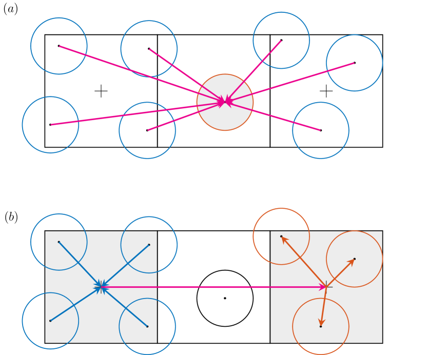
Figure 1: Illustration of the far product in the MLFMA-SME. (a) Particle-particle interaction on level $L_{\max}$. (b) Level $L_{\max}-1$, where $L_{\max}$ is the finest level.

At the finest level, standard Quadtree/Octree approaches might divide a meta-atom into different groups, making the grouping of entire-domain basis functions ambiguous. Leveraging the fact that we deal with meta-atoms whose dimensions are smaller than the wavelength, we propose grouping basis functions by considering each particle as a finest-level group, as shown in Fig. 1(a). At this level, all static modes $\bm{\psi}^{\mu}_{i}$ are physically associated with the center of the particle $\Omega_{\mu}$. For coarser levels, we hierarchically group the basis functions using a standard Quadtree structure (Fig. 1b), which is particularly suitable for structures where the lateral dimensions significantly exceed the vertical ones, as in the case of metasurfaces and metalenses.

Following the fast multipole prescriptions, we decompose the impedance matrix $Z$ as the sum of its block-diagonal part (near part) and the off-diagonal part (far part). For identical particles, the self-particle blocks $Z^{\mu\mu}$ are identical, i.e. $Z^{\mu\mu}=Z_{s}$ for $\mu=1,...,p$. Therefore, $Z_{s}$ can be evaluated and stored once, leading to significant savings in memory requirements and CPU time. To address the singularities in Green’s function when $\mathbf{r}=\mathbf{r}^{\prime}$, the numerical integration of shape function times Green’s function or its gradient are evaluated using the techniques introduced in Refs. [32] and [33].

According to (10), the far-field part of $Z$ is

$$Z^{\mu\nu}=\begin{bmatrix}\zeta^{-}T_{-}^{\mu\nu}&K_{-}^{\mu\nu}\\ -K_{-}^{\mu\nu}&\frac{1}{\zeta^{-}}T_{-}^{\mu\nu}\end{bmatrix}\hskip 21.52771pt\mbox{with}\;\mu\neq\nu,$$ (27)

with $\mu,\nu=1,...,p$. Since only $k^{-}$ appears when $\mu\neq\nu$, in the following we simplify the notations by omitting the ”$-$” symbol, thus $k=k^{-}$.

To evaluate the operators $T^{\mu\nu}$ and $K^{\mu\nu}$ when $\Omega_{\mu}$ is far from $\Omega_{\nu}$ (i.e. $\mu\neq\nu$), we rewrite the equations (5) and (6) as

$$T_{mn}^{\mu\nu}=-jk\int_{\partial\Omega_{\mu}}\bm{\psi}_{m}^{\mu}(\mathbf{r})\cdot\int_{\partial\Omega_{\nu}}\overset{\text{\scalebox{0.7}{{\hbox{\bm{\leftrightarrow}}}}}}{\mathbf{G}}(\mathbf{r},\mathbf{r}^{\prime})\bm{\psi}_{n}^{\nu}(\mathbf{r^{\prime}})\,\mathrm{d}S^{\prime}\,\,\mathrm{d}S,$$ (28)

$$K_{mn}^{\mu\nu}=\int_{\partial\Omega_{\mu}}\bm{\psi}_{m}^{\mu}(\mathbf{r})\cdot\int_{\partial\Omega_{\nu}}\bm{\psi}_{n}^{\nu}(\mathbf{r^{\prime}})\times\nabla^{\prime}g(\mathbf{r}-\mathbf{r}^{\prime})\,\mathrm{d}S^{\prime}\,\,\mathrm{d}S,$$ (29)

where $\overset{\text{\scalebox{0.7}{$\bm{\leftrightarrow}$}}}{\mathbf{G}}$ is the dyadic Green’s function

$$\overset{\text{\scalebox{0.7}{{\hbox{\bm{\leftrightarrow}}}}}}{\mathbf{G}}(\mathbf{r},\mathbf{r}^{\prime})=\left(\overset{\text{\scalebox{0.7}{{\hbox{\bm{\leftrightarrow}}}}}}{\mathbf{I}}-\frac{1}{{k}^{2}}\nabla\nabla^{\prime}\right)g(\mathbf{r}-\mathbf{r}^{\prime}),$$ (30)

and $\overset{\text{\scalebox{0.7}{$\bm{\leftrightarrow}$}}}{\mathbf{I}}$ is the unit dyad. Then, using the addition theorem [6], Green’s function can be expressed as

$$\frac{e^{-jk\|\mathbf{r}-\mathbf{r}^{\prime}\|}}{4\pi\|\mathbf{r}-\mathbf{r}^{\prime}\|}=\\ \int_{\mathbb{S}^{2}}e^{-jk\hat{\mathbf{k}}\cdot(\mathbf{r}-\mathbf{r}_{\mu})}T_{L}(\hat{\mathbf{k}},\mathbf{r}_{\mu\nu})e^{jk\hat{\mathbf{k}}\cdot(\mathbf{r}^{\prime}-\mathbf{r}_{\nu})}\mathrm{d}\hat{\mathbf{k}},$$ (31)

with $\mathbf{r}\in\Omega_{\mu}$, $\mathbf{r}^{\prime}\in\Omega_{\nu}$, $\mathbf{r}_{\mu\nu}=\mathbf{r}_{\mu}-\mathbf{r}_{\nu}$, where $\mathbf{r}_{\mu}$ and $\mathbf{r}_{\nu}$ are, respectively, the centers of the particles $\Omega_{\mu}$ and $\Omega_{\nu}$, $\mathbb{S}^{2}=\{\hat{\mathbf{k}}\in\mathbb{R}^{3}:\|\hat{\mathbf{k}}\|_{2}=1\}$ is the unit sphere, $T_{L}$ is the translation function [6, 34, 35, 31]

$$T_{L}(\hat{\mathbf{k}},\mathbf{r}_{\mu\nu})=\\ -\frac{jk}{(4\pi)^{2}}\sum_{\ell=0}^{L}(-j)^{\ell}(2\ell+1)h_{\ell}^{(2)}(k\|\mathbf{r}_{\mu\nu}\|)P_{\ell}(\hat{\mathbf{k}}\cdot\hat{\mathbf{r}}_{\mu\nu}),$$ (32)

where $h_{\ell}^{(2)}$ is the second kind spherical Hankel function of order $\ell$, $P_{\ell}$ is the Legendre Polynomial of order $\ell$.

Using the expansion (31) in Eqs. (28) and (29), we obtain

$$T^{\mu\nu}_{mn}=-jk\int_{\mathbb{S}^{2}}\bm{\hat{\psi}}^{\mu}_{m}(\hat{\mathbf{k}})\cdot T_{L}(\hat{\mathbf{k}},\mathbf{r}_{\mu\nu})(\overset{\text{\scalebox{0.7}{{\hbox{\bm{\leftrightarrow}}}}}}{\mathbf{I}}-\hat{\mathbf{k}}\hat{\mathbf{k}})\cdot\bm{\hat{\psi}}^{\nu*}_{n}(\hat{\mathbf{k}})\,\mathrm{d}\hat{\mathbf{k}},$$ (33)

$$K^{\mu\nu}_{mn}=-jk\int_{\mathbb{S}^{2}}\hat{\mathbf{k}}\times\bm{\hat{\psi}}^{\mu}_{m}(\hat{\mathbf{k}})\cdot T_{L}(\hat{\mathbf{k}},\mathbf{r}_{\mu\nu})\bm{\hat{\psi}}^{\nu*}_{n}(\hat{\mathbf{k}})\ \mathrm{d}\hat{\mathbf{k}},$$ (34)

where and $\bm{\hat{\psi}}^{\mu}_{m}$ is the $k$-space representation of the basis function

$$\bm{\hat{\psi}}^{\mu}_{m}(\hat{\mathbf{k}})=\int_{\partial\Omega_{\mu}}\bm{\psi}_{m}^{\mu}(\mathbf{r})e^{-jk\hat{\mathbf{k}}\cdot(\mathbf{r}-\mathbf{r}_{\mu})}\,\mathrm{d}S.$$ (35)

It is well known that truncating the series (32) at a finite order $L$ requires careful handling due to numerical instabilities caused by the nature of spherical Hankel functions [36, 34, 35, 37, 38]. Ideally, one would choose a high order to minimize error, but these functions are highly oscillatory at higher order, meaning that increasing $L$ does not necessarily enhance accuracy [39]. Furthermore, these functions diverge at small arguments, that is, when the electrical distance between two centers is too small, leading to a low-frequency breakdown [34, 39]. However, in this field of application, such instabilities are not observed at optical frequencies, because the particles are not too close together.

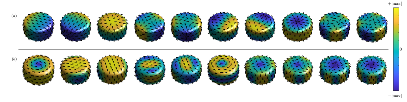
Figure 2: (a) First ten longitudinal static modes of a nanodisk. The arrows represent the direction of the surface current density field, the colors represent the surface charge density. (b) First ten transverse static modes of a nanodisk. The arrows represent the direction of the surface current density field, the colors represent the magnitude of the current density field. Modes are presented in ascending lexicographic order and sorted according to their respective static eigenvalues.

V Results and Discussion

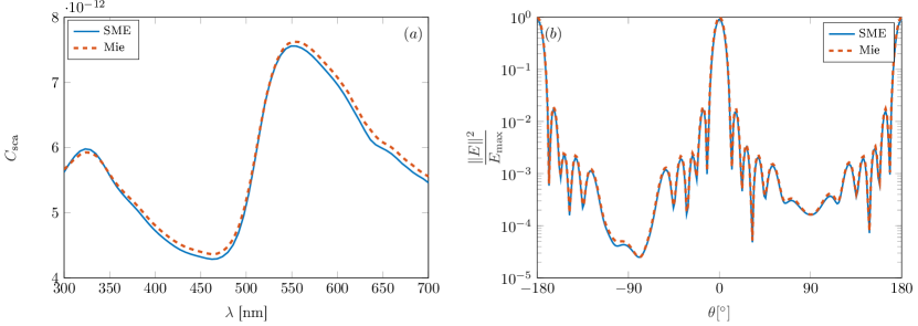
Figure 3: (a) Scattering cross section of a finite Vogel spiral composed of 100 gold spheres of radius $R=100$ nm under the excitation of a linearly polarized plane wave at wavelength $\lambda$. $C_{sca}$ is computed using the MLFMA-SME with $N^{\|}=N^{\perp}=10$. (b) Normalized scattered far field at $\lambda$ = 600 nm. The reference Mie solution (dashed line) is also provided for comparison.

The execution of the numerical algorithm can be subdivided into five stages:

• Assembly of the self-interaction impedance matrix $Z_{s}$ of an individual meta-atom and the right-hand side vector $\mathbf{V}$ using RWG basis functions. Since the particles are identical, $Z_{s}$ only needs to be evaluated and stored once. The computational complexity and memory requirement for assembling and storing $Z_{s}$, in terms of the number of particles, is $(2n_{e})^{2}\mathcal{O}(1)$.

• Generation of the static modes of an isolated object. Specifically, the longitudinal static modes are obtained by solving the eigenvalue problem (18) using star functions as both expansion and testing functions; the transverse static modes are obtained by solving the eigenvalue problem (21) using loop functions as both expansion and testing functions. In Fig. 2, we present the calculated first ten longitudinal and ten transverse static modes for a nanodisk.

• Evaluation of the MLFMA operators, consisting of the translation function $T_{L}$, the radiation and receive operators $\bm{\hat{\psi}}$ and $\bm{\hat{\psi}}^{\dagger}$. The time complexity and memory requirements for assembling $T_{L}$ are on the order of $\mathcal{O}(p\log p)$. Since the operators $\bm{\hat{\psi}}$ and $\bm{\hat{\psi}}^{\dagger}$ are evaluated for each particle, their time and memory complexities are on the order of $\mathcal{O}(p)$. These complexities can be reduced to $\mathcal{O}(1)$ if the particles have the same spatial orientation (i.e., there is no rotation between particles).

• Compression stage, i.e. transitioning from the representation of the matrices $Z_{s}$, $\bm{\hat{\psi}}$ and $\bm{\hat{\psi}}^{\dagger}$ in terms of the RWG basis to the representation in terms of the static modes basis. This stage can be integrated into steps i) and iii), as there is no need to directly store the RWG representation of these operators.

• Solution of the PMCHWT system using an iterative method accelerated by the Multilevel Fast Multipole Algorithm (MLFMA), which reduces the computational complexity of the matrix-vector product from $\mathcal{O}(p^{2})$ to $\mathcal{O}(p\log p)$. This stage is the most time-consuming, as the entire system is solved with a complexity of $\mathcal{O}(Ip\log p)$, where $I$ is the number of iterations required. To accelerate the convergence of the Generalized Minimal Residual Method (GMRES) [40], we employ a block-diagonal preconditioner, where each block is the single-particle self-interaction impedance matrix. We choose a relative tolerance of $10^{-4}$. It effectively reduces $I$ to $\mathcal{O}(p^{\alpha})$, with $\alpha<1$.

In the following simulations, the truncation number $L$ of the translation function (32), is initially set to $10$ at the finest level. This value is subsequently doubled at each successive level [6]. The numerical evaluation of the integrals over the unit sphere is performed using $K=2L^{2}$ point [6]. For interpolation, we employ a $4\times 4$ Lagrange interpolation scheme. The FORTRAN code used to implement this algorithm operates on a single CPU (Intel Xeon-Gold 6140 M 2.3 GHz).

V.1 Validation

We validate the MLFMA-SME method by investigating the scattering from a particle array composed of 100 identical gold nano-spheres, each of radius $R=100$ nm, and arranged according to a golden angle spiral pattern [41]. The $i$-th particle is centered at $(x_{i},y_{i})$, according to

$$\begin{cases}x_{i}=r_{i}\cos(i\alpha)\\ y_{i}=r_{i}\sin(i\alpha),\\ \end{cases}$$ (36)

where $i=1,...,p$; $r_{i}=c\sqrt{i}$, $c$ is a constant scaling factor, $\alpha=2\pi/\phi^{2}$ is the golden angle, where $\phi=(1+\sqrt{5})/2$ is the golden ratio. We choose the scaling factor as $c=\sqrt{3}R$.

The gold permittivity is obtained by interpolating experimental data [42]. The array is illuminated by a linearly polarized plane, propagating along the axis orthogonal to the array’s plane, linearly polarized along the $x$-axis, with varying wavelength $\lambda$ in the interval $[300,700]$nm. Each particle’s surface is discretized by a triangular mesh having $500$ nodes, $996$ triangles, and $1494$ edges. The scattering cross section, $C_{sca}$, is plotted in Fig. 3 a as function of $\lambda$. The solution, computed by the MLFMA-SME, utilizing $N^{\|}=N^{\perp}=10$ modes per particle, corresponding to a total number of $4000$ unknowns, is compared against the multiparticle Mie theory [19], where the field expansions are truncated at the order $M=15$. The relative error on the scattering cross section is defined as

$$\epsilon\{C_{sca}\}=\frac{|C_{sca}-\bar{C}_{sca}|}{\bar{C}_{sca}},$$ (37)

where $\bar{C}_{sca}$ is the reference solution obtained by the multiparticle Mie theory. The achieved error is lower than $0.02$ all over the investigated spectral range.

For the same array, in Fig. 3b we show the normalized scattered far field for a fixed wavelength $\lambda=600$ nm. The reference Mie solution, obtained for $M=30$, is included for comparison. An excellent agreement is found.

V.2 Computational costs

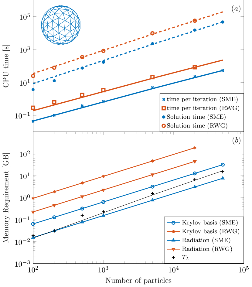
Figure 4: (a) CPU time required for the PMCHWT system solution, comparing the RWG with Static Mode Expansion. The code is implemented in FORTRAN and runs on a single CPU. (b) Memory requirement comparison between the RWG with Static Mode Expansion. The $\mathcal{O}(p\log p)$ (continuous line) and $\mathcal{O}\left(p^{1.25}\log p\right)$ (dashed line) curves are also plotted for reference. (Inset) Surface mesh used for the computational complexity test.

We conducted a complexity study on metasurfaces consisting of a varying number up to $5\cdot 10^{4}$ of identical gold nano-spheres, each of radius R = 100 nm. The particles are arranged according to a golden-angle spiral pattern. This aperiodic pattern is particularly convenient for our study as it is deterministic, and allows us to increase the dimension of the array one particle at a time without appreciably changing the array’s density. The array is excited by a linearly polarized plane wave of wavelength $\lambda=600$ nm, propagating along the axis orthogonal to the array’s plane. Each sphere has been discretized by a surface mesh, shown in the inset of Fig. 4 (a), with $100$ nodes, $196$ triangles, $294$ edges, which results in an average edge length approximately equal to $\lambda/15$. In Fig 4, we present a comparison between the CPU time and memory requirements using the MLFMA with RWG basis function and static mode expansion with $N^{\|}=N^{\perp}=10$. Simulation results show that the use of MLFMA, in both cases RWG and SME, reduces the computational complexity of the matrix-vector product from $\mathcal{O}(p^{2})$ to $\mathcal{O}(p\log p)$, as expected. The number of degrees of freedom, and the computational time of each case study reported in Fig. 4 are listed in Tab. 1. In particular, with the use of the SME, this simulation is approximately $3\div 5$ times faster.

However, the speed-up depends on various factors, such as the number of points used for interpolation/anterpolation between different levels of the quadtree, or the number of points used to sample the transfer function $T_{L}$ on the unit sphere. Above all, mesh density on each particle plays a very important role. Indeed, the advantages introduced by the MLFMA-SME become much more apparent with denser meshes, necessary for discretizing irregular objects, such as nanofins and nanorods typically used in metalens. The reason why the speed-up is less than the number of unknowns’ compression ratio is attributable to the $k$-space representation of the MLFMA operators, which means that the computational complexity is not only linked to the number of unknowns but also to the electrical size of the array.

Table 1: Comparison between RWG and SME.

	Total Number		Time per		Total GMRES		Number of
$p$	of Unknowns		iteration [s]		time [min]		iterations
	RWG	SME	RWG	SME	RWG	SME	RWG	SME
100	$5.880\cdot 10^{4}$	$4\cdot 10^{3}$	0.29	0.04	0.42	0.06	85	84
200	$1.176\cdot 10^{5}$	$8\cdot 10^{3}$	0.62	0.10	1.32	0.21	127	126
500	$2.940\cdot 10^{5}$	$2\cdot 10^{4}$	1.78	0.38	5.82	1.25	196	195
1000	$5.880\cdot 10^{5}$	$4\cdot 10^{4}$	3.37	0.70	13.84	2.85	246	243
5000	$2.940\cdot 10^{6}$	$2\cdot 10^{5}$	20.95	4.92	161.34	37.61	462	458
20000	$1.176\cdot 10^{7}$	$8\cdot 10^{5}$	83.88	22.67	939.46	253.51	672	671
50000	-	$2\cdot 10^{6}$	-	53.32	-	782.08	-	880

Another crucial advantage introduced by SME in the MLFMA concerns memory requirements. Although the translation function $T_{L}$ is the same in both RWG and SME, as it doesn’t depend on the basis function, the matrices representing the radiation and receive operators are $\kappa$ times smaller, and the self impedance matrix $Z_{s}$ is $\kappa^{2}$ times smaller, where $\kappa=n_{e}/(N^{\parallel}+N^{\perp})$ is the total number of unknowns’ compression ratio. Additionally, after $m$ iterations, computing the GMRES solution requires storing all the basis vectors of the Krylov subspace $\mathcal{K}_{m}$, leading to a memory requirement of $\mathcal{O}(mN)$, where $N$ is the total number of unknowns. As $N$ increases, the storage cost may become prohibitive, even for a small number of iterations $m$. As previously mentioned, SME can drastically reduce $N$, allowing for the simulation of larger structures that were impracticable before.

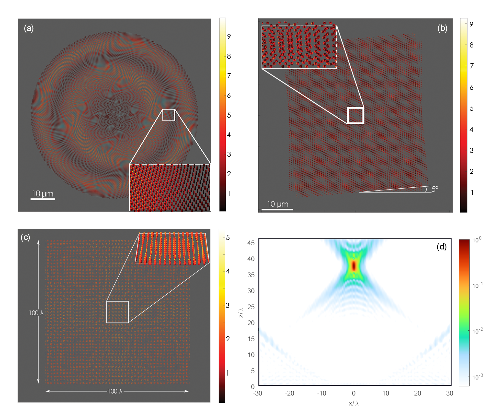
Figure 5: (a) Electric field magnitude on the particles’ surface of a finite Vogel spiral composed of $40\cdot 10^{3}$ gold bricks of dimension $200\times 200\times 100$ nm under the excitation of a linearly polarized plane wave at wavelength $\lambda$ = 600 nm. The array size is about $70\mu$m, which is roughly $115\lambda$. The solution has been computed by using the MLFMA-SME with $N^{\|}=N^{\perp}=10$. (b) Electric field magnitude on the particles’ surface of a Moiré superlattice array composed of 20160 gold nanodisks of radius $100$ nm under the excitation of a linearly polarized plane wave at wavelength $\lambda$ = 600 nm. The array size is about $46\times 53\mu$m, which is roughly $(76\times 87)\lambda$. The solution has been computed by using the MLFMA-SME with $N^{\|}=N^{\perp}=10$. (c) Electric field magnitude on the particles’ surface of a canonical metalens, lying on the xy plane, and composed of $10^{4}$ $\mathrm{TiO}_{2}$ nanofins of dimension $410\times 85\times 600$ nm under the excitation of a circularly polarized plane wave at wavelength $\lambda=660$ nm. The array size is $66\,\mu$m, which is $100\lambda$. The solution has been computed by using the MLFMA-SME with $N^{\|}=N^{\perp}=10$. (d) Electric field normalized intensity on the $x-z$ cross-sectional plane. The achieved focal length is consistent with the prescribed value of $f=37.5\lambda$.

V.3 Electrically large particle arrays

The use of the MLFMA-SME finds its natural application in the numerical solution of the electromagnetic scattering problem by large metasurfaces, where an array, whose dimension can be much larger than the incident wavelength, is made of $p$ objects with identical shape but with different orientation and size. We show three exemplificative case studies of the application of this method to metasurfaces and metalenses: a golden angle spiral of gold bricks, and a Moirè lattice of gold disks and a canonical metalens of $\text{TiO}_{2}$ nano-fins.

In all three cases, we model the shape of the meta-atoms as a superellipsoid, whose boundary has the implicit equation

$$\left[\left(\frac{x}{a_{x}}\right)^{\frac{2}{m}}+\left(\frac{y}{a_{y}}\right)^{\frac{2}{m}}\right]^{\frac{m}{n}}+\left(\frac{z}{a_{z}}\right)^{\frac{2}{n}}-1=0,$$ (38)

We used the public domain code developed by Per-Olof Persson and Gilbert Strang [43] to generate the surface mesh.

We first consider a finite-size golden angle spiral array having linear dimension of $115\lambda$. The array is made of $40\cdot 10^{3}$ gold bricks of dimension $200\times 200\times 100$ nm. We model this shape as a superellipsoid, using Eq. (38) with $m=n=0.25$, $a_{x}=a/2$, $a_{y}=a_{z}=a$. Each particle is described by a surface mesh having $436$ nodes, $868$ triangles, and $1302$ edges. The $i$-th particle is rotated with respect to $\hat{\mathbf{x}}$ by an angle $\theta_{i}=2\pi(i-1)/p$. The array is excited by a plane wave, linearly polarized in the plane of the array, along the $\hat{\mathbf{x}}$-axis, and propagating in the direction orthogonal to the array’s plane with wavelength $\lambda=600$ nm. The array size is about $70\mu$m. In Fig. 5a, we show the electric field magnitude on the particles’ surface. The solution is computed by using the MLFMA-SME as detailed in this work using the static mode expansion with $N^{\|}=N^{\perp}=10$, i.e. 40 unknowns per particle. The total computational time is about 20.4 hours on a single CPU.

Next, we now consider an example of 2.5D metastructures, which are stacked layers of interacting metasurface layers. They provide sufficient degrees of freedom to implement efficient multifunctional devices. Specifically, we consider a two-layer Moiré superlattice array of $20160$ gold nanodisks of radius $R=100$ nm. We model this shape as a superellipsoid, whose boundary has the implicit equation (38), with $m=1$, $n=0.25$, $a_{x}=a_{y}=R$, $a_{z}=R/2$. Each particle is described by a surface mesh having $588$ nodes, $1172$ triangles, and $1758$ edges. The centers of the particles are arranged at the vertices of two layers, obtained by periodically replicating a hexagon with a side length of $400$ nm. The second layer is located at a height $h=300$ nm above the first and is rotated by an angle $\theta=5$° with respect to it. The array is excited by a plane wave, linearly polarized in the plane of the array, along the $\hat{\mathbf{x}}$-axis, and propagating in the direction orthogonal to the array’s plane with wavelength $\lambda=600$ nm. The array size is about $46\times 53\,\mu$m, which is roughly $(76\times 87)\lambda$. In Fig. 5b we show the electric field magnitude on the particles’ surface, while in Fig. 2 we show the longitudinal and transverse modes. The solution is computed using the MLFMA-SME with $N^{\|}=N^{\perp}=10$. The total computational time is less than 6 hours on a single CPU.

Eventually, we consider an example of a canonical metalens [13], composed of $10^{4}$ $\mathrm{TiO}_{2}$ nanofins of dimension $410\times 85\times 600$ nm. We model this shape as a superellipsoid, whose boundary has the implicit equation (38), with $m=n=0.25$. The total computational time is about 15 hours on a single CPU. Each particle is described by a surface mesh having $198$ nodes, $392$ triangles, and $588$ edges. To achieve the desired phase profile, the $i$-th particle, centered at $(x_{i},y_{i})$, is rotated with respect to $\hat{\mathbf{x}}$ by an angle [13, 44]

$$\theta_{i}=\frac{\pi}{\lambda}\left(f-\sqrt{f^{2}+x_{i}^{2}+y_{i}^{2}}\right),$$ (39)

where $f$ is the focal length. The metalens has a desired numerical aperture (NA) of 0.8, resulting in a focal length $f=37.5\lambda$. The array is excited by a plane wave, circularly polarized in the plane of the array and propagating in the direction orthogonal to the array’s plane with wavelength $\lambda=660$ nm. The array size is $66\times 66\,\mu$m, which is $(100\times 100)\lambda$. In Fig. 5c we show the electric field magnitude on the particles’ surface. The solution is computed using the MLFMA-SME with $N^{\|}=N^{\perp}=10$. In Fig. 5d we show the normalized intensity $\|\mathbf{E}(x,z)\|^{2}$ on the $x-y$ cross-sectional plane. The achieved focal length is consistent with the prescribed value.

VI Conclusion

In this work, we proposed a fast integral equation solver suitable for large particle arrays, even those hundreds of wavelengths in diameter, comprising numerous arbitrarily shaped objects with varying orientations and sizes. These scenarios are commonly encountered in the electromagnetic modeling of metasurfaces and metalenses. Our approach combines the Multilevel Fast Multipole Algorithm (MLFMA) with the PMCHWT formulation, utilizing a particular class of entire domain basis function defined on the isolated particle, termed Static Mode [18].

To validate the accuracy of the proposed method, we analyze the scattering from finite aperiodic arrays of nano-spheres and compare the results with those obtained using the multiparticle Mie theory [19]. We report the CPU-time and memory requirements as functions of the number of particles, comparing the static mode expansion to a more traditional approach using RWG basis functions. Our findings indicate that the MLFMA-SME is $3$ to $5$ times faster and requires about $5$ times less memory than the traditional MLFMA employing RWG basis functions. Furthermore, this speed and memory advantages significantly improve as the density of the surface mesh increases.

Additionally, we demonstrate the capabilities of the MLFMA-SME method on different arrays: a golden-angle spiral array with a diameter of $115\lambda$, consisting of 40,000 gold bricks; a two-layer Moiré superlattice made up of 20,160 gold nanodisks, with overall dimensions of $76\lambda\times 87\lambda$; a canonical metalens composed of 10,000 $\mathrm{TiO}_{2}$ nanofins, covering an area of $100\lambda\times 100\lambda$ and having focal length $f=37.5\lambda$.

Our results show that SME drastically reduces the total number of unknowns, leading to significant savings in CPU time and memory requirements for the numerical solution of scattering problems from arrays of identical particles compared to the classical MLFMA implementation with sub-domain basis functions. This advancement enables the simulation of large structures that were previously impracticable.

- [1] A. Silva, F. Monticone, G. Castaldi, V. Galdi, A. Alù, and N. Engheta, “Performing mathematical operations with metamaterials,” Science, vol. 343, no. 6167, pp. 160–163, 2014.
- [2] N. Yu and F. Capasso, “Flat optics with designer metasurfaces,” Nature Materials, vol. 13, pp. 139–150, Feb. 2014. Bandiera_abtest: a Cg_type: Nature Research Journals Number: 2 Primary_atype: Reviews Publisher: Nature Publishing Group Subject_term: Metamaterials Subject_term_id: metamaterials.
- [3] F. Aieta, M. A. Kats, P. Genevet, and F. Capasso, “Multiwavelength achromatic metasurfaces by dispersive phase compensation,” Science, vol. 347, pp. 1342–1345, Mar. 2015. Publisher: American Association for the Advancement of Science.
- [4] W. Xue, H. Zhang, A. Gopal, V. Rokhlin, and O. D. Miller, “Fullwave design of cm-scale cylindrical metasurfaces via fast direct solvers,” Aug. 2023. arXiv:2308.08569 [physics].
- [5] L. Greengard and V. Rokhlin, “A fast algorithm for particle simulations,” Journal of Computational Physics, vol. 73, pp. 325–348, Dec. 1987.
- [6] W. C. Chew, J.-M. Jin, E. Michielssen, and J. Song, eds., Fast and Efficient Algorithms in Computational Electromagnetics. Boston: Artech House, July 2000.
- [7] J. Fostier and F. Olyslager, “An Asynchronous Parallel MLFMA for Scattering at Multiple Dielectric Objects,” IEEE Transactions on Antennas and Propagation, vol. 56, pp. 2346–2355, Aug. 2008. Conference Name: IEEE Transactions on Antennas and Propagation.
- [8] K. Donepudi, J.-M. Jin, S. Velamparambil, J. Song, and W. C. Chew, “A higher order parallelized multilevel fast multipole algorithm for 3-D scattering,” IEEE Transactions on Antennas and Propagation, vol. 49, pp. 1069–1078, July 2001. Conference Name: IEEE Transactions on Antennas and Propagation.
- [9] S. Velamparambil and W. C. Chew, “Analysis and performance of a distributed memory multilevel fast multipole algorithm,” IEEE Transactions on Antennas and Propagation, vol. 53, pp. 2719–2727, Aug. 2005. Conference Name: IEEE Transactions on Antennas and Propagation.
- [10] O. Ergül and L. Gürel, “Fast and accurate analysis of optical metamaterials using surface integral equations and the parallel multilevel fast multipole algorithm,” in 2013 International Conference on Electromagnetics in Advanced Applications (ICEAA), pp. 1309–1312, Sept. 2013.
- [11] C. Waltz, K. Sertel, M. A. Carr, B. C. Usner, and J. L. Volakis, “Massively Parallel Fast Multipole Method Solutions of Large Electromagnetic Scattering Problems,” IEEE Transactions on Antennas and Propagation, vol. 55, pp. 1810–1816, June 2007. Conference Name: IEEE Transactions on Antennas and Propagation.
- [12] A. Fijany, M. Jensen, Y. Rahmat-Samii, and J. Barhen, “A massively parallel computation strategy for FDTD: time and space parallelism applied to electromagnetics problems,” IEEE Transactions on Antennas and Propagation, vol. 43, pp. 1441–1449, Dec. 1995. Conference Name: IEEE Transactions on Antennas and Propagation.
- [13] T. W. Hughes, M. Minkov, V. Liu, Z. Yu, and S. Fan, “A perspective on the pathway toward full wave simulation of large area metalenses,” Applied Physics Letters, vol. 119, p. 150502, Oct. 2021.
- [14] Y. Chang and R. Harrington, “A surface formulation for characteristic modes of material bodies,” IEEE Transactions on Antennas and Propagation, vol. 25, pp. 789–795, Nov. 1977. Conference Name: IEEE Transactions on Antennas and Propagation.
- [15] T.-K. Wu and L. L. Tsai, “Scattering from arbitrarily-shaped lossy dielectric bodies of revolution,” Radio Science, vol. 12, no. 5, pp. 709–718, 1977.
- [16] A. J. Poggio and E. K. Miller, “CHAPTER 4 - Integral Equation Solutions of Three-dimensional Scattering Problems,” in Computer Techniques for Electromagnetics (R. Mittra, ed.), International Series of Monographs in Electrical Engineering, pp. 159–264, Pergamon, Jan. 1973.
- [17] R. F. Harrington, Field computation by moment methods. Wiley-IEEE Press, 1993.
- [18] C. Forestiere, G. Gravina, G. Miano, G. Rubinacci, and A. Tamburrino, “Static Surface Mode Expansion for the Electromagnetic Scattering From Penetrable Objects,” IEEE Transactions on Antennas and Propagation, vol. 71, pp. 6779–6793, Aug. 2023. Conference Name: IEEE Transactions on Antennas and Propagation.
- [19] Y. Xu, “Electromagnetic scattering by an aggregate of spheres,” Appl. Opt., vol. 34, no. 21, pp. 4573–4588, 1995.
- [20] S. Rao, D. Wilton, and A. Glisson, “Electromagnetic scattering by surfaces of arbitrary shape,” IEEE Transactions on Antennas and Propagation, vol. 30, pp. 409–418, May 1982. Conference Name: IEEE Transactions on Antennas and Propagation.
- [21] C. Forestiere, G. Gravina, G. Miano, M. Pascale, and R. Tricarico, “Electromagnetic modes and resonances of two-dimensional bodies,” Physical Review B, vol. 99, p. 155423, Apr. 2019. Publisher: American Physical Society.
- [22] P. Monk, Finite Element Methods for Maxwell’s Equations. Clarendon Press, Apr. 2003.
- [23] D. Wilton, J. Lim, and S. Rao, “A novel technique to calculate the electromagnetic scattering by surfaces of arbitrary shape,” URSI Radio Science Meeting, p. 322, 1993.
- [24] M. Burton and S. Kashyap, “A study of a recent, moment-method algorithm that is accurate to very low frequencies,” Applied Computational Electromagnetics Society Journal, vol. 10, pp. 58–68, 1995.
- [25] O. M. Bucci and G. D. Massa, “Use of characteristic modes in multiple-scattering problems,” Journal of Physics D: Applied Physics, vol. 28, pp. 2235–2244, Nov. 1995.
- [26] R. Garbacz, “Modal expansions for resonance scattering phenomena,” Proceedings of the IEEE, vol. 53, pp. 856–864, Aug. 1965. Conference Name: Proceedings of the IEEE.
- [27] R. Harrington, J. Mautz, and Yu Chang, “Characteristic modes for dielectric and magnetic bodies,” IEEE Transactions on Antennas and Propagation, vol. 20, pp. 194–198, Mar. 1972.
- [28] Y. Chen and C.-F. Wang, Characteristic Modes: Theory and Applications in Antenna Engineering. John Wiley & Sons, June 2015.
- [29] N. Engheta, W. Murphy, V. Rokhlin, and M. Vassiliou, “The fast multipole method (FMM) for electromagnetic scattering problems,” IEEE Transactions on Antennas and Propagation, vol. 40, pp. 634–641, June 1992.
- [30] R. Coifman, V. Rokhlin, and S. Wandzura, “The fast multipole method for the wave equation: a pedestrian prescription,” IEEE Antennas and Propagation Magazine, vol. 35, pp. 7–12, June 1993. Conference Name: IEEE Antennas and Propagation Magazine.
- [31] J. Song, C.-C. Lu, and W. C. Chew, “Multilevel fast multipole algorithm for electromagnetic scattering by large complex objects,” IEEE Transactions on Antennas and Propagation, vol. 45, pp. 1488–1493, Oct. 1997. Conference Name: IEEE Transactions on Antennas and Propagation.
- [32] R. Graglia, “On the numerical integration of the linear shape functions times the 3-D Green’s function or its gradient on a plane triangle,” Antennas and Propagation, IEEE Transactions on, vol. 41, pp. 1448 –1455, Oct. 1993.
- [33] R. E. Hodges and Y. Rahmat-Samii, “The evaluation of MFIE integrals with the use of vector triangle basis functions,” Microwave and Optical Technology Letters, vol. 14, no. 1, pp. 9–14, 1997.
- [34] J. Song and W. C. Chew, “Error analysis for the truncation of multipole expansion of vector Green’s functions [EM scattering],” IEEE Microwave and Wireless Components Letters, vol. 11, pp. 311–313, July 2001. Conference Name: IEEE Microwave and Wireless Components Letters.
- [35] M. L. Hastriter, S. Ohnuki, and W. C. Chew, “Error control of the translation operator in 3D MLFMA,” Microwave and Optical Technology Letters, vol. 37, no. 3, pp. 184–188, 2003.
- [36] M. Abramowitz and I. A. Stegun, Handbook of Mathematical Functions with Formulas, Graphs, and Mathematical Tables. New York: Dover, ninth dover printing ed., 1964.
- [37] S. Koc, J. Song, and W. Chew, “Error analysis for the multilevel fast multipole algorithm,” in IEEE Antennas and Propagation Society International Symposium. 1998 Digest. Antennas: Gateways to the Global Network. Held in conjunction with: USNC/URSI National Radio Science Meeting (Cat. No.98CH36, vol. 3, pp. 1758–1761 vol.3, June 1998.
- [38] B. Dembart and E. Yip, “The accuracy of fast multipole methods for Maxwell’s equations,” IEEE Computational Science and Engineering, vol. 5, pp. 48–56, July 1998. Conference Name: IEEE Computational Science and Engineering.
- [39] E. Darve and P. Havé, “Efficient fast multipole method for low-frequency scattering,” Journal of Computational Physics, vol. 197, pp. 341–363, June 2004.
- [40] Y. Saad and M. H. Schultz, “GMRES: A Generalized Minimal Residual Algorithm for Solving Nonsymmetric Linear Systems,” SIAM Journal on Scientific and Statistical Computing, vol. 7, pp. 856–869, July 1986. Publisher: Society for Industrial and Applied Mathematics.
- [41] J. Trevino, H. Cao, and L. Dal Negro, “Circularly Symmetric Light Scattering from Nanoplasmonic Spirals,” Nano Letters, vol. 11, pp. 2008–2016, May 2011. Publisher: American Chemical Society.
- [42] P. B. Johnson and R. W. Christy, “Optical Constants of the Noble Metals,” Physical Review B, vol. 6, pp. 4370–4379, Dec. 1972.
- [43] P.-O. Persson and G. Strang, “A Simple Mesh Generator in Matlab,” SIAM Review, vol. 46, no. 2, pp. 329–345, 2004.
- [44] M. Khorasaninejad, W. T. Chen, R. C. Devlin, J. Oh, A. Y. Zhu, and F. Capasso, “Metalenses at visible wavelengths: Diffraction-limited focusing and subwavelength resolution imaging,” Science, vol. 352, no. 6290, pp. 1190–1194, 2016.