Confining modeling of quark propagator

Abstract

A confining extension of the quark model with nonlocal currents is proposed. The quark propagator is modified by introducing a cut in $\alpha$-space, which in momentum space corresponds to the subtraction of pole singularities. A two-phase phase structure is proposed for modeling the confinement-deconfinement phase transition. In the confined phase, the quark propagator does not have any pole singularities, while in the deconfined phase, there is a single quark pole.

I Introduction

Understanding of strong interactions is a complex task. The fundamental theory of strong interactions, quantum chromodynamics (QCD), is formulated in terms of quarks and gluons. Experimentally observed hadrons are interpreted as bound states of these fundamental constituents. This is due to the nonperturbative nature of QCD. The strong coupling constant $\alpha_{s}$ is a small parameter only at large $Q^{2}$. Free quarks and gluons have not been observed in experiments, they are confined inside hadrons. It is expected that under certain physical conditions, such as in heavy ion collisions or within neutron stars, a different state of matter may form, which differs from the hadronic world we know. In this state, fundamental particles become deconfined and can freely propagate as quarks and gluons in a quark-gluon plasma (QGP). The only ab-initio, nonperturbative method for investigating strong interactions is lattice QCD simulation. In recent years, lattice QCD has made impressive progress. Despite this, the theoretical understanding of the underlying degrees of freedom still requires modeling since lattice simulations only provide numerical results without deeper insight. The symmetries of strong interactions can serve as a guiding principle, such as chiral perturbation theory [1], which deals with Goldstone bosons or the quark version of Nambu-Jona-Lasinio (NJL) model [2], where chiral symmetry is spontaneously broken due to quark condensate and massive constituent quarks are formed instead of current ones.

More sophisticated approaches are based on coupled systems of Dyson–Schwinger equations (DSE) for quark and gluon propagators and their vertices, along with Bethe–Salpeter equations for hadronic bound states [3]. These approaches describe quarks with a momentum-dependent mass $m(k^{2})$ and wave-function renormalization $Z(k^{2})$. At large momentum transfer, the mass function tends to the current mass. The nonlocal version of the Nambu-Jona-Lasinio (NJL) model [4, 5] is somewhere between these two approaches. The structure of the interaction is similar to that of the NJL model, but the nonlocal quark current leads to a quark propagator with momentum-dependent mass

However, the absence of confinement can make calculations problematic. If the denominator of the quark propagator has zeroes

$${k^{2}+m^{2}(k^{2})}=0,$$ (1)

at real values, $k^{2}=-m^{2}_{\mathrm{pole}}$, this will result in an imaginary part in the polarization operators of mesons. This imaginary part corresponds to the appearance of free quarks. One way to avoid the occurrence of an imaginary component in polarization operators is to have a mass function $m(k^{2})$ that only results in complex-valued solutions of this equation. This case is similar to the scheme [6] and could be interpreted as modeling confinement [7]. Apart from technical issues in calculating Feynman diagrams, the physical meaning of complex singularities remains unclear. In a medium with varying temperature or baryon density, the positions of the singularities change, further complicating their physical interpretation.

In this paper, we aim to demonstrate that by making relatively simple modifications to the model, it is possible to eliminate these undesirable singularities. The general idea is that confinement should somehow change the model, which is based on chiral symmetry. Therefore, physical observables related to free quarks should not exist in the hadron phase. In addition, a method for realizing the confinement-deconfinement phase transition is required. It should be noted that the Polyakov loop extension of the NJL model with an effective potential of gauge degrees of freedom is intended to address one aspect of quark confinement at finite temperature – the suppression of quark pressure in the confining phase [8]. We propose an additional extension to the quark model. The inverse Laplace transform of the denominator of the quark propagator in the confined phase is modified to ensure that the transformed function is valid for arbitrary momentum. The resulting momentum space-transformed function has no pole singularities. The new momentum scale parameter associated with this modification can be interpreted as the confinement scale $\Lambda_{c}$. In the deconfined phase, a similar procedure is applied when the quark pole has been separated.

II Nonlocal model

The Lagrangian of the $SU(2)$ nonlocal chiral quark model with pseudoscalar–scalar sectors is:

$$\mathcal{L}=\mathcal{L}_{free}+\mathcal{L}_{P,S},\quad\mathcal{L}_{free}=\bar{q}(x)(i\hat{\partial}-M_{c})q(x),$$ (2)

$$\mathcal{L}_{P,S}=\frac{G}{2}\bigg{(}\Big{(}J_{S}^{a}(x)\Big{)}^{2}+\Big{(}J^{a}_{P}(x)\Big{)}^{2}\bigg{)},\quad$$ (3)

where $M_{c}=\mathrm{diag}(m_{c},m_{c})$ is the current quark mass matrix with diagonal elements $m_{c}$, $G$ is the four-quark coupling constant.

The nonlocal quark current can be taken in one-gluon-exchange-like (OGE) [4] or instanton liquid model (ILM) [9, 5] forms. The structure of OGE-type currents is:

$$J_{M}^{a\{,\mu\}}(x)=\int d^{4}x_{1}d^{4}x_{2}\,\delta\left(x-\frac{x_{1}+x_{2}}{2}\right)\times$$

$$\times g((x_{1}-x_{2})^{2})\,\bar{q}(x_{1})\,\Gamma_{M}^{a\{,\mu\}}\,q(x_{2}),$$ (4)

with $M=S,P$ and $\Gamma_{{S}}^{a}=\lambda^{a}$, $\Gamma_{{P}}^{a}=i\gamma^{5}\lambda^{a}$. For the $SU(2)$ model, the flavour matrices are Pauli matrices: $\lambda^{a}\equiv\tau^{a}$, $a=0,..,3$ with $\tau^{0}=1$. $g(x)$ is the form factor encoding the nonlocality of the QCD vacuum.

The bosonized Lagrangian after the Hubbard-Stratonovich transformation is:

$$\mathcal{L}_{eff} =\bar{q}(x)(i\hat{\partial}_{x}-M_{c})q(x)+\sigma_{0}J_{S}^{0}(x)+$$

$$-\frac{1}{2G}\left(\Big{(}P^{a}(x)\Big{)}^{2}+\Big{(}\tilde{S}^{a}(x)+\sigma_{0}\delta^{a}_{0}\Big{)}^{2}\right)+$$ (5)

$$+P^{a}(x)J_{P}^{a}(x)+\tilde{S}^{a}(x)J_{S}^{a}(x)$$

Spontaneous chiral symmetry breaking leads to non-zero vacuum expectation value of the scalar isoscalar field $\langle S^{0}\rangle_{0}=\sigma_{0}\neq 0$. After shifting the scalar isoscalar field $S^{0}=\tilde{S}^{0}+\sigma^{0}$, the momentum-dependent quark mass appears:

$$m(p^{2})=m_{c}+m_{d}g(p^{2})$$ (6)

where scalar coefficient $m_{d}=-\sigma^{0}$ can be found from self-consistent equation

$$m_{d}=G\frac{8N_{c}}{(2\pi)^{4}}\int d^{4}_{E}k\frac{g(k^{2})m(k^{2})}{k^{2}+m^{2}(k^{2})},$$ (7)

where $N_{c}$ is the number of quark colors. The quark propagator in Minkowski metric is

$$\mathrm{S}(p)=(\hat{p}-m(p))^{-1}.$$ (8)

The pion polarization loop is

$$\Pi_{\pi}(p^{2})=\frac{8N_{c}}{(2\pi)^{4}}\int d_{E}^{4}kf^{2}(q^{2})\,\mathrm{D}(k_{-}^{2})\mathrm{D}(k_{+}^{2})\times$$

$$\times\left[{(k_{-}\cdot k_{+})+m(k_{+}^{2})m(k_{-}^{2})}\right],$$ (9)

where $\mathrm{D}(k^{2})=(k^{2}+m^{2}(k^{2}))^{-1}$ is scalar propagator and momenta are $p=k_{+}-k_{-}$ and $q=(k_{+}+k_{-})/2$. In the general case, the flow of momentum in the diagram is arbitrary, with $k_{+}=k+\zeta p$ and $k_{-}=k-(1-\zeta)p$, where $0<\zeta<1$. The result should be independent of this choice. We utilize this feature to verify calculations. The pion mass $M_{\pi}$ can be found from equation

$$-G^{-1}+\Pi_{\pi}\left(-M_{\pi}^{2}\right)=0.$$ (10)

For numerical estimation the set of model parameters with $\bar{q}q=-(240$MeV$)^{3}$ [10](Scheme II) is used.

II.1 Singularities of quark propagator

Analytical structure of quark propagator in nonlocal model strongly depends on the form-factor. For a Gaussian form-factor

$$g(k^{2})=\exp(-k^{2}/\Lambda^{2}),$$ (11)

the denominator of the quark propagator (1) has an infinite number of solutions for complex values of $k^{2}$. The inverse function, which is a scalar propagator $\mathrm{D}(k^{2})$, has corresponding pole singularities. singularities are also found in DSE studies [11, 12, 13]. For some model parameters, the first two poles could be for real negative-valued $k^{2}$, that is, $k^{2}=-m^{2}_{\mathrm{pole}}$. After analytically continuing the meson polarization loop (9) to Minkowski space, $p^{2}$ becomes negative. The imaginary part appears when $-p^{2}$ exceeds the threshold mass squared, $\mathrm{M}_{\mathrm{thr}}^{2}=4m_{\mathrm{pole}}^{2}$. For complex-valued poles the situation is more complicated. Imaginary parts of different poles cancel each other [7] but the real part of the polarization loop has a cusp. Such a feature would not seem to be a physical one, as it would be observable through experiment.

In order to perform calculations in a medium, the $G$ and $\Lambda$ are treated as constants and $m_{d}$ is the only parameter that changes in the quark sector. Therefore, it is interesting to investigate the position of the poles of the quark propagator for an arbitrary value of $m_{d}$ (see Fig.1), since this is exactly the scenario that would occur in a medium. At the vacuum value of $m_{d}$, the first two poles are complex-valued (circles in Fig.1). As $m_{d}$ decreases, the two poles start to move towards the real axis along the dashed lines. At $m_{d}^{crit}$, these complex-conjugate poles become real-valued (square). At finite temperature, $m_{d}^{crit}$ corresponds to chiral phase transition point. If the presence of real-valued poles is considered an indicator of the confinement-deconfinement phase transition, these two phase transitions synchronize.

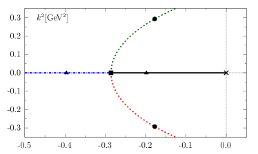
Figure 1: The position of the poles of the quark propagator in the complex $k^{2}$ plane (in GeV²) is shown. Lines represent the position of the pole with varying $m_{d}$: black solid line is the first real-valued solution for $m_{d}<m_{d}^{crit}$, blue dashed-dotted line is second real-value solution for $m_{d}<m_{d}^{crit}$, and red and green dotted lines represent complex conjugated solutions for $m_{d}>m_{d}^{crit}$. The symbols indicate the following solutions: circles represent vacuum value of $m_{d}$, square represent solution for $m_{d}^{crit}$, triangles represent solutions with the property $z_{2}-z_{1}=z_{1}$, which is used as a confinement-deconfinement criterion, and cross represent zero $m_{d}$.

However, the problems are:

1. How to perform analytical continuation of the meson polarization loops integral beyond point $\mathrm{M}_{\mathrm{thr}}$? The prescription for complex-valued poles [6, 7] leads to the suppression of the imaginary part of polarization loops. However, there is a cusp in the real part of the loop at the pinch point, which seems unphysical.

2. What is the physical meaning of the second real-valued solution? It has a wrong sign of residue, which make it similar to Lee-Wick QED model with Pauli-Villars regulator [14]. The first real solution with decreasing of $m_{d}$ goes to zero, meaning the quark becomes a current one, while the second mass in this limit approaches infinity. At $m_{d}^{crit}$ they have the same value.

II.2 Suggestions for remove quark thresholds

There are various methods for removing thresholds:

1. Represent the quark propagator as an entire function in virton model [15] (in Minkowski metric)

   $$\mathrm{S}(p)=-M\exp\biggl{(}-l\hat{p}-p^{2}L^{2}/4\biggr{)},$$ (12)

   where $M$, $l$ and $L$ are some model parameters. Similarly, in the quark confinement model of hadrons [16], the confinement is realized through ansätze for quark propagator averaged in gluon background.

2. IR-cutoff in NJL model with proper time regularization [17] with function

   $$\frac{1}{s+M^{2}}=\int\limits_{0}^{\infty}d\tau\mathrm{e}^{-\tau(s+M^{2})}\quad\to$$ (13)

   $$\to\int\limits_{\tau_{UV}^{2}}^{\tau_{IR}^{2}}d\tau\mathrm{e}^{-\tau(s+M^{2})}=\frac{\mathrm{e}^{-\tau_{UV}(s+M^{2})}-\mathrm{e}^{-\tau_{IR}(s+M^{2})}}{s+M^{2}}$$

   or with three dimensional IR cut-off [18]. The function (13) is quite often used to model confined propagators [19, 20, 21, 22].

3. Scalar (or vector) part of quark propagator as entire function [23]

   $$\mathrm{D}(k^{2})=\frac{1-\exp\left(-{\left(k^{2}+m_{c}^{2}\right)}/{\Lambda^{2}}\right)}{k^{2}+m_{c}^{2}}.$$ (14)

4. Cut in $\alpha$-space [24] of the whole expression for polarization loops. The expression for the polarization loop with quark propagators is represented by the usual prescriptions in $\alpha$-space (Schwinger parameterization). In the integral over the sum of $\alpha$, the upper limit is changed from infinity to $1/\lambda$.

It should be noted that there are two groups of approaches: modifying each propagator [15, 23] or the whole loop integral [16, 17, 18, 24].

In a nonlocal model, the problem with a momentum-dependent mass $m(p^{2})$ is that for gauge invariance, it is necessary to modify the vertices of interaction with external currents, along with the quark propagator. As a result, it is unclear how to implement the modification of the loop integral.

II.3 Confining $\alpha$-prescription for quark propagator

If the scalar propagator has only pole singularities, it can be represented as the sum of its poles

$$\mathrm{D}(k^{2})=\sum\limits_{i=1}^{N}\frac{R_{z_{i}}}{k^{2}+z_{i}}$$ (15)

where $N$ is number of poles (for Gaussian form-factor $N=\infty$). Poles are sorted by the size of the real part of $z_{i}$ with $z_{1}$ having the smallest real part.

Another expansion of the $\mathrm{D}(k^{2})$ is based on its high-energy $k^{2}$ behavior, i.e., expansion over $m_{d}$

$$\mathrm{D}(k^{2})=\frac{1}{k^{2}+m_{c}^{2}}-\frac{2m_{c}m_{d}g(k^{2})}{(k^{2}+m_{c}^{2})^{2}}+O(m_{d}^{2}).$$ (16)

The Laplace transform is defined as:

$$\mathrm{D}(k^{2})=L\left\{\mathbf{D}(\alpha)\right\},\quad\mathrm{D}(k^{2})=\int\limits_{0}^{\infty}d\alpha\mathrm{e}^{-\alpha k^{2}}\mathbf{D}(\alpha).$$ (17)

Series corresponding to the above equations (15) and (16) can be obtained with inverse Laplace transforms $\mathbf{D}(\alpha)=L^{-1}\left\{\mathrm{D}(k^{2})\right\}$ for each term:

$$\mathbf{D}(\alpha) =\sum\limits_{i=1}^{\infty}{R_{z_{i}}}\mathrm{e}^{-\alpha z_{i}},$$ (18)

$$\mathbf{D}(\alpha) =\mathrm{e}^{-\alpha m_{c}^{2}}-2m_{c}m_{d}\mathrm{e}^{-\alpha_{1}m_{c}^{2}}\alpha_{1}\theta(\alpha_{1})+..,$$ (19)

where $\alpha_{i}=\alpha-1/\Lambda^{2i}$. The first series is valid for arbitrary form-factors. In the second one, only the first term is model-independent, and the actual analytical form of the form factor (11) should be used for the other terms. These expansions complement each other, because in order to obtain $\mathbf{D}(0)=1$, an infinite number of terms in series (18) must be summed. In contrast, the first term in series (19) immediately gives the correct answer. On the other hand, in order to obtain the behavior of $\mathbf{D}(\alpha)$ for large $\alpha$, the first terms are sufficient in (18).

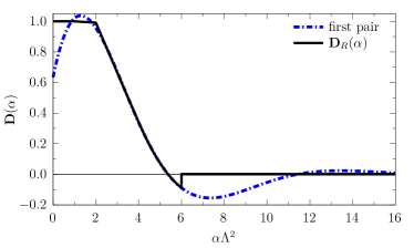
Figure 2: Alpha transformed function $\mathbf{D}(\alpha)$ of scalar propagator: blue dash-dotted line is contribution of first pair of complex-conjugated poles in (18) and solid line is the $\mathbf{D}_{R}(\alpha)$ from (21) with $\Lambda_{c}^{2}=\Lambda^{2}/{6}$.

The region of convergence for the Laplace transform (17) is $k^{2}>-Re(z_{1})$. In order to make this transformation applicable to arbitrary $k^{2}$, it is necessary to change the behavior of the function $\mathbf{D}(\alpha)$ for large values of $\alpha$. The simplest modification is following

$$\mathbf{D}_{R}(\alpha)=\mathbf{D}(\alpha)\theta\bigl{(}{1}/{\Lambda_{c}^{2}}-\alpha\bigr{)}$$ (21)

In this case, the Laplace transformation (17) becomes valid for arbitrary $k^{2}$.

Performing Laplace transform, one can obtain the scalar propagator in momentum space

$$\mathrm{D}_{R}(k^{2}) =\frac{1}{k^{2}+m_{R}^{2}(k^{2})}=$$

$$=\mathrm{D}(k^{2})-\sum\limits_{i=1}^{\infty}\frac{R_{z_{i}}Q\left(k^{2}+z_{i}\right)}{k^{2}+z_{i}},$$ (22)

where $Q(k^{2})=\exp\left(-k^{2}/\Lambda_{c}^{2}\right)$. $\mathrm{D}_{R}(k^{2})$ is entire function, since $Q(0)=1$ and all the singularities have been subtracted. On the other hand, as $k^{2}$ becomes large, $\mathrm{D}_{R}(k^{2})$ tends to $\mathrm{D}(k^{2})$, since $\Lambda_{c}<\Lambda$.

From the equation (22), one can obtain the mass function $m_{R}(k^{2})=\sqrt{\mathrm{D}_{R}^{-1}(k^{2})-k^{2}}$.

The behavior of $\mathbf{D}_{R}(\alpha)$ is shown in Fig.2. The asymptotic behavior of the function $\mathbf{D}(\alpha)$ is determined by its two lowest complex conjugate poles, i.e. $i=1,2$ in (18). As illustrated in the Fig.2 that this mode occurs at $\alpha$ of the order of $3/\Lambda^{2}$.

To calculate the polarization loop in (9), the prescription for propagators with complex masses can be used [6]. The main difference is that, instead of pole singularities, branch cut points will appear in the complex plane. The result of the calculation of the pion polarization loop is presented in Fig. 3. One can observe that the cusp-like behavior of the meson polarization loop around $-1$ GeV² is absent for the $\mathrm{D}_{R}(k^{2})$. The possible choice of $\Lambda_{c}$ is as follows: as mentioned in footnote 6, $\Lambda_{c}<\Lambda$. On the other hand, if $\Lambda_{c}$ is too small, the polarization operator of the pion will grow too much for $-p^{2}>1$ GeV². A value of $\Lambda_{c}=\Lambda/\sqrt{6}$ appears to be a reasonable compromise which leads to a reasonable behavior of $m_{R}(k^{2})$, see footnote 7. This corresponds to a numerical value of $\Lambda_{c}=307$ MeV.

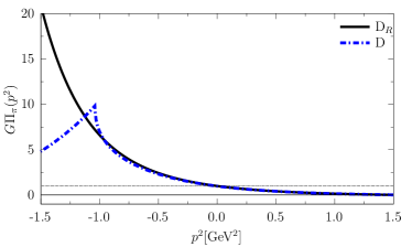
Figure 3: Pion polarization loop times four-quark coupling constant in nonlocal model (blue dash-dotted line) and with confining prescription (black solid line). Thin dashed horizontal line denote $1$ which is correspond to meson pole.

Since quarks can freely propagate in the deconfined phase, a pole for real negative $k^{2}$ should be present. As the poles on the right-hand side of Eq. (22) occur simultaneously in $\mathrm{D}(k^{2})$ and in the second term with sum, it is possible to start the summation at $i=2$. In this case, one can rewrite the expression Eqs.(22) for $\mathrm{D}_{R}(k^{2})$ in the form

$$\mathrm{D}_{R}(k^{2})=\mathrm{D}(k^{2})-\sum\limits_{i=2}^{\infty}\frac{R_{z_{i}}Q\left(k^{2}+z_{i}\right)}{k^{2}+z_{i}}=$$

$$\quad=\frac{R_{z_{1}}}{k^{2}+z_{1}-i\epsilon}+\bigg{[}\mathrm{D}(k^{2})-\frac{R_{z_{1}}}{k^{2}+z_{1}}-$$

$$-\sum\limits_{i=2}^{\infty}\frac{R_{z_{i}}Q\left(k^{2}+z_{i}\right)}{k^{2}+z_{i}}\bigg{]},$$ (23)

where the only pole is isolated and the expression in square brackets is an entire function. In the limit of $m_{d}$ approaching zero, the first pole approaches $z_{1}\to m_{c}^{2}$, with a residue of $R_{z_{1}}\to 1$ , and the expression within the brackets approaches zero.

The two-phase confinement-deconfinement model is:

1. Confined phase: the subtraction sum in Eq.(22) starts from $i=1$. $\mathrm{D}_{R}(k^{2})$ is an entire function.

2. Deconfined phase: the subtraction sum starts from $i=2$. $\mathrm{D}_{R}(k^{2})$ has one pole which corresponds to the pole quark mass.

An important question is about symmetries - what will happen to the gauge symmetry and chiral symmetry? The situation is clearer with gauge symmetry: one simply needs to include $m_{R}(k^{2})$ in the expressions for effective vertices [10] instead of $m(k^{2})$, and the Ward identity is automatically satisfied in this case.

For chiral symmetry, the situation is more complicated. By construction there is a fine-tuning between the gap equation (7) and the pion polarization loop (9) [25] and changing of only the mass due to confinement prescription breaks this fine-tuning. One possible solution is to determine the form factor based on the mass using Eq. (6). Alternatively, one can adjust the normalization of $g(p)$ at the pion vertex. Numerically, these corrections are around two percent for the model parameters used and $\Lambda_{c}^{2}=\Lambda^{2}/6$.

III Finite T behavior

The mean field thermodynamic potential is [26, 27]

$$\Omega^{MF}=\frac{m_{d}^{2}}{2G}-4\sum_{i=0,\pm}\int_{k,n}\ln\bigg{[}k_{n,i}^{2}+m^{2}(k_{n,i}^{2})\bigg{]}+$$

$$+U(\Phi,\bar{\Phi})+\Omega_{0},$$ (24)

where $k_{n,i}=(\omega_{n}^{i}-i{\mu})^{2}+\mathbf{k}^{2}$ and $\int_{k,n}\equiv T\sum_{n}\frac{d^{3}p}{(2\pi)^{3}}$. Fermionic Matsubara frequencies $\omega_{n}^{i}$ are partially shifted due to the presence of a Polyakov loop $\omega_{n}^{\pm}=\omega_{n}\pm\phi_{3}$, $\omega_{n}^{0}=\omega_{n}$ and $\omega_{n}=(2n+1)\pi T$. The thermodynamic potential is divergent due to the current quark contribution. The infinite normalization constant, $\Omega_{0}$, is chosen such that the pressure should be zero under vacuum conditions, which means at zero temperature, zero chemical potential, and for the vacuum $m_{d}$ value.

In the presence of the Polyakov loop, the equations of motion for the mean fields are

$$\frac{\partial\Omega^{MF}}{\partial m_{d}}=0,\quad\frac{\partial\Omega^{MF}}{\partial\phi_{3}}=0.$$ (25)

For comparison, the three models are considered:

1. Nonlocal quark model

2. Confined quark model (the sum in eq. (22) starts from $i=1$)

3. Confinement-deconfinement model (the sum in eq. (22) starts from $i=1$ in confined phase and $i=2$ in deconfined phase.)

The boundary between phases in model (III) is determined by the properties of quark propagator. To a first approximation, in the deconfined phase, there are real solutions to Eq. (1), whereas in the confined phase, only complex-valued solutions are possible. However, it seems that the region where two real poles almost coincide should also be included in the confined phase. In practice, we use a criterion that the difference between the two real poles is of the order of the first one, i.e., in the deconfined phase, $z_{2}-z_{1}>z_{1}$. The corresponding points of $m_{d}$ are approximately 319 MeV, which is the border between real and complex pole solutions, and 310 MeV when $z_{2}-z_{1}>z_{1}$ (the position of the poles is shown in Fig.1).

Since the modification (22) and (23) is $m_{d}$-dependent one should include this behavior when taking the derivatives from the thermodynamic potential (24) in (25). Therefore if one uses the analytical form of thermodynamic potential eq. (24), the expression for the $m_{d}$ gap equation should be changed. Alternatively, one could keep the analytical form of the gap equation

$$\frac{\partial\Omega_{R}}{\partial m_{d}}=\frac{m_{d}}{G}-8\sum_{i=0,\pm}\int_{k,n}g(k_{n,i}^{2})m(k_{n,i}^{2})\mathrm{D}_{R}(k_{n,i}^{2}),$$ (26)

and calculate the thermodynamic potential numerically from gap equation

$$\Omega_{R}=\int\limits_{0}^{m_{d}}dm_{d}\frac{\partial\Omega_{R}}{\partial m_{d}}+C(T,\mu),$$ (27)

using $C(T,\mu)$ as the integration constant. $C(T,\mu)$ is equal to the value of $\Omega^{MF}$, taken at zero $m_{d}$, for a given values of $T$, $\mu$, and $\phi_{3}$ with normalization $\Omega_{R}=0$ in vacuum. It is very instructive to study the $m_{d}$ dependence of the thermodynamic potential in almost vacuum, since there is no influence from the Polyakov loop in this case. In Fig. 4 ${\partial\Omega_{R}}/{\partial m_{d}}$ and $\Omega_{R}$ are shown for models (I)-(III).

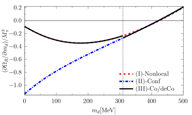
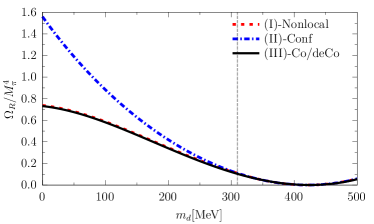
Figure 4: ${\partial\Omega_{R}}/{\partial m_{d}}$ and $\Omega$ in vacuum as a function of $m_{d}$ for three models: red dotted line nonlocal quark model (I), blue dash-dotted line is for confining model (II) and solid line for model with confinement/deconfinement transition (III). Thin vertical line corresponds to confinement/deconfinement border.

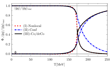
Figure 5: Finite temperature behavior of quark condensate divided to vacuum value (upper curves at left side) and Polyakov loop (downer curves at left side) for three models: red dotted line nonlocal quark model (I), blue dash-dotted line is for confining model (II) and solid line for model with confinement/deconfinement transition (III).

The finite temperature behavior of the quark condensate and the Polyakov loop are shown in Fig. 5. One can see here that even for the confining model (II), the quark condensate (and similarly $m_{d}$) decreases as the temperature increases. The reason for this is the gap equation (26). In the numerator of the integrand, there is a form factor $g(k^{2})$. The Matsubara frequency is proportional to $T$, and the first fermionic frequency is nonzero ($\omega_{0}=\pi T$). Therefore, as the temperature increases, the second term on the right-hand side of (26) becomes strongly suppressed due to the form factor. Therefore, in order to fulfill the gap equation, a corresponding decrease of $m_{d}$ is needed.

The finite $T$ phase transition in model (III) is of first order. This is due to the fact that the gap equations in the two phases are not completely synchronized. Fig. 4 shows that the gap equation (upper part) is not smooth, and there is a jump in the behavior of ${\partial\Omega_{R}}/{\partial m_{d}}$ between the phases. In some conditions, both solutions are possible. However, as can be seen in Fig. 5, the finite $T$ behavior of model (III) is not significantly different from that of the model (I).

At finite chemical potential, the second minimum at low $m_{d}$ appears in models (I) and (III), i.e., in the deconfined phase. At a certain critical value of $m_{d}$, the system undergoes a transition from a confined to a deconfined state. In model (II), this is not the case by design.

IV Conclusions

The paper discusses a simple prescription based on modifying the Laplace transform of the quark propagator in order to phenomenologically model confinement. The main goal of the work is to improve the analytical behaviour of the quark propagator. At finite $T/\mu$, two phases are considered: in the confined phase, the quark propagator does not have pole singularities, and in the deconfined phase, it has a single physical pole. As a result, mean field calculations for the critical temperature and chemical potential in this scheme are almost unchanged. Pole singularities in the complex plane are absent, and therefore there are no physical consequences that can be caused by poles. Instead, the mass function has cuts in the complex plane, and instabilities discussed in [28] are present, although they are less significant.

One can expect that a more interesting situation will arise with $1/N_{c}$ corrections. Namely, the mesonic polarization loops at leading order in the nonlocal model exhibit a cusp-like behavior when poles in the complex plane are located inside the integration contour. For finite temperature and zero chemical potential, one can calculate the mesonic correction to the quark condensate using only the Euclidean properties of the polarization loops. At finite chemical potential, the cusp-like behavior of meson polarization loops can make calculations challenging.

However, our prescription is not free from problems. Some of these problems are technical and can be easily solved. In order for the pion to be massless in the chiral symmetric case, when $m_{c}\to 0$, it is necessary to modify the pion-quark vertex. The value of $g(0)$, which represents the coupling between the pion and quark, should slightly deviate from 1. The first order phase transition at finite T for model (III) with a confinement-deconfinement phase transition occurs because the gap is not a smooth function of $m_{d}$.

The most important conceptual problem is the exponential growing of meson polarization loops in Minkowski space. This issue arises because if the quark propagator has no singularities at finite $p^{2}$, it will have an essential singularity at infinity. How to solve this problem remains unclear, but sub-leading $1/N_{c}$ corrections, such as pion dressing of the quark propagator, may introduce physically motivated singularities. The pion-quark dressing is discussed by V. N. Gribov in his confinement theory [29].

This work is supported by supported by the CAS President’s international fellowship initiative (Grant No. 2023VMA0015); the project of the Ministry of Education and Science of the Russian Federation (”Analytical and numerical methods of mathematical physics in problems of tomography,quantum field theory, fluid and gas mechanics”no. 121041300058-1); the National Natural Science Foundation of China under Grants No. 12375117; and the Youth Innovation Promotion Association of Chinese Academy of Sciences (Grant No. Y2021414).

The authors thank the I.V. Anikin, Yu.M. Bystritskiy, V.P. Lomov and B. Zhang for fruitful comments.

References

- Gasser and Leutwyler [1984] J. Gasser and H. Leutwyler, Annals Phys. 158, 142 (1984).
- Nambu and Jona-Lasinio [1961] Y. Nambu and G. Jona-Lasinio, Phys. Rev. 124, 246 (1961).
- Roberts and Schmidt [2000] C. D. Roberts and S. M. Schmidt, Prog. Part. Nucl. Phys. 45, S1 (2000) .
- Gomez Dumm and Scoccola [2002] D. Gomez Dumm and N. N. Scoccola, Phys. Rev. D 65, 074021 (2002) .
- Dorokhov and Tomio [2000] A. E. Dorokhov and L. Tomio, Phys. Rev. D 62, 014016 (2000).
- Cutkosky et al. [1969] R. E. Cutkosky, P. V. Landshoff, D. I. Olive, and J. C. Polkinghorne, Nucl. Phys. B 12, 281 (1969).
- Bhagwat et al. [2003] M. Bhagwat, M. A. Pichowsky, and P. C. Tandy, Phys. Rev. D 67, 054019 (2003).
- Ratti et al. [2006] C. Ratti, M. A. Thaler, and W. Weise, Phys. Rev. D 73, 014019 (2006).
- Plant and Birse [1998] R. S. Plant and M. C. Birse, Nucl. Phys. A 628, 607 (1998).
- Gomez Dumm et al. [2006] D. Gomez Dumm, A. Grunfeld, and N. Scoccola, Phys. Rev. D 74, 054026 (2006).
- Alkofer et al. [2004] R. Alkofer, W. Detmold, C. S. Fischer, and P. Maris, Phys. Rev. D 70, 014014 (2004).
- Dorkin et al. [2015] S. M. Dorkin, L. P. Kaptari, and B. Kämpfer, Phys. Rev. C 91, 055201 (2015) .
- Windisch [2017] A. Windisch, Phys. Rev. C 95, 045204 (2017) .
- Lee and Wick [1969] T. D. Lee and G. C. Wick, Nucl. Phys. B 9, 209 (1969).
- Dubnickova et al. [1979] A. Z. Dubnickova, G. V. Efimov, and M. A. Ivanov, Fortsch. Phys. 27, 403 (1979).
- Efimov and Ivanov [1993] G. V. Efimov and M. A. Ivanov, The Quark confinement model of hadrons (IOP, Bristol, UK, 1993) p. 177.
- Ebert et al. [1996] D. Ebert, T. Feldmann, and H. Reinhardt, Phys. Lett. B 388, 154 (1996) .
- Blaschke et al. [2001] D. Blaschke, G. Burau, M. K. Volkov, and V. L. Yudichev, Eur. Phys. J. A 11, 319 (2001).
- Gutierrez-Guerrero et al. [2010] L. X. Gutierrez-Guerrero, A. Bashir, I. C. Cloet, and C. D. Roberts, Phys. Rev. C 81, 065202 (2010) .
- Roberts et al. [2010] H. L. L. Roberts, C. D. Roberts, A. Bashir, L. X. Gutierrez-Guerrero, and P. C. Tandy, Phys. Rev. C 82, 065202 (2010), .
- Wang et al. [2013] K.-l. Wang, Y.-x. Liu, L. Chang, C. D. Roberts, and S. M. Schmidt, Phys. Rev. D 87, 074038 (2013) .
- Marquez et al. [2015] F. Marquez, A. Ahmad, M. Buballa, and A. Raya, Phys. Lett. B 747, 529 (2015) .
- Radzhabov and Volkov [2004] A. E. Radzhabov and M. K. Volkov, Eur. Phys. J. A 19, 139 (2004).
- Branz et al. [2010] T. Branz, A. Faessler, T. Gutsche, M. A. Ivanov, J. G. Korner, and V. E. Lyubovitskij, Phys. Rev. D 81, 034010 (2010) .
- Osipov et al. [2007] A. Osipov, A. Radzhabov, and M. Volkov, Phys. Atom. Nucl. 70, 1931 (2007).
- Radzhabov et al. [2011] A. Radzhabov, D. Blaschke, M. Buballa, and M. Volkov, Phys. Rev. D 83, 116004 (2011) .
- Carlomagno and Villafañe [2019] J. P. Carlomagno and M. F. I. Villafañe, Phys. Rev. D 100, 076011 (2019) .
- Benic et al. [2012] S. Benic, D. Blaschke, and M. Buballa, Phys. Rev. D 86, 074002 (2012) .
- Gribov [1999] V. N. Gribov, Eur. Phys. J. C 10, 91 (1999) .