Niels Richard Hansen
Department of Mathematical Sciences, University
of Copenhagen Universitetsparken 5, 2100 Copenhagen Ø, Denmark,
Niels.R.Hansen@math.ku.dk
Abstract.
In this note we show a new version of the trek rule for the
continuous Lyapunov equation. This linear matrix equation characterizes the
cross-sectional steady-state covariance matrix of a Gaussian Markov process,
and the trek rule links the graphical structure of the drift of the
process to the entries of this covariance matrix. In general, the
trek rule is a power series expansion of the covariance matrix, while
for the special case where the drift is acyclic, it simplifies to a
polynomial in the off-diagonal entries of the drift matrix. Using the
trek rule we can give relatively explicit formulas for the entries of
the covariance matrix for some special cases of the drift matrix.
Furthermore, we use the trek rule to derive a new lower bound for the
variances in the acyclic case.
1. Introduction
With any matrix and a
positive semidefinite matrix, we can define a Gaussian Markov process
on as a solution to the stochastic differential equation
(1)
where is a -dimensional Brownian motion, see, e.g.,
Jacobsen (1993) or Section 3.7 in Pavliotis (2014).
We call the
drift matrix and is called the diffusion matrix or the
volatility matrix.
The Markov process has
an invariant distribution if and only if the matrix is stable,
that is, if and only if all eigenvalues of have strictly negative
real part. In this case, the invariant distribution is Gaussian with mean
and covariance matrix , which is the unique
solution to the (continuous) Lyapunov equation
When the process is stationary, that is, when it is started
in its (unique) invariant distribution, the Gaussian distribution
, with solving
(2), is the cross-sectional distribution of
at any time . Questions regarding estimation and identification of and/or
from cross-sectional observations of the process were treated by
Varando & Hansen (2020) and Dettling et al. (2023).
The main contribution of this note is
a novel representation of in terms of the
drift and volatility matrices and . As briefly discussed below,
there are many well known representations of the solution of (2),
but we derive a novel trek rule that links the graphical structure of to the
entries of . For linear structural equation models, such
trek rules are well known and useful, see Sullivant et al. (2010) and
Section 4 in Drton (2018). We show in Section 3
that the new trek rule can
be used to give a lower bound for the variances in the acyclic case.
1.1. The Lyapunov equation
The Lyapunov equation
(2) is a linear matrix equation. Using the kronecker
product, we can rewrite it as
(3)
where is the identity matrix and
denotes the vectorization of the matrix . When is stable,
the matrix is invertible,
and the unique solution to (3) is given by
(4)
The representation (4) shows
that is a rational function of the entries of and ,
but (4) is not very explicit, nor is it efficient for numerical computation
of the solution. There is a vast literature on numerical methods for
solving the Lyapunov equation efficiently, see, e.g., Simoncini (2016)
for a review.
We will not be particularly concerned with numerical
methods in this note, but rather with giving a new representation of
the solution that is interpretable in terms of the graphical structure
of the drift matrix . To this end, we will use the well known
integral representation of the solution given by
(5)
Here, denotes the matrix exponential of , and the
integral is understood as a matrix integral. It is convergent when
is stable. See Varando & Hansen (2020) and the references therein for
further details on the integral representation of the solution.
1.2. Graphs
We will represent the non-zero entries of the
drift matrix and the volatility matrix
by a mixed graph with nodes ,
directed edges, , and blunt edges, .
Definition 1.1.
A pair of matrices is
compatible with a mixed graph if
implies and implies
.
Example 1.2.
We consider the specific model with ,
This pair is compatible with the graph as given by (A) in Figure 1. The eigenvalues of are
with all real parts strictly negative, and is thus stable. Solving the
Lyapunov equation gives the invariant covariance matrix
Figure 1. Mixed graph (A) representing a model with
variables and with a diagonal -matrix.
The edge labels of the directed (blue) edges
are the values of the non-zero entries in the -matrix,
while all the blunt (red) edges correspond to the
diagonal entries of all being .
The mixed graph (B) is the same as (A) but with
all directed self-loops removed. We call (B) the base
graph of (A).
We use standard graph terminology, see, e.g., Maathuis et al. (2019).
Specifically we let a walk be a sequence of (not necessarily unique)
nodes where each node is connected
to the next by an edge. A walk from to is directed if
all edges are directed toward . For example, in Figure 1 (A),
the walk
is a walk from to , and
is a directed walk from to .
A mixed graph is allowed to have self-loops. It will be convenient to
have a version of the graph without directed self-loops, which we call the
base graph.
Definition 1.3.
The base graph of a mixed graph is
obtained from by removing all directed self-loops.
In Figure 1 (B) we have the base graph of the mixed graph (A).
A walk in the base graph is called a base walk. The walk
in 1 (A)
is not a base walk due to the self-loop , while
is a base walk.
2. Treks and trek rules
We define treks for mixed graphs as walks with a specific structure.
Definition 2.1.
A trek in a mixed graph is a walk of the form
(6)
Here and denote the number of nodes to the left
of and to the right of , respectively.
The trek given by (6) is said to be a trek from to .
The pair is the top of the trek,
and if we refer to as the top.
The nodes and are the left-hand
and right-hand sides of the trek, respectively. The top nodes are
connected by a blunt edge, possibly a blunt self-loop, while all other edges are directed.
The left-hand side of the trek forms a directed walk from to with
nodes, and the right-hand side forms a directed walk from to
with . It is possible for a trek to have ,
in which case the trek is just , which is possibly a
blunt self-loop .
Definition 2.2.
Let be compatible with a mixed graph
and let be a trek in with top .
The weight of the trek is the product of the edge weights
along the trek, that is,
The walk
in Figure 1 (A) is an example of a trek from to with top
and with weight .
With the definitions above, we can state the following trek rule
obtained by Varando & Hansen (2020).
Let be compatible with a mixed graph , and let
be stable and be positive semidefinite. Then the solution of the Lyapunov
equation (2) is given by
(7)
where denotes the set of all treks from to
in , and
for any trek and , where .
The representation (7) expresses
in terms of a, possibly infinite, sum of the trek weights over all treks from to ,
but with the weights multiplied by the factor (not depending on and ), and we have to
let outside of the sum. This makes the
representation (7) somewhat clumsy and difficult to use and interpret.
The new trek rule that we give below essentially
interchanges the summation and limit operation by a translation of
by the identity matrix (and by possibly rescaling ).
Throughout we will let
(8)
Since the Lyapunov equation is invariant to rescaling,
we can w.l.o.g. assume that has spectral radius strictly smaller than
when is stable. If not, we can always rescale and to ensure this
without changing .
Proposition 2.4.
Let be compatible with a mixed graph , and let
be stable and be positive semidefinite. When
has spectral radius strictly smaller than , the solution of the Lyapunov
equation (2) is given by
(9)
where denotes the set of all treks from to
in .
Proof.
Using the series expansion of the exponential
function we get
Here we have used the assumption on the spectral radius to justify the
interchange of the integration and summation in the fourth line. The
trek representation follows by taking the -th entry and noting that
is precisely the sum over all trek weights,
,
for treks from to with nodes on the left-hand side and
nodes on the right-hand side.
∎
The trek weights are monomials in the and coefficients,
and (9) provides a (generally infinite) power series representation
of the covariances in terms of these coefficients. Some factors in the monomials
are the diagonal entries , while the remaining
factors are off-diagonal entries of (that coincide
with off-diagonal entries of ) and entries of . It is possible,
as we will show, to derive a trek rule where the contributions from the
the diagonal entries are separated from the off-diagonal entries.
Recall that the base graph of a mixed graph is
obtained by removing all directed self-loops. A base trek is then a trek in
the base graph , and it is a trek without any self-loops. Any
trek in can regarded as a base trek combined with
a total of self-loops on the
left-hand side and self-loops on the
right-hand side. Here and denote the total
number of self-loops for node present in the trek on the left- and
right-hand side, respectively. If node is not present in the left-hand
side of the base trek, say, then . If node is present
once in the left-hand side of the base trek, then denotes the
number of self-loops at that position. If node is present more than once in the
left-hand side of the base trek, then the total number of self-loops
can be distributed in several ways among the different positions
of node .
For a base trek, , in and multiindices
we define
as the number of ways the and self-loops can be positioned
along the trek. If the base trek does not contain repeated nodes in
its left- or right-hand sides, , but
when contains repeated nodes, it is possible that
. Define also
and similarly for .
Definition 2.5.
For and a
base trek define
(10)
It may not be obvious that the series in (10) converges. Its
absolute convergence does, however, follow from Corollary 2.6 below
by taking and letting and
for for a small . Then has spectral radius
strictly smaller than by Perron-Frobenius theory, and
for all base treks
in the complete graph since (12) below is finite and
all terms in that sum are positive.
Corollary 2.6.
Let be compatible with a mixed graph , and let
be stable and be positive semidefinite. If has spectral radius strictly smaller
than and ,
(11)
(12)
where denotes the set of all treks from to
in the base graph of .
Proof.
The formula (11) follows by splitting the sum (9) into
an outer sum over the base treks and an inner sum over self-loops.
Specifically,
Finally, (12) follows by noting that
and that for any base trek .
∎
Note that for a base trek, the monomial
does not depend on the
diagonal elements of , and (12)
provides a certain disentanglement of how the total
covariance depends on the self-loop coefficients
and the other edge coefficients.
3. Acyclic models
If the directed part of the base graph is acyclic,
and thus a DAG, we say that the model given by and is acyclic. Choosing any
topological order of the nodes will make the -matrix lower triangular.
We assume throughout this section that the model is acyclic and that
the nodes are ordered in a topological order such that
is lower triangular, that is,
The diagonal entries of are then the eigenvalues, and is stable
if and only for all . By rescaling, we can assume that
for all so that .
For any acyclic model, we conclude that (12) gives a
representation of . Moreover, since the directed
part of forms a DAG, and there are no loops but
self-loops in , the number of base treks from to is finite
when is triangular, and (11) provides a
finite sum representation of . That is,
the representation (12) is a polynomial in the
off-diagonal entries of and the entries of .
The factors in (12)
depending in the diagonal entries of may also be simplified a bit.
For an acyclic model any base trek has no nodes repeated on either side
(though the
same node can be present once on the left- and once on the right-hand side).
This means that , and if we
define
then
(13)
The expression (13) does not appear to simplify further
in general. However, if all the diagonal entries of are equal, in which case we can
assume them all equal to by rescaling, the trek rule simplifies further.
Figure 2. The mixed graph (A) for a general acyclic model with the nodes in
a topological order, and the mixed graph (B) for the specific model in Example 3.2.
Corollary 3.1.
Let be compatible with a mixed graph , and let
be lower triangular and be positive semidefinite. If
for then the solution of the Lyapunov equation
(2) is given by
(14)
where denotes the set of all treks from to
in the base graph of .
Proof.
First note that when for all ,
the matrix is stable. Moreover, for
, and since
Then and all
other entries of are 0. The only base treks
from to are of the form, for ,
for which , , .
This shows that
(15)
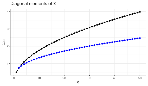
Figure 3 shows the variance as a function of .
It is monotonely increasing. This is not surprising,
since the sink node , in a certain sense, accumulates all the variance from
the other nodes.
Figure 3. The variance in Example 3.2
given by (15) as a function of (black) and the lower bound given by
(19) (blue).
It is well known that for acyclic linear additive noise models,
the variance tends to increase along the topological order of the nodes
if the parameters of the model are all of comparable magnitudes. If that is
the case, it may even be possible to learn the topological order
from the order of the variances (Reisach et al., 2021). Example 3.2
suggests that this may also be the case for acyclic Lyapunov models.
The remaining part of this section is devoted to proving a lower bound
on the variance in terms of the other (co)variances
that sheds some light on this phenomenon.
Recall that , so with
and we have the following identity for the
binomial coefficient
Plugging this into the sum above and using the definition of in (16) gives
∎
Lemma 3.5.
For and we have
(17)
Proof.
Note that , so we may assume that .
Since all terms in the sum defining are non-negative and
we find that
∎
Write the matrices and in block form as
where is a matrix,
and is a -dimensional row vector, and similarly for
.
Proposition 3.6.
Let be a stable lower triangular matrix and a diagonal
positive semidefinite matrix. With the solution of
the Lyapunov equation, the following lower bound holds on the variance
:
(18)
Proof.
The base treks from to are either of the form
or for a
base trek from to with .
Since , we have
the following representation of :
Using the binomial and geometric series, the sum in the first term equals
and plugging this into the sum in the second term gives
Combining these results gives
∎
Example 3.7.
This is a continuation of Example 3.2. We first
derive a slightly different representation of that
is easier to compare to the lower bound in (18).
From (15) we have
The second term above is except from the factors
within the sum. Observe that
with the factor being equal to for . This shows that
To compute the lower bound in (18), we first
note that and , thus
Moreover, , thus . This shows that the lower bound in (18)
is indeed
(19)
as we also found above. The computations in this example show that
we cannot in general replace the factor in the bound by a larger
constant, and certainly not by . The lower bound is shown in Figure
3.
4. Concluding remarks
Trek rules are useful for linking the entries of the solution to the Lyapunov
equation to graphical properties of the underlying mixed graph. An straightforward
observation is that if there is no trek from to .
The general trek rule in Proposition 2.4 is, however, more complicated than
the well known trek rule for linear structural equation models, and even in the
acyclic case it does not simplify to a polynomial representation in general. This is due to the
self-loops. Corollary 3.1 and Example 3.2 shows that
in some special cases a simpler polynomial trek rule is possible for acyclic models.
As an example of a non-trivial application of the trek rule, we derived the
lower bound in Proposition 3.6 on the variance
for a stable acyclic model with a diagonal matrix.
5. Acknowledgements
The trek rules in Proposition 2.4 and Corollary 2.6
were discovered while the author was visiting Mathias Drton at the Technical University of
Munich in November and December 2021. I am grateful to Mathias for hosting me.
More recently, Alexander Reisach mentioned to the author that lower bounds on
the variances in for acyclic models would be of interest, and the trek rule seemed
well suited for this purpose. I am grateful to Alexander for this suggestion.
The author was supported by a research grant (NNF20OC0062897) from Novo Nordisk Fonden.
References
(1)
Dettling et al. (2023)
Dettling, P., Homs, R., Améndola, C., Drton, M. & Hansen, N. R. (2023), ‘Identifiability in continuous Lyapunov models’, SIAM Journal on Matrix Analysis and Applications44(4), 1799–1821.
Drton (2018)
Drton, M. (2018), Algebraic problems in structural equation modeling, in ‘The 50th Anniversary of Gröbner Bases’, Mathematical Society of Japan, Tokyo, Japan, pp. 35–86.
Jacobsen (1993)
Jacobsen, M. (1993), A brief account of the theory of homogeneous Gaussian diffusions in finite dimensions, in Niemi, H. et.al, ed., ‘Frontiers in Pure and Applied Probability’, Vol. 1, pp. 86–94.
Maathuis et al. (2019)
Maathuis, M., Drton, M., Lauritzen, S. & Wainwright, M., eds (2019), Handbook of Graphical Models, Handbooks of Modern Statistical Methods, CRC Press.
Pavliotis (2014)
Pavliotis, G. (2014), Stochastic Processes and Applications: Diffusion Processes, the Fokker-Planck and Langevin Equations, Texts in Applied Mathematics, Springer New York.
Reisach et al. (2021)
Reisach, A. G., Seiler, C. & Weichwald, S. (2021), Beware of the simulated DAG! causal discovery benchmarks may be easy to game, in A. Beygelzimer, Y. Dauphin, P. Liang & J. W. Vaughan, eds, ‘Advances in Neural Information Processing Systems’.
Simoncini (2016)
Simoncini, V. (2016), ‘Computational methods for linear matrix equations’, SIAM Review58(3), 377–441.
Sullivant et al. (2010)
Sullivant, S., Talaska, K. & Draisma, J. (2010), ‘Trek separation for Gaussian graphical models’, Ann. Statist.38(3), 1665–1685.
Varando & Hansen (2020)
Varando, G. & Hansen, N. (2020), Graphical continuous Lyapunov models, in J. Peters & D. Sontag, eds, ‘Proceedings of the 36th Conference on Uncertainty in Artificial Intelligence (UAI)’, Vol. 124 of Proceedings of Machine Learning Research, PMLR, pp. 989–998.