Hopf and Bautin bifurcations in a 3D model for pest leafhopper with stage structure and generalist predatory mite

Abstract.

In a recent paper of Yuan and Zhu (J. Differential Equations 321(2022) 99-129), the nature of dynamics of a generalist predator and prey with stage structure is modeled as a three-dimensional coupled nonlinear differential system. A detailed analysis of the bifurcation shows that the model exhibits a high complexity in its dynamics, which arises from the use of predatory mites as agent for controlling stage structures of tea green leafhopper pest. Unfortunately, there is a mistake in Proposition 2.2, item (3), also the hypothesis in Proposition 3.3 is incorrect. In this paper, we revisit the model and straighten those mentioned errors as in item (3), changed the existing hypothesis by a suitable one and give a corrected proof of Proposition 3.3 in its new form. Also, we show that the model does undergo both Hopf bifurcation and Bautin bifurcation, and numerical examples are given to support the analytic results.

1. Introduction

The production of tea is frequently threatened by one of the most prevalent insect plagues insect plagues in many Asian nations is the tea green leafhopper or Empoasca onukii, and the mite Anystis baccarum has been applied as a plague control agent, which is a predatory that is beneficial to the tea plantations. For the purpose of researching the interactions between adult populations, Yuan and Zhu [5] constructed a three-dimensional ordinary differential equation model, which enables them to use bifurcation theory to investigate the causes and reasons existing behind their complex dynamics. However, in contrast to their earlier paper [4], this takes into account the interaction between generalist predator mite and two different developmental stages of E. onukii.

In [5], the authors consider a model to analyze dynamics and inform biological control. In particular, they perform a bifurcation study of a 3D nonlinear system, and found some complex bifurcation phenomena, such as Bogdanov-Takens bifurcation, Hopf bifurcation, saddle-node bifurcation of codimension 1 and 2, and bifurcations of nilpotent singularities of elliptic and focus type of codimension 3. In addition, they found that all codimension 3 bifurcations in the two-dimensional center manifold of the system are connected by the nilpotent focus of codimension 4, which acts as an organizing center. However, there is a mistake in Proposition 3.3 where the authors assume that $\kappa_{2}<\widehat{\kappa}_{2}$ must be true in order to show that a Hopf bifurcation exists at the coexistence equilibrium points, this hypothesis is incorrect.

Motivated by the aforementioned research, our work is devoted to fix those mentioned gaps and some others errors. According to the known results, the existence of a Bautin bifurcation (generalized Hopf) in the model described by Yuan and Zhu [5] was not supported by any evidence. Thus, in this manuscript we will present numerical data to support the existence of Hopf bifurcation of codimension 1 and 2 (Bautin).

In order to obtain results that, up to this moment, cannot be obtained analytically, as well as to generate phase portraits and bifurcation plots, we heavily rely on advanced continuation and bifurcation techniques implemented in the MatCont software package [1]. Finally, we stress that some calculations were made easier by using the computer algebra system Wolfram Mathematica, version 12.

We want to emphasize how some calculations were made easier by using the computer algebra system.

The paper is organized as follows. In section 2 we introduce the model system. In order to make this work self-contained and facilitate the lecture to the reader, we summarize briefly some current known facts regarding equilibrium points in Section 3. The local analysis of the stability of the interior (coexistence) equilibrium points is provided in Section 4. In Section 5 Hopf bifurcation of the interior equilibrium point of the system is discussed. To illustrate the theoretical findings in, we used phase portraits and numerical bifurcation diagrams that are given in Section 6. Furthermore, we use the numerical software MatCont [1] to compute curves of equilibria and to compute several bifurcation curves. We particularly approximate a family of limit cycles emanating from a Hopf point. Our obtained results give a step forward improving some results given in [5].

2. Mathematical model formulation

In the following, we briefly discuss the underlying model considering the tea plantation that has a designated area for growing tea trees.To introduce the mathematical model, we use $E_{1}$ and $E_{2}$ to represent, respectively, the E. onukii hatchlings (adults and nymphs) as well as eggs at time $t$, while $M(t)$ denotes the A. baccarum. By employing a modeling approach that was used in [4], the model with generalist predator-prey and functional response, Holling type II, also with a prey life cycle stage structure of prey is described by the differential equations system

(1) $$\begin{array}[]{l}\dot{E}_{1}=r_{1}E_{2}-\alpha E_{1},\vspace{0.2cm}\\ \dot{E}_{2}=\alpha E_{1}-\kappa_{1}E_{2}^{2}-\dfrac{mE_{2}M}{a+E_{2}},\vspace{0.2cm}\\ \dot{M}=r_{2}M-\kappa_{2}M^{2}+\dfrac{cmE_{2}M}{a+E_{2}},\end{array}$$

where the dot means derivative with respect to the time $t$. All the parameters are positive and their biological meanings are the following: The rate at whichE. onukii eggs hatch is $\alpha$, $a$ is the number of E. onukii that A. baccarum has managed to locate and successfully capture in an average amount of time, the conversion rate is given by $c$, the maximum number of E. onukii that A. baccarum can sustain during the foraging period is given by $m$, the adult E. onukii rate of oviposition is given by $r_{1}$, and the constant intrinsic growth rate of A. baccarum is indicated by $r_{2}$, $\kappa_{1}$ and $\kappa_{2}$ are the intra-specific levels of competition among adult of E. onukii and A. baccarum, respectively.

It is important to remark that $a>0$ indicates that the predator is generalist and that if it does not exist available prey it has an alternative source of food.

Before beginning our search, we shall reduce the number of parameters in model (1). To do so, firstly, we introduce a change of variables and a time rescaling $(E_{1},E_{2},M,t)\to(aX_{1},aX_{2},acY,\tau)$, given by

$$E_{1}=aX_{1},\quad\qquad E_{2}=aX_{2},\quad\qquad M=acY,\quad\qquad t=\dfrac{1}{cm}\tau.$$

Observe that we still denote $\tau$ by $t$ and we have renamed the variables $(X_{1},X_{2},Y)$ again as $(E_{1},E_{2},M)$ for convenience. Thus, system (1) can be reduced as follows

(2) $$\begin{array}[]{l}\dot{E}_{1}=\hat{r}_{1}E_{2}-\hat{\alpha}E_{1},\vspace{0.2cm}\\ \dot{E}_{2}=\hat{\alpha}E_{1}-\hat{\kappa}_{1}E_{2}^{2}-\dfrac{E_{2}M}{1+E_{2}},\vspace{0.2cm}\\ \dot{M}=\hat{r}_{1}M-\hat{\kappa}_{2}M^{2}+\dfrac{E_{2}M}{1+E2},\end{array}$$

where $\hat{r}_{1}=\frac{r_{1}}{cm}$, $\hat{\alpha}=\frac{\alpha}{cm}$, $\hat{\kappa}_{1}=\frac{a\kappa_{1}}{cm}$, $\hat{\kappa}_{2}=\frac{a\kappa_{2}}{cm}$ and dropping all the hats over the parameters, the system becomes

(3) $$\begin{array}[]{l}\dot{E}_{1}=r_{1}E_{2}-\alpha E_{1},\vspace{0.2cm}\\ \dot{E}_{2}=\alpha E_{1}-\kappa_{1}E_{2}^{2}-\dfrac{E_{2}M}{1+E2},\vspace{0.2cm}\\ \dot{M}=r_{1}M-\kappa_{2}M^{2}+\dfrac{E_{2}M}{1+E_{2}}.\end{array}$$

Hence, this system has only five free parameters, namely $\alpha$, $r_{1}$, $r_{2}$, $\kappa_{1}$, $\kappa_{2}$. These will be used as bifurcation parameters. The reader should be warned that system (3) is topologically equivalent to system (1) except at the singularity $E_{2}=-a$.

3. Existence of equilibria

In this section we will summarize the results on feasible equilibrium points of the model system (3) obtained in [5], where it was shown that model (3) displays up to three coexistence equilibria and three boundary equilibria in the first octant.

In the paragraphs below we summarize the main findings obtained there.

The origin $S_{0}=(0,0,0)$ is always an equilibrium point. Additionally, $S_{10}=(p_{1}K_{1},K_{1},0)$ with $K_{1}=\dfrac{r_{1}}{\kappa_{1}}$ and $p_{1}=\dfrac{r_{1}}{\alpha}$ is a non-negative predator-extinction equilibrium, which refers to the proportion of eggs to newly hatched (nymphs and adults) individuals of the E. onukiiat equilibrium. Similar to this, the pest-free equilibrium $S_{01}=(0,0,K_{2})$ exists with $K_{2}=\dfrac{r_{2}}{\kappa_{2}}$. Here, $K_{1}$ is the maximum capacity for E. onukii (nymphs and adults) without of A. baccarum, while $K_{2}$ is the loading capacity for A. baccarum when E. onukii is not present, for the specific tea plantation. Concerning the possible strictly positive equilibrium points corresponding to points located at the intersection of the nullclines $\dot{E}_{1}=0$, $\dot{E}_{2}=0$ and $\dot{M}=0$ in the first octant of the phase space we have that if these exist, they indicate the coexistence of the three species in equilibrium. This is denoted by $\overline{S}=(\overline{E}_{1},\overline{E}_{2},\overline{M})$. Solving the system of nullclines equations for (3), we get that the intersection points are given by the following curves in the $E_{2}M$ plane:

(4) $$U_{1}(E_{2})=M=\frac{(\alpha E_{1}-\kappa_{1}E_{2}^{2})(a+E_{2})}{mE_{2}},$$

(5) $$U_{2}(E_{2})=M=\frac{1}{\kappa_{2}}\left(r_{2}+\dfrac{cmE_{2}}{a+E2}\right),$$

where $E_{1}=p_{1}E_{2}$. Equating $U_{1}(E_{2})$ and $U_{2}(E_{2})$, after some computations we get that $E_{2}$ is determined by the solution of the equation

(6) $$U(E_{2})=E_{2}^{3}-\left(\dfrac{r_{1}}{\kappa_{1}}-2a\right)E_{2}^{2}+\left(a^{2}-2a\dfrac{r_{1}}{\kappa_{1}}+\dfrac{m(cm+r_{2})}{\kappa_{1}\kappa_{2}}\right)E_{2}+\dfrac{a^{2}r_{1}}{\kappa_{1}\kappa_{2}}\left(\dfrac{mr_{2}}{ar_{1}}-\kappa_{2}\right)=0,$$

which may have up to three positive roots. Therefore, the model system (3) can have maximum three feasible interior equilibrium points. By some trivial computations, we get that $E_{2}=0$ associated with the pest-free equilibrium $S_{01}=(0,0,K_{2})$ is a solution of (6), which requires

(7) $$\kappa_{2}=\overline{\kappa}_{2}=\dfrac{r_{2}m}{r_{1}a}.$$

Due to the difficulty to determine the exact solutions of equation (6), we look closely at the Cardano’s formula for the third degree algebra equation provides a criterion, whether one, two or three real solution of (6) exist. This involves a discriminant whose sign determines the nature of roots. This can be expressed as follows:

$$\Delta_{0}=\Delta_{0}(\kappa_{2})=\dfrac{m^{2}}{\kappa_{1}^{4}\kappa_{2}^{3}}\big{(}a_{2}(\kappa_{1})\kappa_{2}^{2}+a_{1}(\kappa_{1})\kappa_{2}+a_{0}(\kappa_{1})\big{)},$$

where

$$a_{2}(\kappa_{1})=4ac(a\kappa_{1}+r_{1})^{3},$$

$$a_{1}(\kappa_{1})=a^{2}(8c^{2}m^{2}-20cmr_{2}-r_{2}^{2})\kappa_{1}^{2}-2ar_{1}\delta_{1}(10cm+r_{2})\kappa_{1}-r_{1}^{2}\delta_{1}^{2},$$

$$a_{0}(\kappa_{1})=4m\delta_{1}^{3}\kappa_{1},$$

with $\delta_{1}=r_{2}+cm$. In addition, the discriminant with respect to $\kappa_{2}$ associated to the second order polynomial $f(\kappa_{1})=a_{2}(\kappa_{1})\kappa_{2}^{2}+a_{1}(\kappa_{1})\kappa_{2}+a_{0}(\kappa_{1})$ becomes

$$\Delta_{1}(\kappa_{1})=(a\kappa_{1}r_{2}+r_{1}\delta_{1})(r_{1}\delta_{1}-a\kappa_{1}\delta_{2})^{3},$$

with $\delta_{2}=8cm-r_{2}$. Let

$$\kappa_{1}^{*}=\dfrac{r_{1}\delta_{1}}{a\delta_{2}}$$

the unique positive root of $\Delta_{1}(\kappa_{1})=0$. Therefore, when $0<\kappa_{1}<\kappa_{1}^{*}$, $\Delta_{0}(\kappa_{2})=0$ can have two positive roots, denoted by $\kappa_{2}^{-}$ and $\kappa_{2}^{+}$. Furthermore, if $\kappa_{1}^{*}$ into $\Delta_{0}(\kappa_{2})=0$, then one gets

$$\kappa_{2}^{*}=\dfrac{\delta_{1}^{2}\delta_{2}}{27r_{1}ac^{2}m},$$

and follows that $\Delta_{0}(\overline{\kappa}_{2})=0$ at

$$\overline{\kappa}_{1}=\dfrac{r_{1}(r_{2}-cm)}{r_{2}a},\qquad\text{with}\quad{\color[rgb]{1,0,0}r_{2}}>cm.$$

Therefore, we conclude the following result.

Proposition 1 ([5]).

In the $(\kappa_{1},\kappa_{2})$ plane, three curves

$$C_{0}:\kappa_{2} =\overline{\kappa}_{2},\qquad\kappa_{1}>0,$$

$$C_{\triangle}^{-}:\kappa_{2} =\kappa_{2}^{-}(\kappa),\qquad 0<\kappa_{1}<\kappa^{*},\quad\kappa_{2}>0,$$

$$C_{\triangle}^{+}:\kappa_{2} =\kappa_{2}^{+}(\kappa),\qquad 0<\kappa_{1}<\kappa^{*},\quad\kappa_{2}>0,$$

divide the region $\kappa_{1}>0$, $\kappa_{2}>0$ into four subregions $V_{0}$, $V_{1}$, $V_{2}$ y $V_{3}$ (see Figure 1):

$$V_{0} =\{(\kappa_{1},\kappa_{2})\mid\kappa_{1}>0,\quad(\kappa_{2}<\kappa^{-}(\kappa_{1}))\cap(\kappa_{2}<\overline{\kappa}_{2})\},$$

$$V_{1} =\{(\kappa_{1},\kappa_{2})\mid\kappa_{1}>0,\quad\kappa_{2}<\bar{\kappa_{2}}\}\setminus V_{3},$$

$$V_{2} =\{(\kappa_{1},\kappa_{2})\mid\kappa_{1}>0,\quad\kappa_{2}^{-}(\kappa_{1})<\kappa_{2}<\overline{\kappa}_{2}\},$$

$$V_{3} =\{(\kappa_{1},\kappa_{2})\mid 0<\kappa_{1}<\kappa_{1}^{*},\quad\kappa_{2}^{-}(\kappa_{1})<\kappa_{2}<\kappa_{2}^{+}(\kappa_{1})\cap(\kappa_{2}>\overline{\kappa}_{2})\}.$$

1. along $C_{0}$, where $\overline{C}=(\overline{\kappa}_{1},\overline{\kappa}_{2})$

   • if $\kappa_{1}>\overline{\kappa}_{1}$, there is no coexistence equilibria;

   • if $\kappa_{1}=\overline{\kappa}_{1}$, there is a coexistence equilibrium of multiplicity 2, $S_{23}$;

   • if $\kappa_{1}<\overline{\kappa}_{1}$, there are two coexistence equilibria, $S_{2}$ y $S_{3}$.

2. along $C_{\triangle}^{+}$, there is a coexistence equilibrium $S_{3}$ of multiplicity 1 and a coexistence equilibrium of multiplicity 2, $S_{12}$.

3. along $C_{\triangle}^{-}$,

   • if $\kappa_{2}>\overline{\kappa}_{2}$, there is a coexistence equilibrium $S_{1}$ of multiplicity 1 and a coexistence equilibrium of multiplicity 2, $S_{23}$;

   • if $\kappa_{2}\leq\overline{\kappa}_{2}$, there is a coexistence equilibrium of multiplicity 2, $S_{23}$;

4. at $C^{*}(\kappa_{1}^{*},\kappa_{2}^{*})=\left(\frac{r_{1}\delta_{1}}{a\delta_{2}},\frac{\delta_{1}^{2}\delta_{2}}{27r_{1}ac^{2}m}\right)$ there is a coexistence equilibrium point of multiplicity 3, $S_{123}=\left(\frac{r_{1}a\delta_{3}}{\delta_{1}\alpha},\frac{a\delta_{3}}{\delta_{1}},\frac{18r_{1}ac^{2}m}{\delta_{1}\delta_{2}}\right)$ where $0<r_{2}<2cm$.

This allows to split the first quadrant of the positive parameter plane $\kappa_{1}$-$\kappa_{2}$ into four basic regions, labeled $V_{0}$, $V_{1}$, $V_{2}$ and $V_{3}$, where there are 0, 1, 2, and 3 positive equilibrium points, respectively. They are shown in Figure 1. Let $S_{1}$, $S_{2}$ and $S_{3}$ be the three coexistence equilibria, as long as there are exist, where its coordinate $\overline{E}_{2}$ satisfies $\overline{E}_{2}(S_{1})<\overline{E}_{2}(S_{2})<\overline{E}_{2}(S_{3})$. The positive equilibrium where $S_{1}$ and $S_{2}$ coalesce is denoted by $S_{12}$, if it exists. $S_{23}$ and $S_{123}$ may adopt equivalent definitions.

According to the Figure 1, the system (3) there is a chance that the system (3) has a single coexistence equilibrium $S_{1}$ or $S_{3}$, one degenerate coexistence equilibrium $S_{23}$ or $S_{123}$, two coexistence equilibria simultaneously $S_{1}$, $S_{23}$ or $S_{12}$, $S_{3}$ or $S_{2}$, $S_{3}$, or three coexistence equilibria simultaneously $S_{1}$, $S_{2}$, and $S_{3}$.

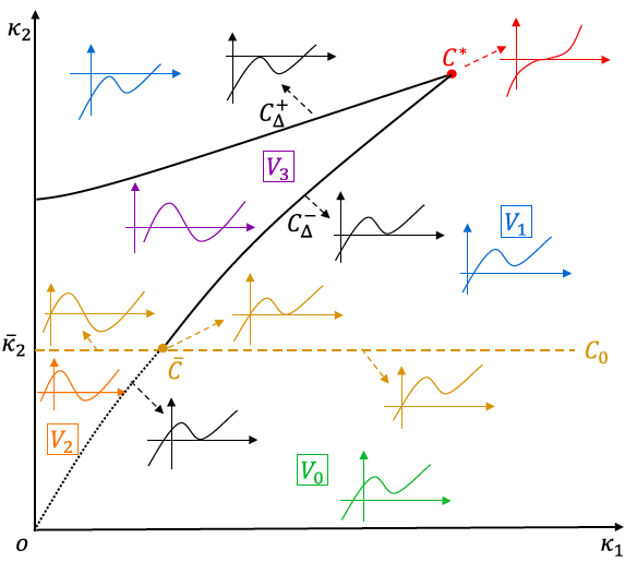
Figure 1. Existence of positive equilibriums (positions and number) for the system (3) with parameters $\kappa_{1}$ and $\kappa_{2}$. The figure was taken from [5].

A schematic diagram with a combined collection of coexistence equilibria and how they are transformed into new ones after some pair of existing or new aquilibria collapse is given in Figure 2.

Figure 2. The diagram shows the bifurcation of coexistence equilibria. The points $S_{1}$ and $S_{2}$ collide when the parameter $\kappa_{2}=\kappa_{2}^{-}(\kappa_{1})$ and the coinciding equilibria is $S_{12}$. In a similar way, the equilibria $S_{2}$ and $S_{3}$ collide when $\kappa_{1}=\overline{\kappa}_{1}$ giving rise to $S_{23}$. If $\kappa_{1}=\kappa_{1}^{*}$ and $\kappa_{2}=\kappa_{2}^{*}$ it occurs that all equilibria collapses, that is, $S_{12}=S_{23}=S_{123}$.

4. Stability analysis of the coexistence equilibria

In this section, we shall discuss the local stability of the model system (3) at the coexistence equilibrium point $\overline{S}$. The Jacobian matrix of system (3) evaluated at $\overline{S}$ has the form

(8) $$J(\overline{S})=\left(\begin{array}[]{ccc}-\alpha&r_{1}&0\\ \alpha&P(\overline{E}_{2})U^{\prime}_{1}(\overline{E}_{2})&-P(\overline{E}_{2})\\ 0&\kappa_{2}\overline{M}U^{\prime}_{2}(\overline{E}_{2})&-\kappa_{2}\overline{M}\end{array}\right),$$

where prime (^′) denotes the derivative with respect to $\overline{E}_{2}$ and $P(\overline{E}_{2})=\dfrac{m\overline{E}_{2}}{a+\overline{E}_{2}}$.

In order to perform an analysis comparative to the one presented in [5], we write the right associated characteristic polynomial of the Jacobian matrix $J(\overline{S})$ as

(9) $$p(\lambda)=-\lambda^{3}-A_{2}\lambda^{2}-A_{1}\lambda-A_{0}$$

where

(10) $$\begin{array}[]{l}A_{2}=\alpha+\kappa_{2}\overline{M}-P(\overline{E}_{2})U^{\prime}_{1}(\overline{E}_{2}),\vspace{0.2cm}\\ A_{1}=\alpha\big{[}\kappa_{2}\overline{M}-P(\overline{E}_{2})U^{\prime}_{1}(\overline{E}_{2})-{\color[rgb]{1,0,0}\bf r_{1}}\big{]}+P(\overline{E}_{2})\kappa_{2}\overline{M}\big{[}U^{\prime}_{2}(\overline{E}_{2})-U^{\prime}_{1}(\overline{E}_{2})\big{]},\vspace{0.2cm}\\ A_{0}=\alpha\kappa_{2}\overline{M}\big{[}P(\overline{E}_{2})\big{(}U^{\prime}_{1}(\overline{E}_{2})-U^{\prime}_{2}(\overline{E}_{2})\big{)}+r_{1}\big{]}.\end{array}$$

By now, the reader should be aware that the expressions $A_{0}$, $A_{1}$ and $A_{2}$ provided above are those that appear in (2.10) of [5], but for computational purposes, we multiply by $-1$ and obtain the following characteristic equation,

(11) $$\lambda^{3}+A_{2}\lambda^{2}+A_{1}\lambda+A_{0}=0.$$

Keep in mind that this polynomial has similar roots and multiplicities as the one given in (9).

In [5], the authors stated that $A_{2}>0$, thus the trace $T(J(\overline{S}))$ of $J(\overline{S})$ satisfies

$$T(J(\overline{S}))=-A_{2}=-\alpha-\kappa_{2}\overline{M}+P(\overline{E}_{2})U^{\prime}_{1}(\overline{E}_{2})<0.$$

As it is well known, the eigenvalue sum is equal to the trace of the matrix, then $J(\overline{S})$ always has at least one eigenvalue that is negative. Additionally, the determinant $D(J(\overline{S}))$ of $J(\overline{S})$ is given by

$$D(J(\overline{S}))=-A_{0}=-\alpha\kappa_{2}\overline{M}\big{[}P(\overline{E}_{2})\big{(}U^{\prime}_{1}(\overline{E}_{2})-U^{\prime}_{2}(\overline{E}_{2})\big{)}+r_{1}\big{]},$$

which is the product of the three eigenvalues. Hence, if $J(\overline{S})$ has one zero eigenvalue, then $D(J(\overline{S}))=0$, leading to $U^{\prime}_{2}(\overline{E}_{2})-U^{\prime}_{1}(\overline{E}_{2})=\dfrac{r_{1}}{P(\overline{E}_{2})}$.

5. Bifurcation analysis

The aim of the section is to discuss the conditions of the Hopf bifurcation in the model system (3). Here, $\alpha$ is taken as the bifurcation parameter.

Let us define $k_{1}=U^{\prime}_{1}(\overline{E}_{2})$, $k_{2}=U^{\prime}_{2}(\overline{E}_{2})$ and $\overline{k}=k_{2}-k_{1}=\dfrac{r_{1}}{P(\overline{E}_{2})}$. The points $\overline{S}=S_{12}$ and $\overline{S}=S_{23}$ nilpotent equilibria, since in these points $D(J(\overline{S}))=0$ with

(12) $$\kappa_{2}=\widetilde{\kappa}_{2}=\dfrac{acm^{2}\overline{E}_{2}}{(a+\overline{E}_{2})^{2}(a+2\overline{E}_{2})(r_{1}-\kappa_{1}\overline{E}_{2})}.$$

Remark 1.

It is worthwhile to point out that the authors in [5] misused the criteria of ${\mathbb{R}}^{2}$ for the existence of bifurcation points, being that (3) is a system in ${\mathbb{R}}^{3}$.

The next proposition summarizes the local stability results and improves the flaws in item (3), Proposition 3.3 from [5].

Proposition 2.

The following statements on coexistence equilibria of (3) hold, when exist.

1. $S_{1}$ and $S_{3}$ are anti-saddle;

2. $S_{2}$ is a hyperbolic saddle;

3. if $J(S_{12(23)})$ has only one eigenvalue zero and all of its eigenvalues are real, and $T(J(S_{12(23)}))\neq 0$, then $S_{12(23)}$ is a saddle-node of codimension 1;

4. if $J(S_{1(3)})$ has one negative eigenvalue and a pair of pure imaginary eigenvalues, then $T(J(S_{1(3)}))<0$ and $D(J(S_{1(3)}))<0$, so that $S_{1(3)}$ exhibits a Hopf bifurcation point;

5. if $J(S_{12(23)})$ has a double zero eigenvalue and $T(J(S_{12(23)}))<0$, then at $S_{12(23)}$ occurs a Bogdanov-Takens bifurcation.

5.1. Hopf bifurcation at $S_{1}$ or $S_{3}$

To apply the Hopf bifurcation theorem, we must first determine the parameter values at which a pair of complex-conjugate eigenvalues of $J(S_{1(3)})$ cross, in a transversal manner, the imaginary axis of the complex plane while the other eigenvalue remains real and negative.

From Proposition 2, we know that system (3) may exhibit Hopf bifurcation at $S_{1}$ or $S_{3}$, when exists, that is, if $T(J(S_{1(3)}))=-A_{2}<0$ and $D(J(S_{1(3)}))=-A_{0}<0$. These conditions mean that $A_{2}>0$ and $A_{0}>0$.

For what follows in the rest of this paper, we will assume that the characteristic equation (9) of the system (3) has a pair of purely imaginary roots and one real negative root. Therefore, the cubic equation can be factored as

(13) $$(\lambda+A_{2})(\lambda^{2}+A_{1})=0,$$

imposing the usual condition for coefficients

(14) $$A_{0}=A_{1}A_{2},\qquad A_{1}>0.$$

Now, we choose the parameters $\alpha$ as the bifurcation parameter, and fix the other parameters at suitable values. By doing so, we define the function

(15) $$H(\alpha)=A_{0}-A_{1}A_{2}=h_{2}\alpha^{2}+h_{1}\alpha+h_{0},$$

where

$$h_{0} =-\frac{\delta_{1}\overline{E}_{2}+ar_{2}}{\kappa_{2}(a+\overline{E}_{2})^{5}}\bigg{[}2\kappa_{1}\overline{E}_{2}^{2}+(a\kappa_{1}+\delta_{1}-r_{1})\overline{E}_{2}+ar_{2}\bigg{]}$$

$$\qquad\bigg{[}2\kappa_{1}\kappa_{2}\overline{E}_{2}^{4}+(5a\kappa_{1}\kappa_{2}-r_{1}\kappa_{2})\overline{E}_{2}^{3}+2a\kappa_{2}(2a\kappa_{1}-r_{1})\overline{E}_{2}^{2}+a\big{(}cm^{2}-ar_{1}+a^{2}\kappa_{1}\kappa_{2}\big{)}\overline{E}_{2}\bigg{]},$$

$$h_{1} =\frac{1}{(a+\overline{E}_{2})^{2}}\bigg{[}-4\kappa_{1}^{2}\overline{E}_{2}^{4}+\big{[}(6r_{1}-4\delta_{1})\kappa_{1}-4a\kappa_{1}^{2}\big{]}\overline{E}_{2}^{3}$$

$$\qquad-\big{[}a^{2}\kappa_{1}^{2}+a\kappa_{1}(2cm-5r_{1}+6r_{2})+2r_{1}(r_{1}-\delta_{1})+\delta^{2}\big{]}\overline{E}_{2}^{2}$$

$$\qquad+\big{[}(r_{1}-2r_{2})a^{2}\kappa_{1}-a(2r_{2}\delta_{1}-2r_{1}r_{2}+r_{1}^{2})\big{]}\overline{E}_{2}-a^{2}r_{2}^{2}\bigg{]},$$

$$h_{2} =\frac{-2\kappa_{1}\overline{E}_{2}^{2}+(-a\kappa_{1}-\delta_{1}+2r_{1})\overline{E}_{2}+a(r_{1}-r_{2})}{a+\overline{E}_{2}}.$$

Clearly, condition (14) is fulfilled when $H(\alpha)=0$. In fact, the discriminant of the quadratic polynomial in the variable $\alpha$ is given by

$$\Delta_{h} =h^{2}_{1}-4h_{0}h_{2}$$

$$=\frac{1}{(a+\overline{E}_{2})^{4}}\Big{[}4\kappa_{1}^{2}\overline{E}_{2}^{4}+\big{(}4a\kappa_{1}^{2}+4\delta_{1}\kappa_{1}-6r_{1}\kappa_{1}\big{)}\overline{E}_{2}^{3}$$

$$\qquad+\big{[}\delta_{1}^{2}+2a\kappa_{1}\delta_{1}-2r_{1}\delta_{1}+(r_{1}-a\kappa_{1})^{2}-a(3r_{1}-4r_{2})\kappa_{1}+r_{1}^{2}\big{]}\overline{E}_{2}^{2}$$

$$\qquad+a\big{[}r_{1}^{2}-2r_{1}r_{2}+2r_{2}\delta_{1}-ar_{1}\kappa_{1}+2ar_{2}\kappa_{1}\big{]}\overline{E}_{2}+a^{2}r_{2}^{2}\Big{)}$$

$$\qquad-\frac{4\overline{E}_{2}(\delta_{1}\overline{E}_{2}+ar_{2})}{(a+\overline{E}_{2})^{6}\kappa_{2}}\Big{[}\big{(}2\kappa_{1}\overline{E}_{2}+a\kappa_{1}+\delta_{1}-2r_{1}\big{)}\overline{E}_{2}+a(r_{2}-r_{1})\Big{]}$$

$$\qquad\Big{[}\big{(}2\kappa_{1}\overline{E}_{2}+a\kappa_{1}+\delta_{1}-r_{1}\big{)}\overline{E}_{2}+ar_{2}\Big{]}\Big{[}(\overline{E}_{2}+a)^{2}\big{(}(a+2\overline{E}_{2})\kappa_{1}-r_{1}\big{)}\kappa_{2}+acm^{2}\Big{]}.$$

By using the quadratic formula, we can see that the roots of $H(\alpha)=0$ yield

$$\alpha^{-}=\frac{-h_{1}-\sqrt{\Delta_{h}}}{2h_{2}},\qquad\alpha^{+}=\frac{-h_{1}+\sqrt{\Delta_{h}}}{2h_{2}}.$$

Now, we remark that if condition $\Delta_{h}=0$ holds, then there is only one real root for $H(\alpha)=0$. This reads

$$\alpha^{*}=-\frac{h_{1}}{2h_{2}}= \frac{1}{2(a+\overline{E}_{2})\big{(}\overline{E}_{2}\kappa_{1}(a+2\overline{E}_{2})+(\delta_{1}-2r_{1})\overline{E}_{2}+ar_{2}-ar_{1}\big{)}}$$

$$\qquad\Big{[}-4\kappa_{1}^{2}\overline{E}_{2}^{4}-2\kappa_{1}\big{(}2a\kappa_{1}+\delta_{1}-3r_{1}\big{)}\overline{E}_{2}^{3}$$

$$\qquad-\big{(}a^{2}\kappa_{1}^{2}+a(2cm-5r_{1}+6r_{2})+2r_{1}(\delta_{1}+r_{1})+\delta_{1}^{2}\big{)}\overline{E}_{2}^{2}$$

$$\qquad+a\big{(}-r_{1}^{2}+r_{1}(2r_{2}+a\kappa_{1})-2r_{2}(a\kappa_{1}+\delta_{1})\big{)}\overline{E}_{2}-a^{2}r_{2}^{2})\Big{]}.$$

Let us turn our attention to determine whether $A_{1}>0$ occurs. We calculated this by using Mathematica software and found that this happens when

$$r_{1}>\dfrac{(a+E_{2})(cmE_{2}+(a+E_{2})r_{2})\alpha}{cmE_{2}^{2}+(a+E_{2})(a\alpha+E_{2}(r_{2}+2\alpha))},$$

$$0<\kappa_{1}<\dfrac{cmE_{2}\big{[}E_{2}(r_{1}-\alpha)-a\alpha\big{]}+(a+E_{2})\big{[}a(r_{1}-r_{2})\alpha-r_{2}\alpha E_{2}+E_{2}r_{1}(r_{2}+2\alpha)\big{]}}{E_{2}(a+2E_{2})\big{[}cmE_{2}+(a+E_{2})(r_{2}+\alpha)\big{]}},$$

and $\widehat{\kappa}_{2}<\kappa_{2}$, with

$$\widehat{\kappa}_{2}=\frac{-acm^{2}\overline{E}_{2}(\delta_{1}\overline{E}_{2}+ar_{2})}{(a+\overline{E}_{2})^{2}(\widetilde{q}_{3}\overline{E}_{2}^{3}+\widetilde{q}_{2}\overline{E}_{2}^{2}+\widetilde{q}_{1}\overline{E}_{2}+\widetilde{q}_{0})},$$

$$\widetilde{q}_{3} =2\kappa_{1}(\delta_{1}+\alpha),$$

$$\widetilde{q}_{2} =a\kappa_{1}\big{(}cm+3\alpha+3r_{2}\big{)}-2\alpha r_{1}+\delta_{1}(\alpha-r_{1}),$$

$$\widetilde{q}_{1} =a\big{(}a\kappa_{1}(r_{2}+\alpha)+(cm-3r_{1}+2r_{2})\alpha-r_{1}r_{2}\big{)},$$

$$\widetilde{q}_{0} =a^{2}\alpha(r_{2}-r_{1}).$$

Remark 2.

We would like to point out that after double-checking the results, we discovered that $\widetilde{q}_{2}$, $\widetilde{q}_{1}$ and $\widetilde{q}_{0}$ expressions obtained are different from those in [5] on page 112. Also, in Proposition 3.3 of [5], the authors failed to make the assumption that $\kappa_{2}<\widehat{\kappa}_{2}$. This claim will be supported in Section 6, where some numerical simulations of the system (3) for various parameter values will demonstrate the formation of limit cycles via Hopf bifurcations in equilibrium, but using the proper inequality $\widehat{\kappa}_{2}<\kappa_{2}$.

Let us assume that $\hat{\lambda}_{1}$, $\hat{\lambda}_{2}$, $\hat{\lambda}_{3}$ are the eigenvalues of (8), or equivalently, the roots of equation (13). Thus, there exists an eigenvalue of (9), say $\hat{\lambda}_{1}$, such that $\hat{\lambda}_{3}=\overline{\hat{\lambda}}_{1}$, and the other eigenvalue satisfies $\hat{\lambda}_{2}<0$. Consequently, $\hat{\lambda}_{2}+\hat{\lambda}_{3}=-A_{2}-\hat{\lambda}_{1}$. As $\hat{\lambda}_{1}$ and $\hat{\lambda}_{3}$ are complex conjugates, it follows that $2\gamma=-A_{2}-\hat{\lambda}_{1}$, where $\gamma$ is the real part of $\hat{\lambda}_{1}$ and $\hat{\lambda}_{3}$.

To assure the occurrence of the Hopf bifurcation we need to guarantee the transversality condition of the Hopf bifurcation theorem. By using (14) we have $2\gamma=-\dfrac{A_{0}}{A_{1}}-\hat{\lambda}_{1}$, and so $\gamma=-\dfrac{1}{2}\left(\frac{A_{0}}{A_{1}}+\hat{\lambda}_{1}\right)$. Differentiating this equation with respect to $\alpha$, and arranging the terms, one reaches

$$\dfrac{\partial\gamma}{\partial\alpha}\bigg{|}_{\alpha=\alpha^{\pm}}=\dfrac{\overline{E}_{2}(\delta_{1}\overline{E}_{2}+r_{2}a)^{2}\Big{[}\kappa_{2}(a+\overline{E}_{2})^{2}(-r_{1}+(a+2\overline{E}_{2})\kappa_{1}+acm^{2})\Big{]}\Big{[}(a+\overline{E}_{2})^{2}(a+2\overline{E}_{2})(-r_{1}+\overline{E}_{2}\kappa_{1})\kappa_{2}+acm^{2}\overline{E}_{2}\Big{]}}{\Big{[}(\overline{q}_{3}\overline{E}_{2}^{3}+\overline{q}_{2}\overline{E}_{2}^{2}+\overline{q}_{1}\overline{E}_{2}+\overline{q}_{0})(a+\overline{E}_{2})^{2}\kappa_{2}+acm^{2}(\delta_{1}\overline{E}_{2}+r_{2}a)\overline{E}_{2}\Big{]}^{2}}$$

where

$$\overline{q}_{3}=2(\alpha^{\pm}+\delta_{1})\kappa_{1},$$

$$\overline{q}_{2}=(3a\kappa_{1}+\delta_{1})\alpha^{\pm}+a\kappa_{1}(3r_{2}+cm)-r_{1}\delta_{1},$$

$$\overline{q}_{1}=a(cm+r_{1}+2r_{2}+a\kappa_{1})\alpha^{\pm}+ar_{2}(-r_{1}+a\kappa_{1}),$$

$$\overline{q}_{0}=a^{2}(r_{2}+r_{1})\alpha^{\pm}.$$

After some algebraic computations, we get that $\dfrac{\partial\gamma}{\partial\alpha}\bigg{|}_{\alpha=\alpha^{\pm}}=0$ if and only if

(16) $$acm^{2}\overline{E}_{2}+(a+\overline{E}_{2})^{2}(a+2\overline{E}_{2})(-r_{1}+\kappa_{1}\overline{E}_{2})\kappa_{2}=0,$$

or

(17) $$acm^{2}+(a+\overline{E}_{2})^{2}(-r_{1}+(a+2\overline{E}_{2})\kappa_{1})\kappa_{2}=0.$$

Through an immediate calculation, from (16) we obtain that

$$\kappa_{2}=\dfrac{acm^{2}\overline{E}_{2}}{(a+\overline{E}_{2})^{2}(a+2\overline{E}_{2})(r_{1}-\kappa_{1}\overline{E}_{2})},$$

that is, $\kappa_{2}=\widetilde{\kappa}_{2}$ where $D(J(\overline{S}))=0$ for $\overline{S}=S_{12}$ or $\overline{S}=S_{23}$. On the other hand, the equation (17) is true for

(18) $$\kappa_{2}=\dfrac{acm^{2}}{(a+\overline{E}_{2})^{2}(r_{1}-a\kappa_{1}-2\kappa_{1}\overline{E}_{2})}.$$

A straightforward computation shows that the equilibrium $\overline{S}=S_{123}$ exists if equalities $U(E_{2})=0$, $\dfrac{dU}{dE_{2}}=0$ and $\dfrac{d^{2}U}{dE_{2}^{2}}=0$ are fulfilled simultaneously, yielding

$$E_{2}^{*}=a\left(-1+\dfrac{3cm}{\delta_{1}}\right),\qquad\kappa_{1}=\kappa_{1}^{*}=\dfrac{r_{1}\delta_{1}}{a\delta_{2}},\qquad\kappa_{2}=\kappa_{2}^{*}=\dfrac{\delta_{1}^{2}\delta_{2}}{27ac^{2}mr_{1}}.$$

Now, after substituting $\overline{E}_{2}=E_{2}^{*}$ and $\kappa_{1}=\kappa_{1}^{*}$ into (18) we get that $\kappa_{2}=\kappa_{2}^{*}$. So, (18) is associated with $\overline{S}=S_{123}$. Therefore, $\dfrac{\partial\gamma}{\partial\alpha}\Big{|}_{\alpha=\alpha^{\pm}}\neq 0$ and the condition of transversality is verified. Hence, the system (3) exhibits a Hopf bifurcation at $\alpha^{\pm}$.

Remark 3.

We observe that the factor

$$acm^{2}\overline{E}_{2}+(a+\overline{E}_{2})^{2}(a+2\overline{E}_{2})(-r_{1}+\kappa_{1}\overline{E}_{2})\kappa_{2}$$

is missing in the algebraic expression of $\dfrac{\partial\gamma}{\partial\alpha}\Big{|}_{\alpha=\alpha^{\pm}}$ given in [5]. Nevertheless, the authors claim that $\dfrac{\partial\gamma}{\partial\alpha}\Big{|}_{\alpha=\alpha^{\pm}}=0$ if only if

$$r_{1}=\kappa_{1}(a+2\overline{E}_{2})+\dfrac{acm^{2}}{(a+\overline{E}_{2})^{2}\kappa_{2}},$$

equivalently to (17), occurs only for points $\overline{S}=S_{12}$ or $\overline{S}=S_{23}$ or $\overline{S}=S_{123}$. The authors are incorrect in their assertion because this value of $r_{1}$ only appears in $\overline{S}=S_{123}$ and not in $\overline{S}=S_{12}$ or $\overline{S}=S_{23}$.

As a result, we have proved the following theorem, which outlines the conditions that are necessary for a Hopf bifurcation to occur.

Theorem 1.

For the set of differential equations (1), if $\widehat{\kappa}_{2}<\kappa_{2}$ and the coexistence point $S_{1}$ or $S_{3}$ exists, then

1. if $\alpha=\alpha^{-}$, or $\alpha=\alpha^{+}$, system (1) goes through a Hopf bifurcation;

2. if $\alpha=\alpha^{*}$, system (1) goes through a Hopf bifurcation, which can be degenerate.

In the next section we provide numerical examples to highlight the existing Hopf bifurcation of codimension 1 and 2.

6. Numerical experiments

In this section we illustrate the creation of limit cycles emanating from the Hopf bifurcations at the equilibrium.

We would like to point out that the reader should be aware that the main purpose of the examples provided is not to discover some new interesting bifurcation behaviors, but rather to demonstrate the validity of our version of Theorem 1, which corrects what is stablished in Proposition 3.3 in [5].

The bifurcation analysis is done using MatCont [1]. This is a package for numerical continuation that runs in a Matlab environment. This numerical simulation tool can also be used to determine the first ($\ell_{1}$) and second ($\ell_{2}$) Lyapunov coefficients by applying the formulae proposed by Kuznetsov in [2].

For the purpose of this section, we consider a case that looks slightly simpler case than the general case, where $a=c=m=1$, which implies that systems (1) and (2) are the same. Biologically this means that the number of removal of adult individuals born from E. onukii attacked by one A. baccarum is equal to $\dfrac{E_{2}M}{1+E_{2}}$. Notwithstanding the system still exhibits very complex dynamics even under this restriction.

In Figure 3 we see the continuation of the equilibrium curve detected with MatCont in the $(\kappa_{1},M)$-plane. During the bifurcation analysis some parameters are fixed at $r_{1}=1.6$, $r_{2}=60$, $\alpha=51.57$ and $\kappa_{2}=0.026927991$ because for this values most types of activity can be seen. The branch of Hopf bifurcations is continued in two parameters $(\kappa_{1},\kappa_{2})$, and a generalized Hopf (GH) point is located. Switching from one branch of equilibria to another branch of equilibria.

And then, one has to note that the bifurcations and related dynamics, including Hopf (H and GH) and Bogdanov-Takens (BT) bifurcations, which reveals the complex dynamics behaviors and the reason behind the complexity of the model (1).

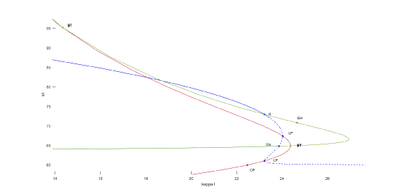
Figure 3. This plot shows the continuation of the equilibrium curve detected with MatCont in the $(\kappa_{1},M)$-plane where the parameter values $r_{1}=1.6$, $r_{2}=60$, $\alpha=51.57$ and $\kappa_{2}=0.026671$ stand fixed: switching from one branch of equilibria to the other and finding two branch points on the other branch. BT, LP, SN, H, CP and GH denote Bogdanov-Takens bifurcation point, limit point, saddle-node point, Hopf bifurcation point, cusp point and degenerate Hopf bifurcation point, respectively. The blue solid and dashed lines represent the stable and unstable hopf bifurcation, respectively.

6.1. Hopf bifurcation

• The system (1) goes through a Hopf bifurcation at the equilibrium point $\overline{S}$, whose coordinates are

  $$(\overline{E}_{1},\overline{E}_{2},\overline{M})=(0.614426554662767,0.528099623732648,72.9478611523887),$$

  and parameter values $\alpha=51.57$, $\kappa_{1}=23.2197961461739$, $\kappa_{2}=0.026671$ $r_{1}=60$ and $r_{2}=1.6$. The eigenvalues of the Jacobian matrix (8) evaluated at $\overline{S}$ are given by

  $$\lambda_{1}=-109.28094024998,\quad\lambda_{2}=1.09824705073231i,\quad\lambda_{3}=-1.09824705073231i.$$

  Moreover, $\widehat{\kappa}_{2}=0.0000801963<\kappa_{2}=0.026671$, so the hypothesis of Theorem 1 holds.

  The first Lyapunov coefficient, obtained by using the software MatCont corresponds to $\ell_{1}=0.02036690>0$. Its positivy means that the Hopf bifurcation is subcritical, namely, the limit cycle arising near equilibrium point is unstable. As indicated in Figure 4, the equilibrium point is stable for $\kappa_{1}<23.2197961461739$, afterwards loses stability at the Hopf (H) bifurcation point, and then degenerates into instability.

  We plot the phase portrait in Figure 5, where the subcritical Hopf bifurcation takes place, an unstable limit cycle (LPC, colored red) mount from the unstable equilibrium.

  

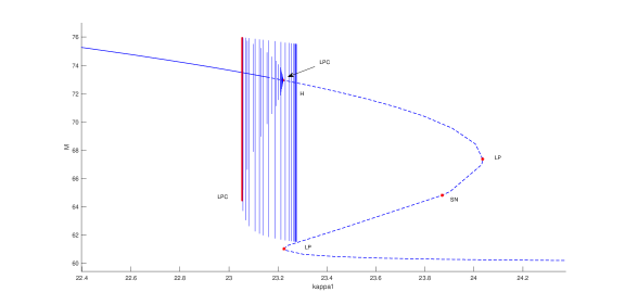
  Figure 4. Diagram of numerical continuation of subcritical Hopf (H) point in the $(\kappa_{1},M)$-plane. The stability of the equilibrium point changes from the stable (solid line) to the unstable (dashed line). This behavior corresponds to the subcritical Hopf bifurcation.

  

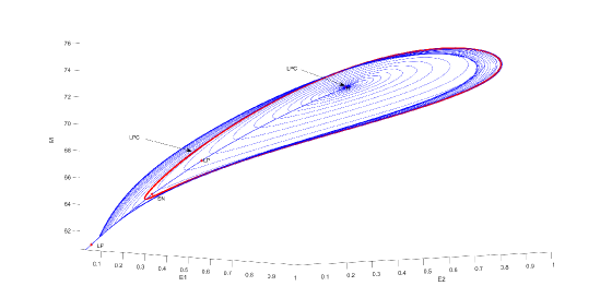
  Figure 5. $(E_{1},E_{2},M)$-phase space. Shown an unstable limit cycle (LPC) solution of system (1) obtained using MatCont by continuation of the orbit emerging from subcritical Hopf (H) point $(\overline{E}_{1},\overline{E}_{2},\overline{M})=(0.614426554662767,0.528099623732648,72.9478611523887)$.

• The model (1) undergoes a subcritical Hopf bifurcation at

  $$(\overline{E}_{1},\overline{E}_{2},\overline{M})=(0.702380773962441,0.418254438462965,73.7892484519822)$$

  for $m=1$, $a=1$, $r_{1}=62.27545$, $r_{2}=1.6$, $\kappa_{1}=24.5$, $\kappa_{2}=0.02568$, $\alpha=37.083850149878$,

  Since $\widehat{\kappa}_{2}=0.000113965<\kappa_{2}=0.02568$, as a result, Theorem 1 is true. Given that $\ell_{1}=0.004838562$, this implies that the bifurcating limit cycle is unstable. Figure 6 displays the phase portrait for this situation.

  

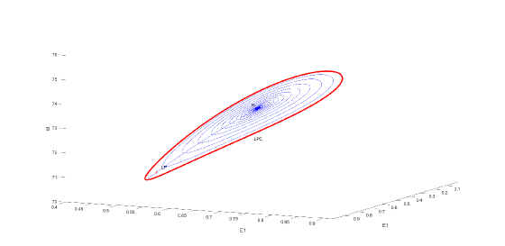
  Figure 6. In the $(E_{1},E_{2},M)$-phase space, it is shown an unstable limit cycle (LPC) solution of the system emerging from subcritical Hopf (H) point $(\overline{E}_{1},\overline{E}_{2},\overline{M})=(0.702380773962441,0.418254438462965,73.7892484519822)$.

6.2. Bautin bifurcation

An important factor in understanding a dynamical system’s overall behavior is the presence of a codimension-2 bifurcation point, which has a significant impact on the qualitative behavior of the system. Here, we perform a bifurcation analysis of Bautin or degenerate codimension-2 Hopf bifurcation at which a fold limit cycle and a Hopf bifurcations occur together.

The numerical simulation tool MatCont indicates that a Bautin point takes place at

$$(\alpha,\kappa_{1},\kappa_{2},r_{1},r_{2})=(53.1351,24.665343,0.026927991,60,1.6).$$

As required by the Theorem 1, it is true $\widehat{\kappa}_{2}=0.0000847597<\kappa_{2}=0.026927991$. For the chosen parameters in Figure 7, a 2D figure in the $(\kappa_{1},M)$-plane displaying the periodic orbits that emerge from the generalized Hopf.

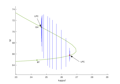
Figure 7. Diagram of numerical continuation of generalized Hopf (GH) point in the $(\kappa_{1},M)$-plane showing the periodic orbits that emerge from such point, when $r_{1}=60$, $r_{2}=1.6$, $\alpha=51.57$ $\kappa_{2}=0.026671$. BT is Bogdanov-Takens point and LPC is limit point of cycle.

The first Lyapunov coefficient $\ell_{1}$ shrinks to zero, which means that the Hopf bifurcation of

$$(\overline{E}_{1},\overline{E}_{2},\overline{M})=(0.51386752,0.44166914,70.794719)$$

degenerates [3], at which, the eigenvalues are given by

$$\lambda_{1}=-109.326162726243,\quad\lambda_{2}=1.0910208605339i,\quad\lambda_{3}=-1.0910208605339i.$$

In order to see if this point is a Bautin bifurcation or has a higher order degeneracy, we need to calculate the second Lyapunov coefficient $\ell_{2}$ with $\kappa_{1}$ and $\kappa_{2}$ as unfolding parameters. With the help of MatCont we obtain that $\ell_{2}=-0.001914430\neq 0$. In Figure 8 the result of the bifurcation analysis is shown. Notice that LPC point (which correspond to the collapse of stable-unstable limit cycles) and Bautin (generalized Hopf, GH) bifurcation point are labeled.

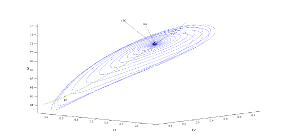
(a) Phase portrait exhibiting Bautin point of codimension 2.

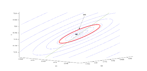
(b) Small limit cycle bifurcating from the generalized Hopf point. Zoom plot of (a).

Figure 8. $(E_{1},E_{2},M)$-phase space. The generalized Hopf bifurcation point is indicated by GH, while the limit point of cycle (labeled by LPC) is a fold bifurcation of the cycle.

6.3. Degenerate Hopf bifurcation with four limit cycles

We provide one example to illustrate the existence of four limit cycles that bifurcate from a degenerate Hopf bifurcation for parameter values close to the focus equilibrium point.

The system (1) has an equilibrium at

$$(\overline{E}_{1},\overline{E}_{2},\overline{M})=(0.667957076496141,0.37421233014172,72.9092840794877)$$

corresponding to $m=1$, $a=1$, $r_{1}=62.27545$, $r_{2}=1.6$, $\kappa_{1}=24.638748097512$, $\kappa_{2}=0.02568$, and $\alpha=34.888830547725$, with eigenvalues

$$\lambda_{1}=-93.80919627015,\quad\lambda_{2}=0.519624557163896i,\quad\lambda_{3}=-0.519624557163896i.$$

Since $\widehat{\kappa}_{2}=0.000117406<\kappa_{2}=0.02568$, then the numerical results agree quite well with the analytical ones for the existence of a Hopf bifurcation.

The numerical results provided by MatCont says that the corresponding first Lyapunov coefficients $\ell_{1}$ becomes zero. This implies that the Hopf bifurcation is degenerate [3], but the critical second Lyapunov coefficient is different from zero, namely $\ell_{2}=0.001968325$. By choosing the parameters $\alpha$ and $\kappa_{1}$ the fold limit cycle codimension-2 Hopf bifurcation occurs at

$$(\alpha,\kappa_{1})=(34.332136490836,24.806008381396).$$

The projection of Hopf bifurcation regions on the $(E_{2},\alpha)$-plane is shown in Figure 9, in which $\ell_{1}=0$ and $\ell_{2}$ are the projection of Bautin bifurcation lines. The bifurcation portrait and the corresponding phase portraits is shown in Figure 9, where it is seen that the degeneracy gives rise to limit folding cycles (LPCs) that surround the equilibrium point.

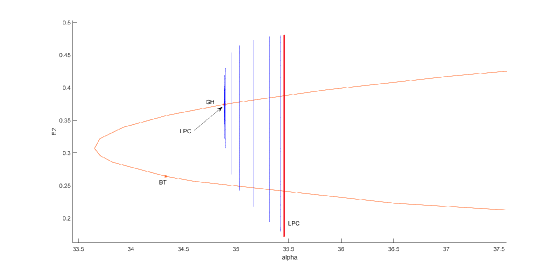
Figure 9. Bifurcation diagram in $(\alpha,E_{2})$-plane with $r_{1}=62.27545$, $r_{2}=1.6$, $\kappa_{1}=24.638748097512$, $\kappa_{2}=0.02568$.

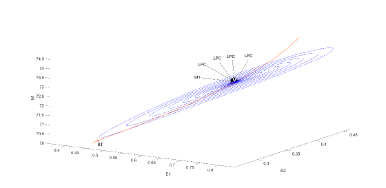
(a) Phase portrait exhibiting Bautin point of codimension 2 for parameter values close to the nilpotent singularity’s focus of codimension 3.

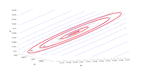
(b) Phase portraits near the Hopf bifurcation of codimension 2. Four small limit cycle bifurcating from the Hopf point. Zoom plot of (a).

Figure 10. In the $(E_{1},E_{2},M)$-phase space. We show a codimension 2-Hopf bifurcation of system (1). The generalized Hopf bifurcation point is indicated by GH and the small four limit point of cycle are labeled by LPC.

References

• [1] W. Govaerts, Y. A. Kuznetsov, and A. Dhooge. Numerical continuation of bifurcations of limit cycles in MATLAB. SIAM J. Sci. Comput., 27(1):231–252, 2005.
• [2] Y. A. Kuznetsov. Elements of applied bifurcation theory, volume 112 of Applied Mathematical Sciences. Springer, Cham, 2023. Fourth edition [of 1344214].
• [3] L. Perko. Differential equations and dynamical systems, volume 7 of Texts in Applied Mathematics. Springer-Verlag, New York, 1991.
• [4] P. Yuan, L.-L. Chen, M. You, and H. Zhu. Dynamics complexity of generalist predatory mite and the leafhopper pest in tea plantations. J. Dynam. Differential Equations, 10 2021.
• [5] P. Yuan and H. Zhu. The nilpotent bifurcations in a model for generalist predatory mite and pest leafhopper with stage structure. J. Differential Equations, 321:99–129, 2022.