KPF Confirms a Polar Orbit for KELT-18 b
Abstract
We present the first spectroscopic transit results from the newly commissioned Keck Planet Finder on the Keck-I telescope at W. M. Keck Observatory. We observed a transit of KELT-18 b, an inflated ultra-hot Jupiter orbiting a hot star ( K) with a binary stellar companion. By modeling the perturbation to the measured cross correlation functions using the Reloaded Rossiter-McLaughlin technique, we derived a sky projected obliquity of ( for isotropic ). The data are consistent with an extreme stellar differential rotation (), though a more likely explanation is moderate center-to-limb variations of the emergent stellar spectrum. We see additional evidence for the latter from line widths increasing towards the limb. Using loose constraints on the stellar rotation period from observed variability in the available TESS photometry, we were able to constrain the stellar inclination and thus the true 3D stellar obliquity to . KELT-18 b could have obtained its polar orbit through high-eccentricity migration initiated by Kozai-Lidov oscillations induced by the binary stellar companion KELT-18 B, as the two likely have a large mutual inclination as evidenced by Gaia astrometry. KELT-18 b adds another data point to the growing population of close-in polar planets, particularly around hot stars.
1 Introduction
KELT-18 b is an ultra-hot Jupiter discovered by the KELT transit survey (McLeod et al., 2017). The planet orbits its F5 type ( K) host star every 2.87 days. Hot stars ( K) with hot Jupiters (HJs) have been observed to have a broad range of obliquities, where the obliquity is defined as the angle between the host star’s rotation axis and the planet’s orbital plane. Conversely, HJs orbiting cooler stars ( K) tend to be aligned with their host star’s rotation axis (Winn et al., 2010; Schlaufman, 2010; Albrecht et al., 2022a). The transition temperature is near the Kraft Break (Kraft, 1967), suggesting realignment mechanisms that are effective for cooler stars–which have convective envelopes and strong magnetic fields–but are ineffective for hotter stars–which have radiative envelopes and weak magnetic fields (Albrecht et al., 2012; Dawson, 2014).
While it is still an unsolved problem, the origins of HJs are likely a combination of multiple formation channels (see Dawson & Johnson 2018 for a review), namely in-situ formation, disk migration, and high eccentricity migration (HEM). HEM likely plays a significant role in shaping the overall HJ population (Rice et al., 2022) but must be triggered by an additional body in the system. This could be another planet, in the case of planet-planet scattering (Rasio & Ford, 1996) or von-Zeipel-Kozai-Lidov111See Ito & Ohtsuka (2019) for a historical monograph. oscillations (ZKL; von Zeipel, 1910; Kozai, 1962; Lidov, 1962) induced by an outer planetary (Naoz et al., 2011; Teyssandier et al., 2013) or stellar companion (Fabrycky & Tremaine, 2007). In the HEM scenario, the HJ originally formed beyond the water ice-line (2 AU) where giant planet formation is efficient (Pollack et al., 1996). The orbital eccentricity was increased through interactions with a perturbing companion until the planet’s periastron distance became small enough for tides to dissipate energy and transfer orbital angular momentum to the star, causing the orbit to shrink and circularize. Either this HEM process, or perhaps a primordial misalignment of the protoplanetary disk (Batygin, 2012), leaves the HJ on an orbit that may be tilted by a large angle relative to the stellar equatorial plane. Only the HJs around stars cooler than the Kraft Break were then able to realign their host star’s rotation axis.
The spin-orbit angle is usually measured as projected on the plane of the sky (), but for systems in which the inclination of the host star’s rotation axis () can be inferred, the true 3D obliquity can be derived (). Recently, Albrecht et al. (2022b) noted that hot Jupiters around hot stars do not span the full range of , but instead show a preference for near polar orbits (–). However, there are still too few systems to be sure that the obliquity distribution has a peak near (Siegel et al., 2023; Dong & Foreman-Mackey, 2023). If there is a “polar peak” it would have important theoretical implications on plausible HJ formation mechanisms, which predict different obliquity distributions (see Albrecht et al., 2022a). For small planets with massive outer companions, secular resonance crossing in the disk dispersal stage may produce polar orbits (Petrovich et al., 2020). For giant planets, an initially inclined orbit inherited from a torqued protoplanetary disk in the presence of a binary companion can give the necessary starting point for subsequent ZKL-driven migration to create a polar HJ (Vick et al., 2023).
The most commonly employed method for measuring the projected obliquity of a star with a transiting planet is to obtain high-resolution spectra throughout a transit and model the Rossiter-McLaughlin effect (Rossiter, 1924; McLaughlin, 1924), which results from the planet’s obscuration of part of the rotating stellar photosphere. This effect is often modeled as an anomalous radial velocity (RV) signal, but measuring precise RVs for hot stars can often be challenging due to their fast rotation rates. The projected equatorial rotation velocity, , broadens (and blends) spectral lines, diminishing the Doppler information content (Bouchy et al., 2001). As a result, stars with km s-1 are usually not amenable to anomalous-RV modeling. However, these fast rotating stars lend themselves to more detailed and direct methods of measuring the stellar obliquity. The Reloaded RM (RRM) method, developed by Cegla et al. (2016), directly models the distortion of the line profile by the transiting planet. By subtracting an out-of-transit reference CCF (representing the star alone) from each in-transit CCF (corresponding to the stellar line profile integrated over the full disk, minus the integrated line profile from within the patch of the star beneath the planet’s shadow), the resulting signal represents the “local” CCF, i.e., the spectrum originating from the portion of the star obscured by the transiting exoplanet (CCF). The RRM method is also sensitive to stellar differential rotation, should the planet be highly misaligned so that it transits a wide range of stellar latitudes (Roguet-Kern et al., 2022).
In this paper we report our derivation of the obliquity of the host star in the KELT-18 system based on a time series of spectra taken during a transit of KELT-18 b with the Keck Planet Finder (KPF). By modeling the spectra according to the RRM method, we found the orbit of KELT-18 b to be nearly perpendicular to the star’s equatorial plane. In Section 2 we derive stellar properties, reexamine the rotation period with TESS photometry, and identify the nearby star KELT-18 B as a bound companion. We describe the Keck Planet Finder and our observations in Section 3, the RRM modeling procedure in Section 4, and dynamical implications for the KELT-18 system in Section 5.
2 KELT-18 System
| Parameter | Value | Unit | Source |
|---|---|---|---|
| KELT-18 | |||
| K | M17 | ||
| M⊙ | M17 | ||
| R⊙ | M17 | ||
| M17 | |||
| M17 | |||
| RV | km s-1 | This work | |
| KELT-18 b | |||
| days | I22 | ||
| JD | I22 | ||
| M17 | |||
| degrees | M17 | ||
| M17 | |||
| M17 | |||
| M17 | |||
| MJ | M17 | ||
| KELT-18 B | |||
| K | M17 | ||
| M⊙ | B22 | ||
| sep | 1082 | AU | B22 |
| mas yr-1 | B22 | ||
| mas yr-1 | B22 | ||
| parallax | mas | B22 | |
| G | mag | B22 | |
| 4.83 | — | B22 |
KELT-18 is a rapidly rotating F4 V star with one known transiting exoplanet, discovered by McLeod et al. (2017) (hereafter M17), and a stellar neighbor. M17 derived robust stellar properties using high resolution spectra, SED fitting, photometry, and evolutionary modeling in a global fit with their transit model. We adopted their best-fit stellar and transit parameters for our analyses herein, with two distinctions noted below. Table 1 lists the full set of adopted parameters.
For the transit midpoint and orbital period of KELT-18 b, we adopted the improved ephemeris of Ivshina & Winn (2022) which implies an uncertainty of only 20 sec in the predicted transit midpoint on the night of our spectroscopic observations (Section 3).
For the projected stellar rotation velocity , M17 noted that their value of km s-1 obtained from a TRES (Szentgyorgyi & Furész, 2007) spectrum is likely an overestimate as the method they used conflates macroturbulence and rotation. M17 also measured a value of km s-1 using a HIRES (Vogt et al., 1994) spectrum and the SpecMatch-Synthetic (Petigura, 2015) framework, but did not adopt this value because the best-fit was outside the range 4800–6500 K over which the code had been calibrated. Since then, the SpecMatch-Emperical (Yee et al., 2017) tool was developed to derive stellar properties for a wider range of effective temperatures (3000–7000 K) by interpolating a grid of library spectra obtained with Keck/HIRES. We ran the same HIRES spectrum obtained by M17 through SpecMatch-Emperical to obtain new estimates of , Fe/H, and . The resulting K is cooler than the K value of M17 and is within the SpecMatch-Synthetic regime. We therefore ran SpecMatch-Synthetic on the same HIRES spectrum and found K and km s-1. Thus, the true value of is likely in the 9–12 km s-1 range. All this together informs our adoption of an informed prior on of km s-1 for our spectroscopic transit analysis in Section 4.
2.1 Stellar rotation period
A significant peak at 0.707 days was observed in the Lomb-Scargle periodogram of the KELT photometry, which M17 interpreted as the rotation period of KELT-18. Given the measured stellar radius, this implied an equatorial rotational velocity of km s-1. While large, it is not atypical for stars of KELT-18’s and to have rotation speeds on the order of km s-1. Combining this with their measured of km s-1, McLeod et al. 2017 noted that the star must have an inclination of . In other words, we are observing KELT-18 nearly pole-on. Since the planet’s orbit is viewed at high inclination, the implication was that the planet’s orbit is nearly polar.
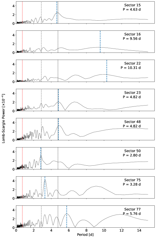
Since the rotation signal in the KELT photometry appeared small compared to the measurement noise, we downloaded the available TESS photometry for KELT-18 to search for variability. KELT-18 was observed by TESS as TIC 293687315 (TOI-1300) in sectors 15, 16, 22, 23, 48, 50, 75, and 77. We downloaded the 1800 s cadence data for sectors 48 and 50, 120 s data for sector 75 and 77, and the 600 s data for the other sectors. We selected data processed by the TESS Science Processing Operations Center pipeline (Caldwell et al., 2020), removed flagged values, stitched the six sectors together, and binned to a common 1 hour cadence using lightkurve (Lightkurve Collaboration et al., 2018). The resulting light curve is shown in Figure 1 along with its Lomb-Scargle periodogram.
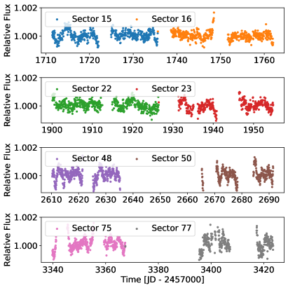
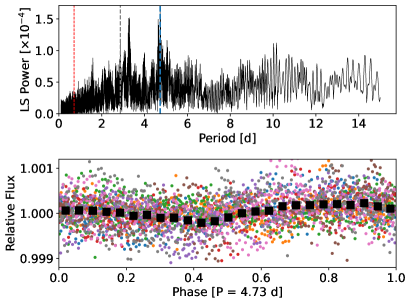
The TESS periodogram does not contain any significant peaks below 3 days. There is a clustering of peaks around 5 days with a maximum power at 4.76 d, and variability on this timescale is visible by eye in the TESS photometry. Stars with KELT-18’s tend to have rotation rates d at (Bouma et al., 2023), so a 5 day rotation period would be reasonable. However, further inspection at the per-sector level (see Appendix A) reveals that this 5 day periodicity is only dominant in sectors 15, 23, and 48. Other sectors show muted variability or strong peaks at other periods. Interactions between multiple spot groups, and/or the presence of differential rotation, can yield multiple periodogram peaks which may further wander in time (Blunt et al., 2023). Altogether, a precise and robust value for the stellar rotation period is not well-determined by the TESS photometry, though it does bring the previous value of 0.707 days into question.
A rotation period of 4.76 days would imply an equatorial rotation speed of km s-1. Given our spectroscopic measurement of is only km s-1, it remains likely that KELT-18 is viewed at low inclination. Conservatively, we adopt a uniform d prior on the rotation period based on the empirical boundary defined by Bouma et al. 2023 and the TESS photometry showing variability on the order of several days. Using the methodology of (Masuda & Winn, 2020), this loose constraint translates into a stellar inclination of .
2.2 KELT-18 B: Neighbor or Companion?
M17 noted a stellar neighbor at 3”.43 separation from KELT-18 B. The neighbor is fainter at . Under the assumption that the neighbor is at the same distance as KELT-18, M17 obtained K. The available astrometry were not precise enough to identify the neighbor as comoving based on its proper motion, though the relatively small sky density of stars in the field around KELT-18 (at high galactic latitude) makes a chance alignment at such a small angular separation unlikely (3).
KELT-18 and KELT-18 B appear in the catalog of stellar companions to TESS Objects of Interest of Behmard et al. (2022) (B22). B22 applied the methodology of Oh et al. (2017) to the Gaia DR3 astrometry (Gaia Collaboration et al., 2023) to determine the likelihood the two stars are comoving. The method propagates the astrometric uncertainties from Gaia into a likelihood ratio comparing the comoving hypothesis () to the null (not comoving) hypothesis (). B22 added a jitter term to account for any unknown systematic effects to improve the reliability of this hypothesis testing. B22 computed for KELT-18 and KELT-18 B, giving strong evidence for the comoving hypothesis. They computed a stellar mass for KELT-18 B of using isoclassify (Huber et al., 2017) and the Gaia magnitudes, in agreement with the estimate from M17. Given the consistent parallaxes ( mas for the primary and mas for the secondary), B22 computed a binary separation from the Gaia astrometry of 1082 AU. The relative velocity vector in the sky plane is thus km s-1. For reference, if both stars were orbiting in the sky-plane on circular orbits, their relative velocity would be 1.8 km s-1. So, unless the two stars have a significant relative radial velocity (which Gaia did not measure), they are likely bound.
3 Observations
We observed a transit of KELT-18 b on UT May 22, 2023 with the Keck Planet Finder (KPF; Gibson et al., 2016, 2018, 2020). KPF is a newly commissioned, optical (445–870 nm), high-resolution (), fiber-fed, ultra-stabilized radial velocity system on the Keck I telescope at W. M. Keck Observatory. Our observations began 25 min before transit ingress and continued until 2 hours after transit egress, only being interrupted by hourly calibration exposures (described below) and a 20 min window near transit egress during which issues with the tip/tilt system prevented precise fiber positioning on the stellar PSF.
We chose a fixed 600 sec exposure time to balance averaging over p-mode oscillations (14 min from the scaling relations of Brown et al. 1991; Kjeldsen & Bedding 1995) with temporal resolution of the transit, while reaching a spectral signal-to-noise ratio (S/N) of at least 100 (typical values were in the green channel and in the red). The KPF “SKY” fiber collected background sky contamination from a position offset several arcsec from KELT-18. We simultaneously acquired broadband Fabry-Pérot etalon spectra in the “CAL” fiber to track instrumental drift, and periodically (once per hour) took a single internal frame with etalon light in the “SKY”, “CAL”, and science fibers as an additional sanity check on drift. We observed a stable linear drift as traced by the simultaneous etalon spectra of m s-1 per hour in the green channel and m s-1 per hour in the red channel. This was well-matched by the hourly all-etalon RVs across each fiber. As a result, we drift-corrected our stellar spectra by Doppler-shifting the derived CCFs by estimated drift using our linear fit to the simultaneous etalon RVs.
We independently extracted 1D stellar spectra from each of the three science “slices” using the public KPF data reduction pipeline (DRP)222https://github.com/Keck-DataReductionPipelines/KPF-Pipeline/. Wavelength calibration was performed for each spectral order using a state-of-the-art laser frequency comb (for nm) and a ThAr lamp (for nm) using calibration frames taken during the standard KPF calibration sequences performed that day. We used the F9 ESPRESSO mask (e.g. Pepe et al., 2002) to derive cross-correlation functions (CCF; Baranne et al., 1996) for each spectral order. This dataset was obtained before a significant charge transfer inefficiency (CTI) in one of the green CCD amplifiers was diagnosed using solar data (Rubenzahl et al., 2023). Because of this, the green CCD readout utilized the original four-amplifier scheme and was thus affected by significant CTI. We masked the flux corresponding to the quadrant of the raw 2D image read by the affected amplifier when deriving CCFs. This affects half of the bluest 20 orders (roughly 445–530 nm). Fortunately, about 78% of the affected wavelengths also appear in the “good” amplifier of the subsequent order, so much of the spectral information is still contained in the final 1D spectrum. The CCFs from each slice were combined in a weighted sum, taking the weights to be proportional to the total flux in each slice from a representative high S/N spectrum. We repeated the same process across all orders, and then again across the green and red CCDs to obtain the final CCF for each observation. We also calculated the unweighted summed CCF to derive photon-noise uncertainties, which we scaled by the relative total flux in the weighted vs. unweighted CCF to yield appropriate uncertainties in each CCF.
We independently verified the systemic velocity reported by M17. We measured this by fitting the CCF of each of the three science traces, for each out-of-transit spectrum. The result was km s-1, in agreement with km s-1 from M17. We found a slightly smaller value of km s-1 by comparing the HIRES spectra used in Section 2 to a telluric model (Kolbl et al., 2015). Gaia (Gaia Collaboration et al., 2023) reports a smaller but less certain km s-1 for KELT-18. We adopt the km s-1 value from our KPF spectra for our analysis.
4 Obliquity of KELT-18 b
4.1 Reloaded Rossiter-McLaughlin Modeling
To measure the obliquity of KELT-18 b, we applied the Reloaded Rossiter-McLaughlin technique (Cegla et al., 2016) to our KPF spectra. We breifly summarize the process here.
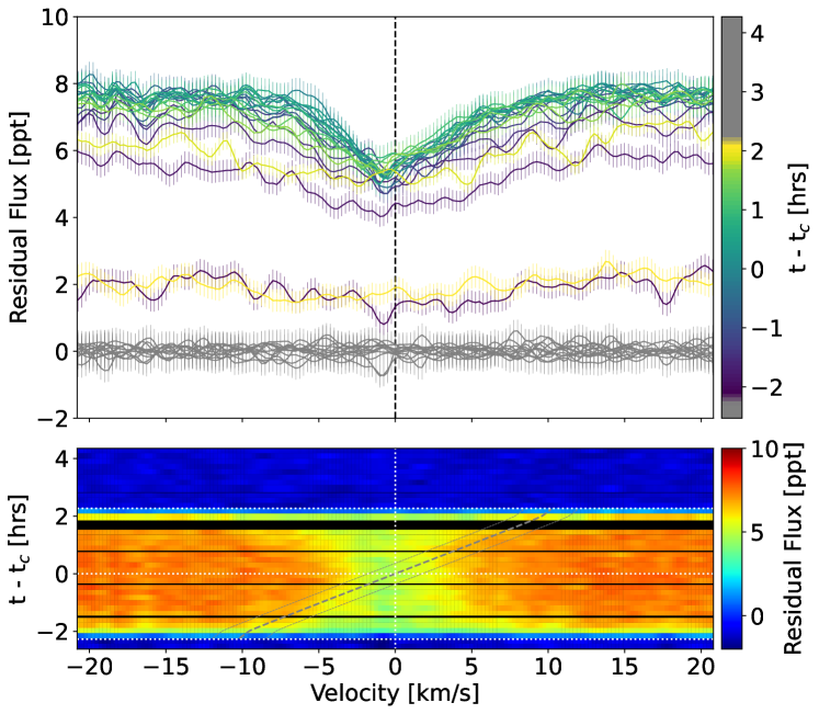
First, we transformed into the stellar rest frame by Doppler shifting the CCFs by our measured systemic velocity and by the expected Keplerian RV induced by KELT-18 b’s orbital motion (using the planet’s mass from M17). The aligned CCFs were then normalized to a continuum value of 1. We then created a stellar template, CCF, by averaging the out-of-transit normalized CCFs. CCF describes the unperturbed average stellar line profile of KELT-18. To isolate the shadow of KELT-18 b, we subtracted each in-transit observation (CCF) from the template to obtain the local line profile within the planet’s shadow, CCFCCFCCF. Since we normalized the CCFs, we multiplied each CCF by the calculated flux at that time according to a white-light synthetic transit light curve model, integrated over the exposure time of each observation. This placed each CCF on the appropriate flux scale.
The resulting CCF time series is shown in Figure 2. Each CCF is fit with a Gaussian profile using curve_fit from scipy (Virtanen et al., 2020), where the continuum, amplitude (i.e., depth), width, and centroid are free parameters. The centroid corresponds to the flux-weighted integrated stellar velocity profile within the shadow of the transiting planet; i.e., the local RV. The local RV is modelled by Eq. 9 in (Cegla et al., 2016),
| (1) |
where is the limb-darkened intensity, the integral is over the patch of star within the planet shadow, and is the stellar velocity field
| (2) |
where is the relative differential rotation rate (the difference in rotation rates at the poles compared to the equator, divided by the equatorial rotation rate). For the Sun, . We used the same coordinate definitions for as in Cegla et al. (2016), but we adapted the implementation of the integral for improved resolution. Instead of defining a Cartesian grid of points centered on the planet’s shadow spanning to and only keeping the points in the grid which satisfied , we generated a “grid” of points according to the sunflower pattern,
| (3) | |||
where is the golden ratio. The result is a set of points uniformly spaced over a circle of radius unity. The points can then be scaled to and centered at the position of the planet to quickly obtain a densely packed grid of points for which each point represents the same projected area of the stellar photosphere. The improved resolution of this grid at the shadow and disk limbs helped to reduce artifacts during ingress/egress, and greatly boosted performance when simulating full line profiles for stars with surface inhomogeneities (Rubenzahl, 2024) .
To fit the local RVs, we modified the radvel package (Fulton et al., 2018) to accept a new function that computes Eq. 1 for each observation. The radvel framework automatically enabled us to perform maximum a-posteriori (MAP) fitting, MCMC sampling using emcee (Foreman-Mackey et al., 2013), and model comparison with the BIC and AIC. We tested several different models: solid body (SB) rotation vs. differential rotation (DR), and with/without center-to-limb variations (CLVs); see Doyle et al. (2023) for more details. The former is a matter of fixing to zero (SB) or letting it float (DR), while the latter requires adding an additional term to Eq. 1 of the form
| (4) |
This polynomial in the intensity-weighted center-to-limb position is a good model for the velocity field introduced by granulation, which is azimuthally symmetric around the disk and varies with center-to-limb position as the line-of-sight intersects the tops of granules at disk-center and the sides of granules at the limb (Cegla et al., 2016). Since CCF has the out-of-transit template subtracted, the net convective blueshift integrated across the full stellar disk has also been removed from the data. Consequently, must be constrained according to Eq. 13 in Cegla et al. (2016). The additional model parameters are thus for a linear () CLV and for a quadratic () CLV.
4.2 MCMC Sampling
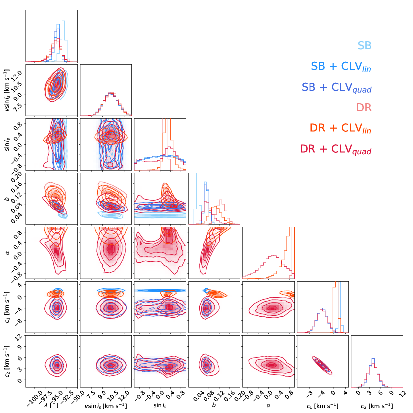
We tested a suite of models within the RRM framework corresponding to each combination of SB or DR, and no CLV, linear CLV (CLV), and quadratic CLV (CLV). The free parameters in all models were the sky-projected obliquity , the projected rotational velocity , the sine of the stellar inclination , and the impact parameter . Models with DR include the degree of differential rotation , and models with CLVs include either (linear) or and (quadratic). We allowed for anti-solar differential rotation by permitting to be negative, with a uniform prior over .
To improve the sampling efficiency, we make the change of coordinates for our fitting basis into a polar coordinate system with as the azimuthal angle and as the radial dimension. The parameters for the fit are thus , , , , , and the CLV coefficients.
Because of the suspected polar orientation of the transit chord, we placed an informed Gaussian prior on of km s-1 based on our analysis of the spectroscopic (Section 2). We also found that this prior, in conjunction with a prior on based on previous transit fits (Table 1), was necessary to discourage the sampler from wandering to solutions of extremely low (1 km s-1) with (unrealistic) grazing transits. The final distributions for were unaffected by the exact boundaries chosen for these priors. We note that Maciejewski (2020) found values of () and () that were significantly discrepant with those measured by M17. We tried setting a prior on to this value and found the MCMC to both not converge and produce a bimodal posterior around 2 km s-1, which is highly inconsistent with the observed width of lines in the KPF spectra and the HIRES, TRES, and APF spectra of M17.
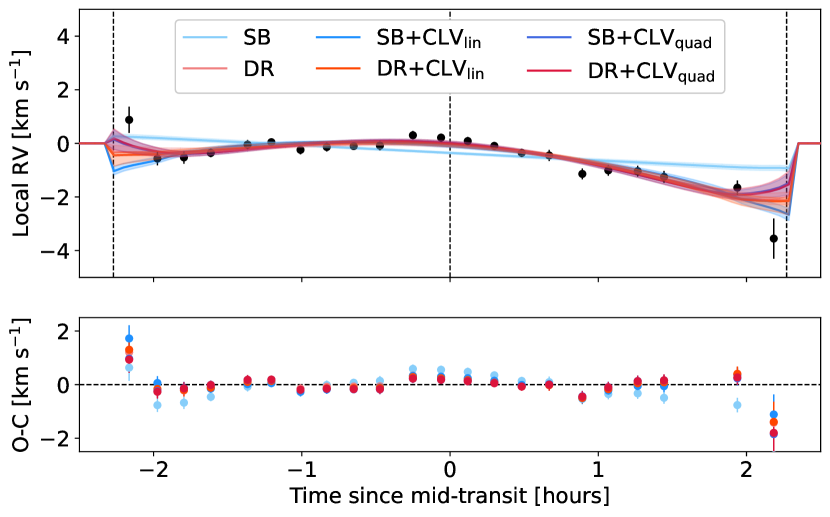
We first found the MAP solution for each model using scipy.optimize.minimize (Virtanen et al., 2020). This best-fit solution was used as the initial location (plus a small Gaussian perturbation) for a MCMC exploration of the posterior. We ran emcee (Foreman-Mackey et al., 2013) as implemented in radvel (Fulton et al., 2018) with 8 ensembles of 32 walkers each for a maximum of 10,000 steps, or until the Gelman–Rubin statistic (G–R; Gelman et al., 2003) was across the ensembles (Ford, 2006). In all cases, the G-R condition for convergence was satisfied and the sampler was terminated with a typical total number of posterior samples around 100,000. A second and final MAP fit was then performed using the median parameter values from the MCMC samples. The MAP fit for each model is plotted over the RV time series in Figure 3, and Table 2 lists our derived best-estimates for each parameter.
4.3 Center-to-Limb Variations
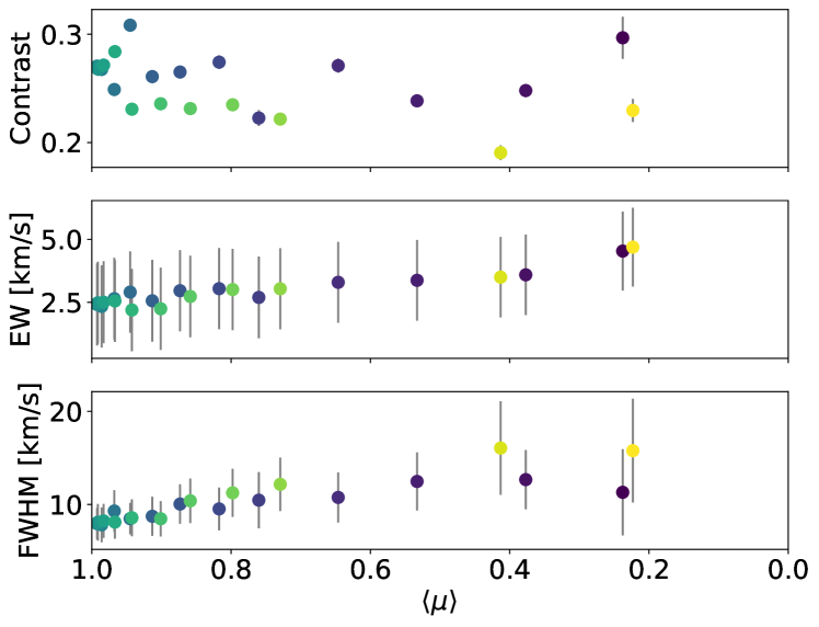
Fig. 4 plots the depth, equivalent width (EW), and full-width-at-half-maximum (FWHM) of the CCF as a function of . A strong trend in the FWHM (Pearson correlation coefficient R=-0.87, p-value of ) and the EW (R=-0.94, p-value ) can be seen from center to limb, with the local line profiles narrowest at disk center and widening towards disk limb. The RV time series (Figure 3) likewise has significant curvature with a maximum (minimum blueshift) at disk center (mid-transit) and minimum (maximum blueshift) at disk limb (ingress/egress). The CCF contrast is only marginally correlated with CLV position during the first half of the transit (R=0.66, p-value 0.04) and is uncorrelated during the second half of the transit (R=0.03, p-value 0.94).
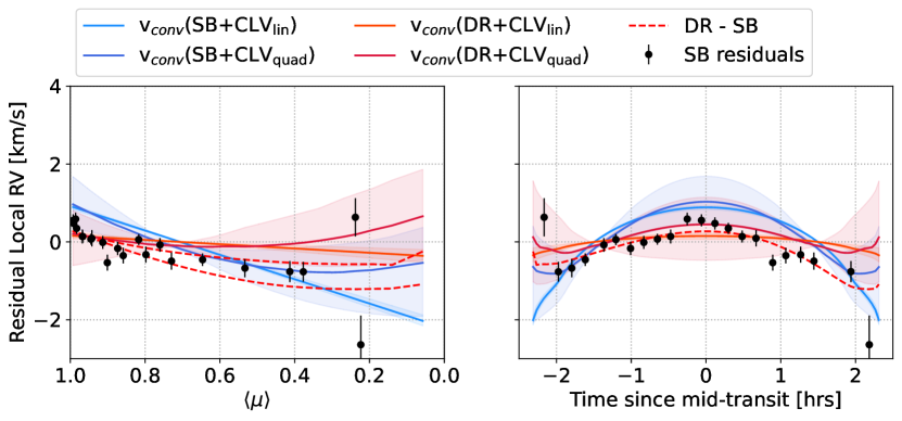
Only CLVs can simultaneously explain the local RV curvature and the change in line width. While differential rotation alone can reproduce the observed curvature in the local RV time series, it cannot explain the large (factor of two) increase in FWHM from disk center to limb. Beeck et al. (2013a) showed using spectral line synthesis in 3D radiative magnetohydrodynamical (MHD) simulations that surface-layer granulation causes the width of spectral lines to increase towards disk limb, an effect that is relatively muted for GKM stars but is significant for F-type stars. The F3 V star in their simulation showed increases to the FWHM of iron lines by a factor of 1.5–2 from disk center to . This effect is caused by the horizontal flows, which dominate the line-of-sight velocity at disk limb, having roughly three times as high a velocity dispersion compared to the vertical velocity (Beeck et al., 2013b). They also found line cores to have a net convective blueshift about 500 m s-1 less (i.e., larger RV) at disk limb than at disk center. We see the opposite in the modelled CLV vs. (Fig. 5) for the SB scenario, whereas in the DR scenario we find negligible convective velocities.
.
| Parameter | Prior | SB | SB+CLV | SB+CLV | DR | DR+CLV | DR+CLV |
|---|---|---|---|---|---|---|---|
| Model Parameters | |||||||
| (∘) | — | ||||||
| (km s-1) | Gaussian(10.4, 1) | ||||||
| Uniform(0, 1) | |||||||
| Uniform(-1, 1) | |||||||
| Uniform(-1, 1) | — | — | — | ||||
| (km s-1) | Uniform(-10, 10) | — | — | ||||
| (km s-1) | Uniform(-10, 10) | — | — | — | — | ||
| BIC | — | 74.0 | 9.2 | 0.0 | 1.5 | 3.4 | 3.0 |
| AIC | — | 73.0 | 8.5 | 0.0 | 0.7 | 3.4 | 4.3 |
| Derived | |||||||
| (∘) | — |
∗Uniform in .
4.4 Model Comparison
We computed the Bayesian information criterion (BIC) and Akaike information criterion (AIC) for each model. Their relative values to the minimum are listed in Table 2. The only model that is confidently ruled out is SB rotation with no CLV, at BIC=74 and AIC=73. The slightly preferred model is SB rotation with CLVs quadratic in . The models with DR all have BIC and AIC , and thus are statistically similar descriptions of the model.
The model with DR alone requires an extremely high values of , in the 0.9–1 range. While it is not impossible for the stellar poles to rotate at just 10% the rate of the equator, it seems extremely unlikely for a star to have a rotational shear of this magnitude. Slowly rotating ( km s-1) F-type stars do commonly show signs of differential rotation (), whereas rapid rotators do not (Reiners & Schmitt, 2003). Our analysis of the TESS photometry in Section 2.1 more likely places KELT-18 in the former category of slow rotators. Interestingly, the DR model with linear CLVs finds a smaller , and the flexibility of the quadratic CLV model results in an unconstrained , as the two effects are degenerate. In contrast, the SB models rely on strong CLVs to generate the measured curvature (Fig. 5). It is therefore ambiguous from the RV time series alone whether the curvature is coming from a significant differential rotation, CLVs, or a mixture of the two. The difference between these two cases is greatest at low , i.e. near the disk limb. This is where CLV effects are strongest whereas DR is only affected by the subplanet stellar latitude. However, the data near disk limb (i.e. near ingress/egress) are the lowest S/N observations, weakening their utility as a discriminatory lever-arm.
If the star is differentially rotating, the varying line-of-sight rotational velocities as a function of stellar latitude break the degeneracy, allowing an independent constraint on the stellar inclination. In the DR-only model, the resulting stellar inclination is . This value is in agreement with the 5–30∘ range expected from the estimated rotation period and known (Section 2.1). Consequently, the true 3D obliquity can be determined via the equation
| (5) |
The corresponding values of for each of fitted models are listed in Table 2. For the SB models, the posterior in is unconstrained (uniform in 0 to 1) so this represents the maximally uncertain value of . For instance, if we adopt from the best-fitting SB+CLV model, and take to be isotropic (uniform in ), then . If instead we take to be isotropic within 5–30∘ as suggested from photometric analyses, we get . Our estimated obliquity measurements are consistent within across all models, thus we adopt the SB+CLV model as our preferred fit as it is both the best-fitting model by the BIC and AIC tests, is more physically justified than the models, and utilizes photometric constraints on the stellar inclination rather than the values from the RRM posteriors.
5 Orbital Dynamics
KELT-18 b joins the population of close-in planets orbiting hot stars in polar orbits (Albrecht et al., 2022a). There are no other known transiting planets in the system (Maciejewski, 2020), though there is a stellar companion, KELT-18 B (Section 2.2). It is likely that KELT-18 B influenced the orbital evolution of KELT-18 b. In this section we examine possible mechanisms.
Hierarchical triple systems such as KELT-18, KELT-18 b, and KELT-18 B will experience von-Zeipel-Kozai-Lidov (ZKL) oscillations if the mutual inclination between the two orbiting bodies is larger than (Naoz, 2016). ZKL oscillations are usually suppressed for planets on HJ-like orbits because of the general relativistic precession of the argument of periapsis. However ZKL oscillations may have taken place early in the system’s history if KELT-18 b formed at a further orbital distance. Fabrycky & Tremaine (2007) showed that such a scenario can lead to HEM, producing the HJ we see today in a close-in, highly misaligned orbit.
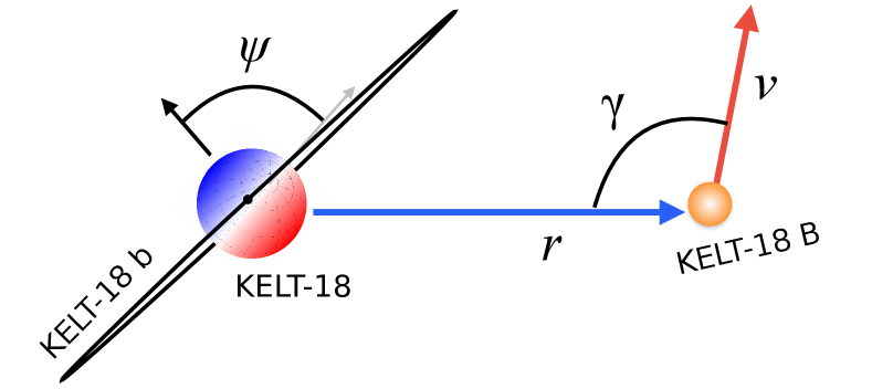
The Gaia astrometry enables a constraint on the inclination of KELT-18 B’s orbit. The angle between the vector connecting the astrometric positions of the two stars () and the difference in velocity vectors (), called (e.g., Tokovinin & Kiyaeva, 2015; Hwang et al., 2022, see Fig. 7), encodes information about the companion’s orbital inclination (though is degenerate with eccentricity). If or , then the companion’s orbit is viewed edge-on. Otherwise, the companion’s orbit may be viewed face-on or at some intermediate inclination. Since KELT-18 b transits, we know it has , so can test for mutual (mis)alignment. We calculated , which is most consistent with a low orbital inclination for a circular KELT-18 B and thus a large mutual inclination (Fig. 7).
For ZKL to excite KELT-18 b’s orbit, it must have formed far away from its host star. By equating the timescales for GR precession and ZKL oscillations, one can solve for the minimum orbital separation at which ZKL oscillations are not quenched by GR (Eq. 4 of Dong et al., 2014). We computed this value for the KELT-18 system and obtained AU. In other words, if KELT-18 b was born beyond AU, for instance via traditional core accretion beyond the ice-line, then it could have plausibly migrated to its current orbit via ZKL-induced HEM. B22 calculated typical minimum formation distances of 0.5–10 AU across the broader population of HJs for binary star induced ZKL HEM migration, which conspicuously aligns with the peak in cold Jupiter occurrence around 1–10 AU (Fulton et al., 2021). Future studies of KELT-18 b’s atmosphere via transmission spectroscopy (Householder, A., Dai, F., et al. in prep) will seek additional evidence for KELT-18 b’s birth conditions by measuring its inventory of refractory and volatile elements, the fingerprints of the original planetary building blocks (Lothringer et al., 2021).
It may also be the case that KELT-18 b formed in a protoplanetary that was primordially misaligned, as can be the case when an outer stellar companion is involved (Batygin, 2012). Alternatively, the stellar companion may have torqued the outer regions of the protoplanetary disk into a misalignment, producing a broken protoplanetary disk which itself can play the role of an outer perturber in exciting large stellar obliquities (Epstein-Martin et al., 2022). Vick et al. (2023) showed that such an initial configuration, in which the star has a disk-induced nonzero obliquity relative to the proto-HJ before ZKL oscillations induced by the stellar companion initiate HEM, the final obliquity distribution of the HJ is broadly retrograde with a peak near polar orbits. This is in contrast with the classical picture of ZKL starting with initially aligned planetary orbits, which produce HJs with a bimodal obliquity distribution near 40∘ and 140∘ (Anderson et al., 2016). Thus it may be that the orbit of KELT-18 b was already misaligned with the star’s rotation before undergoing HEM into its present day HJ orbit, the result of which is an orbit with rather than 40∘ or 140∘.
6 Conclusion
We have presented the first science results from KPF on the Keck-I telescope: a transit of the inflated ultra-hot Jupiter KELT-18 b. We found the orbit to be nearly perpendicular to the stellar equatorial plane: . This result is robust to model choice and is largely constrained by the tight posterior on and the relatively low value of . Taken in context with the binary stellar companion, which we find to be on a likely bound orbit that could be orthogonal to KELT-18 b’s orbit, a history of ZKL-induced HEM is plausible if KELT-18 b formed beyond about 6 AU from its host star. Our main observational takeaways are as follows:
-
•
We searched the available TESS photometry for clues as to the rotation period of the host star and found evidence for modulation around 5 days. We did not see variability at 0.707 days as previously reported by M17 using KELT photometry. Both values are consistent with the tendency for F-type stars to have day rotation periods, and when combined with the measured imply a near pole-on viewing geometry ().
-
•
The stellar neighbor KELT-18 B is highly likely to be a bound companion, based on Gaia DR3 astrometry. Its orbit is also likely orthogonal to KELT-18 b’s orbit, based on the angle between the on-sky position vector and proper motion vectors.
-
•
We observed evidence of CLVs, as traced by the FWHM of the local line profile beneath the planet’s shadow. The FWHM increased towards the disk limb by nearly a factor of two, in agreement with previous 3D MHD simulations of velocity flows in the near-surface layers of F-type stellar atmospheres.
-
•
We modelled the centroid of the local line profile using the RRM technique and found that either strong differential rotation () or CLVs are needed to explain the curvature in the local RV time series. However, all of the models produce consistent, well-constrained posteriors for the sky-projected obliquity. Ambiguity between DR and CLVs is a common challenge of the RRM technique (see e.g. Roguet-Kern et al., 2022; Doyle et al., 2023) and is complicated by the uncertainty in the stellar inclination (and thus the stellar latitudes occulted). A firm detection of a stellar rotation period from additional photometry would enable a better constraint of the degree of DR needed to explain the data. As it stands, the polar transiting geometry requires a low (near pole-on) stellar inclination in order to generate the observed curvature in the local RV timeseries, with maximum blueshift occulted at ingress/egress and near-zero velocity occulted at mid-transit. An edge on stellar inclination would produce the opposite effect, since the lowest velocity latitudes at the poles would instead be occulted at ingress/egress, while the maximum velocity latitude (the equator) would be occulted at mid-transit. If KELT-18 does have an edge-on stellar inclination, then DR would be inconsistent with the data and CLVs would be strongly favored.
-
•
The 3D orbital geometry of the KELT-18 system is explainable by a history of ZKL-induced migration, providing support for the HEM formation pathway for HJs. Future work will further test this by inventorying the elemental abundances in KELT-18’s atmosphere, connecting the planet to the disk in which it formed.
7 Acknowledgements
We are grateful to Heather Cegla and Michael Palumbo for illuminating discussions on center-to-limb variations. Some of the data presented herein were obtained at Keck Observatory, which is a private 501(c)3 non-profit organization operated as a scientific partnership among the California Institute of Technology, the University of California, and the National Aeronautics and Space Administration. The Observatory was made possible by the generous financial support of the W. M. Keck Foundation. Keck Observatory occupies the summit of Maunakea, a place of significant ecological, cultural, and spiritual importance within the indigenous Hawaiian community. We understand and embrace our accountability to Maunakea and the indigenous Hawaiian community, and commit to our role in long-term mutual stewardship. We are most fortunate to have the opportunity to conduct observations from Maunakea.
R.A.R. acknowledges support from the National Science Foundation through the Graduate Research Fellowship Program (DGE 1745301). A.W.H. acknowledges funding support from NASA award 80NSSC24K0161 and the JPL President’s and Director’s Research and Develop Fund. This paper made use of data collected by the TESS mission and are publicly available from the Mikulski Archive for Space Telescopes (MAST) operated by the Space Telescope Science Institute (STScI). All the TESS data used in this paper can be found in MAST: http://dx.doi.org/t9-nmc8-f686 (catalog 10.17909/t9-nmc8-f686) (MAST, 2021). This research was carried out, in part, at the Jet Propulsion Laboratory and the California Institute of Technology under a contract with the National Aeronautics and Space Administration and funded through the President’s and Director’s Research & Development Fund Program.
References
- Albrecht et al. (2012) Albrecht, S., Winn, J. N., Johnson, J. A., et al. 2012, ApJ, 757, 18
- Albrecht et al. (2022a) Albrecht, S. H., Dawson, R. I., & Winn, J. N. 2022a, PASP, 134, 082001
- Albrecht et al. (2022b) Albrecht, S. H., Marcussen, M. L., Winn, J., Dawson, R., & Knudstrup, E. 2022b, in Bulletin of the American Astronomical Society, Vol. 54, 501.05
- Anderson et al. (2016) Anderson, K. R., Storch, N. I., & Lai, D. 2016, MNRAS, 456, 3671
- Astropy Collaboration et al. (2013) Astropy Collaboration, Robitaille, T. P., Tollerud, E. J., et al. 2013, A&A, 558, A33
- Astropy Collaboration et al. (2018) Astropy Collaboration, Price-Whelan, A. M., Sipőcz, B. M., et al. 2018, AJ, 156, 123
- Astropy Collaboration et al. (2022) Astropy Collaboration, Price-Whelan, A. M., Lim, P. L., et al. 2022, ApJ, 935, 167
- Baranne et al. (1996) Baranne, A., Queloz, D., Mayor, M., et al. 1996, A&AS, 119, 373
- Batygin (2012) Batygin, K. 2012, Nature, 491, 418
- Beeck et al. (2013a) Beeck, B., Cameron, R. H., Reiners, A., & Schüssler, M. 2013a, A&A, 558, A49. https://doi.org/10.1051/0004-6361/201321345
- Beeck et al. (2013b) Beeck, B., Cameron, R. H., Reiners, A., & Schüssler, M. 2013b, A&A, 558, A48. https://doi.org/10.1051/0004-6361/201321343
- Behmard et al. (2022) Behmard, A., Dai, F., & Howard, A. W. 2022, The Astronomical Journal, 163, 160. https://dx.doi.org/10.3847/1538-3881/ac53a7
- Blunt et al. (2023) Blunt, S., Carvalho, A., David, T. J., et al. 2023, The Astronomical Journal, 166, 62. https://dx.doi.org/10.3847/1538-3881/acde78
- Bouchy et al. (2001) Bouchy, F., Pepe, F., & Queloz, D. 2001, Å, 374, 733. https://doi.org/10.1051/0004-6361:20010730
- Bouma et al. (2023) Bouma, L. G., Palumbo, E. K., & Hillenbrand, L. A. 2023, ApJ, 947, L3
- Brown et al. (1991) Brown, T. M., Gilliland, R. L., Noyes, R. W., & Ramsey, L. W. 1991, ApJ, 368, 599
- Caldwell et al. (2020) Caldwell, D. A., Tenenbaum, P., Twicken, J. D., et al. 2020, Research Notes of the American Astronomical Society, 4, 201
- Cegla et al. (2016) Cegla, H. M., Lovis, C., Bourrier, V., et al. 2016, A&A, 588, A127
- Dawson (2014) Dawson, R. 2014, Astrophysical Journal Letters, 790, doi:10.1088/2041-8205/790/2/L31
- Dawson & Johnson (2018) Dawson, R. I., & Johnson, J. A. 2018, ARA&A, 56, 175
- Dong & Foreman-Mackey (2023) Dong, J., & Foreman-Mackey, D. 2023, AJ, 166, 112
- Dong et al. (2014) Dong, S., Katz, B., & Socrates, A. 2014, ApJ, 781, L5
- Doyle et al. (2023) Doyle, L., Cegla, H. M., Anderson, D. R., et al. 2023, Monthly Notices of the Royal Astronomical Society, 522, 4499. https://doi.org/10.1093/mnras/stad1240
- Epstein-Martin et al. (2022) Epstein-Martin, M., Becker, J., & Batygin, K. 2022, The Astrophysical Journal, 931, 42. https://dx.doi.org/10.3847/1538-4357/ac5b79
- Fabrycky & Tremaine (2007) Fabrycky, D., & Tremaine, S. 2007, ApJ, 669, 1298
- Ford (2006) Ford, E. B. 2006, ApJ, 642, 505
- Foreman-Mackey (2016) Foreman-Mackey, D. 2016, JOSS, 1
- Foreman-Mackey et al. (2013) Foreman-Mackey, D., Hogg, D. W., Lang, D., & Goodman, J. 2013, PASP, 125, 306
- Fulton et al. (2018) Fulton, B. J., Petigura, E. A., Blunt, S., & Sinukoff, E. 2018, PASP, 130, 044504
- Fulton et al. (2021) Fulton, B. J., Rosenthal, L. J., Hirsch, L. A., et al. 2021, The Astrophysical Journal Supplement Series, 255, 14. https://dx.doi.org/10.3847/1538-4365/abfcc1
- Gaia Collaboration et al. (2023) Gaia Collaboration, Vallenari, A., Brown, A. G. A., et al. 2023, A&A, 674, A1
- Gelman et al. (2003) Gelman, A., Carlin, J. B., Stern, H. S., & Rubin, D. B. 2003, Bayesian Data Analysis, 2nd edn. (Chapman and Hall)
- Gibson et al. (2016) Gibson, S. R., Howard, A. W., Marcy, G. W., et al. 2016, in Society of Photo-Optical Instrumentation Engineers (SPIE) Conference Series, Vol. 9908, Ground-based and Airborne Instrumentation for Astronomy VI, ed. C. J. Evans, L. Simard, & H. Takami, 990870
- Gibson et al. (2018) Gibson, S. R., Howard, A. W., Roy, A., et al. 2018, in Society of Photo-Optical Instrumentation Engineers (SPIE) Conference Series, Vol. 10702, Ground-based and Airborne Instrumentation for Astronomy VII, ed. C. J. Evans, L. Simard, & H. Takami, 107025X
- Gibson et al. (2020) Gibson, S. R., Howard, A. W., Rider, K., et al. 2020, in Society of Photo-Optical Instrumentation Engineers (SPIE) Conference Series, Vol. 11447, Society of Photo-Optical Instrumentation Engineers (SPIE) Conference Series, 1144742
- Harris et al. (2020) Harris, C. R., Millman, K. J., van der Walt, S. J., et al. 2020, Nature, 585, 357–362
- Huber et al. (2017) Huber, D., Zinn, J., Bojsen-Hansen, M., et al. 2017, ApJ, 844, 102
- Hunter (2007) Hunter, J. D. 2007, CSE, 9, 90
- Hwang et al. (2022) Hwang, H.-C., Ting, Y.-S., & Zakamska, N. L. 2022, MNRAS, 512, 3383
- Ito & Ohtsuka (2019) Ito, T., & Ohtsuka, K. 2019, Monographs on Environment, Earth and Planets, 7, 1
- Ivshina & Winn (2022) Ivshina, E. S., & Winn, J. N. 2022, ApJS, 259, 62
- Kjeldsen & Bedding (1995) Kjeldsen, H., & Bedding, T. R. 1995, A&A, 293, 87
- Kolbl et al. (2015) Kolbl, R., Marcy, G. W., Isaacson, H., & Howard, A. W. 2015, AJ, 149, 18
- Kozai (1962) Kozai, Y. 1962, AJ, 67, 591
- Kraft (1967) Kraft, R. P. 1967, ApJ, 150, 551
- Lidov (1962) Lidov, M. 1962, Planet. Space Sci., 9, 719
- Lightkurve Collaboration et al. (2018) Lightkurve Collaboration, Cardoso, J. V. d. M., Hedges, C., et al. 2018, Lightkurve: Kepler and TESS time series analysis in Python, Astrophysics Source Code Library, Astrophysics Source Code Library, ascl:1812.013
- Lothringer et al. (2021) Lothringer, J. D., et al. 2021, ApJ, 914, 12. https://doi.org/10.3847/1538-4357/abf8a9
- Maciejewski (2020) Maciejewski, G. 2020, Acta Astron., 70, 181
- MAST (2021) MAST. 2021, TESS Light Curves - All Sectors, STScI/MAST, doi:10.17909/T9-NMC8-F686. http://archive.stsci.edu/doi/resolve/resolve.html?doi=10.17909/t9-nmc8-f686
- Masuda & Winn (2020) Masuda, K., & Winn, J. N. 2020, AJ, 159, 81
- McLaughlin (1924) McLaughlin, D. B. 1924, ApJ, 60, 22
- McLeod et al. (2017) McLeod, K. K., Rodriguez, J. E., Oelkers, R. J., et al. 2017, AJ, 153, 263
- Naoz (2016) Naoz, S. 2016, ARA&A, 54, 441
- Naoz et al. (2011) Naoz, S., Farr, W. M., Lithwick, Y., Rasio, F. A., & Teyssandier, J. 2011, Nature, 473, 187
- Oh et al. (2017) Oh, S., Price-Whelan, A. M., Hogg, D. W., Morton, T. D., & Spergel, D. N. 2017, The Astronomical Journal, 153, 257. https://dx.doi.org/10.3847/1538-3881/aa6ffd
- pandas development team (2020) pandas development team, T. 2020, pandas-dev/pandas: Pandas, vlatest, Zenodo, doi:10.5281/zenodo.3509134. https://doi.org/10.5281/zenodo.3509134
- Pepe et al. (2002) Pepe, F., Mayor, M., Galland, F., et al. 2002, A&A, 388, 632
- Petigura (2015) Petigura, E. A. 2015, PhD thesis, University of California, Berkeley
- Petrovich et al. (2020) Petrovich, C., Muñoz, D. J., Kratter, K. M., & Malhotra, R. 2020, ApJL, 902, L5
- Pollack et al. (1996) Pollack, J. B., Hubickyj, O., Bodenheimer, P., et al. 1996, Icarus, 124, 62
- Rasio & Ford (1996) Rasio, F. A., & Ford, E. B. 1996, Science, 274, 954
- Reiners & Schmitt (2003) Reiners, A., & Schmitt, J. H. M. M. 2003, A&A, 412, 813. https://doi.org/10.1051/0004-6361:20034255
- Rice et al. (2022) Rice, M., Wang, S., & Laughlin, G. 2022, ApJ, 926, L17
- Ricker et al. (2015) Ricker, G. R., Winn, J. N., Vanderspek, R., et al. 2015, Journal of Astronomical Telescopes, Instruments, and Systems, 1, 014003
- Roguet-Kern et al. (2022) Roguet-Kern, N., Cegla, H. M., & Bourrier, V. 2022, A&A, 661, A97
- Rossiter (1924) Rossiter, R. A. 1924, ApJ, 60, 15
- Rubenzahl (2024) Rubenzahl, R. A. 2024, PhD thesis, California Institute of Technology, doi:10.7907/sgbv-5841
- Rubenzahl et al. (2023) Rubenzahl, R. A., Halverson, S., Walawender, J., et al. 2023, PASP, 135, 125002
- Schlaufman (2010) Schlaufman, K. C. 2010, ApJ, 719, 602
- Siegel et al. (2023) Siegel, J. C., Winn, J. N., & Albrecht, S. H. 2023, ApJ, 950, L2
- Szentgyorgyi & Furész (2007) Szentgyorgyi, A. H., & Furész, G. 2007, in Revista Mexicana de Astronomia y Astrofisica Conference Series, Vol. 28, Revista Mexicana de Astronomia y Astrofisica Conference Series, ed. S. Kurtz, 129–133
- Teyssandier et al. (2013) Teyssandier, J., Naoz, S., Lizarraga, I., & Rasio, F. A. 2013, ApJ, 779, 166
- Tokovinin & Kiyaeva (2015) Tokovinin, A., & Kiyaeva, O. 2015, Monthly Notices of the Royal Astronomical Society, 456, 2070. https://doi.org/10.1093/mnras/stv2825
- Vick et al. (2023) Vick, M., Su, Y., & Lai, D. 2023, ApJ, 943, L13
- Virtanen et al. (2020) Virtanen, P., Gommers, R., Oliphant, T. E., et al. 2020, NatMe, 17, 261
- Vogt et al. (1994) Vogt, S. S., Allen, S. L., Bigelow, B. C., et al. 1994, in Proc. SPIE, Vol. 2198, Instrumentation in Astronomy VIII, ed. D. L. Crawford & E. R. Craine, 362
- von Zeipel (1910) von Zeipel, H. 1910, Astronomische Nachrichten, 183, 345
- Winn et al. (2010) Winn, J. N., Fabrycky, D., Albrecht, S., & Johnson, J. A. 2010, ApJL, 718, L145
- Yee et al. (2017) Yee, S. W., Petigura, E. A., & von Braun, K. 2017, ApJ, 836, 77
Appendix A Sector-by-sector rotation period
Here we present, in Figure 8, the sector-by-sector periodogram of the TESS photometry.