Quantum Simulation via Stochastic Combination of Unitaries
Abstract
Quantum simulation algorithms often require numerous ancilla qubits and deep circuits, prohibitive for near-term hardware. We introduce a framework for simulating quantum channels using ensembles of low-depth circuits in place of many-qubit dilations. This naturally enables simulations of open systems, which we demonstrate by preparing damped many-qubit GHZ states on ibm_hanoi. The technique further inspires two Hamiltonian simulation algorithms with asymptotic independence of the spectral precision, reducing resource requirements by several orders of magnitude for a benchmark system.
Introduction: Linear combination of unitaries (LCU) has proven to be an essential primitive in the design of quantum algorithms Childs and Wiebe (2012); Childs et al. (2017); Low and Chuang (2019); Chakraborty et al. (2019); Wan et al. (2021); Wang et al. (2021); Nguyen et al. (2022); An et al. (2023), enabling the simulation of general operators within a larger, dilated Hilbert space Stinespring (1955); Paulsen (2003); Hu et al. (2020); Langer (1972). While powerful as a theoretical tool, this ancilla-based dilation is often expensive in practice, generating extensive sequences of unitary operators controlled on many qubits. Combined with its need for post-selective measurements Childs and Wiebe (2012), in total LCU can require many repetitions of deep quantum circuits, often infeasible for near-term quantum computers.
In this Letter, we propose a simple stochastic framework for mapping general quantum channels onto single- or no-ancilla circuits, avoiding the expensive many-qubit dilations and post-selection costs of LCU. The stochastic combination of unitaries (SCU) method decomposes a channel into a convex combination of simple transformations, which can then be efficiently sampled and run as independent circuits. This results in low-depth circuits at the cost of additional measurement overhead, invaluable for NISQ-era simulations. Because this technique naturally applies to the simulation of open quantum systems Breuer and Petruccione (2007); Head-Marsden et al. (2021); Schlimgen et al. (2021); Kamakari et al. (2022), we demonstrate its practical advantages by simulating a noisy, eight-qubit entanglement generation process with high accuracy on ibm_hanoi.
Building on this framework, we then propose two stochastic algorithms for Hamiltonian simulation. As one of the most promising applications of quantum technology, Hamiltonian simulation is crucial not only for quantum dynamics Wiebe et al. (2011); Miessen et al. (2023); Ollitrault et al. (2021) but also as a subroutine in ground state estimation Aspuru-Guzik et al. (2005); Dong et al. (2022); Wang et al. (2023); Nam et al. (2020), material characterization Bauer et al. (2020); Lordi and Nichol (2021); De Leon et al. (2021), and combinatorial optimization Farhi et al. (2014); Albash and Lidar (2018). Despite substantial research into Suzuki-Trotter product formulas Lloyd (1996); Suzuki (1991); Childs et al. (2021); Childs and Su (2019), post-Trotter methods Low and Chuang (2017, 2019), and randomized algorithms Campbell (2019); Faehrmann et al. (2022), Hamiltonian simulation remains out of reach for near-term quantum computers. To alleviate these issues, we introduce two simple strategies; one samples a novel, Pauli-based decomposition of the Taylor series, and the other stochastically supplements the Suzuki-Trotter product formulas with higher-order corrections. Remarkably, both algorithms’ circuit depths are asymptotically independent of the target precision, an algorithmic first that enables ultra-precise simulations. We provide resource estimates for simulating the transverse field Ising model, reducing gate counts by up to several orders of magnitude compared to existing methods.
Theory: Quantum channels are completely positive, trace-preserving maps and can be represented using an operator-sum representation
| (1) |
where the Kraus operators satisfy Nielsen and Chuang (2010); Audretsch (2007). We first decompose the Kraus operators into a unitary basis with coefficients . By appropriately normalizing the coefficients, we can then express the channel as a convex combination times a normalization factor :
| (2) |
where . The channel consists of random-unitary terms () and coherence-preserving cross terms ().
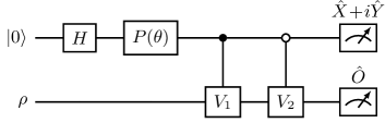
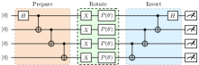
To simulate the channel, we can sample the terms and with their respective probabilities. The random-unitary terms map directly onto circuits consisting of acting on the input state Peetz et al. (2024), and the cross terms map onto circuits of the form shown in Figure 1. In Eq. (2), each cross term and its Hermitian conjugate can be accessed simultaneously via a single measurement of the ancilla qubit Faehrmann et al. (2022).
This stochastic combination of unitaries (SCU) thus generates an ensemble of circuits, with considerably simpler structure and depth compared to linear combination of unitaries (LCU) Childs and Wiebe (2012). Repeatedly sampling this ensemble for samples yields an unbiased estimator of the quantum channel Peetz et al. (2024); Arrasmith et al. (2020), with variance scaling as . In the special case of random-unitary channels, Eq. 2 has unit norm () and excellent scalability Peetz et al. (2024). For general channels, we can mitigate the increased variance via additional measurements, scaling up the number of samples by . For depth-limited devices, this trade-off between low-depth circuits and additional measurement overhead can enable otherwise infeasible simulations.
Damped GHZ Simulation: SCU naturally applies to the simulation of open quantum systems, which we demonstrate by simulating an eight-qubit GHZ state subject to CNOT-induced amplitude damping on ibm_hanoi. The GHZ state is a common example of multipartite entanglement, often analyzed in the context of quantum networks Avis et al. (2023); Meignant et al. (2019); Patil et al. (2022). Realistic networks are subject to noise, such as photon loss and decoherence Covey et al. (2023), and our simulation serves as a guide that could be readily adapted to hardware.
By applying a Hadamard gate and a chain of CNOTs, one prepares the -qubit GHZ state,
| (3) |
Because two-qubit gates are often error-prone in practice, we model a noisy GHZ state with a CNOT-induced amplitude damping channel, with Kraus operators and . That is, after each CNOT in the preparation of , we sample the convex decomposition of the quantum channel as in Eq. (2); we then apply the sampled operators to the target qubit according to SCU. In the Pauli basis, the norms of and are and respectively, making the normalization constant of the channel . For the full -qubit GHZ preparation channel, assuming each CNOT has equal damping strength, the overall normalization constant is thus .
We then measure the fidelity of the prepared noisy state relative to an ideal state via a modified version of multiple quantum coherences (MQC) Gärttner et al. (2018), detailed in the Supplemental Materials. Following the approaches of Wei et al. (2020); Mooney et al. (2021), we expand the fidelity as
| (4) |
In this sum, the all-zero and all-one populations are directly observable in the standard basis. The third and fourth terms are coherences, accessible via MQC. Specifically, the MQC circuit shown in (Wei et al., 2020, Figure 2) gives the signal , and we obtain the coherences via Fourier transform of this signal (Wei et al., 2020, Eq. (2)). As discussed in the Supplementary Materials, the inversion stage of our MQC circuit exactly mirrors the preparation phase, including any sampled damping operators. We note that this technique generalizes the use of MQC to arbitrary channels, expanding beyond its current scope Gärttner et al. (2018).
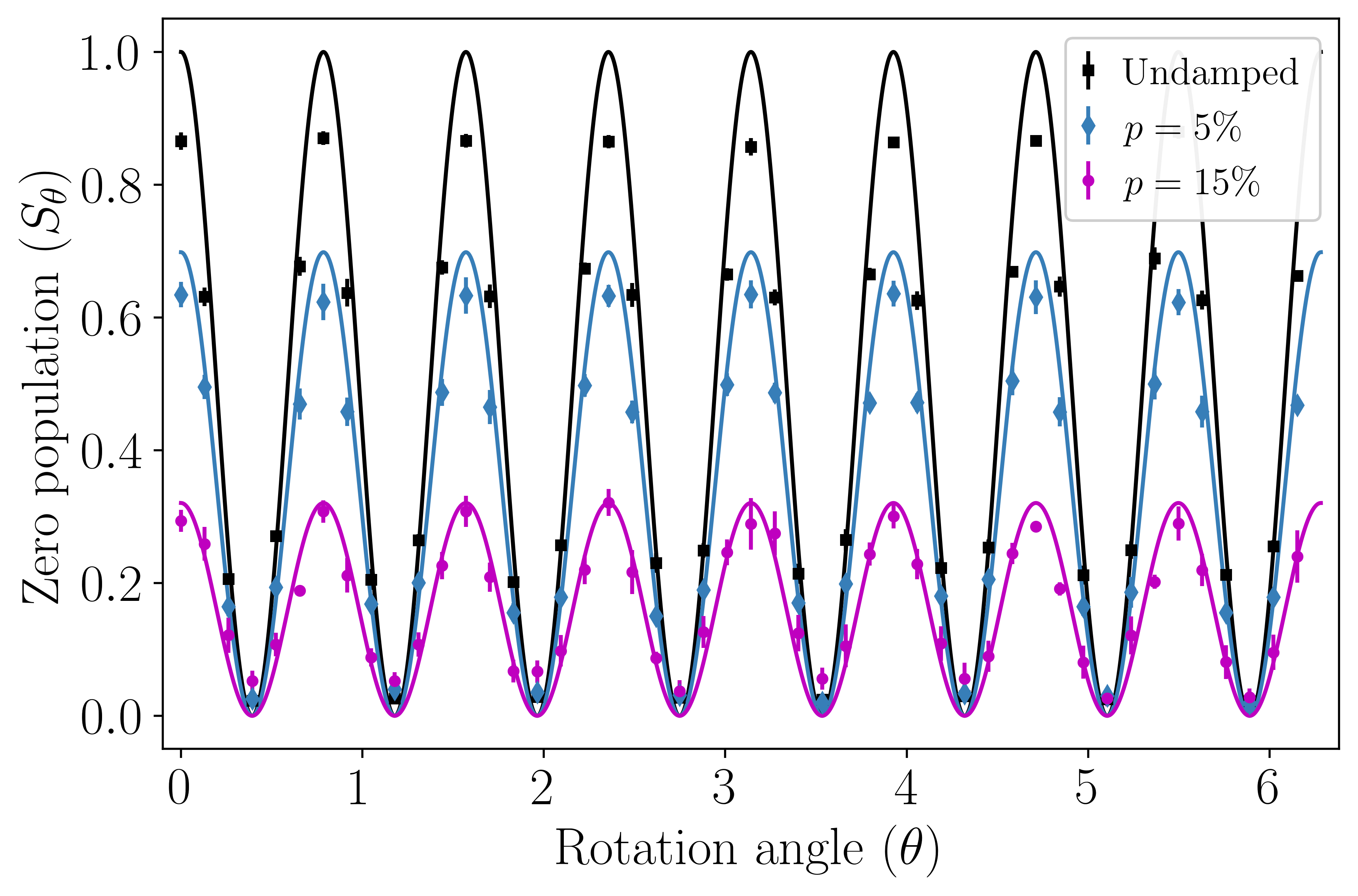
For a damped GHZ state, the analytically predicted signal is the ideal GHZ sinusoid together with a damping prefactor,
| (5) |
In Figure 2, we plot the MQC signal for different damping strengths , comparing experimental results from ibm_hanoi with analytically predicted signals. This simulation gives excellent theoretical agreement in spite of the additional variance induced by SCU.
Finally, we Fourier transform these signals to compute the fidelity . For damping strengths , we respectively measure the fidelities over five runs. These closely match the ideal predictions of , up to a slight offset due to device noise.
Compared to a direct LCU approach, SCU results in much simpler circuits, with reasonable sampling overhead for small damping strengths. Notably, amplitude damping also has tailor-made circuits which outperform direct LCU. For example, the approach in Rost et al. (2020) compiles to four CNOT gates for each instance of damping, compared to CNOT gates on average with SCU. Concretely, in the eight-qubit GHZ simulation, the base MQC circuit with no damping requires 14 CNOTs. To include damping at , the implementation in Rost et al. (2020) would require additional CNOTs compared to only on average with SCU, a massive improvement that enables an otherwise prohibitive simulation. We provide further resource analysis in the Supplemental Materials.
Hamiltonian Simulation: Building on this stochastic framework, we introduce two algorithms for Hamiltonian simulation: 1) convex Taylor sampling (CTS) and 2) stochastically enhanced product formulas. In each algorithm, we expand time evolution as a probabilistic combination of quantum operations,
| (6) |
From this form, we approximate the channel via randomized sampling of and , obtaining left/right gate pairs for each time step. These transformations are then simulated via SCU with measurement overhead . While many such decompositions exist, we investigate expansions with minimal spectral error and normalization constant . Both of the algorithms have gate complexities which are asymptotically independent of the target precision, thus enabling simulations with low spectral error requirements.
Convex Taylor Sampling: The following theorem (proven in the Supplementary Materials) gives a novel decomposition of the Taylor series of a time evolution operator, with inspiration from Ref. Wan et al. (2022). We use this decomposition to construct a simulation algorithm, with step-by-step instructions in Figure 3.
Input: A time-independent Hamiltonian decomposed into Pauli strings, . Output: A sequence of left/right gate pairs. 1. Discretize the time evolution into time steps, 2. Classically compute a convex approximation of to truncation order : 3. Repeatedly sample and to generate left/right pairs of quantum gates.
Theorem 1: For a Hermitian operator and real parameter ,
| (7) |
where , , and represent Pauli strings up to a negative sign. Further, and are bounded as and , where .
Theorem 1 expresses the Taylor series as a convex combination of unitary operators up to an overall norm. This form lends itself to convex Taylor sampling (CTS), an algorithm that leverages SCU to independently sample the left and right propagators, and . Specifically, for a time step , we truncate the expansion in Theorem 1 to order and normalize by the overall norm . We then sample the resulting convex combination
| (8) |
where the coefficients and form a probability distribution. Independently, we sample to obtain an overall transformation of the form , as implemented in Figure 1. To minimize simulation error, we discretize into time steps as follows:
| (9) |
where is the normalization constant for the full channel. We see that for a tolerated error , CTS requires time steps.

To mitigate the additional variance induced by the normalization constant , we budget a maximum measurement overhead, creating a second constraint on the number of time steps. Because the leading order contribution to is quadratic, we get
| (10) |
Thus, to limit the measurement overhead to , we require time steps. For , this overhead constraint is asymptotically dominant over the constraint on the spectral precision.
The CTS algorithm is closely related to qDRIFT, a highly influential stochastic simulation algorithm Campbell (2019). qDRIFT approximates the time propagator to first order in time as a random-unitary channel, requiring time steps Campbell (2019). While both algorithms’ gate complexities scale quadratically in and , CTS is asymptotically independent of the spectral precision and instead scales with the maximum tolerated normalization constant . This difference is crucial because and typically differ by several orders of magnitude.
Stochastically Enhanced Product Formulas: The Suzuki-Trotter product formulas are perhaps the most well-known algorithms for Hamiltonian simulation Lloyd (1996); Suzuki (1991). For the Hamiltonian , the first-order product formula approximates its time evolution to as
| (11) |
More generally, denotes the -th order product formula. Higher-order product formulas correct asymmetries from the operators not commuting.
We can enhance these formulas by stochastically implementing their remainders as higher-order error corrections. For example, the leading error of the first-order product formula is a sum of commutators, ; more generally, we can compute the remainders of a -th order product formula up to a truncation order . This yields a convex combination up to the normalization constant :
| (12) |
where the Pauli strings are computed from the remainder expressions. For a desired precision , this stochastically enhanced product formula requires time steps.
Once again, the overall normalization constant determines our sampling overhead, with asymptotic scaling determined by the leading-order remainder. For the enhanced -th order product formula,
| (13) |
where is the norm of the nested commutator expression in Ref. Childs et al. (2021). Thus, we require time steps to bound the measurement overhead to . This is asymptotically dominant over the constraint on spectral precision.
Transverse Field Ising Simulation: To highlight the performance of these approaches, we compare gate costs for simulating the transverse field Ising model (TFIM). The TFIM Hamiltonian is , where is the exchange interaction parameter and quantifies the strength of the transverse magnetic field.
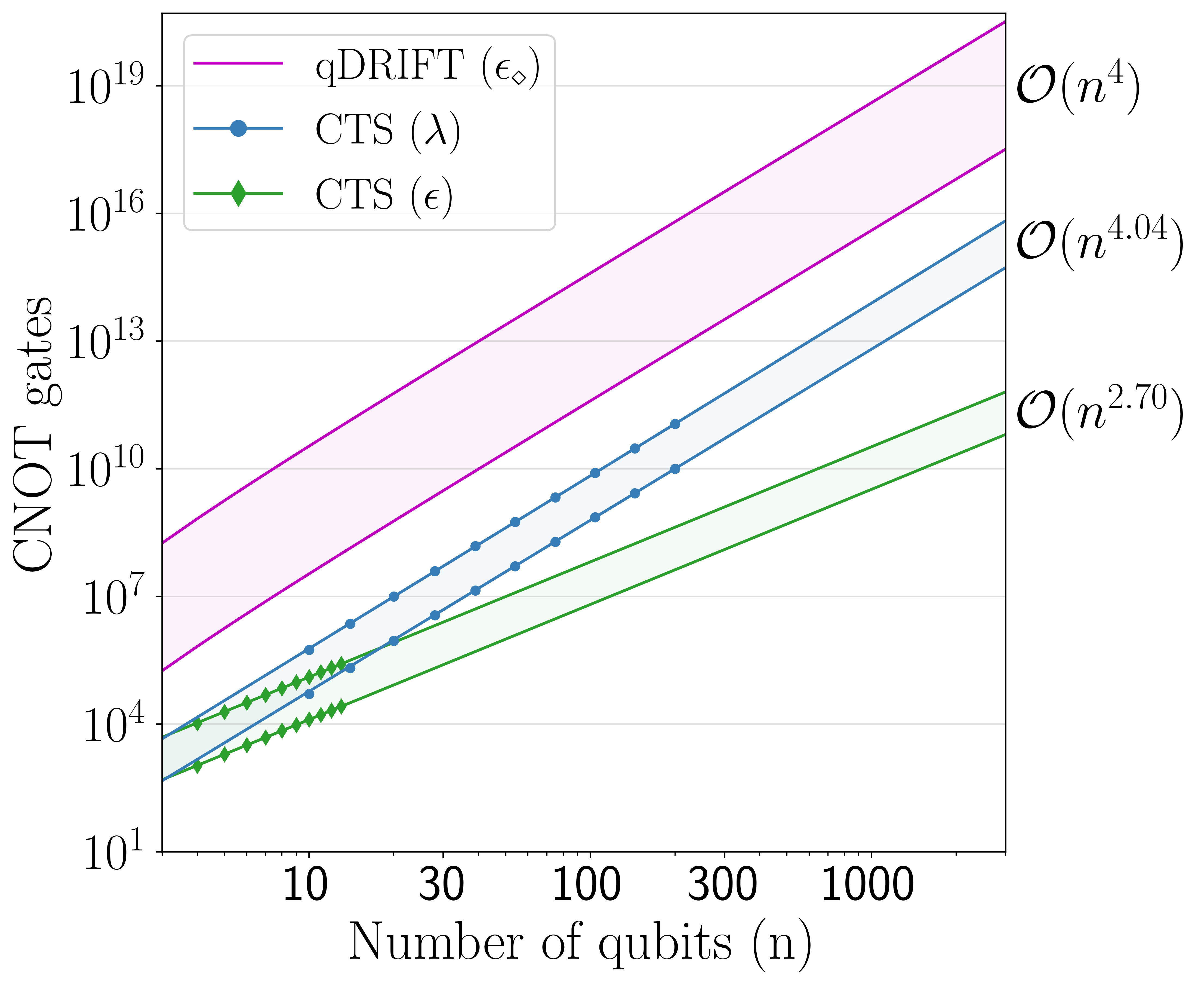
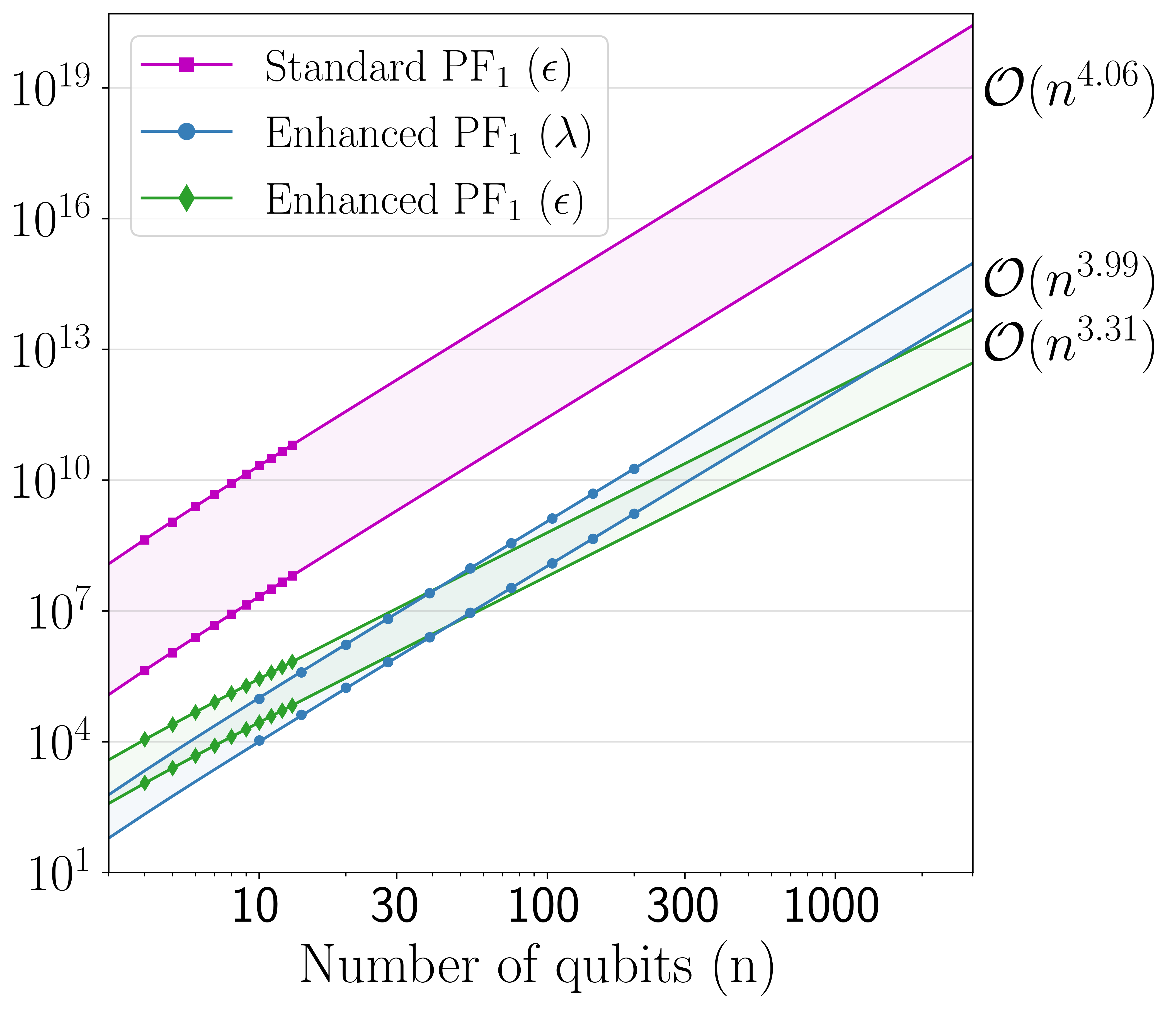
We compute the number of CNOT gates required to simulate the TFIM for system size , evolution time , and model parameters and , following Ref. Childs et al. (2018). To compare dependencies on spectral precision and normalization constant , we consider the parameter ranges and . Our resource estimates for all algorithms are combined in Figure 4. For a broad range of sizes, our algorithms reduce the CNOT counts by several orders of magnitude. This difference is particularly pronounced for simulations with low spectral error, i.e. , due to our algorithms’ asymptotic independence of spectral precision. Importantly, for many parameter choices, the reductions in depth exceed the measurement overhead of , improving the overall runtime.
To bound the sampling overhead, we evaluate each algorithms’ series expansion to truncation order , using Pauli string algebra rather than a matrix representation. For CTS and the stochastically enhanced first-order product formula, we compute the respective expansions to order up to 200 qubits. For the enhanced second-order product formula, we compute corrections to order and use Markov sampling for orders up to 50 qubits, as detailed in the Supplementary Materials.
By properly including cross terms, our proposed algorithms model time evolution coherently, enabling empirical resource estimates with the spectral norm Chen et al. (2021). In contrast, qDRIFT estimates require the diamond norm, which is challenging to compute for more than a few qubits. Following Campbell’s paper Campbell (2019), we instead analytically bound the number of gates as , where is the norm of the Hamiltonian and is the diamond norm error bound. To enable comparisons in Figure 4, we apply a bound on the diamond norm described in Refs. Chen et al. (2021); Kiss et al. (2023). For a target unitary channel and a probabilistic ensemble of unitary channels ,
| (14) |
Discussion and Conclusion: We first demonstrated SCU in the context of open quantum systems, simulating an eight-qubit, noisy GHZ state with high accuracy on ibm_hanoi. SCU significantly reduced circuit depths while maintaining reasonable measurement costs, enabling an otherwise prohibitive simulation. Beyond this example, one could similarly model time-dependent bath interactions via sequential sampling of time-dependent unitary decompositions. More broadly, this framework can be applied to any transformation, opening the door to applications beyond quantum simulation.
In applying SCU to the problem of Hamiltonian simulation, we showed stochastically executing high-order series operators can significantly reduce CNOT costs, with interesting parallels to composite simulation algorithms Hagan and Wiebe (2023). These ideas can similarly apply to higher-order product formulas as well as different systems of interest, such as fermionic and power law Hamiltonians. The algorithms’ asymptotic independence of target precision is particularly attractive for simulations requiring low spectral error.
As seen in the Pauli decompositions and as further discussed in the Supplementary Materials, the measurement overhead of SCU can be substantially impacted by the choice of unitary bases and the resultant norm of the unitary decomposition. Selecting a proper unitary basis or utilizing Hamiltonian decomposition techniques Loaiza et al. (2023) could further lower the norm and thus the measurement overhead.
The SCU approach provides a general framework for realizing quantum channels as ensembles of simple quantum circuits. SCU repeatedly samples a sub-normalized channel’s convex unitary decomposition, yielding unitary gates for the random-unitary terms and single-ancilla dilations for the cross terms. This approach mitigates the need for the large ancilla networks and multi-controlled gates required in techniques like linear combination of unitaries Childs and Wiebe (2012), quantum signal processing Low and Chuang (2017), and qubitization Low and Chuang (2019). Instead, SCU generates low-depth circuits at the cost of additional measurements, a valuable trade-off for near-term quantum devices.
Acknowledgements: This work is supported by an NSF CAREER Award under Grant No. NSF-ECCS-1944085 and the NSF CNS program under Grant No. 2247007. The authors acknowledge the use of IBM Quantum services for this work. The views expressed are those of the authors, and do not reflect the official policy or position of IBM or the IBM Quantum team.
References
- Childs and Wiebe (2012) A. M. Childs and N. Wiebe, Quantum Information & Computation 12, 901 (2012).
- Childs et al. (2017) A. M. Childs, R. Kothari, and R. D. Somma, SIAM Journal on Computing 46, 1920 (2017).
- Low and Chuang (2019) G. H. Low and I. L. Chuang, Quantum 3, 163 (2019).
- Chakraborty et al. (2019) S. Chakraborty, A. Gilyén, and S. Jeffery, in DROPS-IDN/v2/document/10.4230/LIPIcs.ICALP.2019.33 (Schloss Dagstuhl – Leibniz-Zentrum für Informatik, 2019).
- Wan et al. (2021) L.-C. Wan, C.-H. Yu, S.-J. Pan, S.-J. Qin, F. Gao, and Q.-Y. Wen, Physical Review A 104, 062414 (2021).
- Wang et al. (2021) S. Wang, Z. Wang, G. Cui, S. Shi, R. Shang, L. Fan, W. Li, Z. Wei, and Y. Gu, Quantum Information Processing 20, 270 (2021).
- Nguyen et al. (2022) Q. T. Nguyen, B. T. Kiani, and S. Lloyd, Quantum 6, 876 (2022).
- An et al. (2023) D. An, J.-P. Liu, and L. Lin, Physical Review Letters 131, 150603 (2023).
- Stinespring (1955) W. F. Stinespring, in Proceedings of the American Mathematical Society, Vol. 6 (1955) pp. 211–216.
- Paulsen (2003) V. Paulsen, Completely Bounded Maps and Operator Algebras, Cambridge Studies in Advanced Mathematics (Cambridge University Press, Cambridge, 2003).
- Hu et al. (2020) Z. Hu, R. Xia, and S. Kais, Scientific Reports 10, 3301 (2020).
- Langer (1972) H. Langer, ZAMM - Zeitschrift für Angewandte Mathematik und Mechanik 52, 501 (1972).
- Breuer and Petruccione (2007) H.-P. Breuer and F. Petruccione, The Theory of Open Quantum Systems (Oxford University Press, Oxford, New York, 2007).
- Head-Marsden et al. (2021) K. Head-Marsden, J. Flick, C. J. Ciccarino, and P. Narang, Chemical Reviews 121, 3061 (2021).
- Schlimgen et al. (2021) A. W. Schlimgen, K. Head-Marsden, L. M. Sager, P. Narang, and D. A. Mazziotti, Physical Review Letters 127, 270503 (2021).
- Kamakari et al. (2022) H. Kamakari, S.-N. Sun, M. Motta, and A. J. Minnich, PRX Quantum 3, 010320 (2022).
- Wiebe et al. (2011) N. Wiebe, D. W. Berry, P. Hoyer, and B. C. Sanders, Journal of Physics A: Mathematical and Theoretical 44, 445308 (2011), arXiv:1011.3489 [math-ph, physics:quant-ph].
- Miessen et al. (2023) A. Miessen, P. J. Ollitrault, F. Tacchino, and I. Tavernelli, Nature Computational Science 3, 25 (2023).
- Ollitrault et al. (2021) P. J. Ollitrault, A. Miessen, and I. Tavernelli, Accounts of Chemical Research 54, 4229 (2021).
- Aspuru-Guzik et al. (2005) A. Aspuru-Guzik, A. D. Dutoi, P. J. Love, and M. Head-Gordon, Science 309, 1704 (2005).
- Dong et al. (2022) Y. Dong, L. Lin, and Y. Tong, PRX Quantum 3, 040305 (2022).
- Wang et al. (2023) G. Wang, D. S. França, R. Zhang, S. Zhu, and P. D. Johnson, Quantum 7, 1167 (2023).
- Nam et al. (2020) Y. Nam, J.-S. Chen, N. C. Pisenti, K. Wright, C. Delaney, D. Maslov, K. R. Brown, S. Allen, J. M. Amini, J. Apisdorf, K. M. Beck, A. Blinov, V. Chaplin, M. Chmielewski, C. Collins, S. Debnath, K. M. Hudek, A. M. Ducore, M. Keesan, S. M. Kreikemeier, J. Mizrahi, P. Solomon, M. Williams, J. D. Wong-Campos, D. Moehring, C. Monroe, and J. Kim, npj Quantum Information 6, 1 (2020).
- Bauer et al. (2020) B. Bauer, S. Bravyi, M. Motta, and G. K.-L. Chan, Chemical Reviews 120, 12685 (2020).
- Lordi and Nichol (2021) V. Lordi and J. M. Nichol, MRS Bulletin 46, 589 (2021).
- De Leon et al. (2021) N. P. De Leon, K. M. Itoh, D. Kim, K. K. Mehta, T. E. Northup, H. Paik, B. S. Palmer, N. Samarth, S. Sangtawesin, and D. W. Steuerman, Science 372, eabb2823 (2021).
- Farhi et al. (2014) E. Farhi, J. Goldstone, and S. Gutmann, “A Quantum Approximate Optimization Algorithm,” (2014), arXiv:1411.4028 [quant-ph].
- Albash and Lidar (2018) T. Albash and D. A. Lidar, Reviews of Modern Physics 90, 015002 (2018).
- Lloyd (1996) S. Lloyd, Science 273, 1073 (1996).
- Suzuki (1991) M. Suzuki, Journal of Mathematical Physics 32, 400 (1991).
- Childs et al. (2021) A. M. Childs, Y. Su, M. C. Tran, N. Wiebe, and S. Zhu, Physical Review X 11, 011020 (2021).
- Childs and Su (2019) A. M. Childs and Y. Su, Physical Review Letters 123, 050503 (2019).
- Low and Chuang (2017) G. H. Low and I. L. Chuang, Physical Review Letters 118, 010501 (2017).
- Campbell (2019) E. Campbell, Physical Review Letters 123, 070503 (2019).
- Faehrmann et al. (2022) P. K. Faehrmann, M. Steudtner, R. Kueng, M. Kieferova, and J. Eisert, Quantum 6, 806 (2022).
- Nielsen and Chuang (2010) M. A. Nielsen and I. L. Chuang, “Quantum Computation and Quantum Information: 10th Anniversary Edition,” (2010).
- Audretsch (2007) J. Audretsch, Entangled Systems: New Directions in Quantum Physics, 1st ed. (Wiley, 2007).
- Peetz et al. (2024) J. Peetz, S. E. Smart, S. Tserkis, and P. Narang, Physical Review Research 6, 023263 (2024).
- Arrasmith et al. (2020) A. Arrasmith, L. Cincio, R. D. Somma, and P. J. Coles, “Operator Sampling for Shot-frugal Optimization in Variational Algorithms,” (2020), arXiv:2004.06252 [quant-ph].
- Avis et al. (2023) G. Avis, F. Rozpędek, and S. Wehner, Physical Review A 107, 012609 (2023).
- Meignant et al. (2019) C. Meignant, D. Markham, and F. Grosshans, Physical Review A 100, 052333 (2019).
- Patil et al. (2022) A. Patil, M. Pant, D. Englund, D. Towsley, and S. Guha, npj Quantum Information 8, 1 (2022).
- Covey et al. (2023) J. P. Covey, H. Weinfurter, and H. Bernien, npj Quantum Information 9, 1 (2023).
- Gärttner et al. (2018) M. Gärttner, P. Hauke, and A. M. Rey, Physical Review Letters 120, 040402 (2018).
- Wei et al. (2020) K. X. Wei, I. Lauer, S. Srinivasan, N. Sundaresan, D. T. McClure, D. Toyli, D. C. McKay, J. M. Gambetta, and S. Sheldon, Physical Review A 101, 032343 (2020).
- Mooney et al. (2021) G. J. Mooney, G. A. L. White, C. D. Hill, and L. C. L. Hollenberg, Journal of Physics Communications 5, 095004 (2021).
- Rost et al. (2020) B. Rost, B. Jones, M. Vyushkova, A. Ali, C. Cullip, A. Vyushkov, and J. Nabrzyski, “Simulation of Thermal Relaxation in Spin Chemistry Systems on a Quantum Computer Using Inherent Qubit Decoherence,” (2020), arXiv:2001.00794 [physics, physics:quant-ph].
- Wan et al. (2022) K. Wan, M. Berta, and E. T. Campbell, Physical Review Letters 129, 030503 (2022).
- Childs et al. (2018) A. M. Childs, D. Maslov, Y. Nam, N. J. Ross, and Y. Su, Proceedings of the National Academy of Sciences 115, 9456 (2018).
- Chen et al. (2021) C.-F. Chen, H.-Y. Huang, R. Kueng, and J. A. Tropp, PRX Quantum 2, 040305 (2021).
- Kiss et al. (2023) O. Kiss, M. Grossi, and A. Roggero, Quantum 7, 977 (2023).
- Hagan and Wiebe (2023) M. Hagan and N. Wiebe, Quantum 7, 1181 (2023).
- Loaiza et al. (2023) I. Loaiza, A. M. Khah, N. Wiebe, and A. F. Izmaylov, Quantum Science and Technology 8, 035019 (2023).
I Supplementary Materials
I.1 Damped GHZ: Generalized MQC
In this section, we provide implementation details for the simulation of the damped GHZ state, building on the multiple quantum coherences (MQC) formalism used in previous works Gärttner et al. (2018); Wei et al. (2020); Mooney et al. (2021). A general density matrix can be decomposed in terms of its coherences as , and MQC provides a scalable technique to access these quantities experimentally. Here, we leverage MQC to compute the fidelity of a damped GHZ state relative to an ideal GHZ state . Eq. (4) expresses this fidelity as a sum over the populations and the coherences . The populations are directly observable by simply preparing the damped GHZ state and measuring in the standard basis. We compute the coherences as , where is an experimentally accessible metric called the multiple-quantum intensity.
As explained in Gärttner et al. (2018), the derivation of MQC assumes unitary evolution. Gärttner et. al. show that MQC also works for certain non-unitary channels, but amplitude damping as described here is not included due to its asymmetric decay to . In the following derivation, however, we show how the linearity of the SCU decomposition allows us to access the quantum coherences of the damped GHZ state through a generalized MQC scheme.
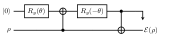
Denote as the channel which prepares the damped -qubit GHZ state from , combing all CNOTs and single-qubit damping channels into a single operator. We decompose this channel as follows:
| (15) | ||||
where and . For the random-unitary terms, we use the standard MQC technique Wei et al. (2020) as depicted in Figure 5, while absorbing any stochastically sampled gates into . After preparing , we apply the rotation operator , invert the preparation via , and then measure the all-zero population . For the following derivation, observe that . We thus measure the observable
| (16) | ||||
For the cross terms, the derivation is similar. In order to properly invert the preparation, we exactly mirror the preparation gates by re-applying any sampled damping gates and using the same ancilla qubits. Overall, this yields
| (17) | ||||
Combining these two schemes in the framework of SCU, in total we measure the all-zero population signal as
| (18) | ||||
Finally, by Fourier transforming the signals shown in Figure 2, we obtain the multiple-quantum intensity . The coherences are then , which we use to compute the fidelity relative to the ideal GHZ state.
In the Letter, we compare the experimentally measured fidelities with those of an ideal damped GHZ state, i.e. one hypothetically prepared on a noise-free quantum device. For these values, we use the following analytic calculations. The -qubit GHZ state preparation involves instances of CNOT-induced amplitude damping. As a result, the all-one population is reduced by a factor of , and the coherences are reduced by . Using these damped values in Eq. (4) gives an analytically predicted fidelity of .
I.2 Damped GHZ: Resource Analysis
In this section, we compare the resource costs of our SCU-based approach to the direct circuit implementation shown in Figure 6. Compared to previously proposed circuits for amplitude damping Rost et al. (2020), we designed this circuit to be CNOT-efficient to make a fairer comparison with our stochastic approach. In Table 1, we show that SCU requires a sampling overhead of per instance but has a reduced average CNOT cost of . SCU thus offers significant reductions in circuit depth, especially pronounced for weak damping parameters . As an example, consider our eight-qubit GHZ simulation with . For this case, the SCU approach requires a sampling overhead of . However, including damping in the eight-qubit MQC circuit uses 28 CNOT gates with the direct approach compared to an average of 1.27 CNOT gates with SCU. Thus, with minimal sampling overhead, our SCU-based approach reduces these gate costs by over an order of magnitude.
For strong damping parameters , the average CNOT cost with SCU is at most 1, still an improvement over the direct circuit. However, as the sampling overhead per instance increases, the scalability of this method suffers and eventually becomes impractical. In general, we recommend researchers balance this trade-off between depth reductions and sampling overhead for their specific applications.
| Method | Overhead | |
|---|---|---|
| Direct | ||
| Stochastic |
I.3 Markov Chain Sampling
In order for our SCU-based algorithms to be useful in early demonstrations of quantum advantage, we need to classically compute stochastic correction operators for reasonably large system sizes , i.e. approaching 100 qubits. With this goal in mind, here we limit our truncation order to at most ; this is merely a heuristic choice with which we can quickly compute corrections up to qubits on our 2023 personal computers. However, by borrowing ideas from Markov chains, we can use even higher-order operators without the need to fully expand and simplify them.
As an example, product formula remainder expressions can contain operators of the form and . For reasonably large , we can use Pauli algebra to fully compute second-order terms like or even fourth-order terms like . In contrast, seventh-order terms such as quickly become too costly to expand in the same way. We propose partitioning such terms into multiple layers of sampling, which in aggregate approximate the full operator. For this case, we 1) separately expand and , 2) sample each as independent ensembles and , and 3) approximate as the product of sampled operators . This yields an unbiased estimator but generally increases the norm compared to full expansion.
For the enhanced second-order product formula, this structure-agnostic approach allows us to achieve a spectral error corresponding to truncation order while still managing to empirically compute the overhead bounds up to 50 qubits. The downside is that we miss out on potential simplifications between the various remainder terms, ultimately increasing the sampling overhead. For example, applying this scheme to all remainders of the first-order product formula would effectively ignore the commutator scaling of the second-order correction, causing the normalization constant to scale worse with respect to system size.
I.4 Transverse Field Ising Model: Resource Analysis
After computing the number of time steps , we convert to CNOT cost. For the standard product formulas, we simply multiply the number of two-qubit Pauli exponentials by a factor of two. For qDRIFT, we multiply the total number of gates by the probability of sampling a two-qubit Pauli exponential, again rescaling this by a factor of two. For the enhanced product formulas, the dominantly sampled operators are the standard product formulas . For a time step , the probability of sampling is , and the probability of sampling first for the left operator and then for the right operator is . The probability of any other event is thus . Over all time steps , the expected number of sampled terms other than the standard product formula is simply
| (19) |
Asymptotically, for large r, we obtain
| (20) |
We conclude that the gate cost per time step is negligibly increased compared to the standard product formula approach.

For CTS, the dominantly sampled gates will be Pauli exponentials from , and the sampled left and right gates will typically differ. For the TFIM with , approximately half of the sampled gates will be and the other half will be . A controlled single-qubit Pauli exponential is locally equivalent to , which compiles to two CNOT gates. As shown in Figure 7, a controlled two-qubit Pauli exponential can be implemented with four CNOT gates. Thus on average, CTS uses approximately six CNOT gates per time step.
To minimize the need for ancilla qubits, one can use mid-circuit measurements, repeatedly resetting and reusing the same physical qubits. In principle, this approach requires only a single ancilla qubit for the entire simulation. Depending on the device capabilities, however, such measurements could create a bottleneck; a practical solution is to use a pool of ancilla qubits, thus lowering the frequency of measurements per individual qubit.
I.5 Proof of Theorem 1
First, we Taylor expand and separate the terms into real and imaginary subsets.
| (21) | ||||
Now substitute the following Pauli decompositions of each sum:
| (22) | ||||
Because all powers of are Hermitian, the coefficients are strictly real. We absorb any negative signs into the operators , and normalize by the norms and . This ensures that , thus creating convex sums of unitaries. Continuing, we get:
| (23) | ||||
In the final step, we use the substitution , where . This step was inspired by the excellent work of Wan et. al. (Wan et al., 2022, Appendix C). Finally, to prove the upper bounds on the norms, notice that and . Because , we conclude that and .
I.6 Worst-Case Complexity Analysis
Consider a general quantum channel , with the following Kraus decomposition:
| (24) |
Any Kraus operator can be written as a linear combination of unitary matrices, . For instance, the Pauli strings form an orthonormal basis of operators. Then, we obtain:
| (25) |
Theorem 2: Suppose that each of the Kraus operators decomposes into unitaries , and that . Then, the sampling norm of the coefficients in Equation 25 is at most .
Proof: First, we directly compute the norm of the coefficients in Equation 25:
| (26) | ||||
Now, use the property that is trace-preserving, i.e. :
| (27) | ||||
Thus, the second sum must be , but more importantly,
| (28) |
In other words, the norm of the set is . According to the Cauchy-Schwarz inequality, for complex numbers and ,
| (29) |
Setting , we obtain the following identity:
| (30) |
This is exactly what we need – by knowing the norm, we can set an upper limit on the norm. For our application, we set to obtain the following inequality, valid for all :
| (31) |
Thus,
| (32) |
Because the norm is 1, we get our final result:
| (33) |