∎
22email: emmanuel.gobet@polytechnique.edu 33institutetext: J. G. López-Salas (✉ Corresponding author, 33email: jose.lsalas@udc.es) 44institutetext: Centre de Mathématiques Appliquées, École Polytechnique and CNRS, route de Saclay, 91128 Palaiseau cedex, France 55institutetext: C. Vázquez 66institutetext: Department of Mathematics, Faculty of Informatics, Universidade da Coruña, Campus de Elviña s/n, 15071, A Coruña, Spain
66email: carlosv@udc.es
Quasi-Regression Monte-Carlo scheme for semi-linear PDEs and BSDEs with large scale parallelization on GPUs††thanks: The first author research is part of the Finance for Energy Markets (FiME) lab, of the Chair Financial Risks of the Risk Foundation and of the ANR project CAESARS (ANR-15-CE05-0024). The second author has been financially supported by the Chair Financial Risks of the Risk Foundation, the Spanish grant MTM2016-76497-R and the Xunta de Galicia 2018 postdoctoral grant. The third author was partially supported by Spanish grant MTM2016-76497-R.
Abstract
In this article we design a novel quasi-regression Monte Carlo algorithm in order to approximate the solution of discrete time backward stochastic differential equations (BSDEs), and we analyze the convergence of the proposed method. The algorithm also approximates the solution to the related semi-linear parabolic partial differential equation (PDE) obtained through the well known Feynman-Kac representation. For the sake of enriching the algorithm with high order convergence a weighted approximation of the solution is computed and appropriate conditions on the parameters of the method are inferred. With the challenge of tackling problems in high dimensions we propose suitable projections of the solution and efficient parallelizations of the algorithm taking advantage of powerful many core processors such as graphics processing units (GPUs).
Keywords:
BSDEs semi-linear PDEs dynamic programming equations empirical regressions parallel computing GPUs CUDAMSC:
49L20 62Jxx 65C30 93E24 68W101 Introduction
Since the 1940s, Feynman-Kac formula has provided a probabilistic interpretation of the solutions of linear partial differential equations (PDEs). Thence, Monte Carlo method has become an alternative to deterministic numerical algorithms for solving linear PDEs. While traditional deterministic methods like finite differences, finite elements or finite volumes suffer from the so-called curse of dimensionality bellmann (i.e. as the dimension grows, the complexity of the algorithms needed to achieve a given accuracy grows exponentially), the rate of convergence of Monte Carlo methods does not depend on the dimension of the state space. As a consequence, in order to solve equations of dimension greater than or , the probabilistic approach often remains the only numerical method available.
In the 1990s, the theory of backward stochastic differential equations (BSDEs) provided a probabilistic interpretation for non-linear problems. BSDEs are stochastic differential equations (SDEs) for which a terminal condition is specified and their solutions are pairs of processes. Linear BSDEs were introduced by Bismut bis:73 in 1973 in order to study stochastic control problems and their connections with the Pontryagin maximum principle of optimality. A rigorous study of (non-linear) BSDEs was started by Pardoux and Peng in 1990, who proved in their seminal article pard:peng:90 the first well-posedness result for non-linear BSDEs, see also pard:peng:92 . These equations have the general form of
where , is a Brownian motion, the terminal condition is a random variable, and the solution is a pair of adapted processes . The first applications of BSDEs in finance were conducted by El Karoui, Peng and Quenez elka:peng:quen:97 in 1997. They applied BSDEs in a European option pricing problem, where the randomness of comes from a forward SDE (FSDE in short) in as follows,
the function models possible imperfections and restrictions when trading in the markets. Now the terminal condition of the BSDE is determined by the stochastic terminal value of the FSDE through some deterministic function . This system of SDEs, to which we will devote this article, is known as decoupled111Fully coupled FBSDEs have the general form forward-backward stochastic differential equation (FBSDE in short). It is also referred as Markovian BSDE, since the terminal condition of the BSDE and are random only through a Markov process.
After the already mentioned celebrated work of El Karoui, Peng and Quenez, the interest in BSDEs has increased, mainly due to the connection of these tools with stochastic control and PDEs, connection that will be stated clearly soon. Let us start with a rigorous definition of the problem at hand.
The problem.
In this work we are interested in numerically approximating the solution of a decoupled forward-backward stochastic differential equation
| (1.1) | ||||
| (1.2) |
The terminal is fixed. These equations are considered in a filtered probability space supporting a dimensional Brownian motion . The filtration is assumed to be the natural filtration of augmented with the -null sets. In this representation, is a -dimensional adapted continuous process (called the forward component), is a scalar adapted continuous process and is a -dimensional progressively measurable process. Consideration of multi-dimensional is quite straightforward and is discarded for the sake of simplicity. Regarding terminology, is called terminal condition and the driver. Under standard assumptions (like -integrability and Lipschitz regularity), there is a unique solution (see pard:rasc:14 for broad account on existence/uniqueness assumptions). Detailed hypotheses for the current study are exposed later.
Our aim in this article is to design a new numerical scheme for approximating the solution to the above BSDE. When is linear in , explicit representations are available (elka:peng:quen:97, , Theorem 1.1), which can be easily turned into simple and efficient Monte-Carlo algorithms. Our focus is thus more on the case of non-linear driver yielding non-linear equations.
Feynman-Kac representations.
Let us clearly show that FBSDEs are important tools in semi-linear PDEs and stochastic control theory. Denote by the infinitesimal generator of :
where ⊤ denotes the transpose operator. Consider the parabolic partial differential equation (PDE) of the form
| (1.3) |
Assuming that is smooth enough, the Itô formula leads to
Using the PDE (1.3) and noting , we get
therefore proving that the solution can be represented as
This is the well-known Feynman-Kac representation, making connection between semi-linear PDEs and BSDEs. One may prefer one or the other representations depending on the application at hand, on the numerical scheme to use, and on the theoretical estimates available (of probabilistic or PDE nature). As a consequence, solving numerically for any realization of or computing in the full space gives, in both cases, essentially access to the same solution. The above reasoning holds for Cauchy boundary conditions and parabolic PDEs as presented above, however extensions in the directions of various boundary conditions (Dirichlet, Neumann, free-boundary) or stationary problems (elliptic PDEs) are also available, see (pard:rasc:14, , Sections 3.8, 5.4, 5.6, 5.7 and 5.8) and references therein.
In view of (1.3), the link with stochastic control appears clearly, by analogy with the Hamilton-Jacobi-Bellman equation. Since the non-linearity in is related only to the first derivative of (the component), the underlying control problem is associated to a control in the drift only (not in the diffusion coefficient). See elka:peng:quen:97 ; elka:hama:mato:08 for some examples in finance.
Applications.
We now conclude the presentation of connection between BSDEs and PDEs by giving a broader overview of applications where these semi-linear PDEs come into play. We follow the presentation of (gobe:16, , Section 7.1), some examples can be found in (henr:81, , Chapter 2) and (smol:94, , Chapter 14).
- •
-
Ecology. In a region of the plane (), suppose the existence of 2 interacting species in the same environment and denote () the population density of the individuals of each species at a point of the space and at a time . These population densities obey to the system
(1.4) where the two Laplacian operators model the diffusive movement (as a Brownian motion) of each species. Note that the initial condition at can be turned into a terminal condition at as in our previous setting, this is just a simple time reversal .
The function plays the role of a growth rate of the population, describing the available local resources and interactions between the species: the case and corresponds to the predator-prey model, where the growth rate of the species 1 (prey) decreases in the case of high density of the species 2 (predator) and conversely for the growth rate of predators; the case and models symbiosis, where each species benefits from the other; and describes competition between species. This kind of model, introduced in the 30s by Fisher, Kolmogorov, Petrovsky and Piskunov, is discussed with extra references in shig:kawa:97 .
- •
-
Chemistry. Suppose that a container contains chemical compounds taking part in independent reactions. Denote the concentration of the -th compound and the temperature. Then their evolution follows the equations (in )
(1.5) where is the speed of the -th reaction and is the partial molar enthalpy of the -th compound. For more details, see gava:68 . For reaction-diffusion equations, see smol:94 .
- •
-
Neuroscience. The famous model of Hodgkin and Huxley is a set of equations describing the psychological phenomenon of signal transmission in the axon (nerve fiber), showing the dependences between electrical excitability and various chemical ion concentrations. The PDE system is of size , the first unknown represents the electric potential and the three other unknowns are chemical concentrations: the system writes for (linear neuron)
(1.6) for different positive constants and different functions . There also exists a simplification of this model, known as the FitzHugh-Nagumo model.
- •
-
Materials physics. The Allen-Cahn equation is a prototype model of phase transition with a diffusive interface, used to model, for example, a solid/liquid phase transition visi:96 . The system is one-dimensional, and takes the form (in )
(1.7) The solution thus represents an order parameter defining the arrangement of atoms in a crystal lattice.
- •
-
Economy and finance. There are numerous applications of BSDEs (and semi-linear PDEs) in finance, we refer the reader to cvit:ma:96 ; elka:peng:quen:97 ; crep:13 . Let us mention: valuation/hedging of contingent claim in complete markets; some market imperfections, such as higher interest rate for borrowing berg:95 ; incomplete markets pham:09 or super-replication elka:quen:95 ; connections with recursive utilities in duff:epst:92 ; non-linear pricing rule peng:03:a ; second order BSDEs (2BSDEs) cheri:mete:touz:vict:2006 ; soner:touz:zhang:2011 which provide a stochastic representation for solutions of fully non-linear parabolic PDEs through a driver depending also on another process directly connected with the Hessian of the solution of the corresponding PDE; reflected BSDEs, where the solution is constrained to stay above a given process called obstacle, were introduced by El Karoui et al in karoui:kapo:pard:peng:quen97 , and combined with jumps are able to connect with partial-integro differential equations barles:buck:pard:97 ; delong:13 , etc. See elka:hama:mato:08 ; crep:13 for extra references of applications in finance.
Numerical approximations.
In the two past decades, there have been several attempts to design efficient approximation schemes for BSDEs. First, the four step algorithm was proposed by Ma, Proter and Yong ma:protter:yong:94 in 1994 to solve general FBSDEs. Their method is based on the finite difference approximation of the associated quasilinear parabolic PDE, and therefore becomes unaffordable in high dimension. In 1997, a discrete scheme based on the approximation of the Brownian motion by some discrete process was proposed by Chevance in chev:97 , while Bally considered a random time scheme in ball:97 , although this method requires the computation of conditional expectations to become a fully implementable solver. At that time, only time-discretization issue was considered. Since then, optimal discretization strategies have been derived: see geis:geis:gobe:12 and references therein. All probabilistic approaches proposed later roughly follow three steps: time discretization, dynamic programming principle and computation of conditional expectations. The problem of discretization and simulation of the forward component is well-understood, one could use standard Euler scheme or other choices like Milstein scheme, see kloeden:platen:92 . The difficulty lies in the backward component , since a naive discretization of the backward SDE in is not guaranteed to be adapted. In order to obtain a computationally viable backward induction scheme one should take conditional expectations. If the time grid is , it leads to a nested expectation problem of the form (also called Dynamic Programming Equation, or DPE for short)
| (1.8) | ||||
| (1.9) |
for . We use the symbol to emphasize the heuristics, a rigorous justification can be done using the aforementioned references. The scheme (1.8)-(1.9), which is known as one-step forward dynamic programming scheme, could be updated taking into account a resimulation of the forward process till terminal time , thus resulting in the so-called multi-step forward dynamic programming scheme, which is written as follows
| (1.10) | ||||
| (1.11) |
for .
Analytically, both schemes (1.8)-(1.9) and (1.10)-(1.11) are equivalent. However, differences arise when conditional expectations are numerically approximated. In fact, the multi-step scheme leads to better error estimates of the solutions computed by the developed algorithms, see bend:denk:07 ; gobe:turk:2016 . The above backward dynamic programming equations make clearly appear that at each of grid times, one has to compute a conditional expectation function, that is a function from to , this is in a way equivalent to solving the PDE at each time point . This is a difficult problem, with increasing difficulty as the dimension gets large and/or as the unknown function gets less smooth (curse of dimensionality), like for finite differences schemes for PDEs. Among the numerous approaches, let us mention the quantization method of Bally and Pagès ball:page:03 (and generalized to coupled FBSDEs by Delarue and Menozzi dela:meno:06 ; dela:meno:08 ), which is an optimal space discretization of the underlying dynamic programming equation, suitable to compute easily the conditional expectations on the space grid; in bouc:touz:04 the authors compute the regression function with Malliavin calculus integration by parts combined with Monte Carlo simulations; the use of empirical regression methods and machine learning techniques is developed in gobe:lemo:wari:05 ; lemo:gobe:wari:06 (also called regression Monte-Carlo method). Optimal convergence rates with regression methods are derived in gobe:turk:2016 , variance reduction using importance sampling is designed and analysed in bend:mose:10 ; gobe:turk:17 .
Recently, Henry-Labordere et al. henr:tan:touz:14 and Bouchard et al. bouc:tan:warin:zou:2017 proposed a branching method and a time step randomization applied to the Feynman-Kac representation of the PDE. Although branching techniques really overcome the curse of dimensionality, unfortunately they are only limited to small maturities, some small non-linearities and mainly to non-linearities that are polynomial in the solution and its gradient. Lately, in wei:jie:jentzen:2017 the authors propose a deep learning technique, referred as deep BSDE, to solve semi-linear PDEs or the corresponding BSDEs. They interpret the BSDE as a stochastic control problem with the gradient of the solution being the policy function, which is approximated or learned by a deep neural network, as has been done in deep reinforcement learning. More precisely, after discretizing the forward SDE in using Euler discretization, the algorithm reads the BSDE for as a forward SDE, and the method tries to learn the value of and at each time step of the Euler scheme by minimizing a global loss function between the forward simulation of until the maturity and the goal . In the recent work cwn:mik:warin:2019 , the authors give an improved version of the deep BSDE method, where a fixed point problem is solved using deep learning techniques. Numerical results show that these kind of algorithms are able to solve problems with some accuracy in dimension and even above. However, these methods suffer so far from the lack of rigorous error estimates and the matter that convergence is not guaranteed: as in linear regression methods gobe:turk:2016 , there must be a tricky interplay between the number of time steps, the number of simulations, the number of neurons and layers, to ensure a good accuracy. Moreover, one has to account for the likely possibility that the stochastic gradient descend method used to minimize the loss function is trapped in a local minimum.
Parallel computations.
Most of the above methods do not allow parallel computations because of the non-linearity of the equations. Recently in gltv , the authors have proposed a novel approach inspired from regression Monte-Carlo schemes suitable for massive parallelization, with excellent results on GPUs. It takes advantage of local approximations of the regression function in different strata of the state space (partitioning estimates) and of a new stratified sampling scheme to guarantee that enough simulations are available in each stratum to compute accurately the regression functions. The parallelization step is made with respect to the strata.
Our current work lies in this vein and is aimed at overcoming some drawbacks of the stratified regression scheme of gltv . In the previous scheme, the solution to the PDE is represented as a piecewise polynomial function (like in a discontinuous Galerkin method dipi:ern:11 ) and therefore, even if the exact solution is continuous, the approximation may be not, especially at the interface of the different strata. In the current work, we propose a different scheme, where the approximated solution is decomposed on basis functions that are smooth and that have natural orthonormal properties with respect to the sampling distribution, thus avoiding the possible discontinuity at the interfaces. Moreover, the sampling distribution is required to have some nice stability properties, useful for the propagation of error in the DPE , see Theorem 2.2; we prove that the Student’s t-distribution meets this requirement, see Theorem 2.1. One possible set of smooth and orthonormal functions is given by the trigonometric basis composed with a space transformation related to the Cumulative Distribution Function (CDF for short) of the Student’s t-distribution. We call such a basis the Student-cosine basis. Instead of a regression Monte Carlo scheme, we design a quasi-regression Monte-Carlo scheme: we take advantage of the fact that the basis functions enjoy orthonormal properties, in order to compute the basis coefficients as simple Monte-Carlo averages, instead of solutions of least-squares problems. On the one hand, it leads to a simplified and quicker procedure (because we avoid inverting linear systems). On the other hand, we obtain a globally smooth approximation which is mainly suitable for smooth solutions funaro ; Canuto-Hussaini-Quarteroni-Zang : this is a significant difference with partitioning estimates which can approximate well locally (ir-)regular functions. In this new scheme, the notion of strata is lost and the parallelization is now made with respect to the numerous required simulations and basis coefficients. Moreover, we establish tight non-asymptotic error estimates (as a function of the size of the function basis and the number of Monte-Carlo simulations).
In recent years, GPUs have become increasingly attractive for general purpose parallel computations. GPUs are not only impressive graphics tools but also highly parallel programmable processors that can deliver order-of-magnitude performance gains over optimized CPU applications. CPU hardware is designed to handle complex tasks, instead, GPUs only do one thing well, they handle millions of repetitive low level tasks. These high performance computing devices offer an arithmetic capability and a memory bandwidth that substantially outpace their CPU counterpart. In fact, a single NVIDIA Titan V GPU can sustain over 13.8 tera-floating-point operations per second (Tflops) and a memory bandwidth of 652.8 GB/s. In the last years GPUs have been heavily used in scientific computation in order to achieve dramatic runtime reductions over traditional CPU codes. Particularly successful applications of GPUs include Monte Carlo methods like the one we target in the present work. Indeed, Monte Carlo algorithms follow all design principles of GPU computing, they give rise to embarrassingly parallel not divergent codes that can exploit the GPU arithmetic intensity and its streaming memory bandwidth. In the last part of this article our goal is to offer an efficient implementation of the proposed algorithm taking advantage of several GPUs, which will allow us to address the solution of semi-linear PDEs in high dimensions.
Organization of the paper.
In Section 2, we set the framework of our study, define some notations used throughout the paper and describe our algorithm based on the approximation of conditional expectations by a projection on a finite orthonormal basis of functions. Compared to the usual DPE to solve (2.1), we propose an equivalent modification that includes a weighted factor: this weight is related to the sampling distribution and its crucial purpose is to lead to higher order approximation of the unknown function under the condition it is smooth (see the Fourier-based analysis in Section 2.4). Proofs of the propagation of error are postponed to Section 3.2. This new numerical scheme has been tested on GPU, which is exposed in Section 4. Numerical results are collected in Section 5.
Notations of the paper.
-
(i)
stands for the natural logarithm of .
-
(ii)
stands for the Euclidean norm of the vector .
-
(iii)
stands for the -norm of the vector , i.e.
. It will be mainly used when is a multi-index of integers used for differentiation. -
(iv)
means the positive part of defined by .
-
(v)
denotes the real part of the complex ; we set .
-
(vi)
For any finite and , define the soft truncation function
Moreover, if is a measurable function, then the above definition of is extended by replacing by :
(1.12) -
(vii)
Let , be two multi-indices. means that for all .
-
(viii)
The finite multi-indices set is downward closed if
-
(ix)
Let be an arbitrary downward closed multi-index set and . is -smooth if exist and are continuous for all .
2 Mathematical framework and basic properties
2.1 Model
2.1.1 Dynamic Programming Equation
From now on, we aim at solving the dynamic programming equation of the form (1.10)-(1.11). First, for the sake of simplicity, we intentionally consider the case where the non-linearity does not depend on the gradient (the component). Second, we consider the case of equidistant grid times of , i.e. we set with . Third, the forward component is approximated by an Euler scheme with time-step , see (2.6) below. These two last approximations are known to be accurate enough when data () are sufficiently regular (see geis:geis:gobe:12 for a precise statement). To simplify notation, we write and for an approximation of and .
All in all, our aim now is to solve
| (2.1) |
where , being the driver in (1.1). In other words, our subsequent scheme will approximate the solutions to
| (2.2) | ||||
and
| (2.3) |
Our assumptions on the functions are as follows.
-
is a polynomially bounded measurable function from to : there exist two finite non-negative constants and such that
For every , is a measurable function to , and there exist three finite non-negative constants such that, for every ,
-
The drift coefficient and the diffusion coefficient are bounded measurable functions.
One important observation is that, due to the Markov property of the Euler scheme, for every , there exist measurable deterministic functions , such that
almost surely. See the justification in (gobe:turk:2016, , Section 4.1). Moreover, we have an uniform absolute bound for the function , the proof is postponed in Section 3.3.
Proposition 1
Assume and . Then, for any and any , we have
| (2.4) |
with
| (2.5) |
A second crucial observation is that the value functions are independent of how we initialize the forward component. Our subsequent algorithm takes advantage of this observation. For instance, let be a random variable in with some distribution (more details on this to follow) and let be the Euler scheme evolution of starting from ; it writes
| (2.6) |
This flexibility property w.r.t. the initialization then writes
| (2.7) |
Approximating the solution to (2.1) is actually achieved by approximating the functions . In this way, we are directly approximating the solution to the semi-linear PDE (2.3). For some reasons that will appear clear later, we define a weighted modification of by
| (2.8) |
for a damping exponent . For , and coincide. The previous DPE (2.7) becomes
| (2.9) | ||||
The introduction of the polynomial factor gives higher flexibility in the error analysis, it ensures that decreases faster at infinity, which will provide nicer estimates on the approximation error when dealing with Fourier-basis, see Section 2.4.
2.1.2 Randomizing the initial value
For the subsequent algorithm, will be sampled randomly according to the distribution , which we list the properties below.
-
The distribution of has a density with respect to the Lebesgue measure on , of the form
(2.10) for some probability density functions , which are assumed to be strictly positive.
The function (where is defined in (2.4)) is square-integrable on with respect to .
We denote by the cumulative distribution function (CDF) of the one-dimensional marginal of ,and by its inverse (which is standardly defined since is continuous and strictly increasing).
Note that the above integrability condition ensures that (for any ) is square integrable on with respect to .
In this work, we deal essentially with one type of distribution.
Example 1 (Student’s t-distribution)
We deal with the non-standardized Student’s t-distribution on with parameter defined by its probability density function of the form (2.10) with
| (2.11) |
where . This is the density of where is a standard Student’s t-distribution with degrees of freedom. It leads to numerous ways to simulate , as acceptance rejection or ratio-of-uniforms methods, for example. From (jackman:2009, , p. 507) we know that
where is the Gamma function defined in (jackman:2009, , p. 501). Note that the marginal CDF and its inverse are not explicit in general for the Student’s t-distribution, however their values (for usual parameter ) are tabulated in most of books in statistics and computable using standard software libraries. Moreover, a priori estimates on , and , which will be used in the error analysis of the algorithm, are computed in the Appendix A.
Note that the square integrability of (see Assumption ) is guaranteed by the condition .
The distribution we have considered so far has mean zero, this is suitable for problems where 0 has a natural interpretation as the center in the application at hand. In order to solve the problem far away from the neighborhood of zero we should allow non zero means (say ): this is easy to handle by shifting the above distribution by . For instance, in the case of the Student’s t-distribution (Example 1), we would take
| (2.12) |
Since this centering adjustment is quite obvious, we mainly discuss the case of Example 1 in what follows.
More importantly, the probability measure is expected to satisfy another assumption stated below.
-
(depending on , , , , ) such that for any measurable function with , any , we have
(2.13)
This is a stability property about expectation of weighted functionals of the Markov chain . This property will be crucial for analyzing the propagation of error in the quasi-regression scheme (see the proof in Section 3.2). We now illustrate this property in relation with previous Example 1, the proof is postponed to Section 3.1.
Theorem 2.1 (Norm-stability)
Assume that is the Euler scheme (2.6) with time step of a SDE (2.2) which drift coefficient is bounded measurable, and which diffusion coefficient is bounded measurable and -Hölder continuous in space uniformly in time (for some ,
In addition, we assume that fulfills a uniform ellipticity condition:
Let be sampled from distribution in the case of Student’s t-distribution (Example 1): then holds for any .
2.2 Approximation spaces and basis functions
The aim of this section is to define some proper basis functions which satisfy orthogonality properties in and which span some space, see Proposition 2. It turns out that the choice of measure for defining the space has to coincide with the sampling measure of defined in : this plays an important role for designing Algorithm 1. Our strategy for defining such basis functions is to start from trigonometric basis on and then to apply appropriate changes of variable: later, this transform will allow to easily quantify the approximation error when truncating the basis, see Propositions 3 and 4.
Notation.
We start by setting notations to deal with appropriate space on or .
-
(i)
Let be a probability density satisfying . We will consider the space of measurable functions
In these spaces we define the inner products,
and the norms,
Before the general multidimensional case, we start with an easy computation in dimension 1.
Lemma 1 (Orthonormal basis functions in dimension 1)
Assume that satisfies in dimension . Let and . The basis functions
| (2.14) |
are orthonormal in with respect to the probability density weight .
Proof
Let . It is sufficient to see that
where we have used the change of variable . Clearly the cosine basis functions
| (2.15) |
are orthonormal in with respect to the Lebesgue measure, therefore .∎
Note that and . This change of variable will be useful in order to analyze the truncation error of series in terms of the truncation error of Fourier cosine series (see Section 2.4).
Now that the reader gets acquainted with the one-dimensional case, we move to the more general result for any dimension . First, the natural way to build an orthonormal multidimensional set of basis functions is to take tensor products of orthonormal one-dimensional basis functions. To this end we need to add the superscript to the notations of the basis functions in dimension 1. Therefore, from now on, and stand for the one-dimensional basis functions (2.14) and (2.15) in the -th coordinate, respectively. For any multiindex , set
| (2.16) | ||||
| (2.17) |
The transformation function and its inverse are defined by
Therefore, from the above and from (2.16)-(2.17), we readily check the relations
| (2.18) | ||||
| (2.19) |
To analyze orthogonality properties, we repeatedly use the following lemma, which proof is quite straightforward and left to the reader (use the same change-of-variable arguments as in the proof of Lemma 1).
Lemma 2
Assume satisfies . Then, for all functions , we have the following identities
As a consequence of Lemma 2 and Equality (2.19), since the tensored cosine functions are orthonormal in with respect to the Lebesgue measure, it implies that are orthonormal in with respect to the probability measure . Moreover, the cosine functions form a complete family in : this is a standard result in Fourier analysis (observe that here, the sine functions are not needed to get a complete basis since the scalar product is defined on and not ). We summarize our findings in a proposition ready to be used.
Proposition 2
Assume satisfies . The family of functions forms a complete orthonomal basis of with respect to the measure .
2.3 Global Quasi-Regression algorithm and convergence results
We now describe our main algorithm which is able to compute accurately the function defined in (2.9). For this, define
| (2.20) | ||||
which allows us to rewrite the exact solution as
Note that it is easy to justify that is square-integrable under , and (remind of the bound (2.4) and the integrability condition in ). Therefore, the exact solution is in , and consequently (Proposition 2) it can be decomposed in its series:
| (2.21) |
for some coefficients . In practice, the coefficients are computed only in a finite set of multi-indices . Different choices of are discussed later in Section 2.4.2.
The orthonormality property of the ’s (Proposition 2) combined with (2.21) yields
| (2.22) |
Thus, using the tower property of conditional expectation, we obtain, ,
| (2.23) |
The above expectations in (2.23) can be computed using Monte-Carlo simulations and evaluations of along different sampled paths . Since depends on the unknown solution, we have to replace it by approximations, using previous steps in the dynamic programming equation (2.9). It gives rise to the following Algorithm 1, which we will call Global Quasi-Regression Multistep-forward Dynamical Programming (GQRMDP) algorithm. To maintain good integrability properties along the iteration, we use the truncation function (1.12) with the upper bound (2.4).
Algorithm 1 (GQRMDP algorithm)
- Initialization.
-
Set .
- Backward iteration for to ,
-
(2.24) where for all ,
(2.25) and
(2.26)
In the algorithm, in order to compute we have considered independent copies of
which form a cloud of simulations We assume that the clouds of simulations are independently generated.
Our main result is the following error propagation theorem, which proof is postponed to Section 3.2.
Theorem 2.2
Assume , , and . Let be a multi-index and let be a finite set of multi-indices. Let be the basis functions defined in (2.18), as an orthonormal basis in , and let be the related Christoffel number neva:86 restricted to :
| (2.27) |
For each , define the following local error term
| (2.28) |
There is a finite positive constant (depending on model parameters but not on ) such that
Observe that provided that remains bounded, the constant can be taken as uniform w.r.t. the algorithm parameters. This is the situation in practice since for getting accurate approximations, we need to be small.
2.4 Truncation error for the Student-cosine basis
From Equations (2.21)-(2.22) and Lemma 2 we recall that where
| (2.29) |
Define the truncation of the -series of by
Therefore, from orthonormal properties of the basis functions, we have
In other words, are the Fourier coefficients of the projection of
| (2.30) |
over cosine basis functions. In the following section we will take advantage of this property to derive a tight bound for the truncation error , using assumptions on and its derivatives only (and not on ). The specific choice of the Student’s t-distribution measure of Example 1 plays an important role to get tractable conditions.
Now our aim is twofold. Firstly we prove that if is times () continuously differentiable on , with (for some ),
and if the parameters are such that
then the truncation error is controlled as
for some constant . In the following, we first establish the above result in dimension 1 (Proposition 3) and then in dimension (Proposition 4) .
Our second goal is improving this result when mixed derivatives of are also supposed smooth. Thus, we prove that if is -smooth, where , with (for some ),
and if the parameters are such that
then the truncation error satisfies the tail inequality
for some constant (Proposition 5).
2.4.1 One-dimensional case
In this section, we let be the Student density (2.11).
Lemma 3
Assume that is times () continuously differentiable on , with the existence of a polynomial growth degree such that
| (2.31) |
Assume the relation
| (2.32) |
between , , the Student parameter and the damping exponent . Then is times continuously differentiable on , and its first derivatives vanish at and :
Proof
The regularities of and are straightforward in view of (2.8)-(2.30) and Lemma 15. The estimate is clearly true since it is equivalent to , which holds owing to the condition .
From now on, we may consider the case and . We start showing that for ,
| (2.33) |
In fact, using Leibniz rule,
Besides,
which leads directly to the desired result (2.33).
We now estimate . In order to compute the -th derivative of we take advantage of the following Faà di Bruno’s formula (Johnson02thecurious, , pp. 224–226),
| (2.34) |
As , using also (A.7),
| (2.35) |
The above bound goes to 0 as since .
Analogously, as , we have
| (2.36) |
which converges to 0 as since . ∎
Lemma 4
Proof
The integrability of on any compact set of the form () is obvious owing to the continuity of the function to integrate. As a consequence one has only to consider what happens around 0 and 1. As we have just seen in the proof of Lemma 3 (see (2.35)-(2.36)),
therefore it is square-integrable around and provided that
. Since the condition (2.37) is sufficient.
∎
Proposition 3
Proof
Under (2.37), we can invoke Lemma 3 (with derivatives) and Lemma 4 (with derivatives), to get
| (2.39) |
The coefficients coincide with the Fourier coefficients of the decomposition of with respect to the orthonormal basis functions in (see the relations (2.29)-(2.30)). The -cosine series of writes
where
Applying integration by parts ( is continuously differentiable) and using that
we get (for )
| (2.40) |
Thanks to (2.62), we can repeat times the integration by parts as above, and we obtain
| (2.41) |
Observe that the sets
and
are made of orthonormal functions in . Consequently, for any value of , is a set of orthonormal functions and the equality (2.4.1) means that are the projection coefficients of on these orthonormal functions. As such, the Bessel inequality gives
It readily follows
∎
2.4.2 Multi-indices sets
In this work only arbitrary downward closed multi-indices sets are considered. As already stated in the introduction, the finite multi-indices set is downward closed if
where means that for all . The most well-known of such multi-indices sets is the full or tensor product multi-indices set. For any where for all , the full anisotropic multi-indices set and its complement are defined by
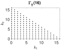
In high dimensions the full multi-indices set suffers from the curse of dimensionality. In order to effectively compute the projection of over a multidimensional set of of basis functions we propose to consider the following two sparse sets of downward closed multi-indices sets, where denotes a nonnegative integer:
-
•
Total degree set defined by
where .
-
•
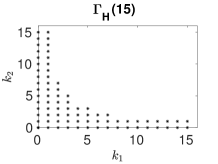
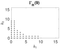
Hyperbolic cross index set defined by
In order to compute the number of elements in we split this set in the following two disjoint sets:
-
–
-
–
On the one hand, let us compute . Firstly we define
Secondly we divide in the following disjoint sets,
For any integer having the prime factorization
is equal to the number of possible ways to write as a product of exactly of its factors,
Therefore,
On the other hand, let us compute . Firstly we define as the subset of containing the multi-indices of with exactly of the indexes equal to zero, . Note that . Therefore, since
Finally, we conclude using that
-
–
2.4.3 Multidimensional case
In this section, we let be the Student density (2.10)-(2.11) in dimension . In the first part of the section only and its coordinate-wise derivatives are assumed to be smooth. In the second part, on top of that mixed derivatives of will be supposed smooth. Let us start with the first case.
Lemma 5
Assume that is times () coordinate-wise continuously differentiable on , with the existence of a polynomial growth degree such that
| (2.42) |
Assume the relation
| (2.43) |
between , , the Student parameter and the damping exponent . Then is times continuously differentiable on , and its first coordinate-wise derivatives vanish at :
Proof
As in dimension 1, the regularities of and are straightforward to obtain.
The statement is clear since the limit coincides with that of
as , which equals to 0 in view of . Therefore, from now on, we may consider and let be fixed.
In the following, to deal with comparison of functions as tends to , we use the same notation for any generic constants, that do not depend on , but that may depend on the order of derivatives under consideration. We will keep the same from line to line, in order the alleviate the computations, although its value changes.
We start by showing that for ,
| (2.44) |
By applying the Leibniz rule to the product (2.8) (as in dimension 1, since we differentiate times with respect to the same variable ) we get
| (2.45) |
Our standing assumptions write
| (2.46) |
From (A.2) we know that
By plugging the previous upper bound and (2.46) into the Leibniz formula (2.45), we get
we are done with (2.44).
Lemma 6
Proof
In view of the bound (2.47), it is sufficient to check the integrability on of
Observe that the function is symmetric with respect to each hyperplan , . Therefore, only the integrability on has to be established, which is equivalent to prove
Use the change of variables , then the above integral writes (up to a non-zero factor)
where is given by . To show that , we may decrease as much as needed to get . Once done, using the inequality
available for any , it yields (by direct induction) the existence of a constant such that
for any . Consequently,
We are done. ∎
Proposition 4
Proof
By definition of , we have the union bound
therefore the advertised inequality (2.49) directly follows from
| (2.50) |
We only prove the case , the arguments apply similarly for other .
Under (2.48), we can invoke Lemma 5 (with derivatives) and Lemma 6 (with derivatives), to get
| (2.51) |
In view of (2.29)-(2.30), the Fourier coefficients of the decomposition of with respect to the orthonormal basis functions in are given by n and the -cosine series of writes
where
Applying integration by parts in ( is uniformly bounded on , continuously differentiable and the derivative with respect to is integrable) and using that , we get for
Thanks to (2.51), we can repeat times the integration by parts as above, and we obtain
| (2.52) |
Observe that the sets
are made of orthonormal functions in . Consequently,
is (for any value of ) a set of orthonormal functions and the equality (2.4.3) means that are the projection coefficients of on these orthonormal functions. As such, the Bessel inequality gives
It readily follows
The proof of (2.50) is now finished and Proposition 4 is proved. ∎
Now we consider that not only and its coordinate-wise derivatives are smooth but also its mixed derivatives.
Lemma 7
Let be an arbitrary downward closed multi-index set and set . Assume that is -smooth with the existence of a polynomial growth degree such that
| (2.53) |
Assume the relation
| (2.54) |
between , , the Student parameter and the damping exponent . Then is -smooth on and its derivatives vanish at :
Proof
We start by showing that for , ,
| (2.55) |
By applying the multivariate Leibniz rule to the product (2.8) we get
| (2.56) |
Our standing assumptions write
| (2.57) |
From (A.4) we know that
By plugging the previous upper bound and (2.57) into the Leibniz formula (2.56), we get
we are done with (2.55).
Let denotes a list. In order to compute the (, ) derivative of we take advantage of the multivariate Faà di Bruno’s formula derived from (constantine:savits:96, , Theorem 2.1):
Combining the above with Lemma 11 and the estimates (A.7), we obtain
| (2.58) | |||
| (2.59) |
Since , we get that . ∎
Lemma 8
Proof
The proof follows readily from the proof of Lemma 6 by replacing by .
Proposition 5
Proof
Under (2.60), we can invoke Lemma 7 (with derivatives) (condition ) and Lemma 8 (with derivatives) (condition ), to get
| (2.62) |
By doing integration by parts on the Fourier coefficients of as we have already done in Proposition 4 we readily obtain
| (2.63) |
where is the -th antiderivative of such that
Equation (2.63) tells us that is a function in a Korobov space (krommerUeberhuber:94, , Definition 6.5.6, p. 225). Observe that the sets
are made of orthonormal functions in . Consequently,
is (for any value of ) a set of orthonormal functions and the equality (2.63) means that are the projection coefficients of on these orthonormal functions. As such, the Bessel inequality gives
It readily follows
∎
Equation (2.63) means that the most significant coefficients are the ones for which the product is as small as possible. Under this setting we prefer to consider the hyperbolic cross index set (Proposition 5) rather than the total degree set (Proposition 4). In fact, although the hyperbolic truncation error with will be greater than the total truncation error with , if belongs to a Korobov space, the hyperbolic truncation error will be near to the total truncation error (here we are assuming that is big enough to take into account all the significant Fourier coefficients). Besides, having in mind that (specially in high dimensions), the statistical error, driven by , will be smaller for the hyperbolic multi-indices set, considering the same number of simulations . Last but not least, the algorithm executed with the hyperbolic multi-indices set will be less time consuming than with the total degree set. This behavior is shown in the numerical experiments of Section 5.
3 Proofs related to error analysis
3.1 Proof of Theorem 2.1
First observe that we can restrict in the proof of (2.13) to the case of bounded measurable functions : indeed, for (possibly unbounded), apply the inequality (2.13) to the bounded function where to get (for any )
| (3.1) |
and take the limit . On the one hand, the dominated convergence theorem (because ) ensures that the r.h.s. of (3.1) converges to . On the other hand, by Fatou’s lemma, the liminf of the l.h.s. of (3.1) is bounded from below by , which all in all, gives the result (2.13) for the square integrable function .
Now we establish (2.13) for bounded functions . We follow and adapt the arguments of (gobe:turk:17, , Proposition 3.1 and Proposition 3.3 item (b)) which paves the way for (although the distribution is different). Under the current assumptions on and , the Euler scheme is a non-homogeneous Markov chain which transition kernel has a probability density w.r.t. the Lebesgue measure on . This density is denoted by where stands for the time indices and (resp. ) stands for the initial (resp. final) space point. This probability density satisfies to a Gaussian upper bound of Aronson type (see (lema:meno:10, , Theorem 2.1)): there is a finite constant (depending on , , , , but not on ) such that
| (3.2) |
for any and any . Assume that is such that, for any , there is a finite constant (depending on and ) such that, for any and any , we have
| (3.3) |
Then we claim that the inequality (2.13) holds, still considering bounded (which clearly ensures that both sides of (2.13) are finite). Indeed, combining (3.2) and (3.3), we get
| (use (3.2) and the change of variable ) | ||||
which gives the announced result (2.13) with .
Therefore, it remains to establish (3.3); since
for getting (3.3) it is enough to prove (for any )
| (3.4) |
Set . Denote by (resp. ) the above integral restricted to (resp. ). On , use that to obtain
Split each integral according to the set and use the bound : it gives
where is the cumulative density function of the standard normal distribution, where is a finite positive constant depending only on and , and where at the last line, we have used that is decreasing when faster than any polynomial. Therefore, we have proved
| (3.5) |
Now we deal with , i.e. the part of the integral of (3.4) restricted to . On this set, , therefore we obtain
| (3.6) |
where the last inequality follows from usual comparisons between exponential and polynomial growth. Gathering (3.5) and (3.6) gives the announced estimate (3.4) for some constant . Theorem 2.1 is proved. ∎
3.2 Proof of Theorem 2.2
In all this section, we assume the assumptions of Theorem 2.2 are in force, without further reference.
In addition to the coefficients calculated with the responses computed using the erroneous functions (see the definitions (2.24) and (2.25)), we define the following coefficients calculated with the responses computed with the exact functions ,
| (3.7) |
and thus
| (3.8) |
3.2.1 Preliminary results
The next result states a decomposition of the local error as a superposition of an approximation error (truncation over the functions basis) and a statistical error.
Lemma 9 (Bias/variance decomposition)
Proof
By definition of and ,
By orthonormality of the we obtain
For , observe that , therefore
which leads to the desired result. ∎
Before stating the next preliminary result we define the following -algebras generated by the cloud of simulations,
Lemma 10
We have
| (3.9) | ||||
| (3.10) |
Proof
We start with the proof of (3.9). Let be the projection coefficients in of the function
over the functions . Since the latter form an orthonormal basis of (Proposition 2) and owing to the tower property of conditional expectation, we have
| (3.11) |
By the Parseval identity and the Jensen inequality, we get
By recalling the representation (3.11) for , the above inequality readily leads to (3.9).
3.2.2 Proof of Theorem 2.2
Let . By definition of , and ,
Then, using the triangular inequality for norm and the inequality , we obtain
| (3.12) |
The first term is bounded taking into account Lemma 9:
| (3.13) |
Regarding the second term , the orthonormality of gives
| (3.14) |
To handle write
and apply Lemma 10, thus obtaining
| (3.15) |
Now we focus on . We recall the conditional variance formula , available for any scalar random variable and any sigma-algebra : then,
We start with :
We continue with : use Lemma 10 to write
Summarizing the above computations, we get a bound for :
All in all, in view of (3.14)-(3.15) and the above, we have derived a bound on :
| (3.16) |
It remains to estimate the above term with the difference of the responses. Using the Cauchy-Schwarz inequality for the summation in , and taking into account that is Lipschitz in , we obtain
| using that and that is -Lipschitz (see Proposition 1 and Definition (1.12)) | ||||
Combine this with (3.16) to obtain,
Finally, taking advantage of the norm-stability property of the distribution (see (2.13)) we get,
| (3.17) |
Let us set . At this point, in view of (3.12), (3.13) and (3.17) we have obtained
Apply now (gt2016, , Proposition 2.4) with to get the existence of a constant (depending only on ) such that
We are done. ∎
3.3 Proof of Proposition 1
Without loss of generality, we can assume from now that because assumptions on and are still valid by choosing the maximum parameter between and . Set . First note that the constant in (2.5) is finite since and are bounded, this follows from standard manipulations which are left to the reader.
Second we prove (2.4) by induction on . It is obvious for since (note that ). Now assume that
| (3.18) |
for for some and for some finite ’s, and let us prove that the inequality holds also for . In the proof below, we will get a relation between the ’s leading to the statement of Proposition 1. We start from (2.7) and make use of the growth assumptions on , and the Lipschitz property of : we have
Therefore, (3.18) holds for too, and thus owing to the induction principle, it holds for any . Moreover, we can take
The Gronwall lemma implies that ∎
4 GPU implementations
Two implementations on GPUs of Algorithm 1 are proposed in this section. The first one is a parallelization of the algorithm on a single GPU, we will refer to it as the (mono-)GPU version. This version includes two kernels, one simulates the paths of the forward process and computes the associated responses, the other one computes the regression coefficients . In the first kernel the initial value of each simulated path of the forward process is stored in a device vector in global memory, it will be read later in the second kernel. In order to minimize the number of memory transactions and therefore maximize performance, all accesses to global memory have been implemented in a coalesced way. The random numbers needed for the path generation of the forward process were generated on the fly (inline generation) taking advantage of the NVIDIA cuRAND library ref:curand and the generator MRG32k3a proposed by L’Ecuyer in ecuyer:99 . Therefore, inside this kernel the random number generator is called as needed. Another approach would be the pre-generation of the random numbers in a separate previous kernel, storing them in GPU global memory and reading them back from this device memory in the next kernel. Both alternatives have advantages and drawbacks. In this work we have chosen inline generation having in mind that this option is faster and saves global memory. Besides, register swapping was not observed on the implementation and the quality of the obtained solutions is similar to the accuracy of pure sequential traditional CPU solutions achieved employing more complex random number generators. Additionally, the pre-generation of random numbers is not feasible when dealing with a huge number of simulations , as required for high dimensional problems, since it will require more memory than the available in the GPU. In the second kernel, in order to compute the regression coefficients, a parallelization not only over the multi-indices but also over the simulations was proposed. Thus, blocks of threads parallelize the outer for loop , whilst the threads inside each block carry out in parallel the inner loop traversing the vectors of the responses and the simulations. We stress that the parallel sum reduction (2.25) has been implemented in shared memory avoiding bank conflicts in pursuance of getting the most of the GPU.
A host can have several GPUs attached (in our machine, 4 GPUs TITAN BLACK). When dealing with high dimensional problems demanding a huge number of simulations it is compelling to harness the computing power of these extra GPUs to further reduce execution times. The approach we have followed is to use OpenMP ref:openmp to control all GPUs inside the host node. This strategy involves launching as many CPU threads as GPUs available on the node, so that each CPU thread handles one GPU. We will allude this version as M(ulti)GPU. In order to simulate the forward process and compute the responses, each GPU runs in parallel the first previous mono-GPU kernel, storing in its global memory the initial Student random variable of each path and the computed responses of the paths. Having done that, in order to compute the regression coefficients, the outer loop is executed sequentially in CPU, whereas the inner loop on the simulations is performed in parallel across all GPUs. More precisely, the parallel reduction operation is executed in two levels. The first reduction level is carried out inside each one of the GPUs, it has been performed using the reduce primitive of the NVIDIA Thrust library ref:thrust . The second level of reduction was made in the plane of CPU threads. This approach of parallelizing only over the simulations of the forward process behaves optimally when the number of simulations is large enough to fully occupy the GPU. In fact, this is the scenario we will be dealing with when tackling high dimensional problems. Actually, as sketched in Theorem 2.2, in order to get accurate approximations we need to be small, therefore one need to choose much bigger than . This fact motivates a small variant of this multi-GPU version, specifically designed for problems where is so large that we cannot store the initial values of the simulated paths in the set of global memories of the GPUs. In the first kernel in charge of simulating the paths of the forward process and computing the associated responses, now the initial values of the forward process at each time step are not stored, thus saving bytes of global memory222Single precision data type is assumed.. Instead, we just store the initial random seeds of the launched threads, which will be used in the next kernel in order to resimulate the same initial values of the forward process and allow the computation of the regression coefficients. This strategy is even as efficient as the previous one, on the grounds that GPUs are (most often) faster recomputing data than getting this data back from global memory. This is due to the fact that the version recomputing data is less memory bounded than the first one.
5 Numerical experiments
We introduce the following functions
We aim to solve the PDE:
| (5.1) | ||||
Note that
is solution to (5.1). The probabilistic formulation goes as follows:
Then, the processes satisfy and . For the numerical results the final time is fixed to 1, and .
The parameter of the Student’s t-distribution is chosen as . Under this choice . The marginal CDF and its inverse are given by
| (5.2) |
In order to sample according to , we draw independent random variables with uniform distribution on , and we compute
First we present some numerical results in dimension 1. Taking into account that
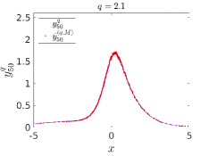
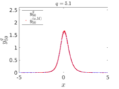
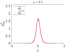
in order to fit the assumptions of Lemma 3 we select . The values of are selected using relation (2.37) under for and . Therefore, for only the function is square integrable; for the function and its first spatial derivative are square integrable and the function vanish for ; finally, for the function and its first two spatial derivatives are square integrable and vanish for , its third spatial derivative is square integrable, as well.
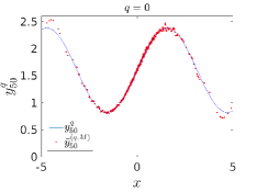
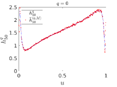
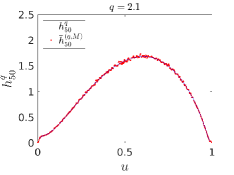
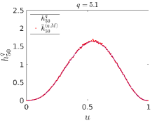
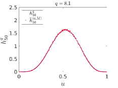
In Figure 2, the analytical solution versus the computed approximation are plotted for and the values of . The function was approximated on independent and identically distributed simulations. As long as increases the convergence of the algorithm is improved (the truncation error shrinks to 0, coherently with Proposition 3). In Figure 3 the corresponding results are presented for and ; for large the functions are very flat at the boundaries and , as expected. The parameters of the GQRMDP algorithm were chosen , meaning that was projected over basis functions, and . This selection makes small, in fact it is , thus we control well the statistical error of the algorithm.
In order to assess the performance of the algorithm, we compute the average mean squared error () over independent runs of the algorithm for two error indicators:
| (5.3) |
where the simulations are independent and identically -distributed, and independently drawn from the simulations used for the GQRMDP scheme.
In order to test the theoretical results we compare the performance of the algorithm according to the choice of the damping exponent and the multi-indices set. We will show the impact of these choices on the convergence of the approximation of the semi-linear PDE and on the computational performance in terms of computational time and memory consumption.
The numerical experiments have been performed with the following hardware and software configurations: four GPUs GeForce GTX TITAN Black with GBytes of global memory per device (see CUDA:keplerArchitecture for details in the architecture), two multicore Intel Xeon CPUs E5-2620 v2 clocked at GHz ( cores per socket) with GBytes of RAM, CentOS Linux, NVIDIA CUDA SDK 7.5 and INTEL C compiler 15.0.6. The CPU programs were optimized and parallelized using OpenMP ref:openmp . The multicore CPUs time (CPU) and the GPU time (GPU) will all be measured in seconds in the forthcoming tables. CPU times correspond to executions using threads so as to take advantage of Intel Hyperthreading. Unless otherwise indicated, the results are obtained using single precision, both in CPU and GPU.
All examples will be run using thread blocks, each with threads. In the following Table 2 we show results for and the choices of the damping exponent . As we have just seen in Figure 2, we expect (see Proposition 3) that the convergence of the algorithm is improved for large values of the damping exponent . Besides, as long as the time step decreases, our parameter choice is such that increases and decreases so that the algorithm is more and more accurate. The GPU implementation provides a significant reduction in the computational time: the GPU speed-up reaches the value . One usually expects a GPU speed-up factor between x-x vs two sockets of CPU VictorWLee , therefore both CPU and GPU codes were thoroughly optimized.
| CPU | GPU | |||||
|---|---|---|---|---|---|---|
In order to assess the accuracy of the proposed algorithm, in the following Table 3, for , and different values of , and , confidence intervals for are shown in the knowledge that . These confidence intervals were computed using 50 independent runs of the algorithm. Since we are computing the solution at the origin, similar results are obtained for values of .
Now we present results in dimensions greater than one, for which the total degree and the hyperbolic cross index sets are different. Coherently with Section 2.4.3, we start showing the behaviour of the algorithm when the discussed conditions are enforced only on coordinate-wise derivatives of . Table 4 shows results for . Convergence is clearly improved by increasing , considering (), not only and its first two coordinate-wise derivatives are square integrable but also and its first coordinate-wise derivatives vanish at the boundaries of . Additionally, convergence is enhanced as long as decreases: and the number of simulations increase in a way such that decreases. Finally, the hyperbolic cross index set offers better performance than the total degree set, not only an improved rate of convergence but also much faster computational times. In fact, for , the hyperbolic cross index set is not only almost times faster than the total degree set (on GPU), but also more accurate achieving instead of . The GPU speed-up with respect to a fully optimized CPU parallel version reaches the value .
| CPU | GPU | |||||||||
|---|---|---|---|---|---|---|---|---|---|---|
| Total | ||||||||||
| Hyper. | ||||||||||
Tables 5 and 6 show results for and , respectively. As before, the convergence of the algorithm improves for large values of the damping exponent, so that we benefit from small approximation error (see Proposition 4 with the conditions (2.43)-(2.48)). Furthermore, the hyperbolic cross index set outperforms the total degree set (which can be expected from the equation (2.63)). Except for the cases with , where there are not enough simulations to fully take advantage of four GPUs, the multi-GPU implementation provides a significant reduction in the computational time: the speed-up with respect to the mono-GPU version reaches the value . The ideal speed-up would be , although the multi-GPU parallelization introduces some overhead which makes this value unattainable.
| GPU | MGPU | |||||||||
|---|---|---|---|---|---|---|---|---|---|---|
| Total | ||||||||||
| Hyper. | ||||||||||
| MGPU | |||||||||
|---|---|---|---|---|---|---|---|---|---|
| Tot. | |||||||||
| Hyper. | |||||||||
Finally, results for , and are shown in Table 7 considering only the scenario performing better, i.e. the multi-GPU version considering a large value of the damping exponent along with the hyperbolic cross index set for the selection of the basis functions on which to project .
| MGPU | |||||||
|---|---|---|---|---|---|---|---|
Before the end of this section, the behavior of the algorithm is exhibited using larger values of the damping exponent that account for the case where not only coordinate-wise derivatives of but also its mixed derivatives are required to vanish at the boundaries of and to be square integrable. Taking into account that
and under , in order to fit the assumptions of Lemma 7 we select . In the following numerical experiments or will be selected. In order to avoid too large values of , which will hinder the computation of the damping factor when single and even double precision are considered, the parameter of the Student’s t-distribution is chosen as from now on. Under this choice we deal with the Cauchy distribution , whose CDF and its inverse are given by and , respectively.
Tables 8 and 9 show the behavior of the algorithm using a value of satisfying the condition (2.60) for , which boils down to in our benchmark scenario. As expected from equation (2.63) for the Fourier coefficients of , the hyperbolic cross index set clearly outperforms the total degree set. In order to take the most of our runtime environment, the codes were executed taking advantage of the whole available GPUs and the computations were performed using single precision.
| MGPU | |||||||
|---|---|---|---|---|---|---|---|
| Total | |||||||
| Hyper. | |||||||
| MGPU | |||||||
|---|---|---|---|---|---|---|---|
| Tot. | |||||||
| Hyper. | |||||||
Ultimately, the semi-linear PDE (5.1) is solved for dimension and in Table 10, and for dimension and in Table 11. The GQRMDP algorithm was executed using double precision and considering only the hyperbolic cross index set for the projection of . For , the so-discussed conditions are imposed for , while for , in order to avoid larger values of , these smoothness conditions are only forced for . The error indicators and the computational time for inside Table 10 are to be compared with those of Table 7: as it was anticipated, for the algorithm obtains much better convergence, whereas the execution time is larger due to more accurate computations on double precision.
| MGPU | ||||||||
|---|---|---|---|---|---|---|---|---|
| MGPU | ||||||||
|---|---|---|---|---|---|---|---|---|
Appendix A Appendix. Technical estimates on Student’s t-distribution
In this appendix, estimates on the CDF of the Student’s t-distribution, its inverse and the derivatives of the inverse of the CDF are computed. As we have been doing in the article, we use the same notation for any generic constants, we will keep the same from line to line, in order the alleviate the computations, although its value changes. In this appendix stands for Student’s t-distribution density (2.11) with parameter , its marginal CDF and its inverse.
Lemma 11 (Estimates on and )
Let , . The following estimates hold
| (A.1) | ||||
with
Proof
In view of (2.11) we know that . Besides,
The distribution being symmetric, we have and . Therefore, the estimate for follows from the case .
In order to compute we use that : If , , . Therefore,
which is the advertised result. The case follows from the case for using again the symmetry of the distribution . ∎
Lemma 12 (Estimates on derivatives of )
Let , and . The following upper bound holds
| (A.2) |
Proof
We only have to consider the case . In order to compute we use the following Faà di Bruno’s formula (as long as the partial derivative is only with respect to one variable we can extend in the following way the one-dimensional Faà di Bruno’s formula (2.34)):
| (A.3) | ||||
Here, consider and : and . Observe that in the Faà di Bruno’s formula (A.3), the sum over will be made only for with terms, and for with terms. Owing to this property and by definition of , we have and , which results in and . Invoking the form of the derivatives , it readily follows that
All in all, we deduce
∎
Lemma 13 (Estimates on derivatives of )
Let , , . The following upper bound holds
| (A.4) |
Proof
We only have to consider the case . For such , we use the following multivariate Faà di Bruno’s formula derived from (constantine:savits:96, , Corollary 2.10)
| (A.5) | ||||
where the positive constants depend on and the matrix under consideration.
Note that non coordinate-wise derivatives of are all zero. Besides, coordinate-wise derivatives of are . For a given , let denote the number of vectors in with in the -th coordinate and zero anywhere else. It holds that
for . All in all, we deduce
∎
Lemma 14 (Estimates on derivatives of Student’s t-distribution)
Let . The following upper bound holds
| (A.6) |
Proof
This result follows readily using the previous estimate (A.2). ∎
Lemma 15 (Estimates on derivatives of )
Let . The following upper bounds hold
| (A.7) |
where is a constant depending on and .
Proof
Using the combinatorial formula for higher derivatives of inverses Johnson02thecuriousInverse and the fact that for , , ,
Therefore, using (A.6),
Finally, combining the previous upper bound with (A.1) yields
where the constant may change value along computations. ∎
Compliance with Ethical Standards
-
•
Conflict of Interest: The authors declare that they have no conflict of interest.
References
- (1) Bally, V.: Approximation scheme for solutions of BSDE. In: Backward stochastic differential equations (Paris, 1995–1996), Pitman Res. Notes Math. Ser., vol. 364, pp. 177–191. Longman, Harlow (1997)
- (2) Bally, V., Pagès, G.: A quantization algorithm for solving multi-dimensional optimal stopping problems. Bernoulli 9(6), 1003–1049 (2003)
- (3) Barles, G., Buckdahn, R., Pardoux, E.: Backward stochastic differential equations and integral-partial differential equations. Stochastics and Stochastics Reports 60(1-2), 57–83 (1997)
- (4) Bellmann, R.: Adaptive control processes: A guided tour. Princenton University Press (1961)
- (5) Bender, C., Denk, R.: A forward scheme for backward SDEs. Stochastic Processes and their Applications 117(12), 1793–1823 (2007)
- (6) Bender, C., Moseler, T.: Importance sampling for backward SDEs. Stochastic Analysis and Applications 28(2), 226–253 (2010)
- (7) Bergman, Y.: Option pricing with differential interest rates. Rev. of Financial Studies 8(2), 475–500 (1995)
- (8) Bismut, J.M.: Conjugate convex functions in optimal stochastic control. Journal of Mathematical Analysis and Applications 44(2), 384–404 (1973)
- (9) Bouchard, B., Tan, X., Warin, X., Zou, Y.: Numerical approximation of BSDEs using local polynomial drivers and branching processes. Monte Carlo Methods and Applications 23(4), 241–263 (2017)
- (10) Bouchard, B., Touzi, N.: Discrete time approximation and Monte-Carlo simulation of backward stochastic differential equations. Stochastic Processes and their Applications 111, 175–206 (2004)
- (11) Canuto, C., Hussaini, M.Y., Quarteroni, A., Zang, T.A.: Spectral Methods, Fundamentals in Single Domains. Springer, Berlin (2006)
- (12) Chan-Wai-Nam, Q., Mikael, J., Warin, X.: Machine learning for semi linear PDEs. Journal of Scientific Computing pp. 1–46 (2019)
- (13) Cheridito, P., Soner, H.M., Touzi, N., Victoir, N.: Second-order backward stochastic differential equations and fully nonlinear parabolic PDEs. Communications on Pure and Applied Mathematics 60(7), 1081–1110 (2007)
- (14) Chevance, D.: Numerical methods for backward stochastic differential equations. In: Numerical methods in finance, Publ. Newton Inst., pp. 232–244. Cambridge Univ. Press, Cambridge (1997)
- (15) Constantine, G.M., Savits, T.H.: A multivariate Faa di Bruno formula with applications. Transactions of the American Mathematical Society 348(2), 503–520 (1996)
- (16) Crepey, S.: Financial modeling: a Backward Stochastic Differential Equations perspective. Springer. Springer-Verlag, Berlin (2013)
- (17) NVIDIA cuRAND web page: https://developer.nvidia.com/curand
- (18) Cvitanic, J., Ma, J.: Hedging options for a large investor and Forward-Backward SDEs. The Annals of Applied Probability 6(2), 370–398 (1996)
- (19) Delarue, F., Menozzi, S.: A forward backward algorithm for quasi-linear PDEs. Annals of Applied Probability 16(1), 140–184 (2006)
- (20) Delarue, F., Menozzi, S.: An interpolated stochastic algorithm for quasi-linear PDEs. Math. Comput. 77(261), 125–158 (2008)
- (21) Delong, L.: Backward Stochastic Differential Equations with Jumps and Their Actuarial and Financial Applications. BSDEs with Jumps. Springer (2013)
- (22) Di Pietro, D., Ern, A.: Mathematical aspects of discontinuous Galerkin methods, vol. 69. Springer Science & Business Media (2011)
- (23) Duffie, D., Epstein, L.: Stochastic differential utility. Econometrica 60(2), 353–394 (1992)
- (24) E, W., Han, J., Jentzen, A.: Deep learning-based numerical methods for high-dimensional parabolic partial differential equations and backward stochastic differential equations. Communications in Mathematics and Statistics 5(4), 349–380 (2017)
- (25) El Karoui, N., Hamadène, S., Matoussi, A.: Backward stochastic differential equations and applications. In: R. Carmona (ed.) Indifference pricing: theory and applications, chap. 8, pp. 267–320. Springer-Verlag (2008)
- (26) El Karoui, N., Kapoudjian, C., Pardoux, E., Peng, S., Quenez, M.: Reflected solutions of BSDEs and related obstacle problems for PDE’s. Annals of Probability 25(2), 702–737 (1997)
- (27) El Karoui, N., Peng, S., Quenez, M.: Backward stochastic differential equations in finance. Math. Finance 7(1), 1–71 (1997)
- (28) El Karoui, N., Quenez, M.: Dynamic programming and pricing of contingent claims in an incomplete market. SIAM J. Control Optim. 33(1), 29–66 (1995)
- (29) Funaro, D.: Polynomial Approximation of Differential Equations. Lecture Notes in Physics. Monographs 8. Springer, Berlin (1992)
- (30) Gavalas, G.: Nonlinear differential equations of chemically reacting systems. Springer Tracts in Natural Philosophy, Vol. 17. Springer-Verlag New York Inc., New York (1968)
- (31) Geiss, C., Geiss, S., Gobet, E.: Generalized fractional smoothness and -variation of BSDEs with non-Lipschitz terminal condition. Stochastic Processes and their Applications 122(5), 2078–2116 (2012)
- (32) Gobet, E.: Monte-Carlo methods and stochastic processes: from linear to non-linear. CRC Press (2016)
- (33) Gobet, E., Lemor, J.P., Warin, X.: A regression-based Monte-Carlo method to solve backward stochastic differential equations. Annals of Applied Probability 15(3), 2172–2202 (2005)
- (34) Gobet, E., López-Salas, J.G., Turkedjiev, P., Vázquez, C.: Stratified Regression Monte-Carlo Scheme for Semilinear PDEs and BSDEs with Large Scale Parallelization on GPUs. SIAM Journal on Scientific Computing 38(6), C652–C677 (2016)
- (35) Gobet, E., Turkedjiev, P.: Approximation of backward stochastic differential equations using Malliavin weights and least-squares regression. Bernoulli 22(1), 530–562 (2016)
- (36) Gobet, E., Turkedjiev, P.: Linear regression MDP scheme for discrete backward stochastic differential equations under general conditions. Mathematics of Computation 85(299), 1359–1391 (2016)
- (37) Gobet, E., Turkedjiev, P.: Adaptive importance sampling in least-squares Monte-Carlo algorithms for backward stochastic differential equations. Stochastic Processes and their applications 127(4), 1171–1203 (2017)
- (38) Henry, D.: Geometric theory of semilinear parabolic equations, Lecture Notes in Mathematics, vol. 840. Springer-Verlag, Berlin (1981)
- (39) Henry-Labordere, P., Tan, X., Touzi, N.: A numerical algorithm for a class of BSDEs via the branching process. Stochastic Processes and their Applications 124(2), 1112–1140 (2014)
- (40) Jackman, S.: Bayesian Analysis for the Social Sciences. Wiley Series In Probability and Statistics. John Wiley & Sons, Sussex, United Kingdom (2009)
- (41) Johnson, W.: Combinatorics of Higher Derivatives of Inverses. The American Mathematical Monthly 109(3), 273–277 (2002)
- (42) Johnson, W.: The curious history of Faà di Bruno’s formula. The American Mathematical Monthly 109(3), 217–234 (2002)
- (43) Kloeden, P.E., Platen, E.: Numerical Solution of Stochastic Differential Equations. Springer (1992)
- (44) Krommer, A.R., Ueberhuber, C.W.: Computational Integration. SIAM, Philadelphia (1998)
- (45) L’Ecuyer, P.: Good parameters and implementations for combined multiple recursive random number generators. Operations Research 47(1), 159–164 (1999)
- (46) Lee, V.W., Kim, C., Chhugani, J., Deisher, M., Kim, D., Nguyen, A.D., Satish, N., Smelyanskiy, M., Chennupaty, S., Hammarlund, P., Singhal, R., Dubey, P.: Debunking the 100X GPU vs. CPU Myth: An Evaluation of Throughput Computing on CPU and GPU. Newsletter ACM SIGARCH Computer Architecture News - ISCA ’10 38, 451–460 (2010)
- (47) Lemor, J.P., Gobet, E., Warin, X.: Rate of convergence of an empirical regression method for solving generalized backward stochastic differential equations. Bernoulli 12(5), 889–916 (2006)
- (48) Ma, J., Protter, P., Yong, J.: Solving forward-backward stochastic differential equations explicitly - a four step scheme. Probability Theory and Related Fields 98(3), 339–359 (1994)
- (49) Menozzi, S., Lemaire, V.: On some non asymptotic bounds for the Euler scheme. Electron. J. Probab. 15, no. 53, 1645–1681 (2010)
- (50) Nevai, P.: Géza Freud, orthogonal polynomials and Christoffel functions. a case study. Journal of Approximation Theory 48(1), 3–167 (1986)
- (51) Nvidia Corporation: NVIDIA’s Next Generation CUDA Compute Architecture: Kepler GK110/210
- (52) OpenMP web page: http://www.openmp.org
- (53) Pardoux, E., Peng, S.: Adapted solution of a backward stochastic differential equation. Systems Control Lett. 14(1), 55–61 (1990)
- (54) Pardoux, E., Peng, S.: Backward stochastic differential equations and quasilinear parabolic partial differential equations. In: Stochastic Partial Differential Equations and Their Applications, Lecture Notes in Control and Information Sciences, vol. 176, pp. 200–217. Springer (1992)
- (55) Pardoux, E., Rascanu, A.: Stochastic Differential Equations, Backward SDEs, Partial Differential Equations, Stochastic Modelling and Applied Probability, vol. 69. Springer-Verlag (2014)
- (56) Peng, S.: Nonlinear expectations, nonlinear evaluations and risk measures. In: Lectures presented in CIME EMS Bressanone, Italy July 6 13, 2003 (2003)
- (57) Pham, H.: Continuous-time stochastic control and optimization with financial applications, Series Stochastic Modeling and Applied Probability, vol. 61. Springer (2009)
- (58) Shigesada, N., Kawasaki, K. (eds.): Biological invasions : theory and practice. Oxford Series in Ecology and Evolution, Oxford : Oxford University Press (1997)
- (59) Smoller, J.: Shock waves and reaction-diffusion equations, Fundamental Principles of Mathematical Sciences, vol. 258, second edn. Springer-Verlag, New York (1994)
- (60) Soner, H.M., Touzi, N., Zhang, J.: Well-posedness of second order backward SDEs. Probability Theory and Related Fields 153(1-2), 149–190 (2012)
- (61) NVIDIA Thrust web page: https://developer.nvidia.com/thrust
- (62) Visintin, A.: Models of phase transitions. Progress in Nonlinear Differential Equations and their Applications, 28. Birkhäuser Boston Inc., Boston, MA (1996)