Holographic dark energy in Barrow cosmology with Granda-Oliveros IR cutoff
Abstract
Applying the modified Barrow entropy, inspired by the quantum fluctuation effects, to the cosmological background, and using thermodynamics-gravity conjuncture, the Friedmann equations get modified as well. In this paper, we explore the holographic dark energy with Granda-Oliveros (GO) IR cutoff, in the context of the modified Barrow cosmology. First, we assume two dark components of the universe evolves independently and obtain the cosmological parameters and explore the cosmic evolution. Second, we consider an interaction term between dark energy (DE) and dark matter (DM). We observe that the Barrow parameter crucially affects the cosmic dynamics, causes the transition from the decelerating phase to the accelerating phase occurs later. We find out that the equation of state parameter is in the quintessence region in the past and crosses the phantom divide at the present time. Finally, we examine the squared speed of sound analysis for this model. According to the squared sound speed diagrams, the results indicate that the presence of interaction between DM and DE as well as increasing in the value of leads to the manifestation of signs of instability in the past . Furthermore, by examining the statefinder, we find that presence of also makes a distinction between holographic dark energy in Barrow cosmology with GO-IR cutoff and the CDM model. In fact, increasing causes the statefinder diagram move away from the point of at .
1 Introduction
Almost around the end of last century, two groups of researchers named the “High-z Supernova Search Team” and the “Supernova Cosmology Project”, by analyzing the data from high redshift type Ia supernovaes, independently discovered that our Universe is currently undergoing a phase of accelerated expansion [1, 2]. This discovery was so important that it shook the foundations of modern cosmology and changed our view of the universe. In the context of the standard cosmology, the component of energy which is responsible for accelerated expansion is called DE. What we know about DE, till now, is that it has negative pressure with anti-gravity nature, filled smoothly all space, and push our universe to accelerate. The microscopic structure of the DE energy is still a mystery in the modern cosmology.
Nowadays, the DE has been widely accepted as a new component of energy in our Universe which is not only responsible for the accelerated expansion, but its presence is necessary for consistency of other observational data in the standard cosmology, such as cosmic microwave background (CMB) anisotropy, large scale structure and the age of the universe. Among all candidate for DE, the cosmological constant, , is located at the center, both from theoretical and observational evidences. Although the CDM model is highly consistent with observations, but it suffers some problems such a fine tunning and coincidence problems. Besides, the equation of state (EoS) parameter of is fixed, namely , while some cosmological observations indicate a time dependent EoS parameter for DE. Furthermore, recent observations reveal discrepancies with the CDM which are known as cosmic tensions [3]. These tensions could be summarized as [4] and [5, 6] tensions. Thus the branch of dynamical DE is developed.
Among all candidates for DE, the so called holographic dark energy (HDE) which is based on the holographic principle has got a lot of attentions in the literatures. According to the holographic principle, the information inside a system can be encoded on its boundary. In the context of black hole physics the holographic principle is much well-known. It has been shown that the entropy of a black hole, which show the number of degrees of freedom of the system, is scaled by its horizon area rather than its volume [7, 8, 9]. In this regard, Cohen et al., proposed that in quantum field theory a short distance cutoff corresponds to a long distance cutoff due to the limit set by the formation of a black hole, i.e. if is the resulting quantum zero-point energy density, with a short distance cutoff, the total energy in a region of size must not exceed the mass of a black hole of the same size, hence, [10]. The largest length, known as the infrared length, saturates this inequality. Thus one can define the energy density of DE based on the holographic principle as [11]
| (1) |
where is a numerical constant given for the convenience of calculations, is the reduced Planck mass, and is defined as the infrared (IR) cutoff and is related to the size of the current universe. The simplest choice for is the Hubble radius, . In a universe filled by a DE component an accelerated expansion occurs when , while it was pointed out that for the EoS parameter becomes zero () [12]. If one choose the particle horizon as infrared cutoff, one arrives at , while in the case of the future event horizon as IR cutoff, the condition is satisfied [13]. The latter suffers the causality problem [13]. Thus a plenty models of HDE are introduced in the literature. For a detailed review on the HDE models one can see [14] and references therein. A special choice for IR cutoff was proposed by Granda and Oliveros [15, 16], which in addition to , it includes time derivative of the Hubble parameter, and is written as
| (2) |
where and are arbitrary constants.
Inspired by the structure of the COVID-19 virus, J. D. Barrow [17] argued that the quantum gravitational effects could cause changes in the geometry of the black hole horizon. The change in the geometrical structure affects the form of the horizon area and consequently the corresponding black hole entropy get modified as [17]
| (3) |
where is the standard horizon area, the Planck area, and represents the amount of quantum gravitational deformation effects which ranges as . Note that corresponds to the most complex and fractal structure of the black hole horizon, while for and , the standard Bekenstein-Hawking entropy of the black hole is restored. Since the HDE model is related to the geometry of the boundary, any modification to the entropy causes a modification on the DE density. Therefore, the Barrow holographic dark energy (BHDE) density is defined as [18]
| (4) |
where is a parameter with dimensions . When , Eq. (1) is reproduced for .
On the other hand, it is a general belief that there is a deep connection between the gravitational field equations and the laws of thermodynamics (see [19]-[33] and references therein). This connection has also been confirmed in the context of cosmology, where it has been shown that the Friedmann equations describing the evolution of the universe can be written as the first law of thermodynamics on the apparent horizon and vice versa [34]-[37]. This derivation is crucially depends on the form of the entropy expression. Any modification to the entropy expression changes the corresponding Friedmann equations. When the entropy of the horizon is in the form of Barrow entropy (3), the modified Friedman equations were extracted in [38, 39]. Modified cosmology through Barrow entropy were explored in [40]. It is important to note that the exponent in Barrow entropy, cannot reproduce any term which may play the role of DE and one still needs to take into account the DE (cosmological constant) component in the Friedmann equations to reproduce the accelerated universe [40]. In [38], the authors discussed that the new extra terms that constitute an effective energy density sector are appeared in the Friedmann equations based on Barrow entropy. This indicates that Barrow cosmology provides a new background for study various models of DE. The aim is to reveal the influences of the Barrow exponent on the cosmological parameters and phase transition of the universe. Based on the modified Barrow entropy, a new HDE model has been proposed by choosing various IR cutoff [41, 42, 43, 44, 45, 46, 47, 48]. Applying the spherical collapse formalism, growth of perturbation in the context of Barrow cosmology were explored in [49].
Let us note that in most studies on HDE, based on Barrow entropy, the authors only modify the energy density of HDE, while they still use the Friedmann equations in standard cosmology [41, 42, 43, 44, 45, 46]. This is inconsistent with the thermodynamics-gravity conjecture, which implies that the Friedmann equations get modified due to modification to the entropy expression. Thus, one should consider the modified energy density of HDE in the context of modified Barrow cosmology. This fact were already considered for studying both HDE and ADE in the background of Barrow cosmology [47, 48]. In the present work we shall study Barrow HDE (BHDE) in the background of the modified Barrow cosmology. Our work differs from [46] in that we consider BHDE with GO cutoff in the background of modified Friedmann equations, while the authors of [46] only modifies the energy density, and explores its consequences in the context of standard cosmology.
Our work is organized as follows. In section 2, we use the correspondence between thermodynamics and gravity and extract the modified Friedman equations based on Barrow entropy. In section 3, we study BHDE with GO IR cutoff in the background of Barrow cosmology in a flat universe. In section 4, we extend our study to the case of a non-flat universe. In section 5, we explore stability and statefinder of the model. The last section is devoted to conclusions.
2 Modified Friedman equations from Barrow entropy
We start by deriving the modified Friedmann equation inspired by Barrow entropy. Using thermodynamics-gravity conjecture, the cosmological field equations from modified Barrow entropy were extracted in [39]. The cosmological consequences of the obtained modified Friedmann equations has been also explored [40]. In this section, following [39], we briefly review derivation of the cosmological field equations when the entropy associated with the apparent horizon of the universe is in the form of Barrow entropy.
We take the line elements of the metric, for a homogeneous and isotropic universe, as
| (5) |
where is the scale factor denotes the curvature of the 3 dimensional space. We assume the apparent horizon is the boundary of the universe, with radius [39]
| (6) |
This choice is consistent with first and second law of thermodynamics. The work on the system is proportional to the change in the volume () and the first law on the apparent horizon can be written as
| (7) |
where the associated temperature to the apparent horizon is [34, 50]
| (8) |
while the work density is [51]. Here and denote energy density and the pressure of the cosmic fluids, respectively. Differentiating the total matter and energy () inside a -dimensional sphere of radius , after using the continuity equation, , we find
| (9) |
Taking differential of the Barrow entropy expression (3), we find
| (10) |
Combining all equations with the first law of thermodynamics (7), after some calculations, we reach [39]
| (11) |
Integration yields
| (12) |
Substituting , we find
| (13) |
where we have defined the effective Newtonian gravitational constant as
| (14) |
Equation (13) is the modified Friedmann equation based on the Barrow entropy. Let us note that, the LHS of the Friedmann equation get modified due to the modification in the entropy. This is a reasonable result, since entropy is a geometry quantity and thus any modification of it, should modify the geometry (gravity) part of the field equations. This is one of the main difference between our derivation and that of Ref. [38], where the authors modify the total energy density in the Friedmann equations by considering the contribution of the Barrow entropy as an effective DE in the RHS of field equations. In the limiting case where , the area law of entropy is recovered and we have . In this case, , and Eq. (13) reduces to the standard Friedmann equation in Einstein gravity.
3 The Model
The modified Friedmann equation in a flat universe is
| (15) |
where is the energy density of a pressureless matter and is energy density of the DE component. Using Eqs. (2) and (4), the energy density of BHDE with GO cutoff can be written as
| (16) |
where for latter convenience we have chosen , Note that we can set without lose of generality. When the energy density of HDE with GO cutoff in standard cosmology is recovered. Given the modified Friedmann equation (15) and the modified BHDE density (16) at hand, we will examine the evolution of the universe from early decerebration to the late time acceleration.
3.1 Dark energy dominated universe
As a special case, let us consider the late time universe where the DE is dominated. Thus, we can neglect the contribution from matter and radiation. In this case the first Friedmann Eq. (15) takes the following form
| (17) |
Combining with Eq. (16), the first modified Friedmann equation through Barrow entropy reads
| (18) |
which admits the following solution for the Hubble parameter
| (19) |
Therefore, the resulting scale factor is . Using the continuity equation for BHDE as and noting that , we find the EoS parameter as
| (20) |
Setting , the result of HDE with GO cutoff in standard cosmology is recovered [16]. The deceleration parameter is also written in the form
| (21) |
It is seen that the Hubble parameter, and the deceleration parameter only depend on , and . One can easily check that according to estimated range of and [52], the fate of the universe will be a big rip singularity in this case.
3.2 Non-Interacting case
In previous subsection we explored BHDE model for DE dominated epoch. Here we would like to consider BHDE model in an epoch which the cosmic fluids includes DM and DE components simultaneously. At first we assume that the cosmic component are separately conserved. The conservation equations when matter and DE evolve separately read
| (22) |
| (23) |
The fractional density parameters are defined as usual
| (24) |
where is the effective critical energy density. According to definition of (24), the first modified Friedman equation (15) deforms to
| (25) |
Substituting and from the conservation equations (22) and (23) into time derivative of the modified Friedmann equation (15), we arrive at
| (26) |
Dividing Eq.(15) by and using relation (16), we find
| (27) |
Substituting Eq.(26) into Eq. (27), we find the EoS parameter as
| (28) |
In order to explore the behaviour of the DE model during the history of the universe, one should consider the evolution of DE density parameter . Taking derivative of with respect to redshift parameter yields
| (29) |
After a little algebra and using Eq.(22) one gets
| (30) |
Using Eq.(28), we arrive at
| (31) |
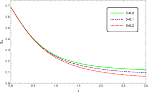
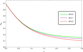
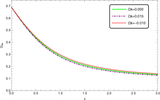
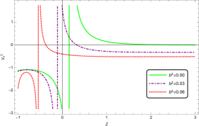
We plot the evolution of and with respect to redshift for BHDE with GO IR cutoff in Fig.1 for different values of Barrow exponent . From this figure, we observe that for , the value of decreases with the increase of while for there is no dependency to . Also the difference between in standard cosmology () and modified Barrow cosmology has been larger in the past. It should be noted that the parameters and are in the range of and [52], respectively, and we find that the best agreement for our model achieves for and . Thus in the rest of this paper we will use these values of and .
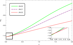
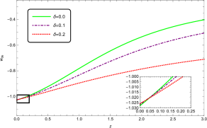
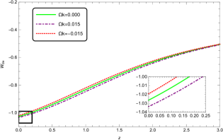
Let us probe in more detail the EoS parameter in Fig.1. A overall harvest is that by increasing the Barrow exponent , the EoS parameter decreases. According to this figure, the EoS parameter at present time crosses the phantom divide . It is worth noting that for , the lies in the phantom regime and for larger , the phantom divide is crossed earlier. One should note that this behavior is cannot be seen in the non-interacting BHDE with future event horizon as IR cutoff [47].
The deceleration parameter is obtained as
| (32) |
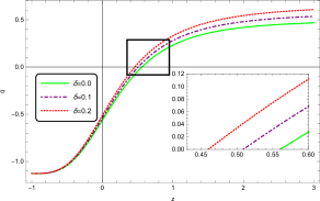
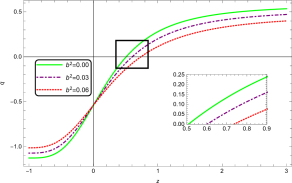
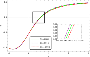
The evolution of the deceleration parameter in terms of the redshift parameter is presented in Fig.2. According to this figure, we find that by increasing the Barrow exponent, , the transition from a decelerated universe to an accelerated universe happens in the lower redshifts. For example for , the phase transition occurs at . Thus increasing parameter leads to a delay in the cosmic phase transition during the history of the universe.
3.3 Interacting case
Next we analyze a FRW universe filled by BHDE and DM, while swapping energy among them. Since the microscopic nature of both DE and DM is still unknown, there exist enough room to leave a chance of interaction between DE and DM [53]. Beside it is shown that in the presence of interaction between two dark components the coincidence problem could be alleviated [54, 55]. In [56], the interaction between DM and DE has been extensively investigated from a thermodynamic point of view. Thus there exist enough motivation and interest to explore an interacting version of dark components. The semi-conservation equations including the interaction between DM and DE read
| (33) |
| (34) |
where is the interaction term, with is a coupling constant and [57]. The negative sign of indicates a transfer of energy from DE to DM. The interaction between dark components affects evolution of the model. Following a same steps as the previous subsection one can find the resulting equations for , as well as the evolution equation of . At first step Substituting and from the conservation equation (33) and (34) into time derivative of modified Friedmann equation (15), we find
| (35) |
In the next step, dividing the modified Friedmann equation in a flat universe (15) by and according to Eq.(35), we arrived the EoS parameter as
| (36) |
Then we obtain evolution equation of the HDE in Barrow cosmology, This equation versus redshift reads
| (37) |
Also, the deceleration parameter can be written as
| (38) |
We found the EoS parameter and the deceleration parameter in this case and equations (28) and (38) are reconstructed. Therefore, the existence of interaction appeared in the evolution of the fractional density parameter against redshift.
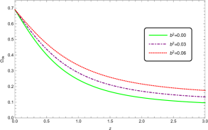
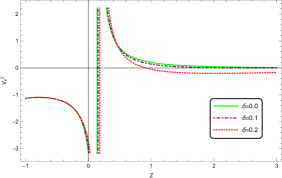
The evolution of versus redshift for different values of and is plotted in Fig.3. Notice that at each , decreases as decreases. From right panel of Fig.3 one can find that Barrow exponent can affects the universe at earlier epochs while its impact at present epoch it has no significant effect.
Next we turn to as well as for a more deep description of the model. At first, one can easily see that and in the interacting HDE of interest reduce to the corresponding relations in the non-interacting case by setting . A close look to left panel of Fig.4 reveals that with increasing the coupling constant , the EoS parameter decreases as well. For all choices of , lies in the phantom regime at the present epoch.
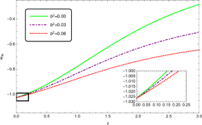
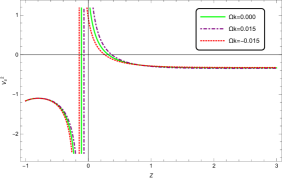
In the left plot of Fig.5, the evolution of the deceleration parameter as a function of redshift is shown for different values of coupling constant . For , the phase transition occurs at while for , the phase transition occurs at . Despite the effects of , increasing causes an earlier phase transitions.

4 HDE in nonflat universe
There exist observational evidences reveal that our observed Universe is not exactly flat and there exist signs of a nonflat geometry [58]-[62]. Thus, it is well motivated to consider dynamics of a nonflat universe. In order to study the dynamics of a nonflat universe filled with BHDE and DM, we introduce the corresponding curvature density parameter, . The first modified Friedmann equation through Barrow entropy in a nonflat universe is
| (39) |
Taking the time derivative of the above equation and using and from the continuity equations Eqs.(34) and (33), we find
| (40) |
As mentioned, is the ratio of DM density to DE density. Dividing Eq.(39) by and substituting Eq.(16), we arrive at
| (41) |
Substituting Eq.(40) and after a little algebra and mixing the related relations, we find
| (42) |
One can easily check that this equation reduce to the corresponding one in the flat background for . Evolution of the fractional energy densities versus redshift according to and Eq.(33) are obtained as
| (43) |
| (44) |
Since the relations are messy analytic description of the model look hard and thus we disclose different features of the model through numerical analysis. On this way we plotted evolution of against redshift in open, flat and close geometry in Fig.6.
Evolution of the EoS parameter for interacting BHDE in Barrow cosmology in non-flat and flat universes are shown in Fig.7. For all choices of the free parameters crosses the phantom regime at present epoch in agreement with observations.
According to obtained term for in non-flat universe Eq.(40), the deceleration parameter is written as
| (45) |
The evolution of the deceleration parameter versus redshift in presence of interaction among dark sector components in non-flat and flat universe are presented in Fig.8. From this figure, we see that for open universe, the transition from deceleration to acceleration happened at lower redshift and for closed universe, the transition from deceleration to acceleration happened at higher redshift also for flat universe, the transition happened at . These indicates that all cases are consistent with observations, [63] depending on suitable choices of the free parameters.
5 Stability and Statefinder of the model
5.1 Stability
Squared sound speed() analysis, is an interesting method which reveals sounds of gravitational instability through a semi-Newtonian approach. In an expanding background, deep inside the horizon, one can find evolution of the cosmic perturbations as
| (46) |
where . The negative and positive signs of could be a sound of instability and stability respectively. To proceed the analysis, we start with definition of the adiabatic squared sound speed which reads
| (47) |
where and are the pressure and the density of the DE component, respectively. According to , Eq.(47) can be written as
| (48) |
Substituting from the conservation equation (33), one may get
| (49) |
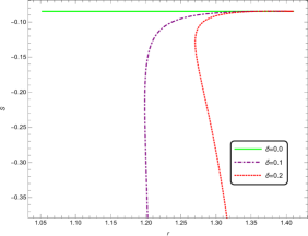
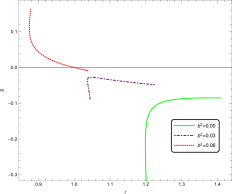
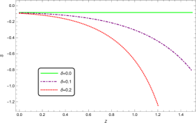
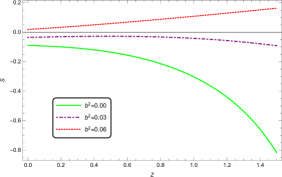
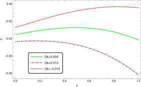
Effects of and the coupling constant are shown in Fig.9. It can be seen that increasing of , the ability in the model decreases. It is interesting that takes positive values in the past and tends to positive values in the future, Fig.9(a). In this model, evidences of instability is seen in the presence of an interaction between DM and DE in the past Fig.9(b). Also, the stability analysis results of the flat, open and closed universe are almost similar. is positive in the near past and near future Fig.9(c).
(a)
 (b)
(b)
 (c)
(c)
5.2 Statefinder
Sahni et al. [64] introduced the statefinder pair , which includes third time derivative of the scale factor . Since DE models are very diverse, it is useful and essential to distinguish between different DE models. The statefinder pair is an effective tool for finding differences between DE models and the standard model(CDM). It should be noted, for the standard model CDM the statefinder parameters are . The statefinder pair is defined as [64],[65]
| (50) |
| (51) |
Based on the relationship between and the deceleration parameter , the parameter could be obtained as
| (52) |
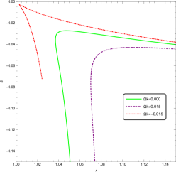
We plotted the evolution of as a function of for different value of , and also for closed, open and flat universe in Fig.10 and Fig.11. As expected, increasing , the BHDE in Barrow cosmology model becomes more different with respect to CDM, which is evident in Fig.10(a) and Fig.11(a). Also, by increasing , the statefinder parameters tend to the values and and in a special case for , the statefinder parameters catch the values at the present time. This means that the our interested HDE in Barrow cosmology model is close to the at the present time in the interacting case according to Fig.10(b) and Fig.11(b). In an open universe the model evolves close to the values and in the past epochs which can be seen in Fig.10(c) and Fig.10(c).
(a)
 (b)
(b)
 (c)
(c)
(a)
 (b)
(b)
 (c)
(c)
6 Conclusions
Based on thermodynamics-gravity conjecture and holographic principle, on the cosmological setups, any modification to the entropy, not only change the energy density of the HDE but also leads to the modified Friedmann equations. In most studies on HDE through modified entropy expression, people consider a modified expression for the HDE density, while they still use the usual Friedmann equations in standard cosmology. This is not compatible with thermodynamics-gravity conjecture, which implies that using the first law of thermodynamics and modified entropy expression, the cosmological field equations get modified as well.
In this work we have investigated BHDE model with GO cutoff in the background of modified Barrow cosmology. We have examined several cases, including DE dominated universe, a flat universe filled with BHDE and DM which evolves separately, a flat universe filled with interacting BHDE and DM. We find that, regardless of the interaction term between two dark components, the EoS parameter, , decreases by increasing the Barrow exponent during the history of the universe, and crosses the phantom divide at the present time. Also the Barrow exponent changes the time of the universe phase transition. We observed that increasing parameter leads to a delay in the cosmic phase transition during the history of the universe. In other words, the phase transition of the universe take place at lower redshift by increasing . Also for a fixed value of Barrow exponent , by increasing the interaction parameter , the value of EoS parameter decreases in all epochs.
We also generalized our studies to a nonflat universe. We found that in flat and non-flat universe, the EoS parameter crosses the phantom regime and we saw that all cases are compatible with observations, [63] depending on suitable choices of the free parameters.
We also explored the sound stability and statefinder of this model and found out that by increasing of , the stability of the model decreases and this model becomes more different with respect to CDM.
Acknowledgements:The work of A. Sheykhi is based upon research funded by Iran National Science Foundation (INSF) under project No. 4024978.
Competing interests: The authors declare there are no competing interests.
Availability of data:This manuscript does not report data.
References
- [1] A. G. Riess et al, Observational evidence from supernovae for an accelerating universe and a cosmological constant, Astron. J. 116, 1009 (1998).
- [2] S. Perlmutter et al, Measurements of omega and lambda from 42 high-redshift supernovae, Astron. J. 517, 556 (1999).
- [3] E. Lusso, E. Piedipalumbo, G. Risaliti, M. Paolillo, S. Bisogni, E. M. A. N. U. E. L. E. Nardini, L. O. R. E. N. Z. O. Amati, Tension with the flat CDM model from a high-redshift Hubble diagram of supernovae, quasars, and gamma-ray bursts, Astron. Astrophys. 628, L4(2019).
- [4] Di Valentino E., et al., 2021, Astropart. Phys., 131, 102605.
- [5] Riess A. G., Casertano S., Yuan W., Macri L. M., Scolnic D., 2019, The Astrophysical Journal, 876, 85.
- [6] Riess A. G., Casertano S.,YuanW., Bowers J. B., Macri L., Zinn J. C., Scolnic D., 2021, Astrophys. J. Lett., 908, L6.
- [7] R. Bousso, A covariant entropy conjecture, J. High Energy Phys. 1999, 004 (1999).
- [8] G. ’t Hooft, Dimensional Reduction in Quantum Gravity, arXiv:gr-qc/9310026.
- [9] L. Susskind, The world as a hologram, J. Math. Phys. 36, 6377 (1995).
- [10] A. G. Cohen, D. B. Kaplan, A. E. Nelson Effective field theory, black holes, and the cosmological constant, Phys. Rev. Lett. 82, 4971 (1999).
- [11] S. Wang, Y. Wang, M. Li, Holographic dark energy, Phys. Rep. 696, 1 (2017).
- [12] S. D. Hsu, Entropy bounds and dark energy, Phys. Lett. B 594, 13 (2004).
- [13] M. Li, A model of holographic dark energy, Phys. Lett. B 603, 1 (2004).
- [14] S. Wang, Y. Wang, M. Li, Holographic dark energy, Phys. Rep. 696, 1 (2017).
- [15] L. N. Granda, A. Oliveros, Infrared cut-off proposal for the holographic density, Phys. Lett. B 669, 275 (2008).
- [16] L. N. Granda, A. Oliveros, New infrared cut-off for the holographic scalar fields models of dark energy, Phys. Lett. B 671, 199 (2009).
- [17] J. D. Barrow, The area of a rough black hole, Phys. Lett. B 808, 135643 (2020).
- [18] E. N. Saridakis, Barrow holographic dark energy, Phys. Rev. D 102, 123525 (2020).
- [19] T. Jacobson, Thermodynamics of spacetime: the Einstein equation of state, Phys. Rev. Lett. 75, 1260 (1995).
- [20] T. Padmanabhan, Gravity and the thermodynamics of horizons, Phys. Rep. 406, 49 (2005).
- [21] T. Padmanabhan,Thermodynamical aspects of gravity: new insights, Rep. Prog. Phys. 73, 046901 (2010).
- [22] A. Paranjape, S. Sarkar, T. Padmanabhan, Thermodynamic route to Field equations in Lanczos-Lovelock Gravity, Phys. Rev. D 74, 104015 (2006).
- [23] A. V. Frolov, L. Kofman, Inflation and de Sitter thermodynamics, J. Cosmol. Astropart. Phys. 2003, 009 (2003).
- [24] B. Wang, E. Abdalla, R. K. Su, Relating Friedmann equation to Cardy formula in universes with cosmological constant, Phys. Lett. B 503, 394 (2001).
- [25] R. G. Cai and S. P. Kim, First Law of Thermodynamics and Friedmann Equations of Friedmann-Robertson-Walker Universe, JHEP 0502, 050 (2005).
- [26] E. Verlinde, On the Origin of Gravity and the Laws of Newton, J. High Energy Phys. 1104, 029 (2011).
- [27] R. G. Cai, L. M. Cao, N. Ohta, Friedmann equations from entropic force, Phys. Rev. D 81, 061501 (2010).
- [28] N. Cai, L. M. Cao, Y. P. Hu, Corrected entropy-area relation and modified Friedmann equations,J. High Energy Phys. 2008, 090 (2008).
- [29] A. Sheykhi, Entropic corrections to Friedmann equations, Phys. Rev. D 81, 104011 (2010).
- [30] A. Sheykhi, Thermodynamics of apparent horizon and modified Friedmann equations, Eur. Phys. J. C 69, 265 (2010).
- [31] A. Sheykhi, S. H. Hendi, Power-law entropic corrections to Newton’s law and Friedmann equations, Phys. Rev. D 84, 044023 (2011).
- [32] S. I. Nojiri, S. D. Odintsov, E. N. Saridakis,Modified cosmology from extended entropy with varying exponent,Eur. Phys. J. C 79, 242 (2019).
- [33] E. M. Abreu, J. A. Neto, E. M. Barboza Jr, A. C. Mendes, B. B. Soares, On the equipartition theorem and black holes non-Gaussian entropies, Mod. Phys. Lett. A 35, 2050266 (2020).
- [34] R. G., Cai, S. P. Kim, First law of thermodynamics and Friedmann equations of Friedmann-Robertson-Walker universe, J. High Energy Phys. 2005, 050 (2005).
- [35] M., Akbar, R. G. Cai, Thermodynamic behavior of the Friedmann equation at the apparent horizon of the FRW universe, Phys. Rev. D 75, 084003 (2007).
- [36] A. Sheykhi, B. Wang, R.G. Cai, Thermodynamical Properties of Apparent Horizon in Warped DGP Braneworld, Nucl. Instrum. Methods Phys. Res. 779, 1 (2007).
- [37] A. Sheykhi, B. Wang, R. G. Cai, Deep connection between thermodynamics and gravity in Gauss-Bonnet braneworlds, Phys. Rev. D 76, 023515 (2007).
- [38] E. N. Saridakis, Modified cosmology through spacetime thermodynamics and Barrow horizon entropy, J. Cosmol. Astropart. Phys. 07, 031 (2020).
- [39] A. Sheykhi, Barrow entropy corrections to Friedmann equations, Phys. Rev. D 103, 123503 (2021).
- [40] A. Sheykhi, Modified cosmology through Barrow entropy, Phys. Rev. D 107, 023505 (2023).
- [41] E. N. Saridakis, Barrow holographic dark energy, Phys. Rev. D 102, 123525 (2020).
- [42] S. Srivastava, U. K. Sharma, Barrow holographic dark energy with Hubble horizon as IR cutoff, Int. J. Geom. Meth. Mod. Phys. 18, 2150014 (2021).
- [43] P. Adhikary, S. Das, S. Basilakos, E. N. Saridakis, Barrow holographic dark energy in a nonflat universe, Phys. Rev. D 104, 123519 (2021).
- [44] F. K. Anagnostopoulos, S. Basilakos, E. N. Saridakis, Observational constraints on Barrow holographic dark energy, Eur. Phys. J. C 80, 826 (2020).
- [45] M. P. Dabrowski, V. Salzano, Geometrical observational bounds on a fractal horizon holographic dark energy, Phys. Rev. D 102, 064047 (2020).
- [46] A. Oliveros, M. A. Sabogal, M. A. Acero, Barrow holographic dark energy with Granda-Oliveros cutoff, Eur. Phys. J. Plus 137, 783 (2022).
- [47] A. Sheykhi, M. Sahebi Hamedan, Holographic Dark Energy in Modified Barrow Cosmology, Entropy 25, 569 (2023).
- [48] A. Sheykhi, S. Ghaffari, Note on agegraphic dark energy inspired by modified Barrow entropy, Physics of the Dark Universe 41, 101241 (2023).
- [49] A. Sheykhi, B. Farsi, Growth of perturbations in Tsallis and Barrow cosmology, Eur. Phys. J. C 82, 1111 (2022).
- [50] A. Sheykhi, Friedmann equations from emergence of cosmic space, Phys. Rev. D 87, 061501(R) (2013).
- [51] S. A. Hayward, Unified first law of black hole dynamics and relativistic thermodynamics, Class. Quant. Grav. 15, 3147 (1998).
- [52] M. T. Manoharan, Eur. Phys. J. C 84, no.5, 552 (2024) doi:10.1140/epjc/s10052-024-12926-z
- [53] C. Wetterich, Nucl. Phys B. 302, 668 (1988).
- [54] Bertolami O, Gil Pedro F and Le Delliou M 2007 Phys. Lett. B 654 165.
- [55] G. Olivares, F. Atrio, D. Pavon, Phys. Rev. D 71 (2005) 063523.
- [56] S. H. Pereira, J. F. Jesus, Can dark matter decay in dark energy?, Phys. Rev. D 79, 043517 (2009).
- [57] D. Pavon, W. Zimdahl, Holographic dark energy and cosmic coincidence, Phys. Lett. B 628, 206 (2005).
- [58] C. L. Bennett, M. Bay, M. Halpern, G. Hinshaw, C. Jackson, N. Jarosik, E. L. Wright, The microwave anisotropy probe* mission, Astrophys. J. 583, 1 (2003).
- [59] D. N. Spergel, L. Verde, H. V. Peiris, E. Komatsu, M. R. Nolta, C. L. Bennett, E. L. Wright, First-year Wilkinson Microwave Anisotropy Probe (WMAP)* observations: determination of cosmological parameters, Astrophys. J. 148, 175 (2003).
- [60] M. Tegmark, M. A. Strauss, M. R., Blanton, K. Abazajian, S. Dodelson, H. Sandvik, D. G. York, Cosmological parameters from SDSS and WMAP, Phys. Rev. D 69, 103501 (2004).
- [61] U. Seljak, A. Slosar, P. McDonald, Cosmological parameters from combining the Lyman- forest with CMB, galaxy clustering and SN constraints, J. Cosmol. Astropart. Phys. 2006, 014 (2006).
- [62] D. N. Spergel, R. Bean, O. Doré, M. R. Nolta, C. L. Bennett, J. Dunkley, E. L. Wright, Three-year Wilkinson Microwave Anisotropy Probe (WMAP) observations: implications for cosmology, Astrophys. J. 170, 377 (2007).
- [63] E. Komatsu, et al., Seven-Year Wilkinson Microwave Anisotropy Probe (WMAP) Observations: Cosmological Interpretation, Astrophys. J. Suppl. 192 (2011) 18. arXiv:1001.4538, doi:10.1088/0067- 0049/192/2/18.
- [64] V. Sahni, T. D. Saini, A. A. Starobinsky, U. Alam, Statefinder—a new geometrical diagnostic of dark energy, J. Exp. Theor. Phys. 77, 201 (2003).
- [65] U. Alam, V. Sahni, T. Deep Saini, A. A. Starobinsky, Exploring the expanding universe and dark energy using the Statefinder diagnostic, Mon. Not. R. Astron. Soc 344, 1057 (2003).