Graded lithium-ion battery pouch cells to homogenise current distributions and mitigate lithium plating
Abstract
Spatial distributions in current, temperature, state-of-charge and degradation across the plane of large format lithium-ion battery pouch cells can significantly impact their performance, especially at high C-rates. In this paper, a method to smooth out these spatial distributions by grading the electrode microstructure in-the-plane is proposed. A mathematical model of a large format pouch cell is developed and validated against both temperature and voltage experimental data. An analytic solution for the optimal graded electrode that achieves a uniform current distribution across the pouch cell is then derived. The model predicts that the graded electrodes could significantly reduce the likelihood of lithium plating in large format pouch cells, with grading increasing the C-rate at which plating occurs from 2.75C to 5.5C. These results indicate the potential of designing spatially varying electrode architectures to homogenise the response of large format pouch cells and improve their high rate performance.
1 Introduction
Lithium-ion battery electrodes are complex non-linear dynamical systems reacting non-uniformly in space and time, especially when subject to high C-rate currents. Phenomena such as travelling wave fronts in charging LiFePO4 (LFP) cathodes 1; 2 and localised lithium-plating in graphite anodes 3 are just some examples of the diverse range of non-linear behaviours that have been observed in battery electrodes, and it is these localised behaviours that often govern cell performance. To protect against these spatially localised electrochemical behaviours, the use of graded electrode structures (as in those with controlled spatial variations in electrode microstructure) has been proposed with the idea being that introducing heterogeneity into the electrode microstructure can reduce the heterogeneity in the electrochemical response.
Recently, experimental data have provided support for the use of graded electrodes in practical cells 4. A common theme is the potential of graded electrodes to increase both the capacity at high C-rates 5; 6 and the cycle life of thick electrodes 7; 8, with other benefits including a reduction in electrode tortuosity 9. Data for both standard electrodes, such as LFP cathodes 7; 8, and non-standard electrodes, such as anodes arranged in a layered structure composed of high power Li4Ti5O12 and high capacity SnO2 10, have shown similar benefits. However, care has to be taken when designing graded electrodes, as structuring the electrode incorrectly can deteriorate performance 11; 8. To prevent this, mathematical models have been developed to predict the electrochemical response of graded electrodes so as to quickly and cost-effectively optimise their designs. Several different models have now been developed covering a range of length scales (including micro-structural12; 13 and Doyle-Fuller-Newman-type models14; 2) and performance metrics (such as fast charging capacitance 2 and electrical impedance 15). These results highlight the growing maturity of battery modelling and parameterisation, which, in turn, is making it increasingly straightforward to embed modelling pro-actively in the battery design process 16. An example of this battery co-design process are the trapezoidal electrodes7 that were developed using insights 15 on how the distribution of carbon and binder affects the conductivity of the LiFePO4 electrodes.
The focus of most existing studies on graded electrodes for lithium-ion batteries has been on controlling the through-thickness local electrode microstructure 12; 17, including bilayer cathodes2 composed of discrete layers of both Li[Ni0.6Co0.2Mn0.2]O2 (NMC622) and LFP. Focusing on the through-thickness electrode structure (with experiments typically only involving coin cells 7) is justified by the fact that it is charge mobility through the electrode thickness between the anode and cathode that governs coin cell performance. However, in recent years, there has been a general trend in commercial cells towards larger cell formats (demonstrated, for example, by the introduction of the larger 4680 cylindrical cells 18). The idea being that larger cell formats increase the specific energy density, as the ratio of active material to superfluous materials such as casings and control circuits is increased. Large format cells have their own problems compared to coin cells; in particular, they experience new forms of spatial heterogeneities, which emerge at the macro-scale (as in across their width and length). In particular, thermal hot spots 19; 20 and spatially localised distributions of electrode degradation 21; 22; 23, lithium plating 24, state-of-charge 25, and currents in-the-plane of large-format pouch cells 26; 27 have been identified as impacting performance, especially in high rate applications.
The significance of in-the-plane spatial heterogeneities on the performance of large format pouch cells is becoming increasingly apparent. In turn, this has driven efforts to understand how these heterogeneities develop using mathematical models. Through these models, predictions for chemical reaction 28 and current distributions along the plane of the current collectors 29 (and how these distributions evolve with changes in the cell’s design, e.g. its current collector thickness 30 and tapering 31) have been developed, with analytical solutions even being proposed 32. The push to understand the planar dynamics of pouch cells has meant that the number of spatial dimensions in these models has increased, with 2D 33 and 3D 34; 35; 36; 37; 20; 38 effects often included, as opposed to the through-thickness models of, for example, the DFN model and single particle models 39; 40. One of the main drawbacks of large format battery models is their complexity, a consequence of their multi-dimensional spatial domains. This model complexity leads to several challenges including long simulation times and difficulties in model parameterisation, as discussed in the electro-thermal modelling studies 1920. These challenges demonstrate a need for easily parameterised and computationally efficient pouch cell models able to capture the spatial distributions seen in experimental data. This problem is considered with the model introduced in Section 2.
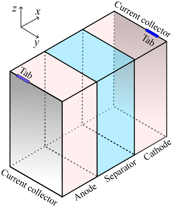
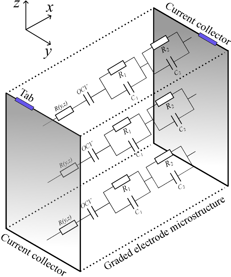
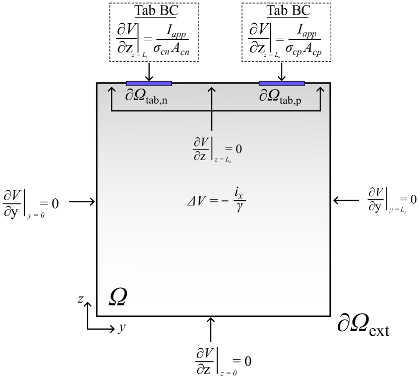
The formation of spatial heterogeneities across pouch cells indicates that it may be possible to grade the local electrode microstructure in-the-plane to mitigate their effect, similar to what has been achieved with through-thickness grading 41; 17. This graded electrode problem is illustrated in Figure 1, with Figure 1(a) indicating the planar and through-thickness directions of the pouch cell, Figure 1(b) indicates the simplification that allows the model to be reduced to a 2D problem, and Figure 1(c) indicates the 2D model domain.
Contributions:
In this paper, the problem of modelling and optimising graded electrode microstructures for large format pouch cells with controlled variations in resistance in-the-plane is considered. The following contributions are obtained:
-
1.
A model for a large format pouch cells is described and validated against experimental data20.
-
2.
An analytic solution for the distribution of carbon black in the electrode plane that achieves a flat current distribution across the pouch cell is derived.
-
3.
Compared to uniform electrodes, it is predicted that graded electrodes can increase the charging rate when lithium plating occurs from 2.75C to 5.2C.
It is proposed that a primary advantage of these graded pouch cells is to mitigate the impact of lithium plating (see Section 4), as the flatter current distributions reduce the likelihood of negative anode overpotentials. The results highlight the importance of in-the-plane effects when characterising lithium plating in large format cells. By contrast, it is shown that the high thermal/electronic conductivity of the current collectors means that only minimal benefits of grading are observed when considering the thermal and voltage response; Section 3.4 shows that the graded cells only delivered a 1.2% increase in stored capacitance for 4C charging compared to the uniform electrodes, a conclusion in agreement with Hosseinzadeh, et al. 201841. These validated modelling results indicate the potential of grading to improve the cycle-life and high-rate performance of large format pouch cells. More broadly, they indicate how improvements in battery design and manufacturing could reduce the performance gap observed between coin cells constructed in laboratories and the large format cells used in commercial high-rate applications 42.
2 Mathematical model
In this section, a mathematical model of a large format pouch cell is introduced. Specific focus is given to a comparison between the model and experimental data20, with the presented model being simpler in form (specifically, here, circuit dynamics are used to capture the through-thickness electrical response, whereas a simple electrochemical model is used in Lin, et al, 202220) whilst still being able to accurately capture the in-plane spatial distributions seen in the experimental data (see Section 2.5). Keeping the model formulation relatively simple while retaining the important physics-based mechanisms allows analytic solutions to the optimal graded electrode design problem (explored in Section 3) to be obtained, which is the focus of this work.
2.1 Model formulation
Figure 1 presents a schematic for the model’s formulation and spatial domain. The model parameters and variables are defined in Tables A1 and A2. The following assumptions are made:
-
A1:
The current collectors’ thicknesses are much thinner than their width and height.
-
A2:
The circuit models of Figure 1(b) describe the electrical dynamics at each point in the plane of the pouch cell.
- A3:
A1 is justified because large format pouch cells are considered (with typical current collector thicknesses being m and their planar dimensions being 15cm 20cm). Defining as the charging current through the electrode, and as the current flowing in the -direction through current collector , then, under this thin plate assumption, the current gradient in the -direction through the current collectors can be approximated by
| (1) |
following the ideas of Taheri, et al. 201432. A2 is a simplification of the electrodes’ electrical dynamics, but, even so, the resulting model is able to capture the spatial distributions seen in the experimental data (see Section 2.5) while being simple enough to generate an analytic solution to the optimal electrode design problem (Section 3.1) and parameterise (illustrated by the relative lack of parameters in Table A2). A3 is justified under the assumption that each layer has a similar composition and so react similarly.
2.2 Model equations
The following equations characterise the proposed mathematical model for large-format pouch cells, with the models domain described in Figure 1(c). Regarding the notation, each model variable in Eqn. (3) is defined in the ()-plane of the pouch cell, as illustrated in Figure 1(c), and may also evolve in time . This dependency of the variables is dropped in the model equations (3) to ease readability. is the voltage (defined as the potential of the current collector at the cathode minus that of the anode) at each point in the plane, is the cell temperature, is the local through-thickness current, is the local resistance of the two electrodes and the separator that is constant with time, while SoC is the local state of charge in the plane. Table A1 summarises the model’s variables, while Table A2 gives its parameters. For the graded cell, the only parameter varying in is , with the rest being constants. Using the notation and defining
| (2) |
then
| (3a) | ||||
| (3b) | ||||
| (3c) | ||||
| (3d) | ||||
| (3e) | ||||
| (3f) | ||||
where is the projection of the cell onto the -plane and and are the cell width and height, respectively. Eqn. (3a) defines the through-thickness current (as in the current flowing across the electrodes charging the active material particles). Eqn. (3b) defines the distribution of the voltage across the two current collectors. Eqn. (3c) defines the localised temperature dynamics of the cell. Using the circuit model of Figure 1(b) to describe the electrical dynamics at each point ( in the plane, Eqn. (3d) describes the state-of-charge and Eqns. (3e)-(3f) are the relaxation dynamics associated with Figure 1(b)’s RC pairs.
2.3 Boundary Conditions
Using the notation of as the two-dimensional unitary vector normal to the boundary and , then the model’s boundary conditions are:
| (4a) | ||||
| (4b) | ||||
| (4c) | ||||
| (4d) | ||||
where and are the negative and positive tabs, , is the external boundary region and is the external boundary region without the tabs, .
2.4 Numerical Solution Procedure
To simulate the model, the partial-differential-algebraic equations of Eqns. (3) and (4) were discretised in space using Chebyshev spectral collocation43 and solved using “ode15s” in MATLAB® 2022b44. On average, a 5C charge of a uniform cell took 12.7 s (with 24x24 nodes) when run on a desktop Macintosh (MacBook Pro, Monterey, v 12.4, M1 2020, 16GB, 256GB, 64 bit). The unknown model parameters were found by fitting to 4C square-wave-excitation experiments starting at 30% SOC 20. The open-source code for the pouch cell model simulations can be found at: https://github.com/EloiseTredenick/2DBatteryTemperatureGradedModel.
Comparison to existing models:
The main differences between the large-format pouch cell model of (3) and existing models 20 32 are: i) the inclusion of the spatially-varying resistance, , in (3), ii) the model’s relative simplicity, with no DFN-type through thickness electrochemical modelling being used; instead, the circuit of Figure 1(b) is distributed in the plane. The relative simplicity of the model is a deliberate design choice as it significantly simplifies the model parameterisation problem, which is crucial for capturing the experimental data.
It is also noted that graded planar cells were also investigated in Hosseinzadeh, et al. 201841, where a DFN-type model with grading both in-the-plane and through-the-thickness of the electrodes was developed. The two main differences between this paper and Hosseinzadeh, et al. 201841 are: i) an analytic solution for planar graded electrodes to achieve a uniform current distribution is obtained here (see Eqn. (7)), ii) this paper’s model predictions are validated against experimental data from Lin, et al, 202220, iii) it is proposed that the benefits of in-the-plane grading are to reduce electrode degradation (especially plating), whereas voltage and thermal considerations were considered in 41.
2.5 Comparison to experimental data
The experimental data from Lin, et al, 202220 is used to validate the lithium-ion battery pouch cell model of (3). Briefly, the data is obtained from square-wave-excitation cycling experiments starting at 30% state of charge (SoC), using 20 Ah pouch cells from A123 Systems with LFP positive electrodes and graphite negative electrodes, which were cycled at 4C (at currents A) every 100 seconds. A thermal imaging camera was then used to capture thermograms of the cell surface and to visualise the cell’s temperature distribution across the plane during the cycling.
2.6 Model validation
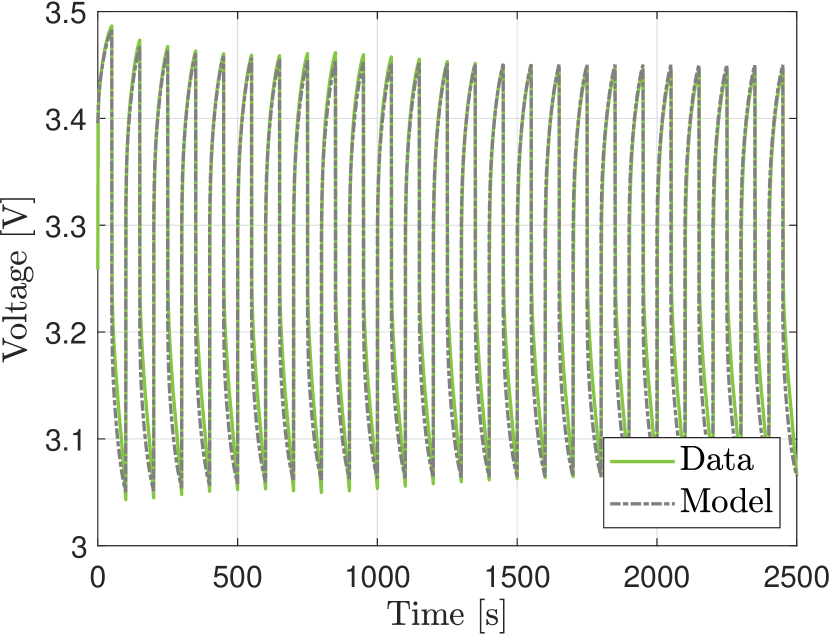
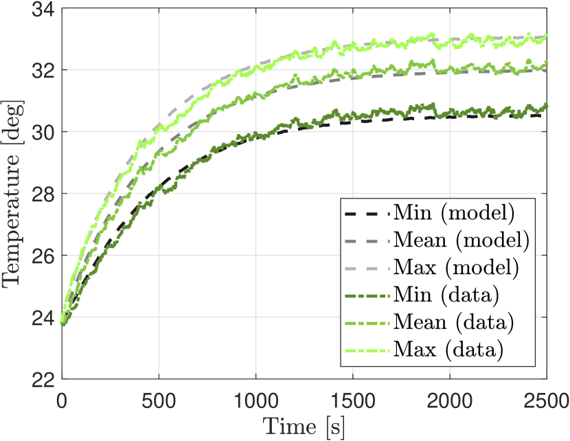
Figures 2 and 3 compares the model simulations against the experimental data20 for cycling using the parameters from Table A2. The parameters were estimated using a combination of fitting and a comparison to values from the literature, with the notation for the resistance of the uniform cell. Model agreement was observed in both the electrical and thermal response, as shown in Figures 2(a) and 2(b).
Figure 2(b) shows that the model was able to capture the evolution of the maximum, minimum, and average values of the cell temperature across the plane of the pouch cell during the cycling. A main point of difference between the trajectories of the model and the experimental data is that the model’s trajectories are much smoother. The increased stochasticity of the data is to be expected, as the sensing noise and the inherent randomness in the microstructure introduced by manufacturing limitations are not captured by Eqn. (3). However, the model is still able to capture the general trends of the data, with the time constants and steady-state values of the first-order responses seen in the temperature dynamics being captured.
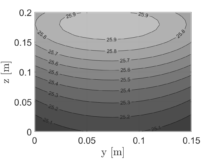
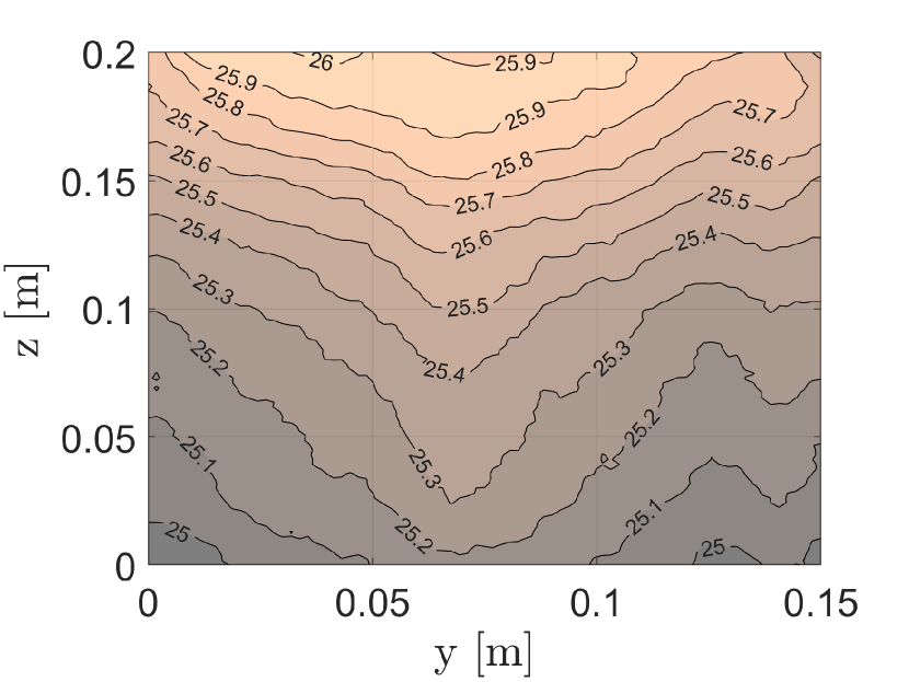
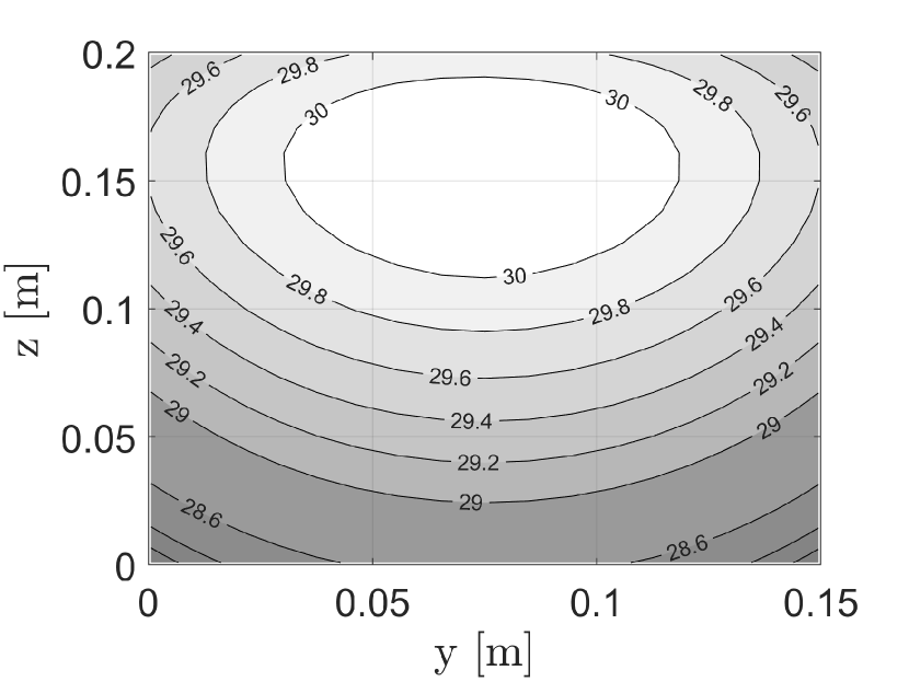
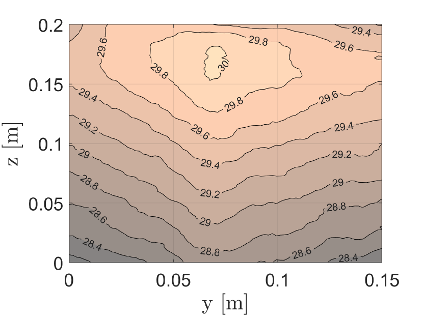
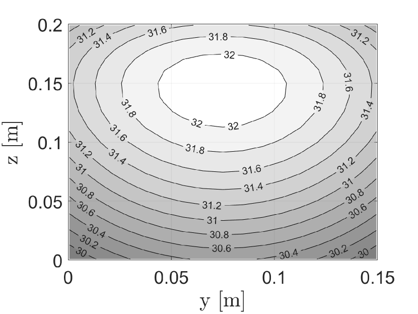
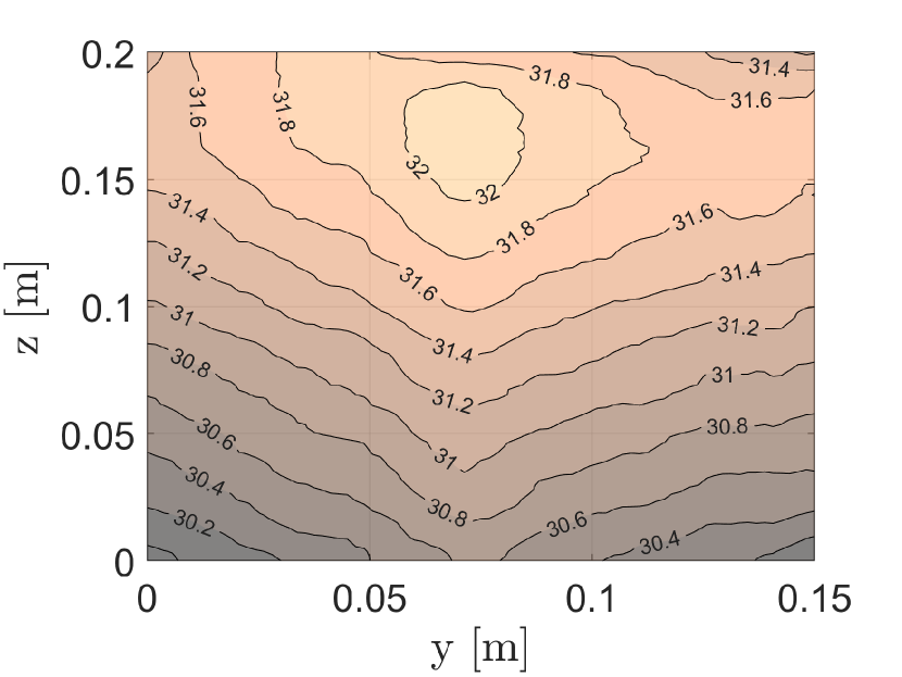
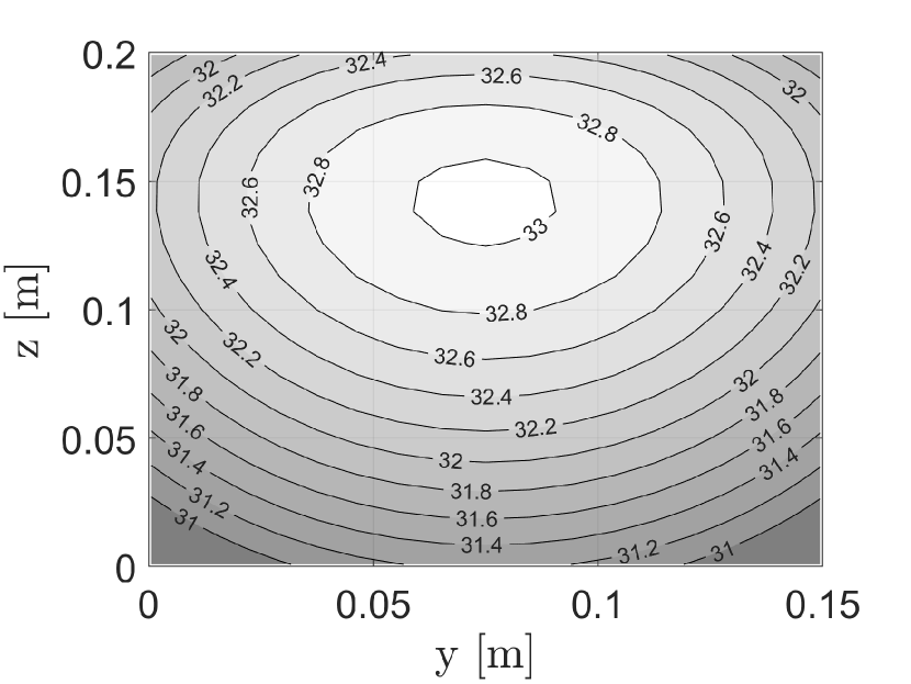
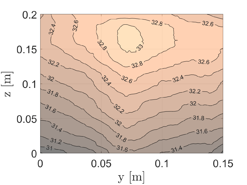
Figure 3 compares snapshots in the plane of the temperature distribution of the model and the experimental data 20, where the snapshots were taken at 100s, 500s, 1000s, and 2500s. Even though the underlying model of Eqn. (3) is simple, strong agreement was made with the experimental thermal data from Lin, et al, 202220. In particular, the formation of a thermal hot spot as well as the general shape of the temperature contours were captured by the model, although, again, the model’s diffusion dynamics resulted in smoother contours than those seen in the data.
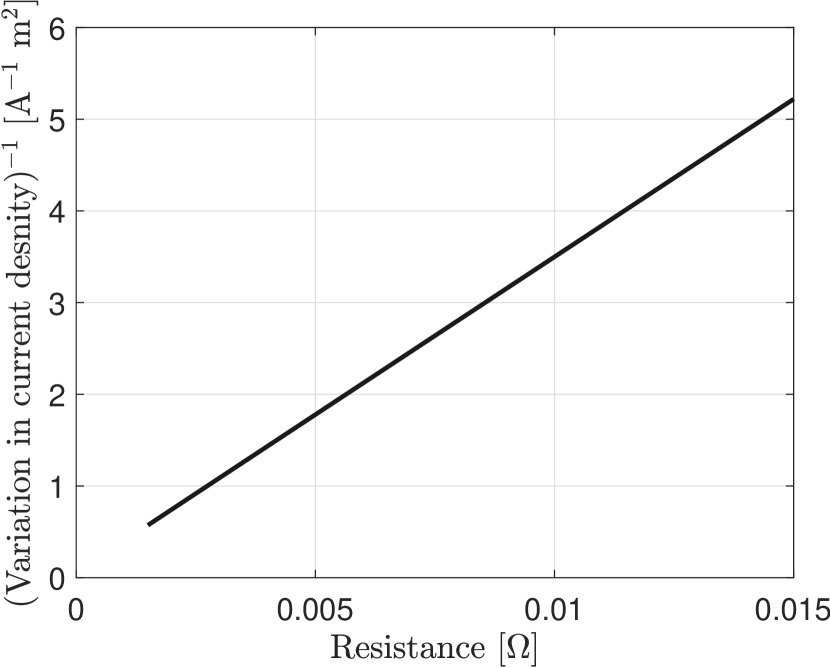
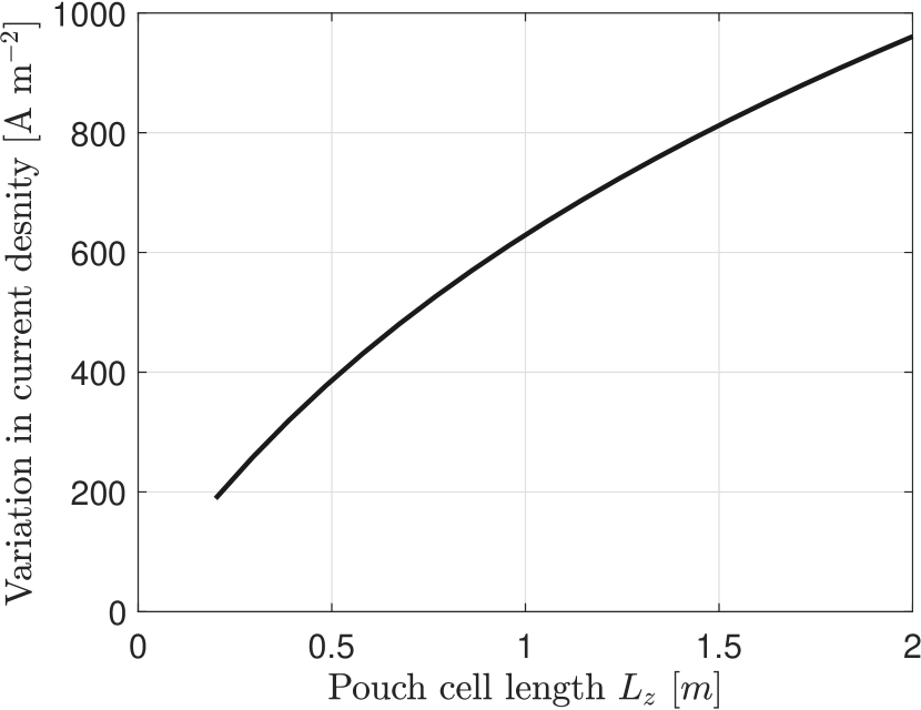
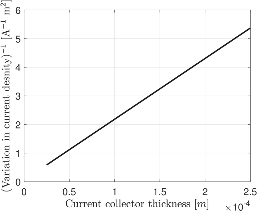
Figure 4 illustrates how the validated model could be used to infer the impact of design changes in the pouch cell on the degree of spatial heterogeneity across the plane. Defining the variation in the current density as the difference between the maximum and minimum current density across the plane, Figure 4(a) shows how this variation changes with resistance (as in, with ), Figure 4(b) shows how it changes with pouch cell length, and Figure 4(c) shows how it changes with current collector thickness. The figure identifies some near linear relationships between these cell parameters and the variation in current density, with explicit characterisations for these expressions obtainable from the analytical solution of Taheri, et al, 201432. As could be expected, the figure indicates that the variation of the current distribution across the pouch cell increases as: i) the cell resistance decreases, ii) the aspect ratio increases, and iii) the current collectors get thinner. Notably, Figure 4(a) indicates that as the cell ages, and so as its resistance increases, the variation in current distribution across the cell is likely to decrease, as more current is encouraged to flow along the current collectors than through the thickness of the cell.
3 In-the-plane electrode grading
The spatial distributions seen in the response of the pouch cell, for example in the temperature data of Figure 3, presents an opportunity to apply electrode grading to create a more uniform electrochemical response. In this section, an analytic solution for the resistance distribution across the plane of the pouch cell, , to achieve a uniform current distribution is described.
3.1 Grading manufacturing
It is assumed that the electrode resistance can be controlled locally in space. The reasons for focusing on the resistance distribution are: i) following Eqns. (3a) and (3b), the electrode resistance directly influences the current distribution across the pouch cell (and it is variations in the current which are targeted to be smoothed out by the optimally graded electrode), ii) existing results on through-thickness electrode grading have demonstrated how this resistance grading can be achieved, e.g. by controlling the relative mass fraction of carbon black in LFP cathodes using spray printing techniques 15. It is envisaged that such spray techniques could be generalised to produce the optimised planar graded electrodes proposed in this study.
3.2 Resistance distribution for homogeneous current
The problem of distributing the resistance (achieved by controlling the weight fraction of active carbon in the electrode microstructure) to achieve homogeneous current distribution across the pouch cell is considered. This targeted flat current distribution is equal to the average current density, with
| (5) |
Eqn. (3) implies that, under isothermal conditions of the open-circuit voltage, if a uniform current distribution is achieved at , then , and the SoC, will evolve uniformly in space as well. The implication is that if the current distribution is uniform at , it will remain uniform during the simulation, following the model equations of (3a) and (3b), which may not hold exactly in practice as local current spikes might emerge caused by the variability in the local electrode composition. However, this can be used to simplify the graded electrode design optimisation problem. Specifically, it converts a dynamic optimisation problem into a static one. As in, it changes the optimisation from one of determining how the resistance should be distributed to achieve a uniform current during the whole charge to one that only has to consider the distribution at the start of the charge. A consequence of this problem formulation is that it allows an analytic solution to the graded electrode design optimisation to be derived (see Eqn (7)).
3.2.1 Problem formulation
With the above motivation, the desired uniform current distribution of Eqn. (5) is substituted into Eqns (3a) and (3b) to give, after simplifying,
| (6a) | ||||
| which is a non-homogeneous Laplace equation in the spatial variable . Using the same approach, the boundary conditions for the voltages from Eqns. (4c) and (4d) can be translated into boundary conditions for the resistance to achieve a uniform current density, as in | ||||
| (6b) | ||||
| (6c) | ||||
3.2.2 Solution
The solution to Eqn. (6) is
| (7a) | ||||
| composed of a quadratic part, , and a hyperbolic part, , satisfying | ||||
| (7b) | ||||
| (7c) | ||||
| The coefficients of this solution are | ||||
| (7d) | ||||
| (7e) | ||||
| (7f) | ||||
| with | ||||
| (7g) | ||||
and the constant being a free variable setting the average value of the resistance.
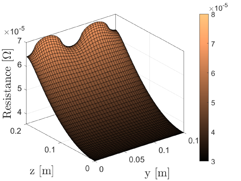
The solution of Eqn (7) shows that the resistance should roughly decrease quadratically away from the tabs in order to flatten the current distribution. The physical meaning of decreasing the resistance away from the tabs is to encourage current to flow down the length of the current collectors, instead of going directly through the electrodes as it enters one of the tabs and leaves the other. In the particular setup of Figure 1 and Table A2, where the cell has a relatively high aspect ratio, the variation of the resistance is much larger in the -direction rather than the -direction, but, following Eqn. (7), this may change for wider cell formats or for different tab configurations.
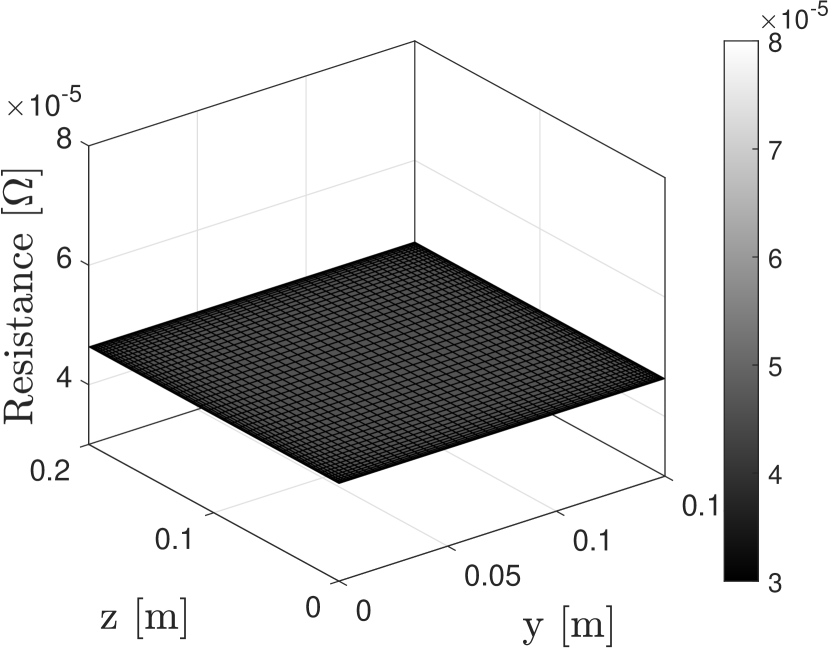
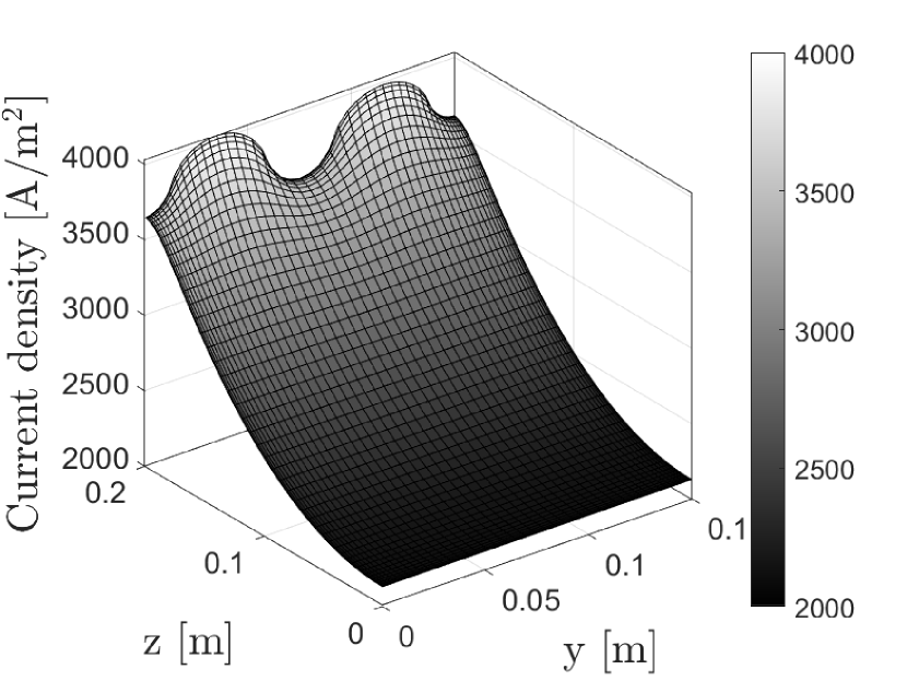
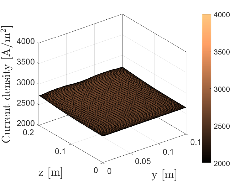
3.3 Results: Flat current distribution across pouch cells
Figure 5 compares the current and resistance distributions achieved with both uniform and graded pouch cells (with the resistance of the graded cells following the solution derived in Eqn. 7). For this analysis, both pouch cells had equal average resistances of 1.5 to ensure a fair comparison. Significant variation was seen in the current density distribution of the uniform cell (with a maximum value of 3925 A m-2 at the tabs and a minimum value of 2138 A m-2 at the opposite end where ). By contrast, the graded cell achieved a constant current density of 2667 A m-2 across the plane, as predicted.
3.4 Results: Dynamic response of graded pouch cells
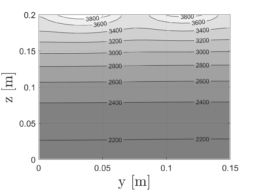
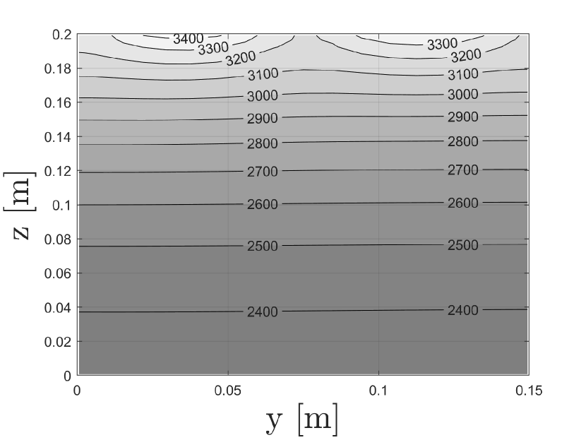
Figure 6 compares the optimised graded electrode cell following Eqn (7) and the uniform cell for a full 4C charge at = 80A. Figure 6 provides justification for the design choice of Section 3.1 to optimise the spatial resistance of the pouch cells to achieve a uniform initial current distribution in space, as Figure 6(a) indicates that this uniformity in the current was retained during the whole charge. By contrast, the current distribution in the uniform cell is more variable. Initially, large current gradients exist across the plane of the uniform cell, as shown in Figure 6(a), with the maximum current density 3925 A/m2 at the tabs and the minimum current 2138 A/m2 at the opposite end. The non-uniform current distribution then causes the voltage to vary, following Eqns. (3d)-(3f). Simultaneously, there is a negative feedback effect acting on the voltages from Eqns. (3a) and (3b) that smoothens this variation. The interactions between these two modes causes the spatial distribution of the current to evolve in both space and time. In particular, Figure 6(a) shows that the current does not change significantly during 100s 450s when the OCV curve is flat (since the smoothing effect of in Eqn. (3a) is not active). It is this smoothing effect which causes the region near the tabs to charge first, but then, when it is fully charged, the majority of the current then flows through the bottom half of the cell.
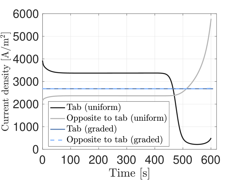
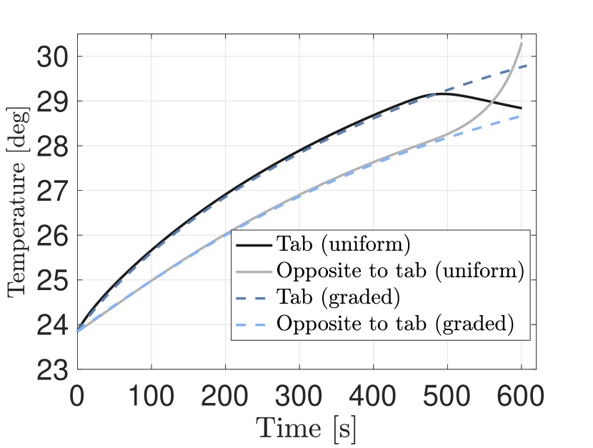
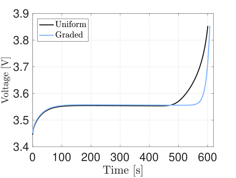
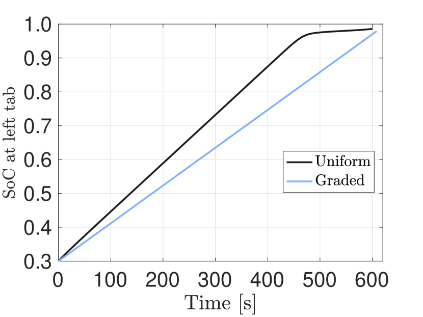
Figure 7 shows snapshots of the current distribution across the current collectors of the pouch cell with uniform electrodes at = 1s, 200s, 500s and 600s during the 4C charge. At the start of the simulation, the peak current was at the tabs, with this peak moving down the cell during the charge. It is noted that the maximum variation in the current distribution in the plane was recorded near the end of the charge, which is also the time when lithium-plating is most likely to occur.
Whilst Figure 6(a) indicates that there would be large differences between the current distributions of the uniform and graded cells, Figures 6(b) and 6(d) indicate that the impact of these differences on the variable internal to the current collectors would actually be quite limited. Specifically, Figure 6(b) compares the temperatures, Figure 6(c) the voltages, and Figure 6(d) the state-of-charges. Although there are some differences between the uniform and graded electrodes, it is relatively limited compared to the large variations seen in the current distributions. In particular, even though the profiles of the two voltage curves in Figure 6(c) are different, they reach the cut-off voltage of 3.85 V at roughly the same time (607s for the graded cell and 600s for the uniform one). As such, the capacitance improvement of the graded cell over the uniform one is only 1.2%. These limited gains in the capacitance are a result of the large thermal and electrical conductivities of the current collectors (see Table A2), which smooth out the variations in the electrodes responses across the plane. Similarly, for the current, Appendix Figure A1 compares the modelled 4C cycling results for the graded and uniform cells. The current density of the graded cell is close to , while the uniform cell has large variations both in time and across the plane. The voltage of both cells is similar, while the maximum temperature is slightly reduced by for the graded cell.
When only variables defined internally to the current collectors (such as temperature and voltage) are used to assess the value of graded pouch cells, their benefits may be lost. This observation agrees with the conclusions of Hosseinzadeh, et al, 201841 that porosity distribution through the electrode thickness has the potential to produce superior battery performance instead of when the porosity is varied along the electrode height. However, in this paper, it is proposed that to unlock the benefits of graded pouch cells, a performance metric that focuses on through-thickness effects should instead be considered. This observation motivates the analysis of the following section on the potential benefits of graded electrodes to mitigate lithium plating.
4 Results: Plating reduction with graded electrodes
The potential of graded electrodes to mitigate lithium plating in large format cells is explored in this section. As discussed in relation to Figures 6(b)-6(d) and in the results of Hosseinzadeh, et al, 201841, it was observed that the high conductivity of the current collectors limits the apparent value of electrode grading in-the-plane when only variables found “internally” to the current collectors (with internal variables being understood as those, such as voltage and temperature, that are smoothed out when flowing in the plane of the current collectors) are used to assess performance, as opposed to variables flowing through the electrodes (such as the current distributions of Figure 7 and 6(a)). However, as lithium plating is a localised degradation phenomenon dependent upon the charging current and electrochemical state of the electrode at a given point, it is shown in this section that plating may be effectively mitigated by in-the-plane electrode grading. The focus towards mitigating lithium plating is also motivated by experimental studies 24 which show significant spatial variations in plating across graphite anodes. Controlling the distribution of active carbon in the electrode microstructure to mitigate the spatial distribution in plating is proposed as a means to reduce the accelerated degradation of large format pouch cells in high-rate applications.
A mathematical modelling approach was used to compare the extent of lithium plating between the graded and uniform cells. However, modelling lithium plating is known to be challenging, with existing models typically being additions to complex electrochemical models, with example models discussed in 45; 46. By contrast, in this paper, a simpler, control-orientated model adapted from 47 was used, with this model based off of the earlier results of 48. For the state-constrained control problem considered in 47, the following condition for lithium plating was developed, with the anode regarded as experiencing plating if the following inequality is satisfied
| (8) |
The plating inequality47 of Eqn. (8) was determined by fitting a curve when the anode over-potential in a DFN model went negative. Here, , , , following 47, and .
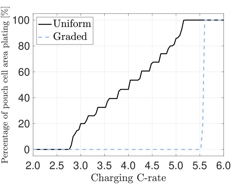
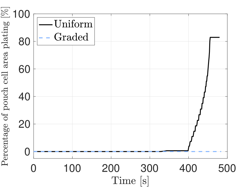
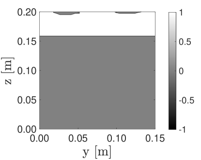
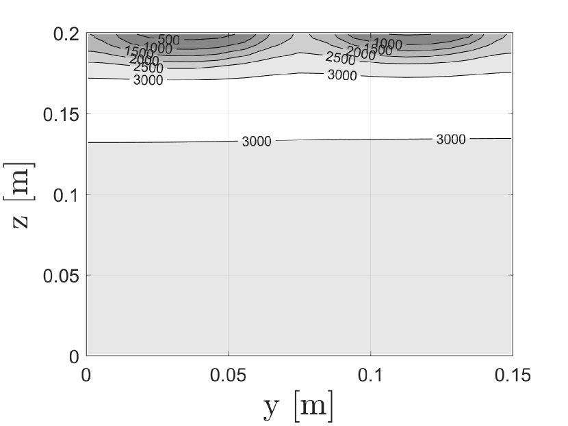
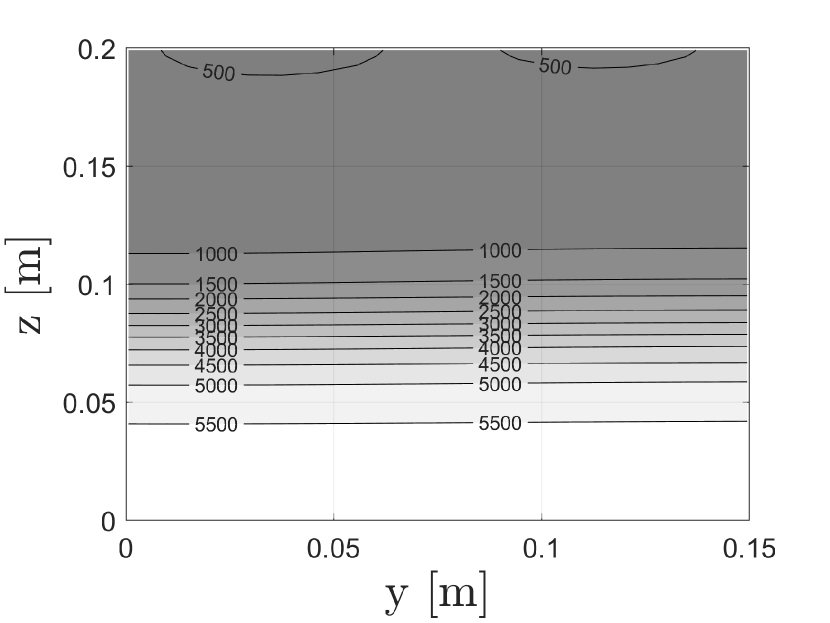
Figure 8 compares the onset of lithium-ion plating for both the uniform and graded pouch cells using Eqn. (8). The purpose of this figure is to illustrate the spatial, temporal and C-rate rate dependence of plating, and how modelling can capture the heterogeneity of pouch cell degradation. Figure 8(a) shows the areal percentage of the pouch cell experiencing plating during charging at different C-rates. The uniform pouch cell sees a gradual increase in the area of the pouch cell experiencing plating when the C-rate is increased beyond 2.75C, with 100% of the pouch cell experiencing plating at 5.2C. By contrast, the graded pouch cell experiences no plating until 5.5C whereupon there is a sudden jump to 100% of its area that is plating. The differences between these two curves is due to variation in the current distribution of the uniform cell; this variation leads to higher current spikes and so a greater likelihood of plating. By contrast, the model predicts that the flatter current distribution of the graded pouch cell can delay the onset of plating until a critical point is reached, and, at that point, the flat distributions cause the whole plane to plate. The significance of this figure is that it suggests that grading pouch cells can increase the maximum charging C-rate for which plating can be avoided. In other words, grading in the plane could increase the operating envelope of pouch cells such that they could be fast charged without suffering from plating.
Figure 8(b) shows the time when plating is initiated during a 5C charge. During this charge, the graded cell does not plate whereas the uniform electrodes experiences plating at the end of charge. The propensity of plating to occur in uniform cells at the end of charge is one of the main reasons why optimal fast charging currents are often tapered at the end of charge49; 50.
Figure 9 illustrates the spatial distribution of plating across the plane of the uniform pouch cell at the end of the 5C charge. The grey area indicates a region where plating is predicted to occur. The figure suggests that, for these cells, most of the plating occurs opposite the tabs with the plating then progressing up the plane. This effect is in response to the current distribution being highest at the tabs at the start of the charge, causing the active particles in this region to be charged first. When these particles become fully charged, they hinder further charging in this region and so cause current to flow down towards the bottom of the pouch cell later on during the charge. By restricting the area where the current can flow through, the local current densities in this region at the bottom of the cell are increased (see also Figure 6(a)), causing a higher likelihood of plating.
Conclusions
A model for large format lithium-ion battery pouch cells with spatial grading across the plane was developed and validated against experimental data. An analytic solution for the optimal electrical resistance distribution across the plane of large format pouch cells to achieve a flat current distribution was derived. The main benefit of graded electrodes identified was to increase the allowable charging C-rate from which lithium plating could be avoided; the graded electrodes increased the safe charging rate from 2.75C to 5.5C. By contrast, only a 1.2% increase in charging capacity was achieved for 4C charging. These results indicate the potential of in-the-plane graded electrode microstructures for enabling fast charging of large format pouch cells that by limiting the spatial heterogeneities.
Acknowledgements
Funding for this work was partially provided by the Faraday Institution project ‘Nextrode - next generation electrodes’ (grant number FIRG015 and FIRG066). RD acknowledges funding by a UKIC Research Fellowship from the Royal Academy of Engineering.
Code Availability
The open-source code for the pouch cell simulations that have been used to produce the results of this study are available online (https://github.com/EloiseTredenick/2DBatteryTemperatureGradedModel).
References
- 1 G. K. Singh, G. Ceder, and M. Z. Bazant, “Intercalation dynamics in rechargeable battery materials: General theory and phase-transformation waves in LiFePO4,” Electrochimica Acta, vol. 53, no. 26, pp. 7599–7613, 2008.
- 2 E. C. Tredenick, S. W. R. Drummond, Y. S. Y, S. R. Duncan, and P. S. Grant, “A multilayer Doyle-Fuller-Newman model to optimise the rate performance of bilayer cathodes in Li ion batteries,” 2024. pre-print.
- 3 A. S. Ho, D. Y. Parkinson, D. P. Finegan, S. E. Trask, A. N. Jansen, W. Tong, and N. P. Balsara, “3d detection of lithiation and lithium plating in graphite anodes during fast charging,” ACS Nano, vol. 15, no. 6, pp. 10480–10487, 2021.
- 4 S. N. Lauro, J. N. Burrow, and C. B. Mullins, “Restructuring the lithium-ion battery: A perspective on electrode architectures,” eScience, p. 100152, 2023.
- 5 E. G. Sukenik, L. Kasaei, and G. G. Amatucci, “Impact of gradient porosity in ultrathick electrodes for lithium batteries,” Journal of Power Sources, vol. 579, p. 233327, 2023.
- 6 R. Chowdhury, A. Banerjee, Y. Zhao, X. Liu, and N. Brandon, “Simulation of bi-layer cathode materials with experimentally validated parameters to improve ion diffusion and discharge capacity,” Sustainable Energy & Fuels, vol. 5, no. 4, pp. 1103–1119, 2021.
- 7 C. Cheng, R. Drummond, S. R. Duncan, and P. S. Grant, “Extending the energy-power balance of Li-ion batteries using graded electrodes with precise spatial control of local composition,” Journal of Power Sources, vol. 542, p. 231758, 2022.
- 8 C. Cheng, R. Drummond, S. R. Duncan, and P. S. Grant, “Combining composition graded positive and negative electrodes for higher performance Li-ion batteries,” Journal of Power Sources, vol. 448, p. 227376, 2020.
- 9 Z. Chen and Y. Zhao, “Tortuosity estimation and microstructure optimization of non-uniform porous heterogeneous electrodes,” Journal of Power Sources, vol. 596, p. 234095, 2024.
- 10 S. H. Lee, C. Huang, and P. S. Grant, “Multi-layered composite electrodes of high power Li4Ti5O12 and high capacity sno2 for smart lithium ion storage,” Energy Storage Materials, vol. 38, pp. 70–79, 2021.
- 11 S. Yari, H. Hamed, J. D’Haen, M. K. Van Bael, F. U. Renner, A. Hardy, and M. Safari, “Constructive versus destructive heterogeneity in porous electrodes of lithium-ion batteries,” ACS Applied Energy Materials, vol. 3, no. 12, pp. 11820–11829, 2020.
- 12 A. M. Boyce, D. J. Cumming, C. Huang, S. P. Zankowski, P. S. Grant, D. J. Brett, and P. R. Shearing, “Design of scalable, next-generation thick electrodes: opportunities and challenges,” ACS Nano, vol. 15, no. 12, pp. 18624–18632, 2021.
- 13 E. C. Tredenick, A. M. Boyce, S. Wheeler, J. Li, Y. Sun, R. Drummond, S. R. Duncan, P. S. Grant, and P. R. Shearing, “Bridging the gap between microstructurally resolved computed tomography-based and homogenised Doyle-Fuller-Newman models for lithium-ion batteries,” 2023. pre-print.
- 14 J. Wu, Z. Ju, X. Zhang, A. C. Marschilok, K. J. Takeuchi, H. Wang, E. S. Takeuchi, and G. Yu, “Gradient design for high-energy and high-power batteries,” Advanced Materials, vol. 34, no. 29, p. 2202780, 2022.
- 15 R. Drummond, C. Cheng, P. S. Grant, and S. R. Duncan, “Modelling the impedance response of graded LiFePO4 cathodes for Li-ion batteries,” Journal of the Electrochemical Society, vol. 169, no. 1, p. 010528, 2022.
- 16 T. R. Garrick, Y. Zeng, J. B. Siegel, and V. R. Subramanian, “From atoms to wheels: The role of multi-scale modeling in the future of transportation electrification,” Journal of the Electrochemical Society, vol. 170, no. 11, p. 113502, 2023.
- 17 V. Ramadesigan, R. N. Methekar, F. Latinwo, R. D. Braatz, and V. R. Subramanian, “Optimal porosity distribution for minimized ohmic drop across a porous electrode,” Journal of the Electrochemical Society, vol. 157, no. 12, p. A1328, 2010.
- 18 S. Li, M. W. Marzook, C. Zhang, G. J. Offer, and M. Marinescu, “How to enable large format 4680 cylindrical lithium-ion batteries,” Applied Energy, vol. 349, p. 121548, 2023.
- 19 H. N. Chu, S. U. Kim, S. K. Rahimian, J. B. Siegel, and C. W. Monroe, “Parameterization of prismatic lithium–iron–phosphate cells through a streamlined thermal/electrochemical model,” Journal of Power Sources, vol. 453, p. 227787, 2020.
- 20 J. Lin, H. N. Chu, D. A. Howey, and C. W. Monroe, “Multiscale coupling of surface temperature with solid diffusion in large lithium-ion pouch cells,” Communications Engineering, vol. 1, no. 1, p. 1, 2022.
- 21 A. Mikheenkova, A. Schökel, A. J. Smith, I. Ahmed, W. R. Brant, M. J. Lacey, and M. Hahlin, “Visualizing ageing-induced heterogeneity within large prismatic lithium-ion batteries for electric cars using diffraction radiography,” Journal of Power Sources, vol. 599, p. 234190, 2024.
- 22 A. Fordham, Z. Milojevic, E. Giles, W. Du, R. E. Owen, S. Michalik, P. A. Chater, P. K. Das, P. S. Attidekou, S. M. Lambert, et al., “Correlative non-destructive techniques to investigate aging and orientation effects in automotive Li-ion pouch cells,” Joule, vol. 7, no. 11, pp. 2622–2652, 2023.
- 23 S. Yari, M. K. Van Bael, A. Hardy, and M. Safari, “Non-uniform distribution of current in plane of large-area lithium electrodes,” Batteries & Supercaps, vol. 5, no. 10, p. e202200217, 2022.
- 24 X.-G. Yang, T. Liu, Y. Gao, S. Ge, Y. Leng, D. Wang, and C.-Y. Wang, “Asymmetric temperature modulation for extreme fast charging of lithium-ion batteries,” Joule, vol. 3, no. 12, pp. 3002–3019, 2019.
- 25 J. Liu, M. Kunz, K. Chen, N. Tamura, and T. J. Richardson, “Visualization of charge distribution in a lithium battery electrode,” The Journal of Physical Chemistry Letters, vol. 1, no. 14, pp. 2120–2123, 2010.
- 26 M. G. Bason, T. Coussens, M. Withers, C. Abel, G. Kendall, and P. Krüger, “Non-invasive current density imaging of lithium-ion batteries,” Journal of Power Sources, vol. 533, p. 231312, 2022.
- 27 M. Mohammadi, E. V. Silletta, A. J. Ilott, and A. Jerschow, “Diagnosing current distributions in batteries with magnetic resonance imaging,” Journal of Magnetic Resonance, vol. 309, p. 106601, 2019.
- 28 Z. Wang, D. L. Danilov, R.-A. Eichel, and P. H. Notten, “About the in-plane distribution of the reaction rate in lithium-ion batteries,” Electrochimica Acta, vol. 475, p. 143582, 2024.
- 29 M. Yazdanpour, P. Taheri, A. Mansouri, and M. Bahrami, “A distributed analytical electro-thermal model for pouch-type lithium-ion batteries,” Journal of the Electrochemical Society, vol. 161, no. 14, p. A1953, 2014.
- 30 J. M. Campillo-Robles, X. Artetxe, and K. del Teso Sánchez, “Effect of thickness on the maximum potential drop of current collectors,” Applied Physics Letters, vol. 111, no. 9, 2017.
- 31 C. Cho, S. Kelley, J. G. Tylka, M. He, N. N. Nandola, and C. D. Rahn, “Improving nonuniform utilization of Li-ion pouch cells using tapered electrodes through calendering,” in International Design Engineering Technical Conferences and Computers and Information in Engineering Conference, vol. 87301, American Society of Mechanical Engineers, 2023.
- 32 P. Taheri, A. Mansouri, M. Yazdanpour, and M. Bahrami, “Theoretical analysis of potential and current distributions in planar electrodes of lithium-ion batteries,” Electrochimica Acta, vol. 133, pp. 197–208, 2014.
- 33 J. Newman and W. Tiedemann, “Potential and current distribution in electrochemical cells: Interpretation of the half-cell voltage measurements as a function of reference-electrode location,” Journal of the Electrochemical Society, vol. 140, no. 7, p. 1961, 1993.
- 34 M. Parmananda, B. S. Vishnugopi, H. Garg, and P. P. Mukherjee, “Underpinnings of multiscale interactions and heterogeneities in Li-ion batteries: Electrode microstructure to cell format,” Energy Technology, vol. 11, no. 11, p. 2200691, 2023.
- 35 Y. Hahn, Z. Gao, T.-T. Nguyen, and V. Oancea, “A reduced order model for a lithium-ion 3D pouch battery for coupled thermal-electrochemical analysis,” Journal of Energy Storage, vol. 70, p. 107966, 2023.
- 36 M. Guo, G.-H. Kim, and R. E. White, “A three-dimensional multi-physics model for a Li-ion battery,” Journal of Power Sources, vol. 240, pp. 80–94, 2013.
- 37 Y.-W. Pan, Y. Hua, S. Zhou, R. He, Y. Zhang, S. Yang, X. Liu, Y. Lian, X. Yan, and B. Wu, “A computational multi-node electro-thermal model for large prismatic lithium-ion batteries,” Journal of Power Sources, vol. 459, p. 228070, 2020.
- 38 R. C. Aylagas, C. Ganuza, R. Parra, M. Yañez, and E. Ayerbe, “cideMOD: An open source tool for battery cell inhomogeneous performance understanding,” Journal of the Electrochemical Society, vol. 169, no. 9, p. 090528, 2022.
- 39 M. Doyle, T. F. Fuller, and J. Newman, “Modeling of galvanostatic charge and discharge of the lithium/polymer/insertion cell,” Journal of the Electrochemical society, vol. 140, no. 6, p. 1526, 1993.
- 40 S. Santhanagopalan, Q. Guo, P. Ramadass, and R. E. White, “Review of models for predicting the cycling performance of lithium ion batteries,” Journal of Power Sources, vol. 156, no. 2, pp. 620–628, 2006.
- 41 E. Hosseinzadeh, J. Marco, and P. Jennings, “The impact of multi-layered porosity distribution on the performance of a lithium ion battery,” Applied Mathematical Modelling, vol. 61, pp. 107–123, 2018.
- 42 J. T. Frith, M. J. Lacey, and U. Ulissi, “A non-academic perspective on the future of lithium-based batteries,” Nature communications, vol. 14, no. 1, p. 420, 2023.
- 43 L. N. Trefethen, Spectral methods in MATLAB. SIAM, 2000.
- 44 MATLAB, version 9.13 (R2022b). Natick, Massachusetts: The MathWorks Inc., 2022.
- 45 S. E. O’Kane, W. Ai, G. Madabattula, D. Alonso-Alvarez, R. Timms, V. Sulzer, J. S. Edge, B. Wu, G. J. Offer, and M. Marinescu, “Lithium-ion battery degradation: how to model it,” Physical Chemistry Chemical Physics, vol. 24, no. 13, pp. 7909–7922, 2022.
- 46 J. M. Reniers, G. Mulder, and D. A. Howey, “Review and performance comparison of mechanical-chemical degradation models for lithium-ion batteries,” Journal of the Electrochemical Society, vol. 166, no. 14, pp. A3189–A3200, 2019.
- 47 L. D. Couto, R. Romagnoli, S. Park, D. Zhang, S. J. Moura, M. Kinnaert, and E. Garone, “Faster and healthier charging of lithium-ion batteries via constrained feedback control,” IEEE Transactions on Control Systems Technology, vol. 30, no. 5, pp. 1990–2001, 2021.
- 48 R. Romagnoli, L. D. Couto, A. Goldar, M. Kinnaert, and E. Garone, “A feedback charge strategy for Li-ion battery cells based on reference governor,” Journal of Process Control, vol. 83, pp. 164–176, 2019.
- 49 P. M. Attia, A. Grover, N. Jin, K. A. Severson, T. M. Markov, Y.-H. Liao, M. H. Chen, B. Cheong, N. Perkins, Z. Yang, et al., “Closed-loop optimization of fast-charging protocols for batteries with machine learning,” Nature, vol. 578, no. 7795, pp. 397–402, 2020.
- 50 G. Tucker, R. Drummond, and S. R. Duncan, “Optimal fast charging of lithium ion batteries: Between model-based and data-driven methods,” Journal of the Electrochemical Society, vol. 170, no. 12, p. 120508, 2023.
- 51 A. G. Kashkooli, S. Farhad, D. U. Lee, K. Feng, S. Litster, S. K. Babu, L. Zhu, and Z. Chen, “Multiscale modeling of lithium-ion battery electrodes based on nano-scale x-ray computed tomography,” Journal of Power Sources, vol. 307, pp. 496–509, 3 2016.
Appendix
The open circuit voltage (OCV) function for the LFP cells51; 20 at 0.02 C is modelled by:
| (A1) |
where .
The initial conditions for the simulations are:
| (A2a) | ||||
| (A2b) | ||||
| (A2c) | ||||
| (A2d) | ||||
| (A2e) | ||||
| (A2f) | ||||
| Variable | Description | Unit |
|---|---|---|
| Current density through electrode thickness | Am2 | |
| Current density in the current collector | Am2 | |
| Applied current | A | |
| Cell series resistance area | m2 | |
| SoC | Local state of charge | - |
| Temperature | K | |
| Time | s | |
| Open circuit voltage (OCV) | V | |
| Voltage | V | |
| Voltage across RC-pair | V | |
| Voltage across RC-pair | V | |
| Direction through cell | m | |
| Direction along cell width | m | |
| Direction along cell height | m |
| Parameter | Description | Units | Value | Source |
|---|---|---|---|---|
| Area of a tab | m2 | 1.56 | Experiment | |
| Cell area | m2 | Experiment | ||
| Capacity of cell (20 Ah) per cell area | A sm2 | 20 | Experiment | |
| Capacitance of RC-pair | F | 3.49 | Fitting | |
| Capacitance of RC-pair | F | 1.11 | Fitting | |
| Heat transfer coefficient | WmK | 10 | Fitting | |
| Heat transfer coefficient of tabs | WmK | 51.58 | Fitting | |
| Heat transfer coefficient of current collector faces | WmK | 5 | Fitting | |
| Thickness of negative current collector in direction | m | Experiment | ||
| Thickness of positive current collector in direction | m | Experiment | ||
| Electrode thickness including layers (110 m without ) | m | 0.0046 | Experiment | |
| Height of battery | m | Experiment | ||
| Width of battery | m | Experiment | ||
| Series resistance of Uniform cell | m2 | 1.5 | Fitting | |
| Resistance of RC-pair | m2 | 9.03 | Fitting | |
| Resistance of RC-pair | m2 | 1.80 | Fitting | |
| Constant absolute reference temperature | K | 298.15 () | Experiment | |
| Effective thermal conductivity | WmK | 4.5 | Fitting | |
| Heat capacity | JKm3 | 125530 | Fitting | |
| Electronic conductivity of copper positive current collector | S/m | Experiment | ||
| Electronic conductivity of aluminium negative current collector | Sm | Experiment |
