Integrating Agent-Based and Compartmental Models for Infectious Disease Modeling: A Novel Hybrid Approach

Abstract

This study investigates the spatial integration of agent-based models (ABMs) and compartmental models in infectious disease modeling, presenting a novel hybrid approach and studying its implications. ABMs, characterized by individual agent interactions and decision-making, offer detailed insights but are computationally intensive for large populations. Compartmental models, based on differential equations, provide population-level dynamics but lack granular detail. Our hybrid model aims to balance the granularity of ABMs with the computational efficiency of compartmental models, offering a more nuanced understanding of disease spread in diverse scenarios, including large populations.

We developed a custom ABM and a compartmental model, analyzing their infectious disease dynamics separately before integrating them into a hybrid model. This integration involved spatial coupling of discrete and continuous populations and evaluating the consistency of disease dynamics at the macro scale. Our key objectives were to assess the effect of model hybridization on resulting infection dynamics, and to quantify computational cost savings of the hybrid approach over the ABM. We show that the hybrid approach can significantly reduce computational costs, but is sensitive to between-model differences, highlighting that model equivalence is a crucial component of hybrid modeling approaches. The code is available at http://github.com/iebos/hybrid_model1.

Keywords Hybrid Model  $\cdot$ Coupled Models  $\cdot$ Agent-Based Model  $\cdot$ Compartmental Model  $\cdot$ Epidemiology  $\cdot$ Infectious Disease Modeling

1 Introduction

Preventing the widespread transmission of infectious diseases is a critical objective for health systems worldwide. Preemptively addressing and mitigating their spread is crucial for safeguarding public health, and disease modeling plays an essential role in this effort. By analyzing the societal impacts and developing effective intervention strategies, disease modeling has become a necessity, as underscored by the COVID-19 pandemic [1]. Tools, such as agent-based models (ABMs) and compartmental models, are fundamental approaches for understanding and managing disease spread [2]. As a result, these models have gained significant recognition in epidemiology and are invaluable to policymakers and public health officials [3].

Compartmental models are often used for mathematical modeling of infectious diseases [4] and provide insights into the spreading dynamics on a macro-scale. They are often based on (deterministic) ordinary differential equations (ODEs) and describe the rates of movement between different compartments, such as susceptible, infected, and recovered, within a population. This modeling approach offers valuable perspectives on overall population-level dynamics [5, 6, 7]. Although based on the simplistic assumption of a homogeneously mixed population, their complexity and spatial resolution can be increased by including human mobility in meta-population models [8, 9, 10] or by coupling populations on multiple layers [11]. In contrast, ABMs simulate the behavior of individual agents, accounting for their interactions, movements, and decision-making processes. This enables a detailed analysis of disease transmission dynamics under various scenarios and provides a more granular and realistic approach to infectious disease modeling [12, 13]. This allows for population heterogeneity, for example, by representing the population as a network of agents [14], or by capturing complex spatial-temporal patterns through explicit modeling of movement and interactions [15, 16, 17].

However, ABMs require significantly more computational resources compared to (ODE-based) compartmental models, a discrepancy that grows with population size [for a comparison, see 18, 19]. Further, ABMs often require more complex, fine-grained data for fitting or verification [2]. This hinders ABM-based analysis of large populations and calls for new strategies that combine the computational efficiency of ODE-based approaches with the detailed insights of ABM-based approaches. Such strategies could be particularly valuable to policymakers during health emergencies such as the Covid-19 pandemic.

In this paper, we propose a hybrid modeling approach that spatially integrates an ABM with an ODE-based compartmental model. Such a hybrid model could be utilized to integrate multiple geographic regions with different population characteristics and data availability, while allowing for population movement between regions. This hybrid approach could reduce the computational costs associated with a pure ABM while retaining analytical insights. Moreover, it may scale up to larger populations without sacrificing significant predictive power, as would be the case with a purely compartmental model. To facilitate such applications, we systematically explore the proposed hybrid model and evaluate its feasibility.

Despite their potential, hybrid models have received relatively little attention in infectious disease modeling research. Few studies have explored hybrid modeling approaches, most of which have not critically examined how model coupling impacts the dynamics of infectious diseases. One of the main goals of this paper is to analyse coupling effects on infectious disease dynamics and the computational efficiencies of the hybrid model compared to a pure ABM approach. For this, we study two scenarios in a simplified toy example: In the first, movement within the ABM component is random, resulting in a homogeneous population. In the second, agent-movement is influenced by a landscape that encourages spatial heterogeneity, and therefore deviates from the ODE-component.

One of the primary strengths of this study is its methodical assessment of the effects of coupling on key indicators that reflect the infectious disease dynamics within a spatially coupled hybrid model. We find that the spatial location of the coupling mechanism affects resulting infectious disease dynamics when agent movement is non-random. This finding underscores the importance of understanding the effects of model coupling for accurate epidemic modeling.

This study addresses the following questions: (1) How does spatial coupling of an ABM with an ODE-based model affect the dynamics of infection spread in the overall population? (2) How much computational cost is saved with the hybrid model compared to a pure ABM?

The paper is structured as follows: We begin by reviewing related work on hybrid models that couple compartmental and agent-based models, particularly in the field of infectious disease modeling. Next, we detail the implementation of the ABM, the compartmental model, and the hybrid model, with an explicit description of the coupling mechanism. Following, we vary the weight of the compartmental component within the hybrid model in two experiments to assess the error and infection dynamics of the hybrid model. The first experiment deals with a homogeneous population scenario, while the second experiment deals with a hybrid model with a spatially heterogeneous ABM-component. Finally, we discuss the results and give an outlook for future research.

2 Related Work

One of the earliest hybrid model approach for infectious diseases is described by Bobashev et al. [20]. In that study, a temporal coupling was implemented, meaning that the model alternates between an ABM state and a compartmental model state, with the switch being triggered when the number of infected individuals crosses a threshold value. Aggregate population values of the ABM are used as initial conditions for the compartmental model state. The authors argued that insights into epidemic processes at the local level diminish in informative value with an increasing number of infected individuals. They evaluated several threshold values and demonstrated how such a model can be applied to a single hypothetical city. Further, using air travel data, they extended this model to a network of cities. [21] followed a similar approach, applying the switching method to a meta-population setting for several regions in Ireland. They compared computational execution times and highlighted the potential of this model to conserve resources. However, they also noted that the computationally most efficient configurations might yield inferior model results due to the suboptimal performance of the compartmental model component, measured by the total number of infected individuals and the length of the outbreak.

Rather than using infection numbers, Nghi et al. [22] implemented a hybrid model where the state switch is triggered when local agent density crosses a threshold. The authors argued that dense clusters of agents can be viewed as a homogeneous population, and therefore a compartmental model is sufficient.

Another approach, found in Bradhurst et al. [23] and Banos et al. [24], involves using agents to couple compartmental models in a hybrid model. In Bradhurst et al. [23], agents represent herds of livestock, and within each agent, ordinary differential equations (ODEs) determine the infection metrics over time. Agent-agent interactions govern the spread of diseases between herds through different pathways. In Banos et al. [24], cities are represented by nodes in a network. The infectious disease dynamics within the cities are modeled with a compartmental SIR-model. A meta-population approach was compared to a hybrid model, where the nodes are connected through agent-based air travel: Agents can fly from one city to another, and infection events are possible within the aircraft. The spread of a disease can be slower in the hybrid approach if only one or a few infected agents are localized on one node. This is because diffusion happens evenly in the meta-population model with constant mobility rates for all compartments, while mobility is discrete and stochastic in the hybrid approach. A similar coupling mechanism was employed in Marilleau et al. [25], focusing on modeling the spread of a vole population in a French region. This spatial model divides the region into grid cells, allowing vole agents to travel between those cells. Within each cell, the vole population size is determined by equation-based models. Once the population of a cell reaches a critical value, the cell generates vole agents that leave the cell and migrate to another cell with more suitable conditions.

A problem that arises when coupling an ABM with a compartmental model is the differing population shape in each model type. In an ABM, the population is represented by distinct entities, while an ODE model represents the population as a continuous matter [26]. Sewall et al. [27] highlight that this is particularly a problem when agents travel out of a compartmentally modeled region due to information loss when converting agents to a continuous population. Addressing this disparity is crucial in developing a successful hybrid model, as it involves accurately transitioning the population between discrete entities and continuous mass representations.

In conclusion, while various hybrid models have been developed to leverage the strengths of both ABMs and compartmental models, they often face challenges such as determining appropriate switching mechanisms and managing the transition between discrete and continuous representations of the population. In the following section, we will describe our suggested hybrid model and the approaches we use to address these challenges effectively.

3 The Hybrid Model

This section introduces our proposed hybrid modeling approach, which combines the strengths of a microscopic ABM with a macroscopic compartmental ODE model. This integration aims to achieve a balance between computational efficiency and detailed, realistic representation of infection dynamics. In the hybrid model, infectious disease dynamics are modeled by two components in parallel: In the first component, infections spread through agent-agent interactions in a continuous coordinate space. The second component employs ODEs to model these dynamics. This approach leverages the fine-grained interactions and spatial detail of ABMs while utilizing the computational simplicity of compartmental models to scale up to larger populations effectively.

In the following sections, we provide a detailed description of the agents, the environment, and the coupling mechanism to illustrate how our hybrid model addresses the challenges of combining discrete and continuous population representations. Moreover, we demonstrate the model’s potential to reduce computational costs while maintaining accurate and insightful predictions of infectious disease dynamics.

3.1 Sub-Model M1: Agent-Based Model (ABM)

The ABM simulates agents within a 2D rectangular region in a xy-plane, defined by the coordinates $0\leq x\leq 9$ and $0\leq y\leq 9$. Each agent occupies a $(x,y)$-coordinate within this space and is in one of three states: susceptible, infectious, or recovered. The probability $p_{i}$ of a susceptible agent $i$ to become infectious within a time step is $p_{i}=1-(1-\rho)^{k}$, where $\rho$ is the base probability and $k$ is the number of infectious agents within a distance of $\theta$ to the susceptible agent. This transmission model assumes a fixed transmission probability upon contact and increases with repeated exposure, akin to a contact-duration model [see 28, 29]. While dose-response models are more realistic [30, 31], we chose to implement this simplified model due to its similarity to the transmission mechanism in ODE models: In the ODE model, the transmission rate is a function of the contact rate and the infection probability. In this version of an ABM, the contact rate can be seen as a function of the radius size and the step size. Infectious agents recover at a rate of $1/D$ per time step, where $D$ is the average time an agent remains in the infectious state, becoming immune to subsequent infections through agent-agent interactions.

3.1.1 Agent movement

Agent movement is implemented in two variants. In variant M1-A, agents move randomly, simulating a homogeneous population. During a time step, an agent can move in any direction with a maximum possible step size of $\Lambda$ under periodic boundary conditions. Although less realistic, this resembles the population in a compartmental model more closely.

In variant M1-B, however, we implemented a landscape that influences agent movement [see 32, 33]. This landscape simulates non-random movement and is modeled by a bivariate density function

$$f(x,y)=-e^{\frac{\left(-(x-X)^{2}+(y-Y)^{2}\right)}{\eta}}$$ (1)

In this setup, agents either move towards (attraction) or away from (repulsion) lower elevation points. Here, the valley has its center at the coordinates $(X,Y)$ and the width of the valley is determined by the parameter $\eta$. Specific rules govern the transition between attraction and repulsion states, allowing for regular movement patterns across the simulation space. This leads to spatial heterogeneity of the agent population.

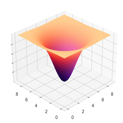
Figure 1: Visualization of the bivariate density function with X = Y = 4.5.

At each time step, an agent evaluates the gradient of its current position on the xy-plane based on the underlying density function with

$$\chi_{i,t}=\frac{f(x_{i,t}+\delta,y_{i,t})-f(x_{i,t}-\delta,y_{i,t})}{2\delta}-\lambda_{x,i,t}$$ (2)

$$\psi_{i,t}=\frac{f(x_{i,t},y_{i,t}+\delta)-f(x_{i,t},y_{i,t}-\delta)}{2\delta}-\lambda_{y,i,t}$$ (3)

where $\delta$ is a fixed base step size and $\lambda$ is a random value between $-\Lambda$ and $\Lambda$, introducing stochasticity in agent-movement. In the attraction state, the agent’s new coordinates are

$$x_{{}_{i,t+1}},y_{{}_{i,t+1}}=x_{{}_{i,t}}+\chi_{{}_{i,t}},y_{{}_{i,t}}+\psi_{{}_{i,t}}$$ (4)

and in the repulsion state, they are

$$x_{{}_{i,t+1}},y_{{}_{i,t+1}}=x_{{}_{i,t}}-\chi_{{}_{i,t}},y_{{}_{i,t}}-\psi_{{}_{i,t}}$$ (5)

under periodic boundary conditions. Agents switch to the repulsion state once they approached the center of the valley within a distance of 0.3 and switch back to attraction at a rate of $1/(3\eta)$. This dynamic switching mechanism allows for movement across the simulation space, resembling commute-like behavior, instead of the entire population remaining around the center for the entire simulation time. A snapshot of a realization of the ABM at $t=9$ can be found in Figure 2, showing a dense cluster of agents at the center, surrounded by less densely populated space.

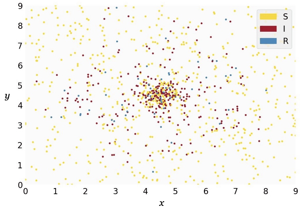
Figure 2: Snapshot ($t=9$) of a realization ABM variant B. Each point represents the position of a susceptible (yellow), infectious (red), or recovered (blue) agent.

3.1.2 Initialization

For initialization, agents are placed randomly across the simulation space in variant A. In variant B, initial positions and behavior states are determined using the Monte Carlo method, based on the bivariate density function for the coordinates, and $1/(1-1/3\eta)$ for the behavior state probabilities, and the outbreak starts after a burn-in period.

3.2 Sub-Model M2: Compartmental Model

The compartmental model follows the classic SIR (Susceptible-Infectious-Recovered) framework, describing the dynamics of disease spread in a population with ordinary differential equations (ODEs) [34, 5]. The model divides the population into three compartments: susceptible individuals ($S$), infectious individuals ($I$), and recovered individuals ($R$). The dynamics of the SIR model are governed by a system of ordinary differential equations (ODEs). The rate of change for each compartment is given by:

$$\frac{{dS}}{{dt}} =-\frac{{\beta\cdot S\cdot I}}{{N}}$$ (6)

$$\frac{{dI}}{{dt}} =\frac{{\beta\cdot S\cdot I}}{{N}}-\gamma\cdot I$$

$$\frac{{dR}}{{dt}} =\gamma\cdot I$$

where $\beta$ represents the transmission rate of the disease, $\gamma$ is the recovery rate, and $N$ is the total population size. This model captures the rates at which the population transitions between compartments. Given initial conditions, step size, and time frame, the ODEs can be solved numerically, providing compartment sizes over time - and thus simulating the dynamics of disease spread in a population.

3.3 Coupling

In the hybrid model, the population-space is spatially divided into an ABM (M1) and a compartmental region (M2), while allowing for population flow between regions. The interface between M1 and M2 is a vertical line that can be moved along the x-axis to adjust the proportions (or weight) of each model component. This flexible interface allows for varying the influence of each model within the hybrid framework.

The temporal resolution and the order of progresses can significantly impact the results of both ABMs and compartmental models [18]. This aspect is particularly crucial in our hybrid model due to the interaction between a discrete model and a continuous model [26]. To maintain coherence, time is implemented as a discrete variable in both models, and interactions within the ABM and between models occur synchronously. Figure 3 visualizes the coupling mechanism in the hybrid model, depicting the sequence of processes within a single time step.

The subsequent sections will detail these processes.

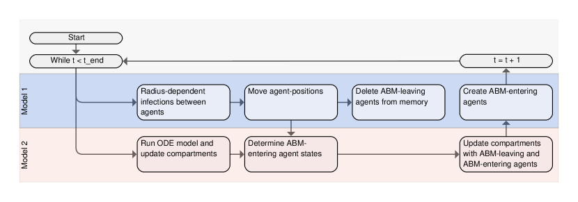
Figure 3: Order of processes in hybrid model.

3.3.1 Population flow between model regions

Agents can transition from the M1 (ABM) area to the M2 (ODE) area through the designated interface. Agents entering M2 are aggregated into $s_{in}$, $i_{in}$, and $r_{in}$, representing the number of susceptible, infectious, and recovered agents respectively. These agents are subsequently removed from the M1 population. Movement from M2 into M1 in a given time step is governed by the equation:

$$n_{out}(t)=s_{in}(t-1)+i_{in}(t-1)+r_{in}(t-1)$$ (7)

where $n_{out}$ is the number of agents leaving M2. This ensures that the flow between the two regions remains symmetric. The lag of one time step prevents scenarios where more agents leave M2 than are present, thus avoiding population inconsistencies. Since M2 does not simulate spatial movement the $y$-coordinate at which an agent leaves M2 is unknown. For variant A, this coordinate is sampled from a uniform distribution. For variant B, the marginal of the density function (see Equation 1) is used to derive sampling weights.

3.3.2 Infection dynamics within the ODE area

Due to population flow between models, the population size of M2 varies based on the incoming and outgoing agents. Additionally, the stochastic nature of the hybrid model requires a corrective procedure in M2 to ensure accurate population tracking and infection dynamics. This involves several steps:

First, the compartmental model described in Section 3.2 is solved for one time step with the current population size as shown in the following equations:

$$\Sigma_{1}(t+1) =S(t)-\frac{\beta\cdot S(t)\cdot I(t)}{N(t)}dt$$ (8)

$$\Phi_{1}(t+1) =I(t)+\frac{\beta\cdot S(t)\cdot I(t)}{N(t)}-\gamma\cdot I(t)dt$$

$$\Psi_{1}(t+1) =R(t)+\gamma\cdot I(t)dt$$

Next, the state of the leaving population is determined. The state of each leaving agent is drawn in a multinomial trial using the results from the previous step as the class probabilities:

$$s_{out}(t),i_{out}(t),r_{out}(t)\sim\textrm{Multinomial}\left(n_{out}(t),\left[\frac{\Sigma_{1}(t+1)}{N(t)},\frac{\Phi_{1}(t+1)}{N(t)},\frac{\Psi_{1}(t+1)}{N(t)}\right]\right)$$ (9)

The leaving population is then subtracted from each compartment, ensuring no negative sizes by constraining each value to zero or higher (for conciseness, we will demonstrate the following procedures for the S-compartment, but they also applied to the I- and R-compartment):

$$\Sigma_{2}(t+1) =\textrm{max}(0,\Sigma_{1}(t+1)-s_{out}(t))$$ (10)

Given this reduction, the sum of the compartments may exceed the actual remaining population, calculated as $N(t)-n_{out}(t)$. Therefore, a correction term $\kappa$ is computed to balance this discrepancy:

$$P(t+1) =\Sigma_{2}(t+1)+\Phi_{2}(t+1)+\Psi_{2}(t+1)$$ (11)

$$\kappa(t) =P(t+1)-(N(t)-n_{out}(t))$$

This correction term is proportionally subtracted from each compartment to ensure that their sum matches the actual population:

$$\Sigma_{3}(t+1) =\Sigma_{2}(t+1)-\kappa(t)\cdot\frac{\Sigma_{2}(t+1)}{P(t+1)}$$ (12)

As a final step, the entering population is added to the compartments, resulting in the final compartment sizes for the following time step:

$$S(t+1) =\Sigma_{3}(t+1)+s_{in}(t)$$ (13)

3.3.3 Parameter selection

To effectively compare and couple M1 and M2, both models need to produce similar epidemic outcomes given identical starting conditions. Following the procedure and disease characteristics in Breitwieser et al. [29], we first determine the parameters $\beta$ and $\gamma$ for M2, corresponding to a measles epidemic with $R_{0}=12.9$ and an 8-day recovery period, resulting in $\beta=1.61$ and $\gamma=1/8$. Next, we generate a time series of infectious individuals by numerically solving the compartmental model using initial values of $S=995,I=5,R=0$ and a step size of 0.33 days. This is achieved with the RK45 method, as implemented in SciPy’s integrate.solve_ivp function [35].

We then fit the parameters $\Lambda$, $\rho$, and $\theta$ for M1-A to match the time series data, with the same initial conditions and a recovery rate of $1/24$ (to correspond to a step size of 0.33 days). This optimization is done using the Nelder-Mead minimizer (as implemented in SciPy’s optimize.minimize [35]) with least squares as the cost function, yielding $\Lambda=0.215$, $\rho=0.025$, and $\theta=1.162$.

We repeat the procedure for M1-B, and additionally fit the parameter $\delta$ (the base step size), fixing $\eta$ at 3, and positioning the attraction point at $X=Y=4.5$. This results in $\Lambda=0.268$, $\rho=0.016$, $\theta=1.01$, and $\delta=0.01$.

Figure 4 shows that M1-A and M2 produce closely aligned SIR curves, while M1-B exhibits a more rapid rise and a lower peak of infections. This is consistent with the finding in Susandi et al. [36] that ABMs with heterogeneous populations cannot produce identical results to compartmental models - which explains this discrepancy.

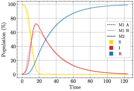
Figure 4: SIR curves for model 2 (solid lines) and the average results for 100 realizations of the fitted M1 variants A (dashed lines) and B (dotted lines).

In the following section, we describe the numerical experiments conducted to evaluate the performance and robustness of our hybrid modeling approach. The primary objective is to understand how varying the weight of the compartmental (ODE-based) and agent-based component affects model predictions, infection dynamics, and computational efficiency. By systematically adjusting these weights, we aim to uncover the nuanced behavior of the hybrid model under different configurations. This analysis will provide valuable insights into the potential applications and limitations of the suggested hybrid model in infectious disease modeling.

4 Experimental Setup and Methodology

In this section, we describe the experimental setup and methodology used to evaluate the fundamental dynamics of our hybrid model. By varying the weight between its two main components - the agent-based model (M1) and the compartmental model (M2) - we aim to understand how altering the balance between these components and the location of the interface affects the model outcomes in terms of the infectious wave. This setup allows us to test the robustness of our model under various conditions. The results of these experiments are presented in the subsequent section.

4.1 Model Weights

We adjust the weights of M1 ($w_{1}$) and M2 ($w_{2}$) by shifting the interface in the hybrid model along the x-axis. For example, given $0\leq x\leq 9$, placing the interface at x=4.5 results in $w_{1}=w_{2}=0.5$, while a placement at x=6.75 results in $w_{1}=0.25$ and $w_{2}=0.75$. The interface shift allows us to systematically study the impact of different model configurations on infection dynamics.

4.2 Model Configurations

We compare two configurations of the hybrid model: Hybrid Model A (M1-A with M2) and Hybrid Model B (M1-B with M2). This comparison allows us to examine our hybrid model under two scenarios. In the first scenario (Hybrid Model A), both model components simulate a homogeneous population, leading to very similar results individually. In the second scenario (Hybrid Model B), the agent-based component simulates a heterogeneous population, yielding different epidemic dynamics compared to the M2-component. In this scenario, the attraction point is placed at the center of the simulation space $(x=4.5,y=4.5)$, making the distance of the attraction point to the interface dependent on $w$. For $w_{2}>0.5$, the attraction point is located within the borders of M2. Additionally, we examine a third scenario in the appendix, where the location of the attraction point is always placed at the center of M1, rather than at the center of the full simulation space. These scenarios enable us to study the implications of spatial differences on spatial coupling effects.

4.3 Evaluation Metrics

For the experiments, we evaluate the following metrics for the resulting time series of the infectious population: (a) the root mean squared error (RMSE) compared to the baseline from M2; (b) the peak height; (c) the time step at which the peak occurs; (d) the Fisher-Pearson coefficient of skewness, indicating the buildup speed of the infectious wave; (e) the full-width-at-half-maximum (FWHM), indicating the sharpness of the peak. The RMSE quantifies the overall deviation from the reference model, while metrics b$\ldots$e provide detailed insights into the dynamics and shape of the epidemic. Finally, we measure (f) the average CPU time for each model configuration. We increase the weight of M2 from 0 to 1 in 0.02 steps, averaging the metrics after 100 independent realizations per configuration.

5 Results

This section presents the results of our experiments, evaluating the performance and robustness of the hybrid model under different configurations. Specifically, we examine how varying the weight of the compartmental model (M2) and the agent-based model (M1) affects various metrics (see previous section) related to infection dynamics and computational efficiency in both Hybrid Model A (M1-A with M2) and Hybrid Model B (M1-B with M2).

Results are shown in Figures 5(a)-5(f) for Hybrid Model A and in Figures 6(a)-6(f) for Hybrid Model B. The x-axis represents the weight of M2 ($w_{2}$). When $w_{2}=0$, the entire population is modeled by M1, and when $w_{2}=1$, the entire population is modeled by M2.

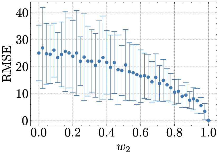
(a)

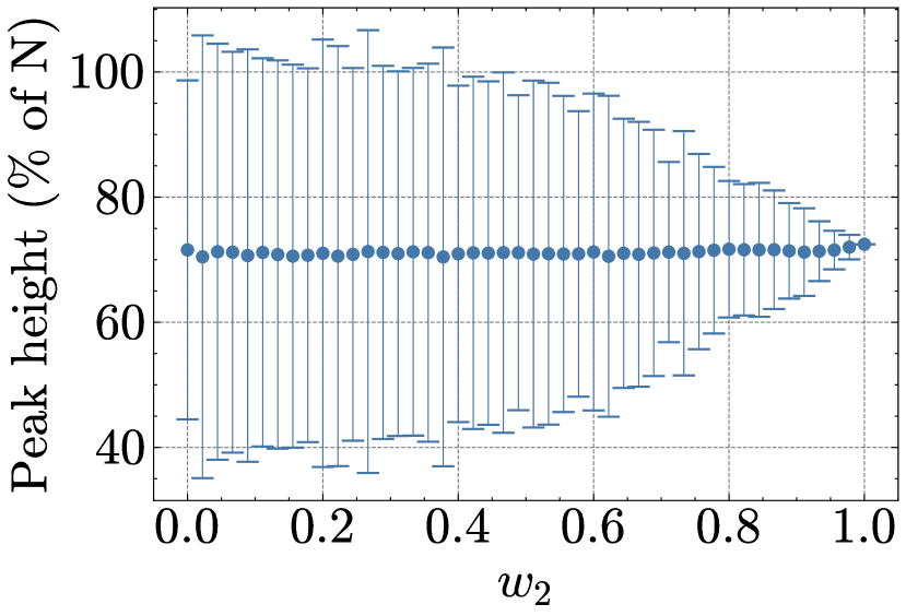
(b)

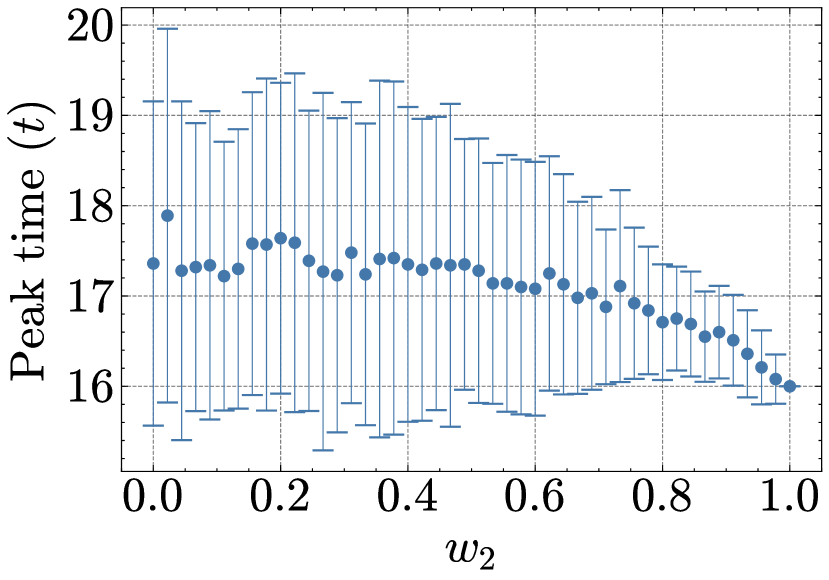
(c)

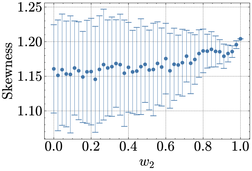
(d)

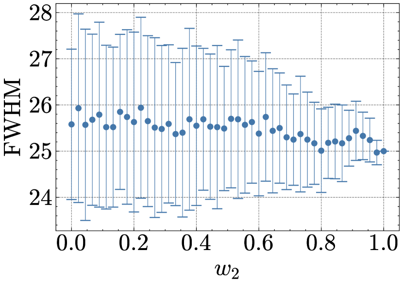
(e)

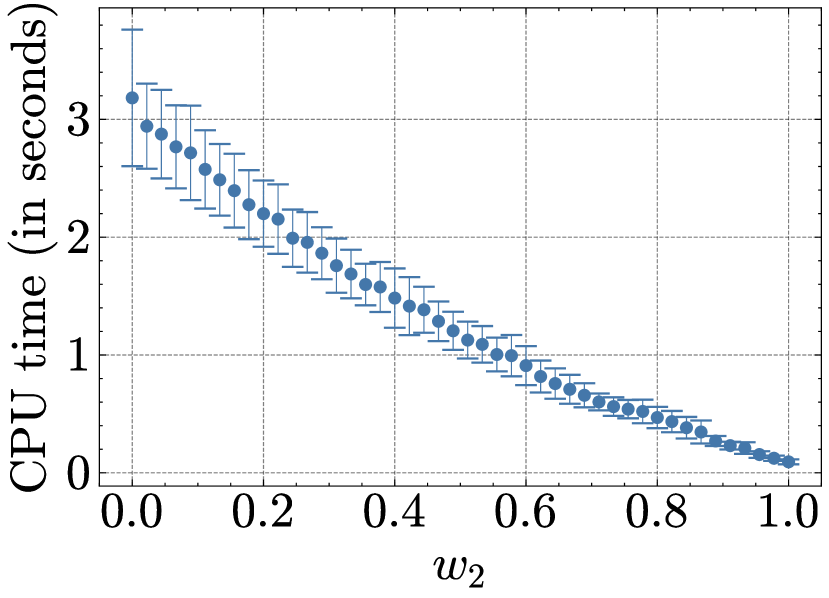
(f)

Figure 5: Hybrid model A: Average results for 100 independent realizations per level of model 2 weight ($w_{2}$). Bars around points represent the standard deviation. (a) RMSE for the time series of infectious between the reference model and the hybrid model. (b) Peak time of the time series of infectious. (c) Peak height of the time series of infectious. (d) Fisher-Pearson coefficient of skewness of the time series of infectious. (e) FWHM of the time series of infectious. (f) CPU time in seconds.

5.1 Hybrid model A

5.1.1 Root Mean Squared Error (RMSE)

The RMSE for different weights behaves as expected, showing a steady drop from 25.09 to 0 as the weight of the M2-component increases. This is because the full M2-model serves as the reference model to compute the RMSE. The standard deviation is larger for lower values of $w_{2}$, which is due to the stochastic nature of M1.

5.1.2 Peak height

The peak height of the infection curve does not change significantly with changing $w_{2}$. It remains around 71.57% at $w_{2}=0$ and 72.46% at $w_{2}=1$. This consistency is expected since the peak height is similar in both individual models M1-A and M2, as shown in 4. Similar to the RMSE, the standard deviation shrinks with increasing $w_{2}$.

5.1.3 Peak time

A notable coupling effect is observed in the peak time of the infectious curve. While the peak time is slightly earlier in the reference model ($16t$) compared to M1-A ($17.36t$), it does not gradually decrease as $w_{2}$ increases. Instead, there seems to be a quadratic relationship between the peak time and $w_{2}$. This may be due the discrete implementation of time in our models and the relatively small difference in peak time of 1.36 time steps between the model components, causing the resulting peak time to align more closely with the model component modeling the majority of the population.

5.1.4 Skewness

The skewness coefficient is 1.16 at $w_{2}=0$ and 1.2 at $w_{2}=1$, indicating slightly more weight on the right tail of the infectious wave in M2 compared to M1-A. The quadratic relationship in peak time is reflected in the skewness, which increases more rapidly as $w_{2}$ exceeds the 0.6-mark, likely due to the peak time influencing the skewness of the infectious wave.

5.1.5 Full-Width-at-Half-Maximum (FWHM)

The FWHM is 25.58 at $w_{2}=0$ and 25 at $w_{2}=1$, indicating that the infectious wave of M2 is sharper compared to M1. However, this difference is minor and steadily decreases as $w_{2}$ increases, suggesting minimal coupling effects.

5.1.6 CPU time

The CPU time decreases from 3.18 to 0.09 seconds as $w_{2}$ increases, following a convex pattern. This diminishing reduction in CPU time can be attributed to the stochastic processes computed for each agent, where calculations often involve interactions with all other agents. Thus, the reduction in computational load is more substantial when increasing $w_{2}$ from lower values (e.g., 0 to 0.02) compared to higher values (e.g., 0.9 to 0.92), reflecting the non-linear scaling of interaction complexity.

5.2 Hybrid model B

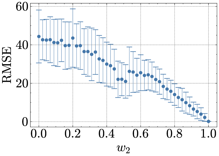
(a)

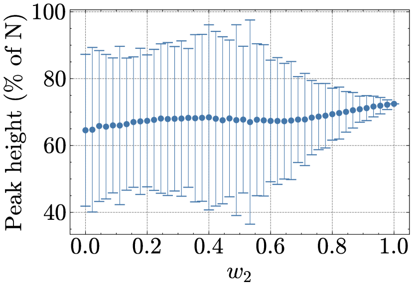
(b)

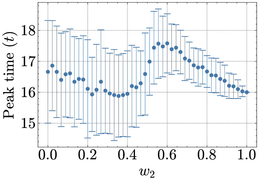
(c)

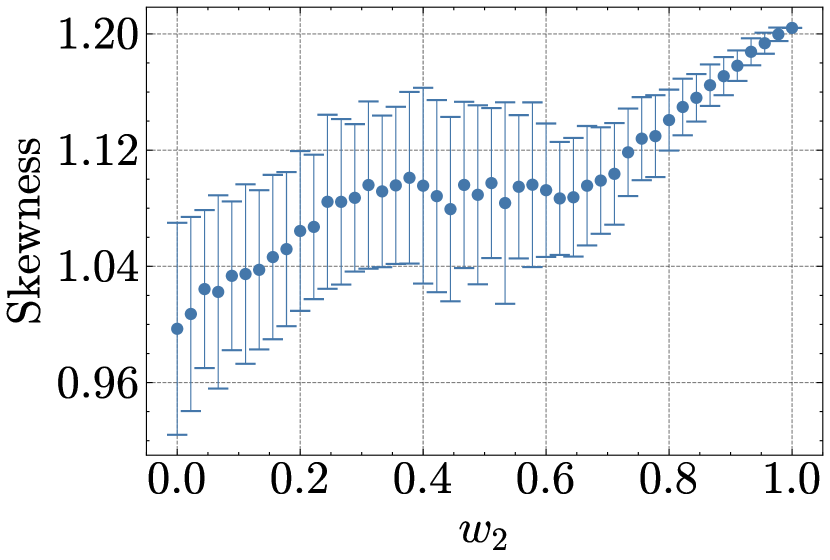
(d)

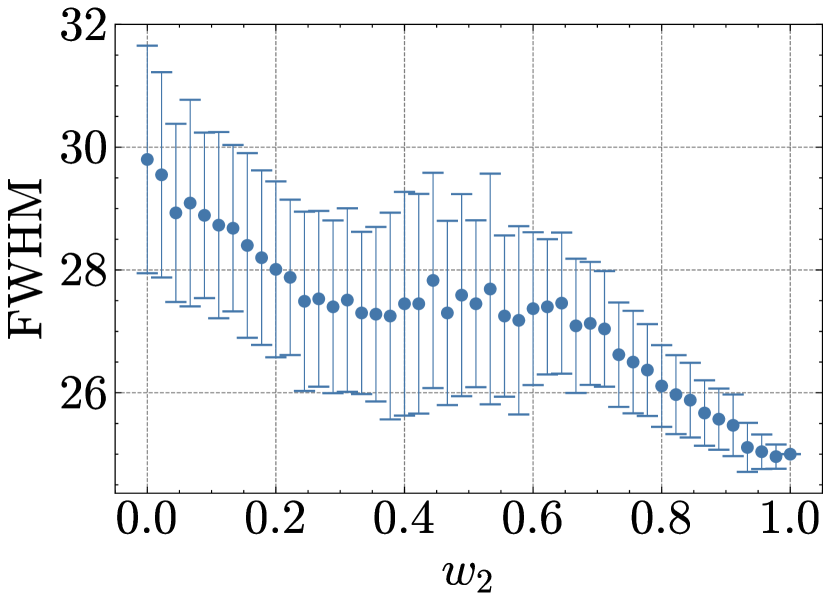
(e)

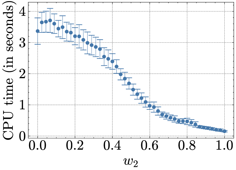
(f)

Figure 6: Hybrid model B: Average results for 100 independent realizations per level of model 2 weight ($w_{2}$). Bars around points represent the standard deviation. (a) RMSE for the time series of infectious between the reference model and the hybrid model. (b) Peak time of the time series of infectious. (c) Peak height of the time series of infectious. (d) Fisher-Pearson coefficient of skewness of the time series of infectious. (e) FWHM of the time series of infectious. (f) CPU time in seconds.

5.2.1 Root Mean Squared Error (RMSE)

The RMSE at $w_{2}=0$ is 44.3, nearly twice as large as the RMSE for M1-A. Similar to Hybrid Model A, the RMSE for Hybrid Model B drops towards zero as $w_{2}$ increases. However, there is a notable minimum around the 0.5-mark of $w_{2}$. The RMSE decreases for $w_{2}$ values below 0.5, then increases for $w_{2}$ values above 0.5 before dropping again after the 0.6-mark. This indicates that M2 has a stronger effect on model results around the 0.5 mark than at the 0.6 mark. This can be attributed to the attraction point in the agent-based component, resulting in a spatially heterogeneous population. Agents form a cluster where the infection spreads more rapidly. When $w_{2}$ is set to 0.5, the attraction point lies on the interface between M1-B and M2, attracting many agents into M2 and therefore increasing the interaction between the models.

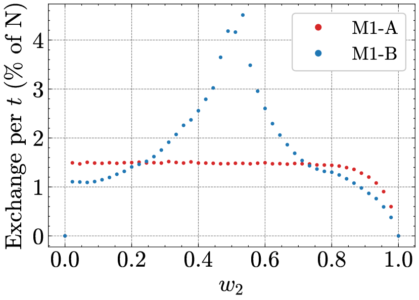
(a)

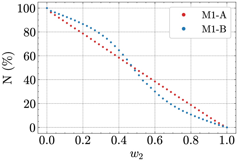
(b)

Figure 7: Changes in population metrics for Hybrid Model A and B for different weights of M2. Results from 100 independent realizations. (a) Average percentage of population entering M2 per $t$. (b) Average percentage of overall population in M1 per $t$.

Indeed, Figure 7(a) shows that the average population flow from M1 to M2 during a time step depends on $w_{2}$. In Hybrid Model A, it is around 1.5% of the total population for weights below 0.8, before dropping for higher weights. In Hybrid Model B, it increases from 0.02 to 0.53, peaking at 4.5%, before decreasing rapidly for higher weights. Additionally, Figure 7(b) shows that the share of the overall population present in M1 drops faster around $w=0.5$ in Hybrid Model B, while decreasing steadily in Hybrid Model A.

5.2.2 Peak height

The peak height of M1-B is 64.56%, considerably lower than in M2. A notable observation is the increased standard error around the 0.5-mark of $w_{2}$, reflecting the increased between-model interaction discussed earlier. The peak height follows a convex pattern: For $w_{2}<0.4$, the average peak height increases towards the higher value of M2, but decreases after the 0.4-mark until $w_{2}=0.6$. This pattern suggests that the attraction point’s proximity to the interface significantly influences infection dynamics.

5.2.3 Peak time

The peak time of a full M1-B is $16.66t$ (at $w_{2}=0$), slightly closer to the reference model than M1-A. The attraction point appears to influence the peak time of the hybrid model. In the full M1-B model, the peak is delayed by 0.66 compared to M2. In Hybrid Model B, the peak time is closer to the full M2 result around $w_{2}=0.4$ than around $w_{2}=0.6$, again likely due to the increased between-model interaction around the 0.5-mark. The local minimum around the 0.4 mark, rather than the 0.5 mark, suggests that the discrete nature of time amplifies the interaction effect between the model components.

5.2.4 Skewness

The skewness of the resulting infectious data is considerably lower in M1-B than in M2, indicating a more symmetrical infection wave in M1-B. Although skewness increases with an increasing $w_{2}$, a local maximum at $w_{2}=0.38$ is followed by a minor drop until $w_{2}=0.64$. This reflects the shift observed in the previous metrics for Hybrid Model B.

5.2.5 Full-Width-at-Half-Maximum (FWHM)

At $w_{2}=0$, the FWHM is considerably higher (29.8) than at $w_{2}=1$ (25.0), indicating that the infectious peak of M1-B is more truncated than in M1-A or M2. Similar to the previous metric, a regression can be observed as $w_{2}$ increases with a temporary shift after the 0.38-mark. Both observations are consistent with the increased between-model exchange around this value.

5.2.6 CPU time

For lower $w_{2}$-values, the average CPU time of Hybrid Model B is higher than in the case of Hybrid Model A, at 3.37 seconds when $w_{2}=0$. This is due to the increased complexity introduced by the attraction points. Additionally, there is an increase from $w_{2}=0$ to $w_{2}=0.06$, possibly due to the further complexity introduced by population flow from M2 to M1, influenced by the landscape in M1. For Hybrid Model B, the drop in CPU time follows the drop in population size of the M1-B component, as visualized in Figure 7(b). The computational demands of M1 stem from simulating each individual agent, making the population size a key factor in determining CPU time.

6 Discussion

The results for Hybrid Model A demonstrate that the outcomes are directly proportional to the weighting of each model component. Specifically, as the weighting shifts, the model’s outcomes increasingly resemble the results of the predominant component. This proportional relationship indicates that the hybrid model effectively balances the computational efficiency of the compartmental model (M2) with the detailed interactions of the agent-based model (M1-A). By adjusting the weight between these components, the hybrid model can be fine-tuned to optimize either efficiency or detail, providing a versatile and scalable approach to infectious disease modeling.

In contrast, the results for Hybrid Model B reveal a more complex interaction involving the implemented attraction point and the between-model interface. This interaction triggers switches in the model outcomes, favoring one component over the other under different conditions. The direction-switching effect observed in the peak time and peak height for Hybrid Model B can be explained by the presence of the attraction point. Without the attraction point, these metrics would likely follow a trajectory similar to Hybrid Model A. However, the increased between-model interaction around $w_{2}=0.5$ leads to a local change, emphasizing the sensitivity of the hybrid model to the spatial configuration of the attraction point.

6.1 Impact on Infection Spread Dynamics

The study reveals that spatial coupling of an ABM with an ODE-based model can effectively capture the dynamics of infection spread in the overall population. In Hybrid Model A, where both components simulate a homogeneous population, the infection dynamics transition smoothly as the weight shifts between M1 and M2. This smooth transition reflects a successful integration of the detailed agent interactions in M1 with the aggregate population-level processes in M2, maintaining consistency in the model’s outcomes.

In Hybrid Model B, where the agent-based component includes spatial heterogeneity, the infection dynamics reveal a deeper complexity. The presence of an attraction point introduces a non-uniform distribution of agents, leading to varied infection dynamics depending on the location of the interface. This demonstrates that spatial factors and agent clustering can significantly influence the spread of infection, underscoring the model’s ability to adapt to complex scenarios by accurately reflecting the impact of spatial configurations and agent movements.

These findings highlight that the location of the coupling mechanism in a hybrid model can amplify the differences between model components. Differences between models and sub-populations, as well as the level of population flow, should be carefully considered in real-world applications. The increased between-model interaction observed in Hybrid Model B underscores the need for a nuanced approach to spatial coupling, especially when dealing with heterogeneous populations, thereby enhancing the model’s applicability and precision in various scenarios.

6.2 Computational Efficiency

Our experiments also provide insights into the computational efficiency of the hybrid model compared to a pure ABM. For Hybrid Model A, the hybrid approach achieves a substantial reduction in CPU time while maintaining accuracy in the infection dynamics. The proportional relationship between the weight of the compartmental model and the CPU time underscores the potential for significant computational savings. This is particularly beneficial in large-scale simulations where computational resources are a critical constraint.

In Hybrid Model B, while the overall trend shows reduced CPU time with increasing weight of the compartmental model, the relationship is more complex. The initial increase in CPU time at low values of $w_{2}$ reflects the added complexity due to the attraction point and the increased interaction between the models. Despite this complexity, the hybrid model still demonstrates a net reduction in computational cost compared to a pure ABM, especially at higher values of $w_{2}$. This indicates that even with added spatial heterogeneity, the hybrid model can offer computational advantages, though the exact savings depend on the specific configuration and interaction dynamics.

6.3 Limitations and Future Directions

One limitation of the hybrid model, compared to a pure ABM, is the loss of information during each exchange between the two model components. Whenever population flow from M2 to M1 is modeled, new agents are created and their individual statuses are randomly distributed based on the population’s current state. Consequently, an agent that recently entered M2 as recovered may effectively leave as susceptible or infectious. Exploring alternative strategies for information exchange between the models and refining the coupling mechanism could potentially address this limitation and improve the accuracy of the hybrid model in capturing individual-level dynamics.

Overall, these findings provide valuable insights into the strengths and limitations of hybrid modeling approaches. They emphasize the importance of carefully considering the spatial configuration and interaction dynamics between model components to optimize both accuracy and computational efficiency. Future research could focus on developing more sophisticated coupling mechanisms and exploring the application of hybrid models to a broader range of infectious diseases and real-world scenarios.

7 Conclusion

In this paper, we addressed a significant research gap by introducing a novel spatial hybrid modeling approach that integrates a microscopic agent-based model (ABM) with a macroscopic compartmental ordinary differential equation (ODE) model. This topic has been scarcely explored in the existing literature on hybrid models. Our primary aim was to explore the potential of this hybrid model in reducing computational costs while maintaining accurate and detailed infection dynamics. We demonstrated how such coupling can be effectively achieved, highlighting the potential of spatial coupling in real-world epidemic modeling, advancing the understanding of hybrid systems, and setting a foundation for future research in this domain.

To evaluate the effectiveness of our approach, we utilized several performance metrics to detect coupling effects on the resulting infectious disease dynamics. Our experiment with two toy scenarios revealed that the outcomes of the hybrid model depend on the similarity between the integrated models. In both scenarios, the ODE component lacked the spatial resolution of the ABM-component. However, in the first scenario, where both model components described a homogeneous population, the hybrid model produced the same infectious disease dynamics as the reference model. In the second scenario, we introduced spatial heterogeneity within the ABM by enabling non-random agent movement and localized clustering around an attraction point. The corresponding hybrid model showed that disease dynamics were influenced by the location of the between-model interface relative to the attraction point.

To address this, we suggest a meta-population approach for the ODE-component, which could provide spatial resolution and heterogeneity without significantly increasing computational demands. We also noted that the extreme variations in agent density in our toy examples may not be as pronounced in real-world applications, potentially mitigating concerns about model discrepancies.

To focus our analysis on the coupling effects, we intentionally simplified the model components, maintaining the standard Susceptible, Infectious, and Recovered (S, I, R) categories in both model components. This simplification allowed us to evaluate the impact of spatial interactions without the added complexity of more elaborate disease states or interactions. However, increasing the number of categories could further highlight the computational advantages of the hybrid approach compared to a purely microscopic approach. Future research will explore more realistic scenarios to further validate and enhance our proposed hybrid model.

In conclusion, our spatial hybrid modeling approach presents a promising avenue for studying infectious diseases and complex systems. It offers opportunities to refine model accuracy and optimize computational efficiency, paving the way for more sophisticated and practical applications in future research endeavors.

8 Implementation

The model is implemented in Python v3.9 [37] and the code is available on GitHub (http://github.com/iebos/hybrid_model1). The model includes three primary class objects: The Person class which creates an agent, the Model_ODE class which solves the ODEs and the Model_hybrid_realistic_continuous which creates the ABM and couples it to the ODE.

9 Acknowledgements

The work on the paper was funded by the German Ministry of research and education (BMBF) (project MODUS-Covid, grant number 031L0302C), and under Germany’s Excellence Strategy (MATH+ -The Berlin Mathematics Research Center, grant number EXC-2046/1, project no. 390685689, subproject EF45-4). The authors extend their gratitude to Kai Nagel and Kristina Maier for their valuable insights and comments on an early draft of this manuscript.

Appendix A Appendix 1

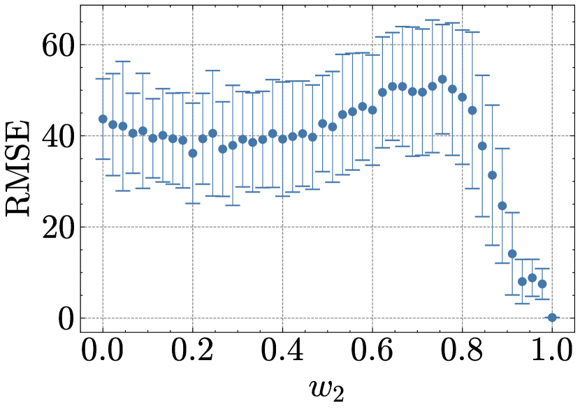
(a)

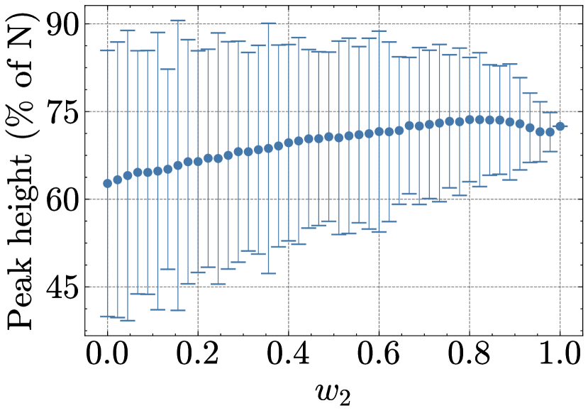
(b)

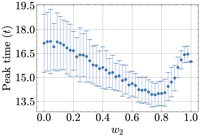
(c)

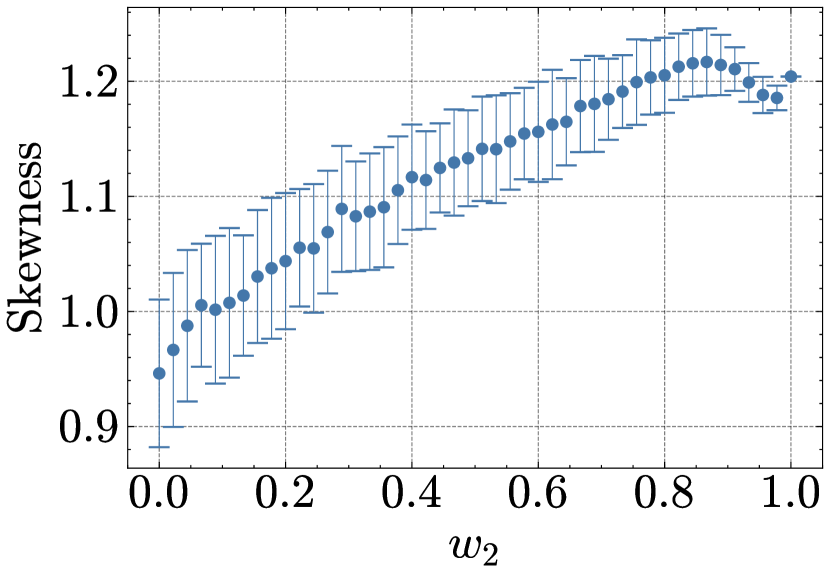
(d)

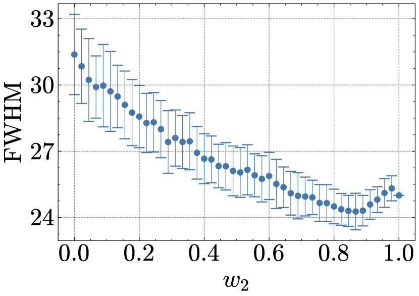
(e)

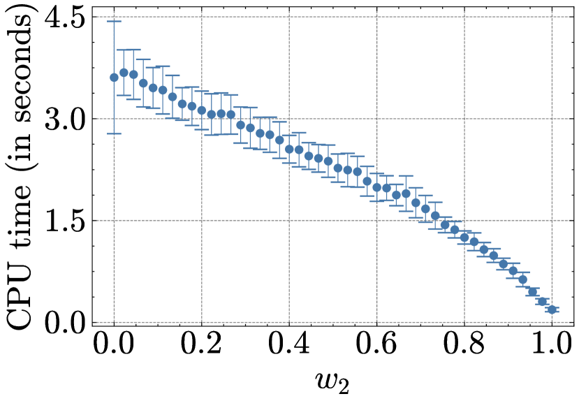
(f)

Figure 8: Hybrid model C: Average results for 100 independent realizations per level of model 2 weight ($w_{2}$). Bars around points represent the standard deviation. (a) RMSE for the time series of infectious between the reference model and the hybrid model. (b) Peak time of the time series of infectious. (c) Peak height of the time series of infectious. (d) Fisher-Pearson coefficient of skewness of the time series of infectious. (e) FWHM of the time series of infectious. (f) CPU time in seconds.

Figures 8(a) - 8(f) show results for Hybrid Model C, where the attraction point is placed at the center of M1. For example, at the pure ABM at $w_{2}=0$, it is at the same location as in Hybrid Model B at $(x=4.5,y=4.5)$. However, at $w_{2}=0.5$, it is placed at $(x=2.25,y=4.5)$. Most metrics behave differently than in results for Hybrid Model A and B. Rather than a steady or irregular trend towards the value of the reference model, most metrics rapidly increase or decrease towards the direction of the reference model and exceed or precede the reference value around $w_{2}=0.8$, before regressing towards it again. Most notably, the RMSE increases from $w_{2}=0.2$ to $w_{2}=0.74$ before sharply dropping. Given that the location of the attraction point can affect the population density within M1 and also the overall population distribution between the model components, it is likely that the fitted parameters of the pure ABM are not appropriate under these different conditions. Further, while the attraction point remains within M1, the distance to the interface grows smaller with increasing $w_{2}$. Figure 9(a) shows that as a result, between-model interaction increases continuously rather than peaking around the middle as is the case in Hybrid Model B. Additionally, Figure 9(b) shows that the majority of the overall population is located within M1 for $w_{2}<0.85$. Therefore, for Hybrid Model C, the weight of M2 is not a sufficient indicator of the influence of M2 on overall population dynamics.

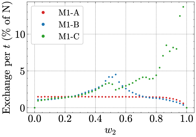
(a)

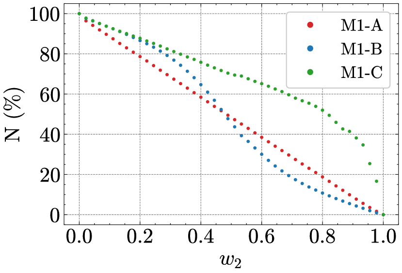
(b)

Figure 9: Changes in population metrics for Hybrid Model A, B, and C for different weights of M2. Results from 100 independent realizations. (a) Average percentage of population entering M2 per $t$. (b) Average percentage of overall population in M1 per $t$.

References

- Lancet Comission [2024] Lancet Comission. How modelling can better support public health policy making: the Lancet Commission on Strengthening the Use of Epidemiological Modelling of Emerging and Pandemic Infectious Diseases. The Lancet, 403(10429):789–791, March 2024. ISSN 01406736. doi: 10.1016/S0140-6736(23)02758-7. URL https://linkinghub.elsevier.com/retrieve/pii/S0140673623027587.
- Skrip and Townsend [2019] Laura A. Skrip and Jeffrey P. Townsend. Modeling Approaches Toward Understanding Infectious Disease Transmission. In Peter J. Krause, Paula B. Kavathas, and Nancy H. Ruddle, editors, Immunoepidemiology, pages 227–243. Springer International Publishing, Cham, 2019. ISBN 978-3-030-25552-7 978-3-030-25553-4. doi: 10.1007/978-3-030-25553-4_14. URL http://link.springer.com/10.1007/978-3-030-25553-4_14.
- Becker et al. [2021] Alexander D Becker, Kyra H Grantz, Sonia T Hegde, Sophie Bérubé, Derek A T Cummings, and Amy Wesolowski. Development and dissemination of infectious disease dynamic transmission models during the COVID-19 pandemic: what can we learn from other pathogens and how can we move forward? The Lancet Digital Health, 3(1):e41–e50, January 2021. ISSN 25897500. doi: 10.1016/S2589-7500(20)30268-5. URL https://linkinghub.elsevier.com/retrieve/pii/S2589750020302685.
- Hethcote [2000] Herbert W. Hethcote. The Mathematics of Infectious Diseases. SIAM Review, 42(4):599–653, 2000. doi: 10.1137/S0036144500371907. URL https://doi.org/10.1137/S0036144500371907. _eprint: https://doi.org/10.1137/S0036144500371907.
- Brauer et al. [2019] Fred Brauer, Carlos Castillo-Chavez, and Zhilan Feng. Mathematical Models in Epidemiology, volume 69 of Texts in Applied Mathematics. Springer New York, New York, NY, 2019. ISBN 978-1-4939-9826-5 978-1-4939-9828-9. doi: 10.1007/978-1-4939-9828-9. URL https://link.springer.com/10.1007/978-1-4939-9828-9.
- Duan et al. [2015] Wei Duan, Zongchen Fan, Peng Zhang, Gang Guo, and Xiaogang Qiu. Mathematical and computational approaches to epidemic modeling: a comprehensive review. Frontiers of Computer Science, 9(5):806–826, October 2015. ISSN 2095-2228, 2095-2236. doi: 10.1007/s11704-014-3369-2. URL http://link.springer.com/10.1007/s11704-014-3369-2.
- Wulkow et al. [2021] Hanna Wulkow, Tim O. F. Conrad, Nataša Djurdjevac Conrad, Sebastian A. Müller, Kai Nagel, and Christof Schütte. Prediction of Covid-19 spreading and optimal coordination of counter-measures: From microscopic to macroscopic models to Pareto fronts. PLOS ONE, 16(4):e0249676, April 2021. ISSN 1932-6203. doi: 10.1371/journal.pone.0249676. URL https://dx.plos.org/10.1371/journal.pone.0249676.
- Chang et al. [2021] Serina Chang, Emma Pierson, Pang Wei Koh, Jaline Gerardin, Beth Redbird, David Grusky, and Jure Leskovec. Mobility network models of COVID-19 explain inequities and inform reopening. Nature, 589(7840):82–87, January 2021. ISSN 0028-0836, 1476-4687. doi: 10.1038/s41586-020-2923-3. URL http://www.nature.com/articles/s41586-020-2923-3.
- Calvetti et al. [2020] Daniela Calvetti, Alexander P. Hoover, Johnie Rose, and Erkki Somersalo. Metapopulation Network Models for Understanding, Predicting, and Managing the Coronavirus Disease COVID-19. Frontiers in Physics, 8:261, June 2020. ISSN 2296-424X. doi: 10.3389/fphy.2020.00261. URL https://www.frontiersin.org/article/10.3389/fphy.2020.00261/full.
- Winkelmann et al. [2021] Stefanie Winkelmann, Johannes Zonker, Christof Schütte, and Nataša Djurdjevac Conrad. Mathematical modeling of spatio-temporal population dynamics and application to epidemic spreading. Mathematical Biosciences, 336:108619, June 2021. ISSN 00255564. doi: 10.1016/j.mbs.2021.108619. URL https://linkinghub.elsevier.com/retrieve/pii/S0025556421000614.
- Gao et al. [2022] Shupeng Gao, Xiangfeng Dai, Lin Wang, Nicola Perra, and Zhen Wang. Epidemic Spreading in Metapopulation Networks Coupled With Awareness Propagation. IEEE Transactions on Cybernetics, pages 1–13, 2022. ISSN 2168-2267, 2168-2275. doi: 10.1109/TCYB.2022.3198732. URL https://ieeexplore.ieee.org/document/9875017/.
- Railsback and Grimm [2019] Steven F. Railsback and Volker Grimm. Agent-based and individual-based modeling: a practical introduction. Princeton University Press, Princeton ; Oxford, second edition edition, 2019. ISBN 978-0-691-19082-2 978-0-691-19083-9. OCLC: on1051137181.
- Bruch and Atwell [2015] Elizabeth Bruch and Jon Atwell. Agent-Based Models in Empirical Social Research. Sociological Methods & Research, 44(2):186–221, May 2015. ISSN 0049-1241, 1552-8294. doi: 10.1177/0049124113506405. URL http://journals.sagepub.com/doi/10.1177/0049124113506405.
- Kerr et al. [2021] Cliff C. Kerr, Robyn M. Stuart, Dina Mistry, Romesh G. Abeysuriya, Katherine Rosenfeld, Gregory R. Hart, Rafael C. Núñez, Jamie A. Cohen, Prashanth Selvaraj, Brittany Hagedorn, Lauren George, Michał Jastrzębski, Amanda S. Izzo, Greer Fowler, Anna Palmer, Dominic Delport, Nick Scott, Sherrie L. Kelly, Caroline S. Bennette, Bradley G. Wagner, Stewart T. Chang, Assaf P. Oron, Edward A. Wenger, Jasmina Panovska-Griffiths, Michael Famulare, and Daniel J. Klein. Covasim: An agent-based model of COVID-19 dynamics and interventions. PLOS Computational Biology, 17(7):e1009149, July 2021. ISSN 1553-7358. doi: 10.1371/journal.pcbi.1009149. URL https://dx.plos.org/10.1371/journal.pcbi.1009149.
- Arifin et al. [2015] S. M. Niaz Arifin, Rumana Reaz Arifin, Dilkushi De Alwis Pitts, M. Sohel Rahman, Sara Nowreen, Gregory R. Madey, and Frank H. Collins. Landscape Epidemiology Modeling Using an Agent-Based Model and a Geographic Information System. Land, 4(2):378–412, 2015. ISSN 2073-445X. doi: 10.3390/land4020378. URL https://www.mdpi.com/2073-445X/4/2/378.
- Müller et al. [2021] Sebastian A. Müller, Michael Balmer, William Charlton, Ricardo Ewert, Andreas Neumann, Christian Rakow, Tilmann Schlenther, and Kai Nagel. Predicting the effects of COVID-19 related interventions in urban settings by combining activity-based modelling, agent-based simulation, and mobile phone data. PLOS ONE, 16(10):e0259037, October 2021. ISSN 1932-6203. doi: 10.1371/journal.pone.0259037. URL https://dx.plos.org/10.1371/journal.pone.0259037.
- Merler et al. [2015] Stefano Merler, Marco Ajelli, Laura Fumanelli, Marcelo F C Gomes, Ana Pastore Y Piontti, Luca Rossi, Dennis L Chao, Ira M Longini, M Elizabeth Halloran, and Alessandro Vespignani. Spatiotemporal spread of the 2014 outbreak of Ebola virus disease in Liberia and the effectiveness of non-pharmaceutical interventions: a computational modelling analysis. The Lancet Infectious Diseases, 15(2):204–211, February 2015. ISSN 14733099. doi: 10.1016/S1473-3099(14)71074-6. URL https://linkinghub.elsevier.com/retrieve/pii/S1473309914710746.
- Özmen et al. [2016] Özgür Özmen, James J Nutaro, Laura L Pullum, and Arvind Ramanathan. Analyzing the impact of modeling choices and assumptions in compartmental epidemiological models. SIMULATION, 92(5):459–472, May 2016. ISSN 0037-5497, 1741-3133. doi: 10.1177/0037549716640877. URL http://journals.sagepub.com/doi/10.1177/0037549716640877.
- Hunter et al. [2018] Elizabeth Hunter, Brain Mac Mamee, and John D Kelleher. A Comparison of Agent-Based Models and Equation Based Models for Infectious Disease Epidemiology. In 26th AIAI Irish Conference on Artificial Intelligence and Cognitive Science, Dublin, 2018. doi: 10.21427/RTQ2-HS52. URL https://arrow.dit.ie/scschcomart/71/. Publisher: Technological University of Dublin.
- Bobashev et al. [2007] Georgiy V. Bobashev, D. Michael Goedecke, Feng Yu, and Joshua M. Epstein. A Hybrid Epidemic Model: Combining The Advantages Of Agent-Based And Equation-Based Approaches. In 2007 Winter Simulation Conference, pages 1532–1537, Washington, DC, USA, 2007. IEEE. ISBN 978-1-4244-1305-8. doi: 10.1109/WSC.2007.4419767. URL http://ieeexplore.ieee.org/document/4419767/.
- Hunter et al. [2020] Elizabeth Hunter, Brian Mac Namee, and John Kelleher. A Hybrid Agent-Based and Equation Based Model for the Spread of Infectious Diseases. Journal of Artificial Societies and Social Simulation, 23(4):14, 2020. ISSN 1460-7425. doi: 10.18564/jasss.4421. URL http://jasss.soc.surrey.ac.uk/23/4/14.html.
- Nghi et al. [2016] Huynh Quang Nghi, Tri Nguyen-Huu, Arnaud Grignard, Hiep Xuan Huynh, and Alexis Drogoul. Toward an Agent-Based and Equation-Based Coupling Framework. In Phan Cong Vinh and Leonard Barolli, editors, Nature of Computation and Communication, volume 168, pages 311–324. Springer International Publishing, Cham, 2016. ISBN 978-3-319-46908-9 978-3-319-46909-6. doi: 10.1007/978-3-319-46909-6_28. URL http://link.springer.com/10.1007/978-3-319-46909-6_28. Series Title: Lecture Notes of the Institute for Computer Sciences, Social Informatics and Telecommunications Engineering.
- Bradhurst et al. [2016] R.A. Bradhurst, S.E. Roche, I.J. East, P. Kwan, and M.G. Garner. Improving the computational efficiency of an agent-based spatiotemporal model of livestock disease spread and control. Environmental Modelling & Software, 77:1–12, March 2016. ISSN 13648152. doi: 10.1016/j.envsoft.2015.11.015. URL https://linkinghub.elsevier.com/retrieve/pii/S1364815215301043.
- Banos et al. [2015] Arnaud Banos, Nathalie Corson, Benoit Gaudou, Vincent Laperrière, and Sébastien Coyrehourcq. The Importance of Being Hybrid for Spatial Epidemic Models:A Multi-Scale Approach. Systems, 3(4):309–329, November 2015. ISSN 2079-8954. doi: 10.3390/systems3040309. URL http://www.mdpi.com/2079-8954/3/4/309.
- Marilleau et al. [2018] Nicolas Marilleau, Christophe Lang, and Patrick Giraudoux. Coupling agent-based with equation-based models to study spatially explicit megapopulation dynamics. Ecological Modelling, 384:34–42, September 2018. ISSN 03043800. doi: 10.1016/j.ecolmodel.2018.06.011. URL https://linkinghub.elsevier.com/retrieve/pii/S0304380018302163.
- Gustafsson and Sternad [2016] Leif Gustafsson and Mikael Sternad. A Guide to Population Modelling for Simulation. Open Journal of Modelling and Simulation, 04(02):55–92, 2016. ISSN 2327-4018, 2327-4026. doi: 10.4236/ojmsi.2016.42007. URL http://www.scirp.org/journal/doi.aspx?DOI=10.4236/ojmsi.2016.42007.
- Sewall et al. [2011] Jason Sewall, David Wilkie, and Ming C. Lin. Interactive hybrid simulation of large-scale traffic. In Proceedings of the 2011 SIGGRAPH Asia Conference, pages 1–12, Hong Kong China, December 2011. ACM. ISBN 978-1-4503-0807-6. doi: 10.1145/2024156.2024169. URL https://dl.acm.org/doi/10.1145/2024156.2024169.
- Frias-Martinez et al. [2011] Enrique Frias-Martinez, Graham Williamson, and Vanessa Frias-Martinez. An Agent-Based Model of Epidemic Spread Using Human Mobility and Social Network Information. In 2011 IEEE Third International Conference on Privacy, Security, Risk and Trust and 2011 IEEE Third International Conference on Social Computing, pages 57–64, Boston, MA, October 2011. IEEE. ISBN 978-1-4577-1931-8. doi: 10.1109/PASSAT/SocialCom.2011.142. URL https://ieeexplore.ieee.org/document/6113095/.
- Breitwieser et al. [2022] Lukas Breitwieser, Ahmad Hesam, Jean De Montigny, Vasileios Vavourakis, Alexandros Iosif, Jack Jennings, Marcus Kaiser, Marco Manca, Alberto Di Meglio, Zaid Al-Ars, Fons Rademakers, Onur Mutlu, and Roman Bauer. BioDynaMo: a modular platform for high-performance agent-based simulation. Bioinformatics, 38(2):453–460, January 2022. ISSN 1367-4803, 1367-4811. doi: 10.1093/bioinformatics/btab649. URL https://academic.oup.com/bioinformatics/article/38/2/453/6371176.
- Jones and Su [2015] Rachael M Jones and Yu-Min Su. Dose-response models for selected respiratory infectious agents: Bordetella pertussis, group a Streptococcus, rhinovirus and respiratory syncytial virus. BMC Infectious Diseases, 15(1):90, December 2015. ISSN 1471-2334. doi: 10.1186/s12879-015-0832-0. URL https://bmcinfectdis.biomedcentral.com/articles/10.1186/s12879-015-0832-0.
- Aganovic et al. [2023] Amar Aganovic, Guangyu Cao, Jarek Kurnitski, and Pawel Wargocki. New dose-response model and SARS-CoV-2 quanta emission rates for calculating the long-range airborne infection risk. Building and Environment, 228:109924, January 2023. ISSN 03601323. doi: 10.1016/j.buildenv.2022.109924. URL https://linkinghub.elsevier.com/retrieve/pii/S0360132322011544.
- Djurdjevac Conrad et al. [2018] Nataša Djurdjevac Conrad, Luzie Helfmann, Johannes Zonker, Stefanie Winkelmann, and Christof Schütte. Human mobility and innovation spreading in ancient times: a stochastic agent-based simulation approach. EPJ Data Science, 7(1):24, December 2018. ISSN 2193-1127. doi: 10.1140/epjds/s13688-018-0153-9. URL https://epjdatascience.springeropen.com/articles/10.1140/epjds/s13688-018-0153-9.
- Marshall and Duthie [2022] BM Marshall and AB Duthie. abmAnimalMovement: An R package for simulating animal movement using an agent-based model [version 1; peer review: 2 approved with reservations]. F1000Research, 11(1182), 2022. doi: 10.12688/f1000research.124810.1.
- Kermack et al. [1927] William Ogilvy Kermack, A. G. McKendrick, and Gilbert Thomas Walker. A contribution to the mathematical theory of epidemics. Proceedings of the Royal Society of London. Series A, Containing Papers of a Mathematical and Physical Character, 115(772):700–721, 1927. doi: 10.1098/rspa.1927.0118. URL https://royalsocietypublishing.org/doi/abs/10.1098/rspa.1927.0118. _eprint: https://royalsocietypublishing.org/doi/pdf/10.1098/rspa.1927.0118.
- Virtanen et al. [2020] Pauli Virtanen, Ralf Gommers, Travis E Oliphant, Matt Haberland, Tyler Reddy, David Cournapeau, Evgeni Burovski, Pearu Peterson, Warren Weckesser, Jonathan Bright, and others. SciPy 1.0: fundamental algorithms for scientific computing in Python. Nature methods, 17(3):261–272, 2020. Publisher: Nature Publishing Group.
- Susandi et al. [2021] Armi Susandi, Intan Taufik, Pingkan Aditiawati, and Sparisoma Viridi. The relation between agent-based model and susceptible-infected-recovered model for spread of disease. AIP Conference Proceedings, 2320(1):050032, March 2021. ISSN 0094-243X. doi: 10.1063/5.0038221. URL https://doi.org/10.1063/5.0038221. _eprint: https://pubs.aip.org/aip/acp/article-pdf/doi/10.1063/5.0038221/14227268/050032_1_online.pdf.
- Python Software Foundation [2020] Python Software Foundation. Python, 2020. URL https://www.python.org/. Archived at https://web.archive.org/web/20240718193634/https://www.python.org/.