Analysis of Polarized Dust Emission Using Data from the First Flight of Spider

Abstract

Using data from the first flight of Spider and from Planck HFI, we probe the properties of polarized emission from interstellar dust in the Spider observing region. Component separation algorithms operating in both the spatial and harmonic domains are applied to probe their consistency and to quantify modeling errors associated with their assumptions. Analyses spanning the full Spider region demonstrate that i) the spectral energy distribution of diffuse Galactic dust emission is broadly consistent with a modified-blackbody (MBB) model with a spectral index of $\beta_{\mathrm{d}}=1.45\pm 0.05$ $(1.47\pm 0.06)$ for $E$ ($B$)-mode polarization, slightly lower than that reported by Planck for the full sky; ii) its angular power spectrum is broadly consistent with a power law; and iii) there is no significant detection of line-of-sight decorrelation of the astrophysical polarization. The size of the Spider region further allows for a statistically meaningful analysis of the variation in foreground properties within it. Assuming a fixed dust temperature $T_{\mathrm{d}}=19.6$ K, an analysis of two independent sub-regions of that field results in inferred values of $\beta_{\mathrm{d}}=1.52\pm 0.06$ and $\beta_{\mathrm{d}}=1.09\pm 0.09$, which are inconsistent at the $3.9\,\sigma$ level. Furthermore, a joint analysis of Spider and Planck 217 and 353 GHz data within a subset of the Spider region is inconsistent with a simple MBB at more than $3\,\sigma$, assuming a common morphology of polarized dust emission over the full range of frequencies. These modeling uncertainties have a small—but non-negligible—impact on limits on the cosmological tensor-to-scalar ratio derived from the Spider dataset. The fidelity of the component separation approaches of future CMB polarization experiments may thus have a significant impact on their constraining power.

revtex4-1.clsrevtex4-2.cls tablenum SIXtablenum

1 Introduction

The polarization of the cosmic microwave background (CMB) contains a wealth of information about the contents, history, and origins of the Universe (Abazajian et al., 2016). Observations of the $E$-mode (“gradient”, scalar, even-parity) polarization pattern reveal details of acoustic oscillations in the primordial plasma. A measurement of a cosmological $B$-mode (“curl”, pseudoscalar, odd-parity) pattern on large angular scales would imply the presence of a background of primordial gravitational waves, and thus provide remarkable new insights into early Universe models (Kamionkowski & Kovetz, 2016; Seljak & Zaldarriaga, 1997).

Precision studies of CMB polarization are complicated by polarized emission at similar frequencies from foreground sources within our own Galaxy, notably synchrotron radiation and thermal emission from dust particles (Dunkley et al., 2009). Even at the highest Galactic latitudes, foreground emission is known to be far brighter than any primordial $B$-mode signal (BICEP2/Keck, Planck Collaborations et al., 2015). Observations at multiple frequencies can be used to differentiate CMB from foreground emission based upon their differing spectral energy distributions (SEDs) (Wright et al., 1991; Brandt et al., 1994). Several such component separation methods have been developed: see, e.g., Planck Collaboration et al. (2020a) and references therein. In order to stitch together such multi-frequency data, these methods must necessarily make assumptions about the nature of foregrounds: their spatial morphology, SED, or some combination thereof. Component separation is thus an imperfect process, and there are always some uncertainties due to these assumptions (Remazeilles et al., 2016; Hensley & Bull, 2018).

At frequencies above 100 GHz, Galactic dust emission is the dominant polarized foreground on large angular scales (Planck Collaboration, 2016). Dust grains, heated by stellar radiation to ${\sim}20$ K, thermally re-emit that energy with an efficiency that depends on the physical characteristics of the grains. Because emission is inefficient at wavelengths much larger than the grain itself, dust emissivity is expected to drop in the $mm$-wave regime where CMB measurements occur (Draine & Fraisse, 2009). Aspherical grains that are ferro- or para-magnetic will preferentially align relative to the local magnetic field, leading to linearly-polarized emission with large-scale correlations (Purcell, 1975). Motivated by this picture, it is common to model the dust SED as a thermal blackbody at temperature $T_{\mathrm{d}}$, modified by a power-law emissivity with exponent $\beta_{\mathrm{d}}$:

$$I(\nu)=\tau_{0}\left(\frac{\nu}{\nu_{0}}\right)^{\beta_{\mathrm{d}}}B(\nu,T_{\mathrm{d}}).$$ (1)

Here $B$ is the Planck spectrum for a blackbody emitter, $\nu_{0}$ is some reference frequency, and $\tau_{0}$ is the optical depth at the reference frequency. Equation 1 is referred to as a modified blackbody (MBB).

Though widely-used, this simple model is unlikely to reflect the full range of dust emission across the sky. The detailed nature of dust grains remains a subject of ongoing research (Hensley & Draine, 2022; Draine & Fraisse, 2009). Their composition, size distribution, and density are all expected to vary from place to place, as are their radiative and magnetic environments. Thus, we may naturally expect different dust populations in our Galaxy to exhibit different SEDs. Such variation of the spatial morphology of a foreground component with observation frequency—or, equivalently, of the component SED across the sky—is often called frequency decorrelation. Furthermore, observations of the CMB constitute a collection of line-of-sight (LOS) integrals through the materials surrounding us, each of which may traverse heterogeneous populations. In addition to complicating the dust SED, such LOS decorrelation can yield variation in polarization angle with frequency even within a single map pixel (Tassis & Pavlidou, 2015).

Decorrelation may significantly complicate efforts at component separation. For example, Poh & Dodelson (2017) have shown that naive extrapolation of dust templates made from 353 GHz data to lower frequencies can bias the recovery of the tensor-to-scalar ratio $r\leq 1.5\times 10^{-3}$. While an analysis by the BICEP team (BICEP/Keck Collaboration et al., 2023) showed no evidence of dust decorrelation within their observing region, there is evidence for its presence in larger regions. By identifying regions of the sky likely to contain magnetically misaligned clouds, Pelgrims et al. (2021) demonstrate that LOS frequency decorrelation is detectable within the Planck dataset, largely in the Northern Galactic cap. Ritacco et al. (2023) has further demonstrated LOS frequency decorrelation in large-scale regions close to the Galactic plane. It is thus critically important to test the assumptions behind common foreground separation techniques through detailed studies of dust polarization. Such studies will inform both the field of Galactic astrophysics as well as the prospects for foreground removal by future CMB experiments (Hensley et al., 2022; Hazumi et al., 2020; Abazajian et al., 2016).

This publication is part of a series describing results from the first flight of Spider, a balloon-borne CMB telescope optimized to search for $B$-modes on degree angular scales. These data from Spider provide a measurement of the angular power spectra of 4.8% of the polarized sky at two frequencies: 95 and 150 GHz (SPIDER Collaboration et al., 2022). Dust emission is the dominant foreground at these at these frequencies. Since the first Spider instrument did not include a channel optimized for dust, the analysis of these data relies heavily on Planck 217 and 353 GHz maps for component separation. The published $B$-mode results from these data relied primarily on template subtraction using the XFaster power spectrum estimator (Section 2.1) alongside comparisons with alternate estimators and foreground-cleaning techniques (e.g., Section 2.2).

This paper exploits the sensitivity and sky coverage of the Spider data to explore the properties of the Galactic emission and to quantify the impact of the methods and models employed on component separation. Section 2 reviews both component separation techniques, and in Section 3 they are applied to two distinct subsets of the Spider region to probe for evidence of spatial variation in the nature of the diffuse polarized dust emission. The fidelity of the MBB model is tested in a comparison of the results from the two sub-regions using two Planck-derived dust templates (353-100 GHz and 217-100 GHz). Section 4 examines different choices for modeling the dust SED within the full Spider region: the validity of the MBB model, the constancy of MBB parameters with angular scale, and the use of power-law models for the dust angular power spectrum. Section 5 searches for LOS decorrelation by developing a custom estimator to look for evidence of variation of dust polarization angle with frequency in the Spider observing region. Finally, Section 6 compares the measured dust power spectrum for this sky region to templates generated by the PySM foreground modeling package.

2 Component Separation Techniques

As in SPIDER Collaboration et al. (2022), our analyses in this paper rely on two main component separation techniques: foreground-template subtraction, and Spectral Matching Independent Component Analysis (SMICA). In this section, we present baseline versions of these methods. In Sections 3 and 4 we explore variations in the assumptions presented below in order to test our understanding of the polarized emission from interstellar dust.

2.1 Template Subtraction

In the baseline cosmological analysis of the Spider first flight data (SPIDER Collaboration et al., 2022), we remove polarized dust emission from the Spider 95 and 150 GHz maps by subtracting from them a scaled template for this emission derived from Planck data. The Spider implementation of foreground-template subtraction follows the approach pioneered by Page et al. (2007) in the analysis of the WMAP polarization data. Within any given map pixel observed at frequency $\nu$, the measured Stokes parameters, $S_{\nu}$, are each modeled as the sum of three components: CMB, dust, and noise:

$$S_{\nu}=S^{\,\mathrm{CMB}}+A_{\nu,\nu_{0}}S_{\nu_{0}}^{\,\mathrm{dust}}+n_{\nu}\,.$$ (2)

The uniform (pixel-independent) scaling factor $A_{\nu,\nu_{0}}$ connects the dust map at the observing frequency $\nu$ to that at the reference frequency $\nu_{0}=353$ GHz.

We construct our dust template by subtracting the Planck 100 GHz map from the 353 GHz map: $S_{\nu_{0}}^{\,\mathrm{t}}\equiv S_{\nu_{0}}-S_{100}$. Since the CMB component is independent of frequency in these units, this removes the CMB signal at the cost of a modest increase in noise. To produce a cleaned CMB map, we scale this dust template by a fitting parameter $\alpha$ and subtract it from $S_{\nu}$, giving

$$S_{\nu}-\alpha\,S_{\nu_{0}}^{\,\mathrm{t}} = S^{\,\mathrm{CMB}}+(A_{\nu,\nu_{0}}-\alpha\,[1-A_{100,\nu_{0}}])\,S_{\nu_{0}}^{\,\mathrm{dust}}$$ (3)

$$+ n_{\nu}-\alpha\,n_{\nu_{0}}^{\,\mathrm{t}}.$$

Here $n_{\nu}$ is the noise component at the frequency $\nu$, and $n_{\nu_{0}}^{\,\mathrm{t}}\equiv n_{\nu_{0}}-n_{100}$.

Following SPIDER Collaboration et al. (2022), we use the XFaster algorithm (Gambrel et al., 2021) to fit for values of $\alpha=A_{\nu,\nu_{0}}/(1-A_{100,\nu_{0}})$ and the tensor-to-scalar ratio, $r$, in a simultaneous fit to the Spider $EE$ and $BB$ spectra. Note that, before subtraction, the dust template is “reobserved,” i.e., injected as an input sky through the full Spider simulation pipeline; it is thus subjected to the same scan strategy, beam smoothing, time-domain filtering, and map-making as the sky observed by Spider. The reobserved template, like the Spider data, is corrected in map space for the temperature-to-polarization leakage induced by the pipeline.

The template method implements a single scalar-valued factor $\alpha$ for each Spider frequency multiplying the entire map. Thus, this method assumes that the morphology of the polarized dust emission is independent of frequency (at least between 353 GHz and 100 GHz) or, equivalently, that the dust SED is constant across the relevant sky area. Note, however, that this method does not impose assumptions on the dust SED itself. We will revisit this assumption in our analysis below, notably in Sections 3 and 5.

2.2 SMICA

Spectral Matching Independent Component Analysis (SMICA; Cardoso et al., 2008) is a method for constructing linear combinations among a collection of maps in order to isolate desired sky components (e.g., dust or CMB). In contrast to the map-space template analysis described above, SMICA operates in multipole space, acting on the spherical harmonic coefficients, $a_{\ell m}$, for each map. Given a collection of $n$ input frequency maps, we construct $\boldsymbol{Y}=(y_{1},\cdots,y_{n})$, where each $y_{i}$ is a row vector of $a_{\ell m}$ coefficients for a single map $i$. We use the SMICA algorithm to construct the column vector of map weights, $w$, such that the linear combination $s\equiv w^{T}\boldsymbol{Y}$ is an estimate of the spherical harmonic coefficients for our desired sky component. Throughout this section, lower case letters denote vectors, and upper case bold letters denote matrices.

The weights are optimized with respect to some model of the assumed sky components. Given a column vector, $a$, containing the frequency scaling of a given sky component across the various maps (uniform for CMB, MBB for dust), the multipole-binned weights, $w_{b}$, for this sky component are given by

$$w_{b}^{T}=\left(a^{T}\widetilde{\boldsymbol{R}}_{b}^{-1}a\right)^{-1}a^{T}\widetilde{\boldsymbol{R}}_{b}^{-1},$$ (4)

where $\widetilde{\boldsymbol{R}}_{b}$ is the binned modeled covariance matrix containing CMB, dust, and noise components. These weights minimize the variance of the reconstructed harmonic map, $\mathrm{var(s)}=w_{b}^{T}\widetilde{\boldsymbol{R}}_{b}w_{b}$ under the signal-preserving constraint $w_{b}^{T}a=1$ (Hurier et al., 2013).

When reconstructing component maps, each harmonic mode $a_{\ell m}$ is scaled by the corresponding $w_{b}$ for its appropriate bin. The reconstructed maps, $S$, are the inverse spherical harmonic transform of these weighted collections of harmonic modes.

SMICA’s power and flexibility lie in the freedom to impose (or relax) different assumptions about the components in this model, and thus about the relationships among the weights. As discussed in detail in SPIDER Collaboration et al. (2022), the SMICA implementation for the Spider $B$-mode analysis assumed a single dust component with a MBB SED. In this analysis we make two improvements to SMICA dust modeling: we do not impose an SED on the dust component, and we improve the power-spectrum estimation for the dust through a more accurate transfer function. Both changes are described further below.

In this analysis we do not assume a MBB dust SED, but instead fit for the dust $a$ as for any other parameter of the model defining $\widetilde{\boldsymbol{R}}_{b}$ (which includes the CMB, dust emission, and noise) using the same maximum-likelihood fitting procedure as in SPIDER Collaboration et al. (2022). We choose the arbitrary overall normalization of $a$ such that its 353 GHz element is set to 1. Fitting for the dust $a$ in this manner effectively trades precision for accuracy: the frequency-dependence of the reconstructed dust component will not be biased by any assumptions about the dust SED, but the uncertainty on the other fitted parameters (e.g., the amplitude of the emission) will likely be larger; it could be smaller, but only if the SED we would otherwise assume were an especially poor description of the data.

In previous analyses (SPIDER Collaboration et al., 2022), the sky components of $\widetilde{\boldsymbol{R}}_{b}$ are corrected for effects from filtering, beam smoothing, and mode-coupling kernels through a $J_{bb^{\prime}}$ transfer matrix, as per Leung et al. (2022). While this approach is accurate for CMB spectra, the different angular power spectrum of dust make it inaccurate for an unbiased recovery of the full-sky dust spectrum, especially at larger scales. In this paper we modify the model to apply $J_{bb^{\prime}}$ only to the CMB component, and instead apply a diagonal $F_{b}$ to the foreground component. $F_{b}$ is the ratio of the output to input power for each bin and is constructed from an ensemble of reobserved Gaussian dust realizations. These realizations follow a power-law scaling of amplitude with angular scale, with an exponent $\gamma=-2.30$, pivoting around $\ell=80$.

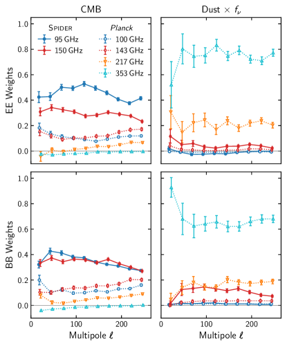
Figure 1: SMICA derived $EE$ (top) and $BB$ (bottom) weights to recover cleaned CMB (left) and dust (right) component $Q$/$U$ maps. The Spider 95 and 150 GHz maps contribute predominantly toward the CMB signal, recovered (dominant positive weights) in the left panels and removed (subdominant and/or negative weights) in the right panels. The Planck 217 and 353 GHz maps contribute predominantly toward the dust signal, removed in the left panels and recovered in the right panels. The dust weights are scaled with the fitted dust amplitude $f_{\nu}$ to indicate their signal contribution.

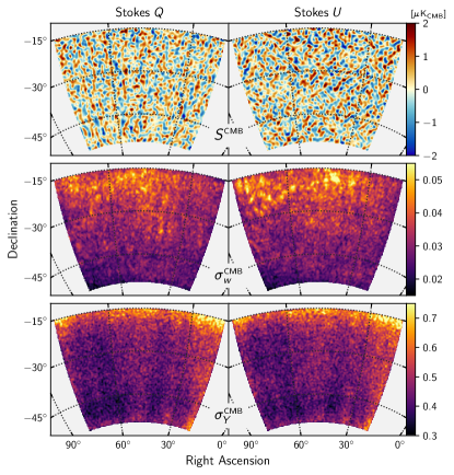
Figure 2: (top) SMICA derived component separated Stokes $Q$/$U$ CMB maps computed with the CMB weights shown in the left panels of Figure 1. (middle) The contribution $\sigma_{w}$ to the uncertainty in the CMB maps due to uncertainty in the SMICA weights. (bottom) The contribution $\sigma_{Y}$ to the CMB map uncertainty due to the uncertainty in the input Spider and Planck data maps. All maps are in units of $\mu$K_CMB.

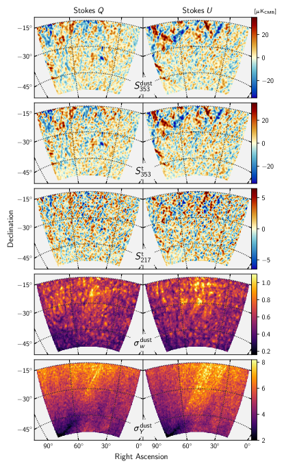
Figure 3: (row 1) SMICA derived component separated Stokes $Q$/$U$ dust maps, computed with the dust weights shown in the right panels of Figure 1, and scaled to the 353 GHz reference frequency. (rows 2 and 3) The 353 GHz and 217 GHz Planck map templates are reobserved and band-limited to $\ell\in[8,258]$. The SMICA dust map shows structure that is most consistent with the 353 GHz template, the predominant contribution to the component weights. (row 4) The contribution $\sigma_{w}$ to the uncertainty in the SMICA dust maps due to uncertainty in the weights. (row 5) The contribution $\sigma_{Y}$ to the dust map uncertainty due to the uncertainty in the input Spider and Planck data maps. Note that the morphology of $\sigma_{Y}$ is inconsistent with that of $\sigma_{w}$. All maps are in units of $\mu$K_CMB.

Figure 1 shows the weights by which each Spider and Planck HFI frequency map contribute to the component maps computed by SMICA. For the dust component, the relative contribution of the map at frequency $\nu$ is given by its SMICA ($a_{\ell m}$) weight multiplied by $f_{\nu}\equiv a_{\nu}^{\mathrm{dust}}$, the $\nu$-component of the vector $a^{\mathrm{dust}}$, the dust frequency scaling vector fitted to the data by SMICA. The main contributor to both the $E$-mode and $B$-mode dust signals in Figure 1 is the 353 GHz Planck map, which has the highest ratio of dust signal to noise. In the $B$-mode dust reconstruction, all contributions are positive, as expected in the absence of CMB $B$-mode power.

For the CMB, the SMICA weight for a given frequency map directly represents its relative contribution, since $a^{\mathrm{CMB}}$ is the identity vector. The Spider maps provide the dominant contribution to both the $E$ and $B$-modes, reflecting the higher ratios of CMB signal to noise in these maps than in any of the Planck HFI maps.

The $Q$ and $U$ maps derived by SMICA, along with their estimated uncertainties, are shown in Figures 2 and 3 for the CMB and dust components, respectively. The covariance $\sigma_{w}$ of the weights and the noise covariance $\sigma_{Y}$ contribute in quadrature to the total per-pixel uncertainty on the estimates of the component maps $S$. The former represents the uncertainty due to signal reconstruction, while the latter (the dominant term) represents the per-pixel noise after a weighted average. Both are presented in separate panels of Figures 2 and 3.

In Figure 3, the morphology of $\sigma_{Y}^{\textrm{dust}}$ is similar to noise estimates for Planck 353 GHz, as that map dominates the weight. The uncertainty on the dust reconstruction, $\sigma_{w}^{\textrm{dust}}$, is morphologically distinct from the noise. In particular, the larger uncertainty in the upper third of the $\sigma_{w}^{\textrm{dust}}$ maps does not trace the reconstructed dust signal strength or the noise. This unexpected structure could come from unidentified systematic errors in the input Planck or Spider maps, although evidence for the latter was not found in the expansive suite of null tests published in SPIDER Collaboration et al. (2022). A physical origin is also possible: frequency decorrelation, in which dust emission at a given frequency is not well correlated with that at other frequencies, would prevent an accurate reconstruction of this emission by SMICA, as the formalism here assumes that a single frequency scaling factor applies to all pixels. Given a specific frequency decorrelation model, e.g., a mixture of two dust populations, each characterized by its own spectral index, simulations could be run through SMICA in an attempt to reproduce the structure observed in the dust uncertainty maps. Such a study is beyond the scope of our analysis.

Figure 3 also compares the SMICA dust component map $S\mathrm{{}_{353}^{dust}}$ to the Planck dust template maps $S\mathrm{{}_{\nu_{0}}^{t}}$ constructed with $\nu_{0}=$ 353 GHz and $\nu_{0}=$ 217 GHz. The template maps have been band-limited to $\ell\in[8,258]$, to match the scales for which SMICA weights are fit. The $S\mathrm{{}_{353}^{dust}}$ and $S\mathrm{{}_{353}^{t}}$ maps look very similar, which is not surprising since both are dominated by Planck 353 GHz data. $S\mathrm{{}_{217}^{t}}$ has much lower dust amplitude than $S\mathrm{{}_{353}^{t}}$, and lower signal-to-noise ratio. The visible structures in these two template maps are similar but not identical.

3 Spatial Dependence of Polarized Dust Emission Properties

In our baseline cosmological analysis (SPIDER Collaboration et al., 2022), we use foreground-template subtraction (Section 2.1) to subtract the polarized emission from interstellar dust from the Spider maps. As reflected in the scalar nature of $A_{\nu,\nu_{0}}$ (and therefore of $\alpha$) in Equation 3, this procedure assumes that the morphology of this emission is independent of frequency. This assumption could easily be inadequate, e.g., if the temperature of dust grains changes across the Spider region, or if two or more dust populations—even if they are well mixed—permeate it. In Section 3.2, we perform foreground-template subtraction independently in two non-overlapping, physically motivated subregions of the Spider field (described in Section 3.1), and assess the consistency of the $\alpha$ values derived in the two subregions. We discuss the physical interpretation of these results in Section 3.3.

3.1 Delineating Subregions

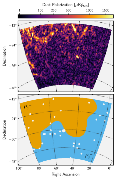
Figure 4: (top) The polarization $P^{2}=Q^{2}+U^{2}$ of the SMICA-derived dust component (first row of Figure 3). (bottom) Mask regions ${P_{\mathrm{d}}}^{+}$ and ${P_{\mathrm{d}}}^{-}$, containing more or less polarized dust, respectively, as inferred from the polarization map.

We define two physically motivated subregions within the Spider field based upon a SMICA-generated map of the total polarized dust emission power, $P^{2}=Q^{2}+U^{2}$ (Figure 4, top). This map is constructed from the $Q\mathrm{{}_{353}^{dust}}$ and $U\mathrm{{}_{353}^{dust}}$ Stokes parameter maps described in Section 2.2 and shown in Figure 3. After smoothing this map with a Gaussian of $8^{\circ}$ FWHM, we separate the map into two complementary subregions along the $P^{2}=100\,\mu\mathrm{K}_{\mathrm{CMB}}^{2}$ contour (Figure 4, bottom). We denote by ${P_{\mathrm{d}}}^{+}$ (${P_{\mathrm{d}}}^{-}$) the subregion in which $P^{2}$ is greater (less) than this threshold. This procedure produces two simply-connected subregions (prior to masking point sources) that are separated by a smooth boundary, features that facilitate power spectrum estimation (Gambrel et al., 2021). After point-source masking according to the procedure described in SPIDER Collaboration et al. (2022), ${P_{\mathrm{d}}}^{+}$ and ${P_{\mathrm{d}}}^{-}$ cover roughly equal sky fractions of 2.4% and 2.3%, respectively. We note in passing that ${P_{\mathrm{d}}}^{-}$ overlaps with the “Southern Hole,” a region of the Southern sky that has long been known to exhibit low total dust emission, and that has more recently been mapped with high polarization sensitivity (BICEP/Keck Collaboration et al., 2021; Balkenhol et al., 2023).

3.2 Template Subtraction by Subregion: Evidence for Spatial Variation

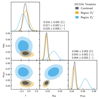
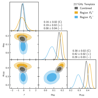
Figure 5: The XFaster likelihood contours for $r$, $\alpha_{95}$, and $\alpha_{150}$ with the combined Spider region in gray and ${P_{\mathrm{d}}}^{+}$ and ${P_{\mathrm{d}}}^{-}$ subregions in orange and light blue, respectively, computed independently with the 353 GHz dust template (left) and the 217 GHz dust template (right). Central values and $1\,\sigma$ errors for each of the three regions are indicated in the titles for the $\alpha$ parameters.

Following the procedure described in Section 2.1, we perform foreground template subtraction independently on each of the two subregions defined in Section 3.1. The left panel of Figure 5 shows, for each subregion and for the entire Spider field, the resulting 1-D and 2-D likelihoods for the tensor-to-scalar ratio, $r$, and for the foreground-template fitting parameters, $\alpha_{95}$ and $\alpha_{150}$, where the added indices refer to the Spider frequencies to which we fit the Planck 353 GHz foreground template. Following the method in Section 4.3 of Gambrel et al. (2021), the results in this section are validated with a suite of 300 simulations with input $r$, $\alpha_{95}$, and $\alpha_{150}$ fixed to the maximum likelihood values in Figure 5. Each simulated map is constructed from ensembles of CMB plus Spider noise, along with either the 217 or 353 GHz Planck dust template. Fitted templates add noise from Planck FFP10 realizations. To produce robust estimates of the $\alpha$ parameters recovered from the Spider data, we correct the data likelihoods for a small ($\ll 1\,\sigma$) bias in the XFaster estimator, as measured from this validation suite.

With the Planck 353 GHz template, we find the maximum-likelihood values for $r$ and $\alpha_{95}$ to be consistent to better than $0.7\,\sigma$ and $2.0\,\sigma$, respectively, between all three regions. However, the maximum-likelihood values for $\alpha_{150}$ differ by $3.6\,\sigma$ between the two subregions, with a significantly higher value of $\alpha_{150}$ in ${P_{\mathrm{d}}}^{-}$ than in ${P_{\mathrm{d}}}^{+}$. In other words, the template-correlated dust signal in the more diffuse region, ${P_{\mathrm{d}}}^{-}$, is brighter than would be inferred by scaling the template based upon observations of the region with more polarized dust emission, ${P_{\mathrm{d}}}^{+}$ (or of the combined region, where the fit is naturally driven by the brighter areas). We would thus expect residual dust signal after subtraction of a template that did not account for such variability.

Note that these data are not sufficient to establish any general causal relationship between variation in $\alpha_{150}$ and the intensity of the dust $P$ map. This would require comparisons between a larger number of subregions, which is beyond the scope of this work.

We are able to reject a number of compact structures as the origin of this discrepancy. Two regions of particular interest are the Orion-Eridanus Superbubble (Finkbeiner, 2003; Soler et al., 2018) and the Magellanic Stream (Mathewson et al., 1974). The former, which features prominently in H$\alpha$ maps, occupies about 20% of the full Spider region, mostly located in ${P_{\mathrm{d}}}^{+}$. Although the Magellanic Stream falls mostly outside the Spider region, some high-velocity clouds have been mapped on the outskirts of its bottom-right corner (HI4PI Collaboration et al., 2016). Even though we do not necessarily expect the dust emission from these regions to dominate the polarized emission in our maps, high levels of polarization along the edge of the Orion-Eridanus Superbubble and hints of variation in dust properties between the Galaxy and the Magellanic Clouds (Galliano et al., 2018) warrant caution. As documented in Appendix A, we find the measured spatial variation in $\alpha_{150}$ to be robust to masking aimed at probing the impact of these structures.

We further explore the discrepancy in $\alpha$ between subregions by repeating this template subtraction analysis with an alternate dust template, constructed by substituting the 217 GHz Planck map for the 353 GHz map. The 217  GHz data also contain substantial polarized dust emission, as evidenced by the fact that they provide the second-largest contribution to the SMICA dust reconstruction (Figure 1). The right panel of Figure 5 shows the 1-D and 2-D likelihoods for $r$, $\alpha_{95}$, and $\alpha_{150}$ in this configuration. We again find $r$ to be consistent (within $0.2\,\sigma$) between the two subregions, a moderate discrepancy in $\alpha_{95}$ ($2.7\,\sigma$), and a larger discrepancy in $\alpha_{150}$ ($3.5\,\sigma$). However, while the latter discrepancy has similar significance to that found with the 353 GHz template, it is in the opposite direction: $\alpha_{150}$ is found to be lower in ${P_{\mathrm{d}}}^{-}$ than in ${P_{\mathrm{d}}}^{+}$.

3.3 Implications for a Modified-Blackbody Model

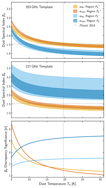
Figure 6: $1\,\sigma$ contours of possible $T_{\mathrm{d}}$ and $\beta_{\mathrm{d}}$ for the $\alpha$ values found with the XFaster framework and presented in Figure 5. (top) Using the 353 GHz dust template, the ${P_{\mathrm{d}}}^{+}$ region is identified with a higher $\beta_{\mathrm{d}}$ or a higher $T_{\mathrm{d}}$, while the ${P_{\mathrm{d}}}^{-}$ region is identified with a lower $\beta_{\mathrm{d}}$ or $T_{\mathrm{d}}$. (middle) With the 217 GHz template, the ${P_{\mathrm{d}}}^{+}$ region is instead identified with a lower $\beta_{\mathrm{d}}$ or $T_{\mathrm{d}}$ than the ${P_{\mathrm{d}}}^{-}$ region. (bottom) Mutual significance of the discrepancy in $\beta_{\mathrm{d}}$ between the two templates, as a function of assumed $T_{\mathrm{d}}$. The $\beta_{\mathrm{d}}$ values found in the ${P_{\mathrm{d}}}^{-}$ region are discrepant at $>3\,\sigma$, while the significance of the discrepancy is $<2\,\sigma$ in the ${P_{\mathrm{d}}}^{+}$ region. The Planck 2018 all-sky best fit parameters ($\beta_{\mathrm{d}}=1.53$, $T_{\mathrm{d}}=19.6$ K) are also shown for reference (dotted lines).

In the context of the simple MBB model of Equation 1, the template scaling parameter $\alpha$ is a function of the dust model parameters—the dust temperature, $T_{\mathrm{d}}$, and the spectral index of polarized emission, $\beta_{\mathrm{d}}$—as well as the frequencies of the maps used to build the dust template and the frequency of the map to which the template is fitted. Specifically,

$$A_{\nu,\nu_{0}}=\frac{(e^{\,x}-1)^{2}}{x^{2}e^{\,x}}\frac{{x_{0}}^{2}e^{\,x_{0}}}{(e^{\,x_{0}}-1)^{2}}\left(\frac{\nu_{0}}{\nu}\right)^{\!2}\left(\frac{\nu^{\mathrm{d}}}{\nu_{0}^{\mathrm{d}}}\right)^{\!\beta_{\mathrm{d}}}\frac{B(\nu^{\mathrm{d}},T_{\mathrm{d}})}{B(\nu^{\mathrm{d}}_{0},T_{\mathrm{d}})},$$ (5)

where the superscript “d” added to the frequency of a map indicates that its effective band center is computed for a dust SED instead of the CMB SED, as discussed in Appendix B, and we have used the shorthand $x\equiv h\nu/(kT_{\mathrm{CMB}})$.

Using this relationship, we can translate the 1-D likelihoods for $\alpha_{95}$ and $\alpha_{150}$ shown in Figure 5 into contour plots in $(T_{\mathrm{d}},\beta_{\mathrm{d}})$. The results are shown in Figure 6. These parameter constraints allow us to perform several internal comparisons within the MBB model context, which are discussed in the paragraphs below.

Comparing Spider frequencies

The $\beta_{\mathrm{d}}$ values inferred from the fitted $\alpha_{95}$ and $\alpha_{150}$ show excellent consistency (${<}1\,\sigma$) with one another for either choice of dust template, except perhaps in ${P_{\mathrm{d}}}^{+}$ at the very lowest dust temperatures ($T_{\mathrm{d}}\lesssim 7\,\mathrm{K}$). In other words, if we confine ourselves to a single Planck-derived dust template, the Spider data provide no significant evidence of deviation from an MBB SED in either subregion.

Comparing subregions

The values of $\alpha_{150}$ obtained using the $\nu_{0}=$ 353 GHz dust template translate into lower values of $\beta_{\mathrm{d}}$ in ${P_{\mathrm{d}}}^{-}$ compared to ${P_{\mathrm{d}}}^{+}$ for any value of $T_{\mathrm{d}}$. Specifically, if we fix $T_{\mathrm{d}}=19.6\,\mathrm{K}$ (Planck Collaboration et al., 2020b) throughout, we find $\beta_{\mathrm{d}}=1.52\pm 0.06$ in ${P_{\mathrm{d}}}^{+}$ and $1.09\pm 0.09$ in ${P_{\mathrm{d}}}^{-}$. Importantly, the value of $\beta_{\mathrm{d}}$ inferred independently from $\alpha_{95}$ is consistent with that of $\alpha_{150}$, with comparable significance. Taken at face value, this $3.9\,\sigma$ inconsistency in $\beta_{\mathrm{d}}$ would indicate a spatial variation in dust composition between the ${P_{\mathrm{d}}}^{+}$ and ${P_{\mathrm{d}}}^{-}$ subregions.

If we instead fix the dust spectral index to be $\beta_{\mathrm{d}}=1.53$ (Planck Collaboration et al., 2020b) in both subregions, we find a large difference in implied dust temperatures: $T_{\mathrm{d}}=19.1^{+3.7}_{-2.5}\,\mathrm{K}$ in ${P_{\mathrm{d}}}^{+}$, $T_{\mathrm{d}}=9.2^{+1.1}_{-0.8}\,\mathrm{K}$ in ${P_{\mathrm{d}}}^{-}$. Although we certainly expect some lack of uniformity in dust temperature—stemming from spatial variation in the dust’s radiative environment—such a large variation in the temperature of the diffuse interstellar medium at high Galactic latitude may be unphysical given our current understanding of dust physics (Li & Draine, 2001; Draine & Li, 2007).

A similar discrepancy between subregions (though of opposite sign) is visible with the 217 GHz dust template, as shown in the middle panel of Figure 6. Fixing $T_{\mathrm{d}}=19.6\,\mathrm{K}$ with the $\alpha_{150}$ constraint results in $\beta_{\mathrm{d}}=1.37\pm 0.08$ in ${P_{\mathrm{d}}}^{+}$ and $2.1^{+0.3}_{-0.2}$ in ${P_{\mathrm{d}}}^{-}$, a $3.2\,\sigma$ discrepancy. Alternatively, fixing $\beta_{\mathrm{d}}=1.53$ gives $T_{\mathrm{d}}=12^{+3}_{-2}\,\mathrm{K}$ for ${P_{\mathrm{d}}}^{+}$, but no value of $T_{d}$ accommodates $\beta_{\mathrm{d}}=1.53$ within ${P_{\mathrm{d}}}^{-}$.

Comparing dust templates within ${P_{\mathrm{d}}}^{-}$

The values of $\beta_{\mathrm{d}}$ derived from $\alpha_{150}$ within the ${P_{\mathrm{d}}}^{-}$ subregion using the $\nu_{0}=217$ GHz dust template are inconsistent with those derived using the $\nu_{0}=353$ GHz template. The bottom panel of Figure 6 shows the significance of this discrepancy as a function of dust temperature: it exceeds $3\,\sigma$ ($4\,\sigma$) for any $T_{\mathrm{d}}\gtrsim 5\,\mathrm{K}$ ($T_{\mathrm{d}}\gtrsim 15\,\mathrm{K}$). Under the assumption that the morphology of the polarized emission from interstellar dust is identical in both templates, this result corresponds to a statistically significant break in $\beta_{\mathrm{d}}$ for any physical $T_{\mathrm{d}}$, with the index having a lower value at the higher frequency.

Furthermore, we find that the value of $\alpha_{150}$ increases from ${P_{\mathrm{d}}}^{+}$ to ${P_{\mathrm{d}}}^{-}$ with the $\nu_{0}=353$ GHz template, but decreases from ${P_{\mathrm{d}}}^{+}$ to ${P_{\mathrm{d}}}^{-}$ with the $\nu_{0}=217$ GHz template. This observation is difficult to interpret under the assumption that the morphology of the polarized emission from interstellar dust is identical in both templates. This can be reconciled by assuming the existence of more than one dust population (which may be inferred from the spatial variation in $\beta_{\mathrm{d}}$ detected with the $\nu_{0}=353$ GHz template) combined with a break in $\beta_{\mathrm{d}}$ between 217 and 353 GHz.

Discussion

The physical interpretation in this section of the results derived in Section 3.2 points to a more complex picture of the polarized emission from interstellar dust in the Spider region than that provided by a single-component MBB model.

Taking the observations above together, we conclude: i) Unless $T_{\mathrm{d}}$ exhibits large variations at high Galactic latitudes, the spatial variation in $\alpha$ between ${P_{\mathrm{d}}}^{+}$ and ${P_{\mathrm{d}}}^{-}$ may be evidence of multiple dust populations (i.e., differing compositions, and thus emissivities); ii) Unless the $\nu_{0}=217$ GHz dust template is morphologically inconsistent with the $\nu_{0}=353$ GHz template, the inconsistency between the value of $\alpha$ derived in ${P_{\mathrm{d}}}^{-}$ with one template and that found in the same subregion with the other template would indicate a break in the value of $\beta_{\mathrm{d}}$ between 217 and 353 GHz; iii) The break in $\beta_{\mathrm{d}}$ may itself be composition dependent in order to simultaneously explain the increase in $\alpha$ between ${P_{\mathrm{d}}}^{+}$ and ${P_{\mathrm{d}}}^{-}$ observed with the $\nu_{0}=353$ GHz template and its decrease obtained with the $\nu_{0}=217$ GHz template. If this rather complex picture holds as more data (such as the Spider 280 GHz maps) become available, it may provide new insights into the properties of the interstellar medium, and associated modeling uncertainties would need to be taken into account in upcoming searches for cosmological $B$-modes.

4 Testing Standard Dust Modeling

The SMICA framework offers a high degree of flexibility in modeling the characteristics of dust. The SMICA pipeline implemented for the analysis in SPIDER Collaboration et al. (2022) incorporates a MBB model for the dust foreground component with the following characteristics:

• A single $\beta_{\mathrm{d}}$ parameter that is common across all multipoles and polarizations,

• A dust amplitude $A_{\mathrm{d}}$ that is free to vary across multipoles and polarizations,

• A $\delta$-function prior of $T_{\mathrm{d}}=19.6\,\textrm{K}$ to fix the dust temperature at the Planck all-sky value, and

• A Gaussian prior on $\beta_{\mathrm{d}}$ centered at the Planck all-sky value $\beta_{\mathrm{d}}=1.53$, with a generous width of $\sigma_{\beta_{\mathrm{d}}}=1.5$.

In this section, we quantify how these foreground modeling choices impact the best-fit CMB and foreground parameters recovered with the combined Spider and Planck data. Throughout this section, we leave the dust temperature fixed, due to a lack of sufficient constraining power and frequency coverage to simultaneously estimate both $\beta_{\mathrm{d}}$ and $T_{\mathrm{d}}$, while varying the constraints on $A_{\mathrm{d}}$ and/or $\beta_{\mathrm{d}}$. Here, unlike the discussion in Section 3.3, we apply the analysis to the full Spider region. The results in this section are therefore driven by the higher signal-to-noise component, corresponding approximately to the ${P_{\mathrm{d}}}^{+}$ contours of Figure 6.

4.1 SED Modeling of Polarized Dust Emission

Table 1: The best-fit dust amplitude $A_{\mathrm{d}}$ for each of the input frequency maps relative to that of the Planck 353 GHz map. The values tabulated here are also plotted in Figure 7. Best-fit values are computed as the median of the posterior distribution, with $1\,\sigma$ errors determined from the 68% interval on either side of the median.

		Dust Amplitude
Instrument	Band	EE			BB
Spider	95 GHz	$0.019$	$\pm$	$0.005$	$0.016$	${}_{-}^{+}$	${}_{0.004}^{0.005}$
	150 GHz	$0.047$	${}_{-}^{+}$	${}_{0.004}^{0.005}$	$0.047$	$\pm$	$0.003$
Planck	100 GHz	$0.018$	${}_{-}^{+}$	${}_{0.006}^{0.005}$	$0.028$	$\pm$	$0.007$
	143 GHz	$0.043$	$\pm$	$0.008$	$0.039$	$\pm$	$0.010$
	217 GHz	$0.139$	$\pm$	$0.013$	$0.123$	$\pm$	$0.014$

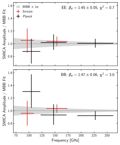
Figure 7: Testing the fidelity of the MBB dust model in the Spider high-latitude region for $E$- (top) and $B$- (bottom) modes. All data are plotted relative to the best-fit MBB model for that polarization component (gray band indicates the $1\,\sigma$ fit envelope), and account for the detector bandpass at each frequency. The horizontal error bars indicate the effective detector bandwidth over which the amplitudes are computed. The SMICA best-fit dust amplitudes ($+$) are consistent with the best-fit MBB model. The Spider data (red) have smaller error bars on $A_{\mathrm{d}}$, and therefore more constraining power, than the Planck data (black) in nearby bands.

We begin by testing the SED model of dust emission by fitting an independent amplitude $A_{\mathrm{d}}$ at each frequency, operating under the assumption that this amplitude remains consistent across multipoles. As discussed in SPIDER Collaboration et al. (2022), dust and noise exhibit similar scaling behaviors with frequency, making it challenging for an ICA-based algorithm to distinguish between the two components. By relaxing the prior constraint on $\beta_{\mathrm{d}}$ and fitting for the dust amplitudes directly, we are able to circumvent this noise/dust scaling degeneracy. The resulting amplitudes can then be fit to a MBB model to recover the best-fit $\beta_{\mathrm{d}}$ value.

The dust amplitudes recovered with this algorithm are listed in Table 1 for each of the Spider and Planck frequency bands, and the resulting MBB model fit is illustrated in Figure 7. Fitting a spectral index to each set of six frequency maps results in a best-fit value of $\beta_{\mathrm{d}}$ of $1.45\pm 0.05$ ($1.47\pm 0.06$) for the $EE$ ($BB$) components, with $\chi^{2}$ values of 0.7 (3.0), respectively. With approximately four degrees of freedom, these $\chi^{2}$ values indicate that a single-component MBB model is an adequate description of the Spider + Planck dataset, thus justifying the use of the MBB model for constraining foreground power in the CMB $B$-mode analysis. Additionally, Figure 7 illustrates the improved constraining power of the Spider data at 95 and 150 GHz in this region of the sky relative to that of the nearby Planck bands at 100 and 143 GHz.

4.2 Angular Scale Dependence of Dust Spectral Index

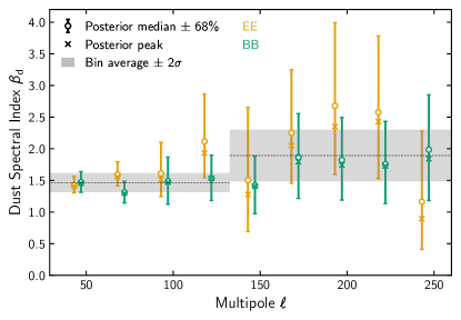
Figure 8: An analysis of the variation of the dust spectral index over angular scale using the SMICA pipeline. Each point covers a binned multipole range of $\Delta\ell=25$, with $E$ and $B$ points offset in $\ell$ for clarity. The distributions of the best fit $\beta_{\mathrm{d}}$ in each bin are not Gaussian; the median ($\circ$) and peak ($\times$) of each posterior are indicated. The error bars correspond to 68% intervals on either side of the median, equivalent to 1 $\sigma$ for a non-Gaussian distribution. The best-fit $\beta_{\mathrm{d}}$ values agree to within a mutual $2\,\sigma$ between the larger and smaller angular scales. The $E$ and $B$ $\beta_{\mathrm{d}}$ values are statistically consistent with each other at all scales.

Next we test the assumption of a scale-independent SED by fitting the MBB model independently for each polarization as a function of $\ell$. The results of this fit for $\beta_{\mathrm{d}}$ are shown in Figure 8. The best-fit spectral index values agree to within $\sim 0.5\,\sigma$ between the $E$ and $B$ polarization components across all angular scales, providing no evidence for including a polarization-dependence in the model. Comparing the best-fit $\beta_{\mathrm{d}}$ values averaged over larger ($\ell<140$) and smaller ($\ell>140$) angular scales shows agreement to within $2\,\sigma$.

When analyzed over the full Spider region, the data do not reveal any strong evidence of variations in spectral index with polarization mode or angular scale, further justifying the adoption of the simple MBB dust model.

4.3 Angular Scale Dependence of Dust Amplitude

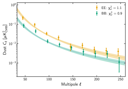
Figure 9: A power-law model fit to the SMICA-derived dust amplitudes as a function of angular scale. The best-fit model, shown as a band indicating the $1\,\sigma$ error on the fit, is binned identically to the SMICA-derived dust bandpowers in order to compute the $\chi^{2}$ of the fit. The reported $\chi^{2}_{\nu}$ values are computed using the full covariance of both the power-law model and the SMICA bandpowers, and assume seven degrees of freedom. The best-fit model parameters are shown in Figure 10.

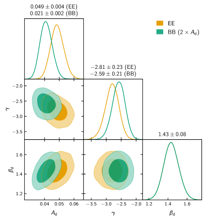
Figure 10: The covariance of the fitted dust parameters for the model shown in Figure 9. Central values with $1\,\sigma$ errors are indicated in the titles for each of the three parameters. The best-fit $A_{\mathrm{d}}$ and $\sigma_{A_{\mathrm{d}}}$ for the $BB$ component is scaled by a factor of 2 for better visual comparison to its $EE$ counterpart, with its true central value indicated in the column title.

Dust emission is often (e.g., Planck Collaboration et al. (2020b); BICEP/Keck Collaboration et al. (2021)) modeled as a power law in $C_{\ell}$:

$$C_{\ell}=A_{\mathrm{d}}(\nu)\left(\frac{\ell}{80}\right)^{\gamma}.$$ (6)

We can fit this model to the SMICA-derived amplitudes as a function of $\ell$-bin independently for the $E$ and $B$ polarization components. We assume a single-component MBB scaling of the amplitude with frequency, common to both polarizations. The results of this fit are shown in Figures 9 and 10, with reduced $\chi_{\nu}^{2}=1.1(0.9)$ for the $E$ ($B$) polarization components, assuming $\nu=7$. This analysis finds a dust spectrum that falls steeply, $\gamma^{EE}=-2.81\pm 0.23$, with no significant difference in best-fit values between the two polarizations. We note that Planck has reported values of $-2.42$ and $-2.54\pm 0.02$ in the largest area of sky for $EE$ and $BB$, respectively. In the most restrictive mask, Planck finds more shallow indices of $-2.28\pm 0.08$ and $-2.16\pm 0.11$ for $EE$ and $BB$ (Planck Collaboration et al., 2020b).

The Spider dataset also provides an additional observational constraint on the asymmetry in dust power between $EE$ and $BB$ polarization modes, visible in Figure 10. This analysis finds an $EE/BB$ dust power ratio of $2.1\pm 0.3$ at large scales ($\ell<140$). This result aligns with prior findings from Planck (Planck Collaboration et al., 2016a). The origin of this dust power asymmetry is not conclusively understood. Some studies investigate the role of magnetohydrodynamic (MHD) turbulence in the interstellar medium (ISM) (Caldwell et al., 2017; Kandel et al., 2017), while others suggest that this power asymmetry can be a probe of the dust filament aspect ratio (Huffenberger et al., 2020) and magnetic field alignment (Clark et al., 2021).

4.4 Impact on Cosmological $B$-mode Measurements

At the level of sensitivity of contemporary observational programs, the contribution of modeling uncertainty to limits on the cosmological CMB $B$-mode signal is non negligible even in those regions of the sky with low levels of Galactic emission. In this section we attempt to quantify the impact of these complexities on the uncertainty in the tensor-to-scalar ratio, $\sigma_{r}$, within the Spider region.

Following the analysis in SPIDER Collaboration et al. (2022), for each dust model we can compute the $\sigma_{r}$ derived from an ensemble of sky and noise simulations constructed to match the model under consideration. In the configuration where there is no SED modeling and SMICA fits a dust amplitude per frequency, we find $\sigma_{r}=0.130$. If instead a spectral index $\beta_{\mathrm{d}}$ is fit per multipole, allowing for dust behavior to change with scale, we find $\sigma_{r}=0.128$. Constraining the spectral index to a single value over all scales, as in SPIDER Collaboration et al. (2022), we find $\sigma_{r}=0.116$. Finally, the assumption that dust follows a power-law in multipole space does not improve $\sigma_{r}$ further. We find instead that this assumption re-distributes the uncertainties: the uncertainty near the pivot scale ($\ell\sim 80$) is reduced, while that at larger scales increases. Thus, we find that the complexities in foreground modeling described in this section can contribute at the level of $\sigma_{r}\sim 0.012$, corresponding to a ${\sim}10\%$ impact on $\sigma_{r}$ in the case of Spider.

4.5 Discussion

When applied to the full area of sky observed by the Spider experiment, the variations of the nominal SMICA algorithm described above, each employing different assumptions about foreground modeling, all point to a consistent description of polarized Galactic dust emission. These data are consistent with dust characterized by a single-component, modified black-body model across the Spider and Planck frequencies and for both polarization parity modes. The dependence on angular scale is consistent with an approximate power-law dependence on multipole, $\ell$. The combined Spider and Planck data over this restricted region prefer a dust emissivity spectral index $\beta_{\mathrm{d}}=1.45\pm 0.07$, somewhat lower than the all-sky Planck 2018 value (Planck Collaboration et al., 2020b) of $\beta_{\mathrm{d}}=1.53\pm 0.02$ with $T_{\mathrm{d}}=19.6K$. The foreground complexities considered in this section are found to contribute to the uncertainty on the tensor-to-scalar ratio at the level of $\sigma_{r}\sim 0.012$.

5 Line-of-sight Decorrelation of Dust

In addition to the search for spatial variation in Section 3, we use Spider data to perform a search for variation in the polarization angle of dust emission with frequency. Such a rotation with frequency may indicate the presence of multiple dust clouds along a line of sight with different SEDs and magnetic alignments. For example, (Pelgrims et al., 2021) used HI line emission maps to identify regions of the sky likely to contain magnetically-misaligned clouds; they compute the difference in polarized dust angle for these different populations to demonstrate that LOS frequency decorrelation is detectable within the Planck dataset, largely in the Northern Galactic cap. An analysis by the BICEP team (BICEP/Keck Collaboration et al., 2023) showed no evidence of dust decorrelation within their observation region.

We perform this search by constructing a set of dust templates as in Section 2.1, each derived from a single Spider or Planck map. In this case, we opted to subtract CMB signal using the SMICA-derived CMB template rather than the Planck 100 GHz map, due to its lower overall noise level. From each template, we compute a map of polarized dust angle using the unbiased estimator (Plaszczynski et al., 2014)

$$\psi=\frac{1}{2}\arctan(U,Q).$$ (7)

We construct a likelihood estimator to evaluate the consistency of the measured dust angle $\psi$ at different frequencies.

In order to construct our likelihood, we approximate the uncertainty on $\psi$ as Gaussian. We estimate this uncertainty with standard error propagation:

$$\sigma_{\psi}^{2}=\frac{1}{4}\frac{Q^{2}\sigma_{U}^{2}+U^{2}\sigma_{Q}^{2}}{(Q^{2}+U^{2})^{2}}\\ +\frac{Q^{2}U^{2}}{2(Q^{2}+U^{2})^{4}}\left[\sigma_{Q}^{4}+\sigma_{U}^{4}+\frac{1}{2}\frac{(Q^{2}-U^{2})^{2}}{Q^{2}U^{2}}\sigma_{Q}^{2}\sigma_{U}^{2}\right]$$ (8)

where the two grouped terms represent the first- and second-order errors respectively. We expect these uncertainties to be underestimated when the signal-to-noise is low ($\sigma_{U}^{2}+\sigma_{Q}^{2}>U^{2}+Q^{2}$). However, the Gaussian approximation breaks down as higher-order terms become more significant. To address this, we apply a mask to reject map pixels for which the second-order errors on polarized dust angle exceed the first. This criterion rejects 20-30% of the sky area covered by the Spider instrument. This thresholding serves two main purposes: (1) to exclude pixels whose uncertainties are challenging to model accurately, and (2) to remove pixels with especially large uncertainties, for which the width of the distribution would wrap around the range of the arctangent function, yielding non-Gaussian behavior. While the statistical properties of $\psi$ are complex and cannot be strictly Gaussian, the Gaussian distribution serves as a reasonable approximation after this thresholding.

From a given pair of dust maps $X$ and $Y$ we calculate a pair of dust angles ($\psi^{X}_{i},\psi^{Y}_{i}$) for each map pixel $i$. To this we fit a Gaussian mixture model (Hogg et al., 2010) in which each pixel can belong to one of two populations: a base population, for which the dust angle is consistent between our pair of maps up to some constant angular offset $\Delta\psi$; and a second population of outlier pixels, for which the polarization angle is inconsistent between the two frequencies. The first population probes a possible systematic offset in polarization angle between maps at different frequencies; this is expected to be consistent with zero, and unlikely to arise from dust decorrelation given the relatively large sky area covered by Spider. The second population is our probe of decorrelated dust, in the form of isolated, dense cloud structures with arbitrary polarization angles relative to our line of sight.

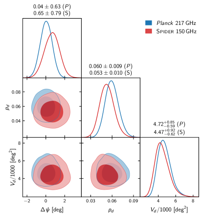
Figure 11: Best-fit model parameters for the dust angle decorrelation likelihood defined in Equation 9: global dust angle offset $\Delta\psi$ in degrees, population fraction $p_{d}$ of pixels with measurable angle differences, and additional variance $V_{d}$ in square degrees introduced by these outlier pixels. We find that $\Delta\psi$ is statistically consistent with zero, indicating that the dust angle appears globally consistent between the Planck 353 GHz frequency map and lower frequencies Planck 217 GHz (blue) and Spider 150 GHz (red). The likelihoods are marginalized over $\{q_{i}\}$, and central values with $1\,\sigma$ errors are indicated in the titles.

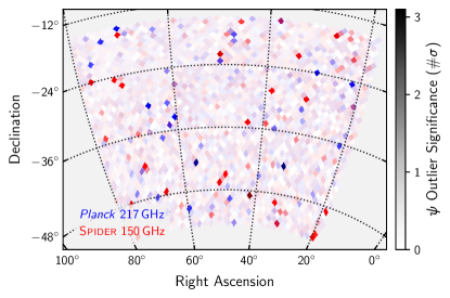
Figure 12: The significance in $\sigma$ of the probability $p_{i}$ that the measured dust angle in each map pixel $i$ is inconsistent between the Planck 353 GHz map and either the Planck 217 GHz map (blue) or the Spider 150 GHz map (red). The significance is encoded such that bright purple pixels are likely in the outlier population in both frequency pair analyses. The lack of both astrophysical structure and overlap between the two populations argues against local decorrelation in the Spider observing region.

Our likelihood takes the form

$$\mathcal{L}(\{q_{i}\},\Delta\psi,p_{d},V_{d})=\\ \prod_{i}\left[\frac{1}{\sqrt{2\pi\Sigma_{i}}}\exp\left(-\frac{\Delta_{i}^{2}}{2\Sigma_{i}}\right)\right]^{1-q_{i}}\times\\ \left[\frac{1}{\sqrt{2\pi(\Sigma_{i}+V_{d})}}\exp\left(-\frac{\left(\psi^{X}_{i}\right)^{2}+\left(\psi^{Y}_{i}\right)^{2}}{2(\Sigma_{i}+V_{d})}\right)\right]^{q_{i}},$$ (9)

where

$$\Delta_{i} =\min_{\delta_{\pi}}\left\{\frac{1}{\sqrt{2}}\left((\psi^{Y}_{i}+\delta_{\pi})-(\psi^{X}_{i}+\Delta\psi)\right)\right\}$$ (10)

$$\Sigma_{i} =\frac{1}{2}\left(\sigma_{X}^{2}+\sigma_{Y}^{2}\right)$$ (11)

$$q_{i} \sim\text{BetaBinomial}\left(\alpha=p_{d},\beta=1-p_{d}\right)$$ (12)

The boolean $q_{i}$ assigns each pixel $i$ to one of the two populations. The generative model of the base population ($q_{i}=0$) is taken to be a two-dimensional Gaussian, with an orthogonal distance $\Delta_{i}$ between the two map angles for each pixel (Equation 10) and variance $\Sigma_{i}$ (the projected variance of the uncertainty of the pixel onto a line of slope of unity). Note that, because the domain of angles lies in the range $[-\pi/2,\pi/2]$, differences in $\psi$ by any multiple of $\pi$ are inconsequential. We account for this by minimizing over a nuisance parameter $\delta_{\pi}\in\{-\pi,0,\pi\}$ in Equation 10.

The second population represents outlier, or rejected, pixels, which show local differences in angle between the maps. We do not a priori have an expectation for the statistics of this population. We choose to model it as a two-dimensional Gaussian with zero mean and an additional variance $V_{d}$ (in excess of $\Sigma_{i}$).

Finally, we treat the pixel assignments $q_{i}$ probabilistically, such that each pixel has a probability $p_{i}$ of being assigned to the base population. The probability $p_{i}$ is itself drawn from a beta distribution with $\alpha=p_{d},\beta=1-p_{d}$, such that the expectation value $E(p_{i})=p_{d}$. In this way, $p_{d}$ can be thought of as a global parameter for the fraction of outlier pixels in the total population. All together, our model has $N_{\mathrm{pix}}+3$ variables: $N_{\mathrm{pix}}$ population assignments $q_{i}$, a systematic offset parameter $\Delta\psi$, and two parameters describing the variance ($V_{d}$) and population fraction ($p_{d}$) of the outliers.

We conduct two iterations of this analysis using pairs of maps with the highest signal-to-noise ratios for dust: one comparing the Planck 353 GHz and Spider 150 GHz maps, the other comparing Planck 353 GHz to Planck 217 GHz. Figure 11 shows the resulting uncertainties and covariances between the fit parameters $(\Delta\psi,p_{d},V_{d})$. Both comparisons find angular offsets $\Delta\psi$ consistent with zero to within $1\,\sigma$, with $p$-values of 0.21 (0.47) for $\Delta\psi_{150}$ ($\Delta\psi_{217}$). This suggests that the mean polarized dust angle at 353 GHz is consistent with those at lower frequencies.

Only about 5% of the pixels included in our analysis region are rejected and assigned to the outlier population. These pixels display discrepancies in dust angle between 353 GHz and the corresponding lower frequency. While these outliers could signify spatially-dependent decorrelation, a map of the locations of these pixels (Figure 12) reveals two key observations: (1) the regions lack the connectivity we might expect from a real astrophysical population, and (2) the outliers identified by the two analyses share little overlap. Indeed, only about 0.2% of pixels are identified as deviant in both analyses. This argues against interpreting these pixels as a detection of LOS decorrelation.

We can further perform a hypothesis test to estimate the probability of this analysis yielding 5% decorrelated pixels under the null hypothesis that there is no decorrelated dust at any frequency for the entire observed region. We construct a dust map from 353-100 GHz difference maps, then scale this to both 150 GHz and 217 GHz using a standard modified black-body dust model. To this we add realistic noise by drawing from an ensemble of simulations, specifically Spider noise simulations at 150 GHz and Planck FFP10 realizations at 217 GHz and 353 GHz. From these simulated dust + noise maps, we compute the dust angles and perform an identical analysis. Comparing our measurement of the fraction of outlier pixels, $p_{d}$, to this ensemble of simulations, we obtain $p$-values of 0.18 and 0.10, respectively, for the 150 GHz and 217 GHz analysis. We thus conclude that the inferred fraction of decorrelated pixels can be readily attributed to noisy measurements of Stokes $Q$ and $U$. Consequently, our analysis finds no evidence for LOS decorrelation in the Spider observing region. The dust angles at 353 GHz largely agree with those at the lower frequencies, and those pixels that show outsized deviations are plausibly caused by noise.

6 Comparison to PySM Dust Models

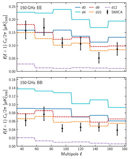
Figure 13: Comparison of the $EE$ (top) and $BB$ (bottom) spectra from several PySM3 dust models (colored lines) to SMICA-derived dust bandpowers at 150 GHz (black points) in the Spider region. Models based on the same underlying inputs and approach to SED modeling are shown with the same line style.

The SMICA dust maps derived from the combination of Spider and Planck data (shown in Figure 3) can also be used to test full-sky dust models. The Python Sky Model, commonly known as PySM, is a Python package designed for generating full-sky simulations of Galactic microwave foregrounds (Thorne et al., 2017). It is often used by the CMB community to test component separation methods and perform sensitivity forecasts. The current release, PySM3, contains thirteen distinct dust models that vary the assumptions and data processing of the underlying Planck data, allowing the user to generate full-sky dust emission maps at any frequency bandpass of interest.

To test the agreement between each of these models and our SMICA dust polarization maps, we first use PySM to generate maps in the Spider observing region using the measured 150 GHz frequency bandpass. We then compute binned $EE$ and $BB$ spectra for each PySM model using PolSPICE (Chon et al., 2004) and compare these to analogous spectra generated from the Spider-Planck SMICA dust maps described in Section 2.2.

Figure 13 shows these spectra for a representative subset of dust models, which were chosen to span the range of predicted dust amplitudes in the Spider observing region and highlight several that have been used in recent experiment forecasts (e.g. The Simons Observatory Collaboration et al. (2019); Abazajian et al. (2016)). Briefly, each of these are described as follows:

• d0: A single-component MBB with fixed $(\beta_{\mathrm{d}}=1.54,\>T_{\mathrm{d}}=20\>K)$ using the Planck 2015 353 GHz polarization map (Adam et al., 2016) as a template.

• d4: A generalization of the MBB model with spatially varying temperature and spectral index based on the Planck 2015 results, scaled using the two-component model from Finkbeiner et al. (1999).

• d9: A single-component MBB model with fixed $(\beta_{\mathrm{d}}=1.48,\>T_{\mathrm{d}}=19.6\>K)$ based on the Planck 2018 results (Planck Collaboration et al., 2020b), which uses GNILC component-separated maps as a template (Planck Collaboration et al., 2020d) with additional small-scale fluctuations.

• d10: A variant of d9 that also includes small-scale fluctuations in $\beta_{\mathrm{d}}$ and $T_{\mathrm{d}}$.

• d12: A 3-D model of polarized dust emission with six layers as further described in Martínez-Solaeche et al. (2018).

More information about each of these models can be found in the PySM documentation. The remaining PySM3 models are compared in Appendix C and Figure 15.

From these figures we can make some qualitative observations about how these models behave in this region of the sky. For instance, the similarity in predicted power between models d0 and d9 suggests that differences in the model parameters and templates between the Planck 2015 and 2018 releases do not greatly affect the degree-scale dust predictions in this region of sky. The scale of variation between d10 and d11 reflects the impact of stochastic modeling of the small scale features. On the other hand, despite their common underlying Planck data, several of these models predict substantially different dust levels from the others in this region. In particular, d4 predicts significantly more degree-scale polarized dust emission than the other models while d12 predicts significantly less, though a detailed exploration of the origin of these differences is beyond the scope of this work.

Comparing the PySM spectra with those from our SMICA analysis is complicated by the fact that both SMICA and the various PySM models draw heavily upon the same underlying Planck maps and noise ensembles. In our own SMICA analysis, for example, the Planck 353 GHz map dominates the relative weights used to construct the dust component and thus drives the morphology of the dust map and the shapes of the dust power spectra. The amplitudes of those power spectra at 150 GHz, however, are driven primarily by the Spider data. Since different PySM models employ the Planck maps in different ways and combinations, we expect complex covariances among all of these spectra that are difficult to quantify reliably. We can nonetheless qualitatively observe closer correspondence of our on-sky results with some models (e.g., d0, d9, d10) than others (e.g., d4, d12).

7 Conclusion

This paper addresses the impact of choices made in component separation for the Spider cosmological $B$-mode analysis, and explores the complexity of the polarized dust emission in the Spider region. A quantitative comparison of a template-based and harmonic-independent-component analysis shows that, at the level of the statistical noise in the Spider dataset, the modeling errors resulting from the approximations made in each result in a small, but non-negligible change in $\sigma_{r}$.

Template-based and harmonic domain methods make entirely different assumptions about the behavior of foregrounds. The value of employing multiple component separation pipelines lies in the capacity to explore the properties of foregrounds while evaluating the sensitivity of the result to different analysis choices. Future $B$-mode observational programs will need to carefully consider the impact of these modeling choices on the likelihood of the tensor-to-scalar ratio.

In Section 3, we analyze the spectral energy distribution of polarized diffuse Galactic dust emission using a template-based approach, showing variations between two selected half-regions. We find that the statistical significance is robust to the choice of the dust template, Planck 217 or 353 GHz, with confidence levels of $3.2\,\sigma$ and $3.9\,\sigma$ for $\beta_{\mathrm{d}}$, respectively. Diffuse dust emission in the Spider region is not accurately modeled by a single scaling of a polarized dust template, $\alpha$, over the entire region. Future CMB component separation analyses will need to accommodate the possibility of spatial variation in the SED of diffuse polarized dust, or quantify the impact of any simplifying approximations. If confirmed and interpreted as a spatial variation in the emissivity index, $\beta_{\mathrm{d}}$, this would challenge our understanding of the polarized interstellar medium.

Within a subset of the Spider region, the joint Planck 217 and 353 GHz template analysis provides evidence of a departure from a simple modified blackbody spectral energy distribution at more than $3\,\sigma$, under the assumption that the morphology of dust emission is consistent at all frequencies within each region. In the context of a single temperature modified black body considered here, a break in the spectral index would be required to accommodate this result.

In Section 4 it is shown that, averaged over the full region, the spectral energy distribution of polarized dust is consistent with that of a modified blackbody over the range of frequencies probed by Spider and Planck HFI. The data provide no significant evidence for variation of the emissivity index with angular scale. The spatial distribution of the emission is found to be consistent with a power law in angular multipole. Given that the highest signal-to-noise dust emission drives the result in the full region, this finding is consistent with the analysis of the sub-regions.

Component separation may be complicated by line-of-sight frequency decorrelation, such as may result from multiple dust clouds with differing SEDs and orientations in the same line of sight. In Section 5, we look for evidence of this effect in our region in locally isolated structures and a global rotation of dust angles with frequency. We do not find any evidence for this effect.

Looking forward, the addition of 280 GHz data from the second flight of Spider in 2022-23 will provide constraints on dust foregrounds in this region of sky that are both complementary to and independent of Planck, enabling further exploration of the topics considered here.

Appendix A Impact of Compact Structures on $\alpha_{150}$ Spatial Variation

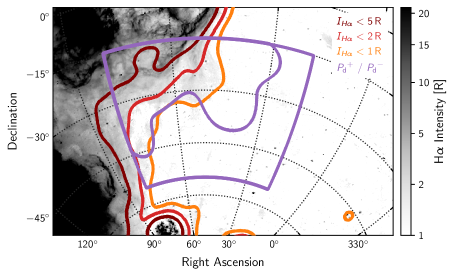
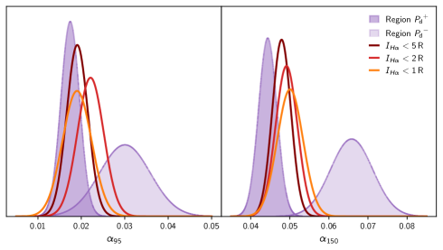
Figure 14: (left) The merged all-sky H$\alpha$ map from Finkbeiner (2003) in units of Rayleighs. The map is smoothed and thresholded at several intensities to create a series of masks (red/orange). The ${P_{\mathrm{d}}}^{+}$ and ${P_{\mathrm{d}}}^{-}$ subregions of the Spider observing region are also overlaid (purple). (right) Plots of $\alpha_{95}$ and $\alpha_{150}$ 1-D likelihoods computed with the XFaster framework for the three Orion-Eridanus Superbubble masks, and compared to the likelihoods for the ${P_{\mathrm{d}}}^{+}$ and ${P_{\mathrm{d}}}^{-}$ regions.

In this Appendix, we assess the impact of the compact structures discussed in Section 3—the Orion-Eridanus Superbubble and the Magellanic Stream—on the detection of spatial variation in the value of $\alpha_{150}$.

Following Soler et al. (2018), we use the full-sky H$\alpha$ map synthesized by Finkbeiner (2003) as a morphological tracer of the Orion-Eridanus Superbubble in the Spider region. In the background map of the left panel of Figure 14, the presence of the Orion-Eridanus Superbubble is evident in the top left corner of our region. To quantify its contribution to the determination of $\alpha_{150}$, we mask the region it occupies with successively more aggressive thresholds. Specifically, for the reasons discussed in Section 3.1, we start by smoothing the Finkbeiner (2003) map with a $5^{\circ}$-FWHM Gaussian. We then build three masks rejecting all pixels in which the H$\alpha$ emission is brighter than 5 R(ayleighs), 2 R, and 1 R, respectively. The threshold-derived borders of these masks, which leave the Spider region with, respectively, 4.39%, 3.81%, and 3.06% of the sky, are shown in the left panel of Figure 14, along with the border of the ${P_{\mathrm{d}}}^{+}$ and ${P_{\mathrm{d}}}^{-}$ subregions ($f_{\mathrm{sky}}\approx 2.4\%$) used in the spatial variation analysis of Section 3. Finally, we compute $\alpha_{95}$ and $\alpha_{150}$ as in Section 3 using the Planck 353 GHz template, but for the full Spider region masked by each of the three H$\alpha$ masks. We chose the Planck 353 GHz template for this analysis because it provides the dominant contribution to the SMICA reconstructed dust map, as shown in Figure 1. Results from these subregions are shown in the right panel of Figure 14.

The value of $\alpha_{95}$ is quite robust to the choice of a Superbubble mask. In fact, the least aggressive mask results in the same value of $\alpha_{95}$ as the most aggressive mask, a value which remains consistent with that determined in the ${P_{\mathrm{d}}}^{+}$ region. Similarly, although the value of $\alpha_{150}$ trends higher as we mask more aggressively—i.e., it trends towards its value in the ${P_{\mathrm{d}}}^{-}$ region—it remains largely consistent with its value in the ${P_{\mathrm{d}}}^{+}$ region, with the ${P_{\mathrm{d}}}^{+}$ and I < 1R results in agreement at $1.4\,\sigma$.

Therefore, the presence of the Orion-Eridanus Superbubble in the Spider region does not appear to drive the detected variation in the value of $\alpha_{150}$.

The Magellanic Stream, which falls mostly outside of the Spider region aside from a few high-velocity clouds (HVCs) along the edge of its bottom right corner, also does not appear to be driving the detected spatial variation in the value of $\alpha_{150}$. Indeed, none of the H$\alpha$ masks shown in Figure 14 exclude the HVCs. Nevertheless, the values of $\alpha_{150}$ derived in the full Spider region after application of any of these masks are consistent with each other, but inconsistent with those found in the ${P_{\mathrm{d}}}^{-}$ region, in which the HVCs also remain. If HVCs were the cause of the detected spatial variation in $\alpha_{150}$, we would expect these four results to be in agreement.

Appendix B Conversion between template $\alpha$ and spectral index $\beta$

Galactic dust emission is modeled as a single MBB with a power-law emissivity,

$$I(\nu)=\tau_{0}\left(\frac{\nu}{\nu_{0}}\right)^{\beta}B(\nu,T),$$ (B1)

where $\tau_{0}$ is the optical depth at the reference frequency $\nu_{0}$. Throughout the text, we use $\beta_{\mathrm{d}}$ and $T_{\mathrm{d}}$ to refer to the spectral index and temperature of the dust component as defined in Equation B1. We calculate an effective observing frequency using the dust SED that takes into account the bandpass of the observing instrument. In general,

$$\bar{\nu}=\frac{\int d\nu\;\nu I(\nu)t(\nu)}{\int d\nu\;I(\nu)t(\nu)},$$ (B2)

where $I(\nu)$ is the SED of the observed source and $t(\nu)$ is the spectral transmission of the detector, properly normalized to its optical efficiency $\epsilon$. This equation is a generalization of Equation 4 of Planck Collaboration et al. (2014). There, they express $I(\nu)$ for a power-law like SED: $I(\nu)\sim\left(\nu/\nu_{0}\right)^{\alpha_{Pl}}$. Note that we identify the spectral index for this simple SED as $\alpha_{Pl}$ to differentiate it from the template coefficients $\alpha_{95}$ and $\alpha_{150}$ used throughout the main text.

Table 2: Effective Planck and Spider band centers in GHz for different input SED models. Band center labels correspond to the CMB and dust models used throughout the main text.

		Planck				Spider
SED Description	Label	100 GHz	143 GHz	217 GHz	353 GHz	95 GHz	150 GHz
Flat $I(\nu)=1$	$\bar{\nu}^{\mathrm{CMB}}$	101.2	142.6	221.4	360.6	94.8	150.8
$\alpha_{Pl}=4$		105.1	148.1	228.8	371.4	96.9	154.0
MBB ($\beta_{\mathrm{d}}=1.53,T_{\mathrm{d}}=19.6\,\mathrm{K}$)	$\bar{\nu}^{\mathrm{d}}$	104.5	147.2	227.3	368.8	96.6	153.5
MBB ($\beta_{\mathrm{d}}=1.59,T_{\mathrm{d}}=22.0\,\mathrm{K}$)		104.5	147.3	227.5	369.1	96.6	153.5

Table 2 lists effective frequency band centers for a variety of SED models. The results presented in Planck Collaboration et al. (2014) assume the $\alpha_{Pl}=4$ SED. However, this assumption holds true only in the Rayleigh-Jeans limit, and only when $\beta\approx 2$. A more accurate effective frequency can be calculated by considering the true dust SED.

CMB maps are typically shown in so-called thermodynamic units ($\mu K_{\mathrm{CMB}}$), which encode the amplitude of fluctuations about the CMB temperature, $T_{\mathrm{CMB}}=2.725$ K. The amplitude of dust emission can be expressed in these units by normalizing the dust emissivity with a first-order Taylor expansion of the CMB blackbody emission about $T=T_{\mathrm{CMB}}$:

$$\Delta T(\bar{\nu}^{\mathrm{d}})=\left(\left.\frac{\partial B}{\partial T}\right|_{T=T_{\mathrm{CMB}}}\right)^{-1}I(\bar{\nu}^{\mathrm{d}})=\frac{(e^{x}-1)^{2}}{x^{2}e^{x}}\frac{1}{2k}\left(\frac{c}{\bar{\nu}^{\mathrm{CMB}}}\right)^{2}I(\bar{\nu}^{\mathrm{d}}).$$ (B3)

Here, for convenience, we have defined $x\equiv h\bar{\nu}^{\mathrm{CMB}}/(kT_{\mathrm{CMB}})$. This equation describes the anisotropy in the mm-map caused by dust emission. It is important to note that the effective frequency used for conversion to thermodynamic units ($\bar{\nu}^{\mathrm{CMB}}$) differs from the effective frequency used for the dust scaling ($\bar{\nu}^{\mathrm{d}}$). The map-domain scaling relationship from a reference frequency $\nu_{0}$ to a lower frequency $\nu$ is then expressed as

$$A\left(\bar{\nu}^{\mathrm{d}},\bar{\nu}_{0}^{\mathrm{d}};\beta_{\mathrm{d}},T_{\mathrm{d}}\right)=\frac{\Delta T(\bar{\nu}^{\mathrm{d}})}{\Delta T(\bar{\nu}_{0}^{\mathrm{d}})}=\frac{(e^{x}-1)^{2}}{x^{2}e^{x}}\frac{x_{0}^{2}e^{x_{0}}}{(e^{x_{0}}-1)^{2}}\left(\frac{\bar{\nu}_{0}^{\mathrm{CMB}}}{\bar{\nu}^{\mathrm{CMB}}}\right)^{2}\left(\frac{\bar{\nu}^{\mathrm{d}}}{\bar{\nu}_{0}^{\mathrm{d}}}\right)^{\beta_{\mathrm{d}}}\frac{B(\bar{\nu}^{\mathrm{d}},T_{\mathrm{d}})}{B(\bar{\nu}_{0}^{\mathrm{d}},T_{\mathrm{d}})}.$$ (B4)

Because we construct dust templates from Planck difference maps, specifically $353-100$ GHz or $217-100$ GHz, there is a minor subtraction of dust at $100$ GHz. Consequently, the scaling of the difference template to a frequency $\nu$ is thus given by

$$\alpha\left(\bar{\nu}^{\mathrm{d}},\bar{\nu}_{0}^{\mathrm{d}};\beta_{\mathrm{d}},T_{\mathrm{d}}\right)=\frac{\Delta T(\bar{\nu}^{\mathrm{d}})}{\Delta T(\bar{\nu}_{0}^{\mathrm{d}})-\Delta T(\bar{\nu}_{100}^{\mathrm{d}})}=\frac{A\left(\bar{\nu}^{\mathrm{d}},\bar{\nu}_{0}^{\mathrm{d}};\beta_{\mathrm{d}},T_{\mathrm{d}}\right)}{1-A\left(\bar{\nu}_{100}^{\mathrm{d}},\bar{\nu}_{0}^{\mathrm{d}};\beta_{\mathrm{d}},T_{\mathrm{d}}\right)},$$ (B5)

where $\bar{\nu}_{100}^{d}=104.5$ GHz according to Table 2. To recover a value of $\beta_{\mathrm{d}}$ given $\alpha$, Equation B5 must be inverted using numerical methods.

Appendix C Comparison to All PySM3 Dust Models

Section 6 and Figure 13 present a comparison between PySM3 dust models and the dust component estimated by SMICA. For simplicity, that comparison used only a representative subset of the available models. The remaining ones are shown in Figure 15.

Due to the fact that both the Spider SMICA results and the PySM3 models incorporate—to varying extents—both the Planck data and noise simulations, the covariance between them is non-trivial. While this makes a quantitative measure of the goodness of fit between the Spider data and the models difficult to assess, we reiterate that the overall amplitude of the Spider SMICA result is driven by the Spider 95 and 150 GHz data, and is therefore largely independent from the amplitude of the models shown. The amplitudes of the d9–d11 family of models are in closest agreement with the SMICA amplitudes at 150 GHz. Most other models predict more power than Spider, except d12, which predicts significantly less.

For convenience, we provide a brief description of the PySM3 dust models shown in Figure 15. For a definitive description we refer the reader to the official documentation.

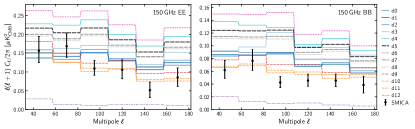
Figure 15: Companion to Figure 13 with the remaining PySM3 dust models. As before, this compares the $EE$ (left) and $BB$ (right) spectra from the PySM3 dust models (colored lines) to SMICA-derived dust bandpowers at 150 GHz (black points) in the Spider region. Models based on the same underlying inputs and class of SED modeling are shown with the same line style. Models drawn with thinner lines are those already shown in Figure 13.

Models d0–d4

This family of models treats thermal dust emission as a single-component modified black body (MBB). Polarized dust templates are based on the Planck 353 GHz channel, and are scaled to other frequencies using an MBB spectral energy distribution (SED). The polarization templates are smoothed with a Gaussian kernel of $2.6^{\circ}$ FWHM, with power at smaller scales added according to the model described in the reference. For the SED, the models use:

d0

A spatially fixed spectral index $\beta_{\mathrm{d}}=1.54$ and a black body temperature, $T_{\mathrm{d}}=20$K.

d1

A spatially varying spectral index and temperature based upon those provided in the Planck Commander maps (Planck Collaboration et al., 2016b), which assume the same spectral index for both intensity and polarization.

d2 (d3)

An emissivity index that varies spatially on degree scales, drawn from a Gaussian with $\beta=1.59\pm 0.2~{}(0.3)$.

d4

The two component (one hot, one cold) dust model of Finkbeiner et al. (1999).

Models d5, d7, d8

Implementations of the model described in Hensley & Draine (2017), using:

d5

The baseline model of that reference.

d7

A model including iron inclusions in the grain composition.

d8

A simplified version of d7 in which the interstellar radiation field strength is uniform.

Model d6

A model that averages over spatially varying dust spectral indices, both unresolved and along the line of sight, using the frequency covariance of Vansyngel et al. (2017) to calculate the frequency dependence.

Models d9–d11

A family of models using a single component MBB with templates based on the Planck GNILC analysis (Planck Collaboration et al., 2020a), using the 353 GHz color correction described in (Planck Collaboration et al., 2020b). The frequency modeling uses:

d9

A fixed spectral index $\beta_{\mathrm{d}}=1.48$ and temperature $T_{\mathrm{d}}=19.6$K.

d10

Additional small scale fluctuations in the template, as well as the dust spectral index and temperature.

d11

Identical to d10, but using a different set of seeds and maximum multipole to generate the small scale features.

Model d12

A three-dimensional model of Galactic dust emission based on Martínez-Solaeche et al. (2018).

References

- Abazajian et al. (2016) Abazajian, K. N., et al. 2016, arXiv:1610.02743
- Adam et al. (2016) Adam, R., Ade, P. A., Aghanim, N., et al. 2016, Astronomy & Astrophysics, 594, A10
- Balkenhol et al. (2023) Balkenhol, L., Dutcher, D., Mancini, A. S., et al. 2023, Physical Review D, 108, 023510
- BICEP2/Keck, Planck Collaborations et al. (2015) BICEP2/Keck, Planck Collaborations, Ade, P. A. R., Aghanim, N., et al. 2015, Phys. Rev. Lett., 114, 101301. https://link.aps.org/doi/10.1103/PhysRevLett.114.101301
- BICEP/Keck Collaboration et al. (2021) BICEP/Keck Collaboration, Ade, P. A. R., Ahmed, Z., et al. 2021, Phys. Rev. Lett., 127, 151301
- BICEP/Keck Collaboration et al. (2023) —. 2023, ApJ, 945, 72
- Brandt et al. (1994) Brandt, W. N., Lawrence, C. R., Readhead, A. C. S., Pakianathan, J. N., & Fiola, T. M. 1994, ApJ, 424, 1
- Caldwell et al. (2017) Caldwell, R. R., Hirata, C., & Kamionkowski, M. 2017, The Astrophysical Journal, 839, 91. https://dx.doi.org/10.3847/1538-4357/aa679c
- Cardoso et al. (2008) Cardoso, J.-F., Le Jeune, M., Delabrouille, J., Betoule, M., & Patanchon, G. 2008, IEEE Journal of Selected Topics in Signal Processing, 2, 735
- Chon et al. (2004) Chon, G., Challinor, A., Prunet, S., Hivon, E., & Szapudi, I. 2004, Monthly Notices of the Royal Astronomical Society, 350, 914
- Clark et al. (2021) Clark, S., Kim, C.-G., Hill, J. C., & Hensley, B. S. 2021, The Astrophysical Journal, 919, 53
- Draine & Fraisse (2009) Draine, B. T., & Fraisse, A. A. 2009, ApJ, 696, 1
- Draine & Li (2007) Draine, B. T., & Li, A. 2007, ApJ, 657, 810
- Dunkley et al. (2009) Dunkley, J., Amblard, A., Baccigalupi, C., et al. 2009, in American Institute of Physics Conference Series, Vol. 1141, CMB Polarization Workshop: Theory and Foregrounds: CMBPol Mission Concept Study, ed. S. Dodelson, D. Baumann, A. Cooray, J. Dunkley, A. Fraisse, M. G. Jackson, A. Kogut, L. Krauss, M. Zaldarriaga, & K. Smith, 222–264
- Finkbeiner (2003) Finkbeiner, D. P. 2003, The Astrophysical Journal Supplement Series, 146, 407. https://doi.org/10.1086%2F374411
- Finkbeiner et al. (1999) Finkbeiner, D. P., Davis, M., & Schlegel, D. J. 1999, The Astrophysical Journal, 524, 867
- Galliano et al. (2018) Galliano, F., Galametz, M., & Jones, A. P. 2018, ARA&A, 56, 673
- Gambrel et al. (2021) Gambrel, A. E., Rahlin, A. S., Song, X., et al. 2021, ApJ, 922, 132
- Gorski et al. (2005) Gorski, K. M., Hivon, E., Banday, A., et al. 2005, The Astrophysical Journal, 622, 759
- Hazumi et al. (2020) Hazumi, M., Ade, P. A., Adler, A., et al. 2020, in Space Telescopes and Instrumentation 2020: Optical, Infrared, and Millimeter Wave, ed. M. Lystrup, N. Batalha, E. C. Tong, N. Siegler, & M. D. Perrin (SPIE). http://dx.doi.org/10.1117/12.2563050
- Hensley & Bull (2018) Hensley, B. S., & Bull, P. 2018, ApJ, 853, 127
- Hensley & Draine (2017) Hensley, B. S., & Draine, B. T. 2017, The Astrophysical Journal, 834, 134. https://dx.doi.org/10.3847/1538-4357/834/2/134
- Hensley & Draine (2022) Hensley, B. S., & Draine, B. T. 2022, arXiv e-prints, arXiv:2208.12365
- Hensley et al. (2022) Hensley, B. S., Clark, S. E., Fanfani, V., et al. 2022, The Astrophysical Journal, 929, 166. http://dx.doi.org/10.3847/1538-4357/ac5e36
- HI4PI Collaboration et al. (2016) HI4PI Collaboration, Ben Bekhti, N., Flöer, L., et al. 2016, A&A, 594, A116
- Hogg et al. (2010) Hogg, D. W., Bovy, J., & Lang, D. 2010, arXiv e-prints, arXiv:1008.4686
- Huffenberger et al. (2020) Huffenberger, K. M., Rotti, A., & Collins, D. C. 2020, The Astrophysical Journal, 899, 31. https://dx.doi.org/10.3847/1538-4357/ab9df9
- Hurier et al. (2013) Hurier, G., Macías-Pérez, J. F., & Hildebrandt, S. 2013, A&A, 558, A118
- Kamionkowski & Kovetz (2016) Kamionkowski, M., & Kovetz, E. D. 2016, Annual Review of Astronomy and Astrophysics, 54, 227. https://doi.org/10.1146/annurev-astro-081915-023433
- Kandel et al. (2017) Kandel, D., Lazarian, A., & Pogosyan, D. 2017, Monthly Notices of the Royal Astronomical Society: Letters, 472, L10. https://doi.org/10.1093/mnrasl/slx128
- Leung et al. (2022) Leung, J. S.-Y., Hartley, J., Nagy, J. M., et al. 2022, The Astrophysical Journal, 928, 109. http://dx.doi.org/10.3847/1538-4357/ac562f
- Li & Draine (2001) Li, A., & Draine, B. T. 2001, ApJ, 554, 778
- Loken et al. (2010) Loken, C., Gruner, D., Groer, L., et al. 2010, in Journal of Physics: Conference Series, Vol. 256, IOP Publishing, 012026
- Martínez-Solaeche et al. (2018) Martínez-Solaeche, G., Karakci, A., & Delabrouille, J. 2018, Monthly Notices of the Royal Astronomical Society, 476, 1310
- Mathewson et al. (1974) Mathewson, D. S., Cleary, M. N., & Murray, J. D. 1974, ApJ, 190, 291
- Page et al. (2007) Page, L., Hinshaw, G., Komatsu, E., et al. 2007, ApJS, 170, 335
- Pelgrims et al. (2021) Pelgrims, V., Clark, S. E., Hensley, B. S., et al. 2021, A&A, 647, A16
- Planck Collaboration (2016) Planck Collaboration. 2016, Astronomy & Astrophysics, 594, A10
- Planck Collaboration et al. (2014) Planck Collaboration, Ade, P. A. R., Aghanim, N., et al. 2014, A&A, 571, A9
- Planck Collaboration et al. (2016a) Planck Collaboration, Adam, R., Ade, P. A. R., et al. 2016a, A&A, 586, A133
- Planck Collaboration et al. (2016b) —. 2016b, Astronomy & Astrophysics, 594, A10
- Planck Collaboration et al. (2020a) Planck Collaboration, Akrami, Y., Ashdown, M., et al. 2020a, A&A, 641, A4
- Planck Collaboration et al. (2020b) —. 2020b, A&A, 641, A11
- Planck Collaboration et al. (2020c) Planck Collaboration, Aghanim, N., Akrami, Y., et al. 2020c, A&A, 641, A3
- Planck Collaboration et al. (2020d) Planck Collaboration, Aghanim, N., Akrami, Y., et al. 2020d, Astronomy & Astrophysics, 641, A12. https://doi.org/10.1051/0004-6361/201833885
- Plaszczynski et al. (2014) Plaszczynski, S., Montier, L., Levrier, F., & Tristram, M. 2014, MNRAS, 439, 4048
- Poh & Dodelson (2017) Poh, J., & Dodelson, S. 2017, Phys. Rev. D, 95, 103511. https://link.aps.org/doi/10.1103/PhysRevD.95.103511
- Purcell (1975) Purcell, E. M. 1975, in The Dusty Universe, ed. G. B. Field & A. G. W. Cameron, 155–167
- Remazeilles et al. (2016) Remazeilles, M., Dickinson, C., Eriksen, H. K. K., & Wehus, I. K. 2016, Monthly Notices of the Royal Astronomical Society, 458, 2032. https://doi.org/10.1093/mnras/stw441
- Ritacco et al. (2023) Ritacco, A., Boulanger, F., Guillet, V., et al. 2023, A&A, 670, A163. https://doi.org/10.1051/0004-6361/202244269
- Seljak & Zaldarriaga (1997) Seljak, U., & Zaldarriaga, M. 1997, Phys. Rev. Lett., 78, 2054
- Soler et al. (2018) Soler, J. D., Bracco, A., & Pon, A. 2018, Astronomy & Astrophysics, 609, L3. https://doi.org/10.1051%2F0004-6361%2F201732203
- SPIDER Collaboration et al. (2022) SPIDER Collaboration, Ade, A. R., Amiri, M., et al. 2022, The Astrophysical Journal, 927, 174. https://dx.doi.org/10.3847/1538-4357/ac20df
- Tassis & Pavlidou (2015) Tassis, K., & Pavlidou, V. 2015, MNRAS, 451, L90
- The Simons Observatory Collaboration et al. (2019) The Simons Observatory Collaboration, Ade, P., Aguirre, J., et al. 2019, Journal of Cosmology and Astroparticle Physics, 2019, 056
- Thorne et al. (2017) Thorne, B., Dunkley, J., Alonso, D., & Næss, S. 2017, Monthly Notices of the Royal Astronomical Society, 469, 2821. http://dx.doi.org/10.1093/mnras/stx949
- Vansyngel et al. (2017) Vansyngel, F., Boulanger, F., Ghosh, T., et al. 2017, A&A, 603, A62
- Wright et al. (1991) Wright, E. L., Mather, J. C., Bennett, C. L., et al. 1991, ApJ, 381, 200