2D Skyrmion topological charge of spin textures with arbitrary boundary conditions: a two-component spinorial BEC as a case study
Abstract
We derive the most general expression for the Skyrmion topological charge for a two-dimensional spin texture, valid for any type of boundary conditions or for any arbitrary spatial region within the texture. It reduces to the usual one for the appropriate boundary conditions, with the spin texture. The general expression resembles the Gauss-Bonet theorem for the Euler-Poincaré characteristic of a 2D surface, but it has definite differences, responsible for the assignment of the proper signs of the Skyrmion charges. Additionally, we show that the charge of a single Skyrmion is the product of the value of the normal component of the spin texture at the singularity times the Index or winding number of the transverse texture, a generalization of a Poincaré theorem. We illustrate our general results analyzing in detail a two-component spinor Bose-Einstein condensate in 2D in the presence of an external magnetic field, via the Gross-Pitaevskii equation. The condensate spin textures present Skyrmions singularities at the spatial locations where the transverse magnetic field vanishes. We show that the ensuing superfluid vortices and Skyrmions have the same value for their corresponding topological charges, in turn due to the structure of the magnetic field.
Keywords: Skyrmion charge, Vortices, BEC, Ultracold Quantum Matter
I Introduction
Skyrmions are topological defects or excitations that emerge in continuous fields and spin textures due to intrinsic chiral interactions or to the presence of external inhomogeneous magnetic or gauge fields. These excitations arise in diverse materials or fields as in nuclear physics Skyrme (1961); Adkins et al. (1983); Meissner and Zahed (1986), particle physics Holzwarth and Schwesinger (1986); Schwesinger et al. (1989), notably in magnetic systems in condensed matter, such as in 2D electron gas Brey et al. (1995), magnetic metals Rößler
et al. (2006); Hoffmann et al. (2017); Romming et al. (2013), transition metal films Dupé et al. (2014), frustrated magnets Leonov and Mostovoy (2015) and in a host of other magnetic situations Nagaosa and Tokura (2013); Jalil and Tan (2014), liquid crystals Wright and Mermin (1989); Leonov et al. (2014) and, the context of the present paper, in Bose-Einstein condensates, both 2D Al Khawaja and Stoof (2001); Kasamatsu et al. (2005); Leanhardt et al. (2003); Pietilä and Möttönen (2009); Leslie et al. (2009); Choi et al. (2012a); Su et al. (2012); Xu and Han (2012); LIU et al. (2013); Huang and Yip (2013); Choi et al. (2012b); Hu et al. (2015); Lovegrove et al. (2016); Borgh et al. (2016); Dong et al. (2017); Zamora-Zamora and Romero-Rochín (2018); Liu et al. (2024) and 3D Marzlin et al. (2000); Ruostekoski and Anglin (2001); Battye et al. (2002); Mizushima et al. (2002); Pietilä et al. (2007); Kawakami et al. (2012); Liu et al. (2013); Luo et al. (2019); Chen et al. (2022); Tiurev et al. (2018). Ever since Skyrme seminal work Skyrme (1961), its analysis has been pursued in field theoretical models such as the non-linear -model in high energy physics Adkins et al. (1983); Meissner and Zahed (1986); Wilczek and Zee (1983), or in terms of the Dzyaloshinskii-Moriya theory in magnetic systems Dzyaloshinsky (1958); Moriya (1960), or within the Gross-Pitaevskii (GP) equation in Bose-Einstein condensates, as in essentially all of the theoretical works already referenced. In this paper we deal with Skyrmions generated by an external gauge field in a two-component spinorial Bose-Einstein condensate in two spatial dimensions, described by two coupled GP equations. This stylized model allows for a simple and clear description of spin textures that can show a rich variety of Skyrmions, with the allowance for the determination of all its inherent and topological properties. In most of the experimental Skyrmion realizations, BEC studies have been performed in real alkaline weakly interacting Bose clouds with spin Leanhardt et al. (2003); Choi et al. (2012b, a); Su et al. (2012) and Leslie et al. (2009), however, the topological properties of a given spin structure should be independent of their physical origin.
An outstanding feature of Skyrmions is their topological character ingrained and described by its topological charge. In most of the studies on 2D Skyrmions the topological charge has been considered to be given by the expression Wilczek and Zee (1983); Kasamatsu et al. (2005); Heinze et al. (2011); Romming et al. (2013); Choi et al. (2012b); Hu et al. (2015); Lovegrove et al. (2016); Dong et al. (2017); Choi et al. (2012a); Pietilä and Möttönen (2009); Dupé et al. (2014); Shnir (2018)
| (1) |
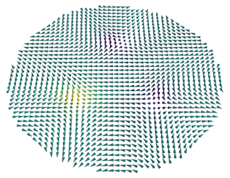
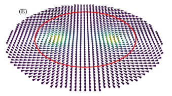
where is the 3D vector spin texture or continuous field of the problem at hand, obeying everywhere in the -plane. It is expected that the charge is an integer. This expression, however, requires particular boundary conditions. Skyrme Skyrme (1961) and others afterwards Wilczek and Zee (1983); Kasamatsu et al. (2005); Shnir (2018) considered that constant as and, in such a case, is a positive or negative multiple integer, with the interpretation that is the number of times the mapping of covers the unit sphere. Additionally, if the spin texture lies on the plane at the boundary, then , a defect called a half Skyrmion Su et al. (2012); Leslie et al. (2009); Choi et al. (2012a); LIU et al. (2013); Zamora-Zamora and Romero-Rochín (2018). These boundary conditions, however, need not appear or exist in a given physical problem Zamora-Zamora and Romero-Rochín (2018) or in a multiple Skyrmion configuration, where one may need to evaluate the local charge of the Skyrmions present. In these cases expression (1) cannot account for the calculation of the whole charge that, from topological consideration, must be an integer. As an example, in figure 1 we present a spin texture arising in the 2D spin 1/2 spinor Bose-Einstein condensate (BEC) here studied, the details of such a solution given further below. We observe a configuration of three Skyrmions, one pointing on the positive -direction and the other two in the negative one. Each defect should have its own topological charge, properly defined, and the total one of the full configuration should be the sum of the individual ones. The main purpose of this article is to show that a topological charge of the whole or part of the spin texture configuration can be defined within an arbitrary closed curve, which may or may not be the true boundary of the spin texture. Parametrizing the curve by , with and , we will find that such a topological charge is given by
| (2) | |||||
with , a positive or negative integer. The first term is the usual one, except for a factor of 2, with the area enclosed by the curve . The second is a boundary term with the integral along the curve , and the third one takes into account the possible fact that the vector , tangent to the parametric 3D curve ,
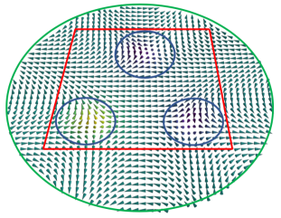
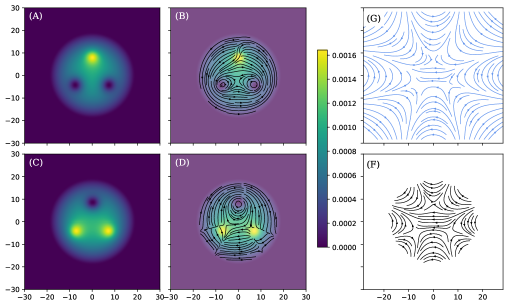
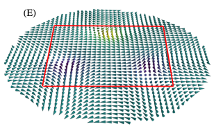
may be discontinuous at a finite number of points along the curve. All these aspects should become clearer in the derivation given below. The above expression indeed reduces to the usual one for the boundary conditions described in the previous paragraph. Figure 2 shows the same spin texture as in figure 1 but with several boundary curves . The small circular ones each enclose the local Skyrmion singularities, yielding for the two of them pointing down and for the one pointing up, using (2). The large circle and the square curve enclose the three Skyrmions and yield , which is the sum of the local ones. We remark that, for the square curve, the last term of (2) must be taken into account since it gives rise to discontinuities on the tangent vector mentioned above.
While we claim that the above expression is a general one for any spin texture, since the derivation that we provide makes no reference to the physical origin of the spin texture, for purposes of illustrations and for a better understanding of the Skyrmion charge, we will use the spin textures arising from a spinorial BEC in the presence of an external magnetic field, as a case study. In addition, an important and interesting point, is that such a system shows another well known type of topological defects, namely, quantum vortices Kasamatsu et al. (2005); Lin et al. (2009a); Kawaguchi and Ueda (2012); Zamora-Zamora et al. (2012); Stamper-Kurn and Ueda (2013); Ueda (2014). We will explicitly show the profound relationship between the quantum vortices and the Skyrmions, namely, that their corresponding local charges have exactly the same values. The present stylized model allows for finding that, for the present problem, the external magnetic or gauge field ultimately defines the topological structure of the vortices and the Skyrmions.
The article is organized as follows. In Sections II and III we present a detailed analysis, both in a simplified analytic and in a full numerical fashion, of stationary solutions to the Gross-Pitaevskii equations of a 2D 1/2 spinorial Bose gas in the presence of an external inhomogeneous magnetic field. We show how the quantum vortices and Skyrmions can be predicted from the knowledge of the magnetic field. In Section IV, the main contribution of this article, we provide a general derivation of the topological charge of Skyrmions present in any given spin texture, for arbitrary boundary curves. Section V is devoted to a discussion between the similarities and discrepancies between the Skyrmions topological charge and the Euler-Poincaré characteristic of a surface in terms of the Gauss-Bonet theorem Weatherburn (1930); Kreyszig (1991); McCleary (1997); do Carmo (2016). In an Appendix we illustrate our main result with a variety of numerical solutions of different spin textures generated by different magnetic fields, and for different types of arbitrary boundary curves. Final remarks are given in Section VI.
II 1/2 Spinor BEC in the presence of an external magnetic field
We consider stationary states of a two-component spinorial BEC in 2D, with a Zeeman coupling to an external magnetic field, as described by the coupled Gross-Pitaevskii (GP) equations
| (3) |
where and denotes the two components of the spinor. Summing over repeated indices is assumed. is the chemical potential and the magnetic dipole operator is given by
| (4) |
where are Pauli matrices and the magnitude of the magnetic dipole moment. The magnetic field is
| (5) |
We denote as the transverse magnetic field and, for simplicity, we will consider constant . We choose such that it vanishes at certain points . We shall see that at those points there appear quantum vortices and the origins of Skyrmions Zamora-Zamora et al. (2012). The normalization condition is
| (6) |
Writing the solution as , the superfluid density and the superfluid velocity , in each component, are given by
| (7) | |||||
| (8) |
The circulation of the velocity field in an arbitrary closed circuit is defined by
| (9) |
As we will explicitly calculate, if the circuit does not enclose a quantum vortex the circulation vanishes, but when a vortex or vortices are enclosed, the circulation yields the vortex topological charge within the circuit Ueda (2014); Zamora-Zamora et al. (2012)
| (10) |
with , a positive or negative integer.
The condensate spin texture is an observable, independent of the spin basis, and defined at any spatial point within the condensate,
| (11) |
It can be verified that the spin texture has magnitude one everywhere.
Writing , the components explicitly are
| (12) |
III Vortices and Skyrmions in the vicinity of points of vanishing transverse magnetic field
While we will consider a variety of magnetic fields, all have in common that they have spatial points where the transverse magnetic field vanishes, . This property imprints both the appearance of vortices and of Skyrmions at those points. To understand how this occurs, with no loss of generality, we consider a transverse magnetic field that vanishes at the origin and analyze the behavior of the spinor wavefunctions in its vicinity. For this we explicitly write both GP equations for the two spinor components, assuming that ,
| (13) |
where and . In the vicinity of the origin the magnetic field generically vanishes as Zamora-Zamora et al. (2012)
| (14) |
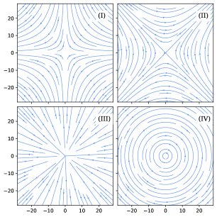
where is the field strength, not necessarily real, and a positive integer. We note that if is real, the resulting field obeys and , namely, it would be a true magnetic field. However, one can consider arbitrary “artificial” gauge fields Lin et al. (2009b); Dalibard et al. (2011) that do not necessarily satisfy Maxwell equations but that allow for different sorts of fields and which in turn give rise to different spin textures, as we show in the rest of the paper. In this way, generically, there are four different types of fields in the vicinity of a vanishing location, with real, positive or negative,
| (15) |
The first two obey Maxwell equations, the last two do not; as a matter of fact, case (I) with is commonly produced in a Ioffe-Pritchard trap, and is a quadrupole trap Leanhardt et al. (2003). Figure (3) shows the structure of the magnetic fields for the case . Case (III) is the hedgehog configuration usually considered in Skyrmion discussions Wilczek and Zee (1983); Shnir (2018).
As we will see, the local structure of the transverse magnetic field at its vanishing points plays a fundamental role in the final signs of the topological charges of the vortices and Skyrmions. As discussed in Section V below, such a structure can be associated to a topological quantity, namely, the Index of the field at the vanishing point. do Carmo (2016)
Let us consider case (I) for the moment. We will summarize all cases below. For this case there are two possible solutions,
| (16) |
Substitution of these solution into GP equations (13) shows that, very near , one obtains
| (17) |
where is a positive constant that can be numerically determined. The important features are that vanishes as while yields a constant as . Therefore, case (i) in (18) is a vortex in the component and a density “spike” in the one (see below), and the opposite in (ii), namely a spike in and a vortex in . As we see now, in the former case the vortex charge is , while in the latter . This can be concluded right away from the velocity fields,
| (18) |
where . Indeed, the velocity fields circulate in the clockwise (negative) direction in the component for case (i), and in the anticlockwise (positive) direction for the one, in case (ii). The circulations are, using a circular contour of radius and ,
| (19) | |||||
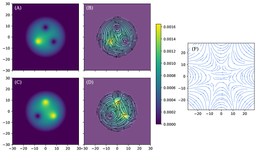
finding the values of the topological charges already quoted. Clearly, if the vortex is not enclosed by the contour, the circulation vanishes, . Figure 4 shows the solution to the GP equations (13), as well as the velocity fields, corresponding to figures (1) and (2), including the magnetic field that generates such a configuration; see the Appendix for details of the calculation. One can observe that, in the vicinity of the vortices, the top one is of type (II) while the lower ones are of type (I) in (15). In panels (A) and (C) of 4 we can also see what we mean by a “density spike”: while the vortex in one component occurs, accompanied by a density depletion, in the other component there is a rapid increase of the density at the same spatial location, namely a spike, identified in the figure by a bright spot in the density profile. This increment of the density in one spinor component almost cancels the depletion at the vortex in the other component Zamora-Zamora et al. (2012).
From expressions (15) of the fields, the vortex structure of case (II) is the same as case (I) just discussed, however in cases (III) and (IV) the solution is as in (I) given by (18), but with the velocity circulation reversed and, therefore, the charges are now for solution (i) and for (ii). As we will see below, the Skyrmion charges will have exactly the same values as , with their own spin texture structure.
We now turn our attention to the spin texture and, for the sake of argument, we also study case (I). Again, in the vicinity of zero field, one finds the spin texture from (12), for both solutions (i) and (ii) in (18)
| (20) |
where the signs in front of refer to solutions (i) and (ii), respectively, see (18). First, we note that the transverse spin texture is parallel and in the same direction to the transverse magnetic field , as physically expected, see (I) in (15), thus showing that both have the same spatial pattern. This is true in general and it is exemplified in the gallery of figures in the Appendix.
Evidently, as , the components and vanish since either or vanish as well, and the spin texture becomes parallel to the vector, pointing upwards or downwards, . This latter direction is determined by whether the solution is (i) or (ii) as above in (18): for solution (i) , and, therefore, the spin texture points downwards, ; for solution (ii) , and the spin texture now points upwards, . For the other fields (II), (III) and (IV) the same rule applies for the peaks: if the vortex appears in the component, the texture points downwards, but if the vortex is in then it points upwards. The ensuing structure of the spin texture is what we call the Skyrmion and, for the sake of describing it, we shall call the location where , as the origin of the Skyrmion.
IV The topological charge of the Skyrmions
As mentioned in the Introduction, the topological charge of the Skyrmions is usually given by (1) but, as also argued, such an expression requires particular boundary conditions on the spin texture . As also already mentioned, in general those boundary conditions need not occur, or a spin texture can have a multiplicity of coexisting local Skyrmions, whose boundaries among them can also be quite arbitrary. Moreover, in all cases one should be able to asses the individual charges of the local Skyrmions in order to validate that the charges add as any topological index. The spin textures here presented are clear examples of the just two described situations. There is another fundamental aspect to be considered as well. In descriptions of common spin textures and their charge given by (1), it is affirmed that the topological charge is the number of times that the unit sphere is covered by the spin texture. This follows, on the one hand, by assuming that , being a unit vector, is by itself a parametrization or mapping of the unit sphere and, on the other, again, by the mentioned usual boundary conditions. While such a parametrization can indeed be assumed, there is subtle aspect that we believe has not been addressed before, namely, that different spin textures give rise to mappings to the unit sphere but with different orientations. That is, the normal vector to the sphere, generated by the parametrization , can point outwards or inwards to the sphere, depending on the given spin texture. And, for configurations with several Skyrmions, this can occur within the same spin texture. This is a very interesting and important point to consider in the elucidation of a general expression for the identification of the Skyrmion topological charge. In this section we present a derivation of the Skyrmion topological charge, in an as possible straightforward fashion, by a procedure similar to the derivation of the Gauss-Bonet (GB) theorem Weatherburn (1930); do Carmo (2016); Kreyszig (1991). We will leave the discussion of the mentioned delicate issues to the following section, where we also argue about the similarities or, rather, dissimilarities of the Skyrmion charge with the Euler-Poincaré characteristic , arising from the GB theorem.
Let us assume that a spin texture is given in all or part of the -plane, such that it has a single location where either or . We call this point the origin of the Skyrmion. Consider now an area that encloses this point. The area has a boundary described by a parametrized closed curve
| (21) |
Notice that although the curve is continuous, its tangent may be discontinuous at a finite number of points . Further, and very important, the curve is assumed, one, to run or be oriented in the positive counterclockwise direction and, two, the curve does not cross itself, say the red curve in figure (5).
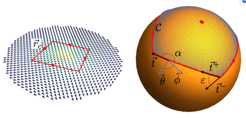
Evidently, since the texture is a unit vector, it can be considered to be the outward normal vector to the unit sphere , with the usual azimuthal and polar sphere angles, (please note that we use for the polar angle in 3D and in 2D)
| (22) |
At the same time one could assume that is by itself a parametrization of the unit sphere. As discussed in detail below why, we will not consider this point of view. As we show below, perhaps surprisingly at first sight, the two mentioned assumptions are not necessarily consistent with each other. Nevertheless, any value of the spin texture can be identified with a single point on the sphere, although the opposite is not true in general. That is, depending on the order of the Skyrmion, parts of the sphere can be covered more than once. Figure (5) shows a simple example of these observations, where we can see how the spin texture within and on the square are mapped to unique points on the sphere. And, with the identification of the unit normal and the spherical angles, the usual orthogonal sphere unit vectors along the directions , can also be expressed in terms of the spin texture,
| (23) |
In an analogous way, we can observe that the curve on the plane gets mapped to a 3D curve , denoted as , that lies on the surface of the unit sphere. The arclength of such a curve can be found from
| (24) |
and the tangent to the curve is given by, see again figure (5) as an example,
| (25) |
This is a unit vector, . Since it is also tangent to the sphere, then and, therefore, lies on the - plane. We define as the positive angle that makes with and, thus, we can write
| (26) |
can take any positive value, see figure 5. Note again that for every texture vector on the curve there is an angle , but the inverse is not necessarily true.
With the above preliminaries we can now start the derivation of the expression for the topological charge of a single Skyrmion. Consider the following integral along the curve ,
| (27) |
Before we proceed with the evaluation of the integral, we note two points. First, while the integrand may seem to be the geodesic curvature of on the sphere, we will see that it is not in general, differing by a minus sign when it is not. And second, although the curve on the plane has been considered to run in the positive counterclockwise direction in the -plane, the curve on the sphere, in general, is not necessarily oriented in the same direction. These apparent discrepancies, to be discussed in the Section V, have their origin in the previous observation that is not being formally considered to be a parametrization of the sphere.
Substituting the tangent vector (26) into the integral (27) yields,
| (28) |
Let us analyze the first integral over the angle. Here it is important to notice that, because of the assumptions on the boundary curve , the tangent to the curve is also discontinuous at the points . This, in turn, implies that the angle is discontinuous at those points: Let be the incoming tangent of the curve at the point and the outgoing one. We call the corresponding angles and . Hence,
| (29) | |||||
where and with . We have assumed that such a point is not on any discontinuity. is the angle between the tangents and at the discontinuity, given by
| (30) |
see figure 5.
Below we return to the analysis of the values of .
The second integral in (28), over the angle , can be rewritten in a way that allows for the determination of another contribution of the Skyrmion charge, using Green theorem. For this, we first recall that the origin of the Skyrmion occurs where the spin texture becomes , that is, where the azimuthal angle equals or , respectively. Since the contour encloses either of those points, the integrand of the second integral in (28) is not analytic at or at , preventing the direct use of Green theorem. However, adding and subtracting an appropriate quantity one obtains
| (31) |
where the sign is used when the singularity is at , namely , and the sign when or . In this way, the integrand of the first integral on the right side of (31) is analytic at the respective points and the integral can be performed using Green Theorem. This yields, up to a sign, the solid angle subtended by the contour around the North or the South Pole,
| (32) |
The sign on the right side depends on the positive or negative orientation of the contour , which in turn depends on the structure of the Skyrmion in the vicinity of the singularity. The above term can also be seen as a Berry phase type contribution Berry (1984). However, the previous integral can be written in a manner that is more appropriate for our purposes, namely, by rewriting it in terms of the spin texture itself:
| (33) | |||||
The first equality follows by writing the angles and in terms of the components, see (22), hence allowing for expressing the line integral along the original contour . The second equality is obtained by means of Green Theorem, the surface integral being performed over the whole area enclosed by the curve . The derivation of the last equality is a laborious exercise that requires the use of . Note that in the expression of the last line one does not need to worry about the sign of the integral, as this will emerge naturally from the current spin texture. The important issue of these signs will be further addressed below.
Collecting the previous results (29), (31) and (33) into (28), we partially obtain
| (34) | |||||
First of all, it is simple to conclude that the left-hand-side of this expression must be
| (35) |
with . This integer will be carefully identified below as the topological charge of the Skyrmion enclosed by the curve . Quite generally, it must be an integer since, first, , then and, hence, with an integer. Similarly, since
| (36) | |||||
with a positive or negative integer, since the contour encloses either the North or the South Pole of the unit sphere. Therefore, is an integer. However, it remains to understand how this integer number relates to the given spin texture and to its behavior in the neighborhood of the singularity .
Let us address the role of the angles and in the determination of the integer value of the Skyrmion charge in (35). First, one can conclude that , namely . This follows from expression (26) for and from the geometrical facts, one, that always points in the direction of increasing , two, that the tangent vector has a definite orientation, counter or clockwise for any given curve and, three, that either the North or South Pole are enclosed by . These three facts imply that the angle retraces itself around without completing a single turn. Thus, this leaves the value of to depend solely on the integral of in (35) and (36). This has an intrinsic topological solution. For this, we write the integral over in terms of an integral of the spin texture over the original contour ,
| (37) |
The interesting and relevant observation if that the integral on the right-hand-side is precisely the Index of the transverse spin texture field , times , around do Carmo (2016). Such an Index is with a positive integer that counts the number of turns the angle does around the corresponding Pole. Based on our findings that the transverse spin texture follows the transverse magnetic field , we can extrapolate and assert that any spin texture, in the vicinity of the singularities = 0, behaves just as the magnetic field given in (15). Hence, for cases (I) and (II) the index is while for (III) and (IV) one obtains . Therefore, in a very general way, the topological charge of a single Skyrmion can be expressed as,
| (38) |
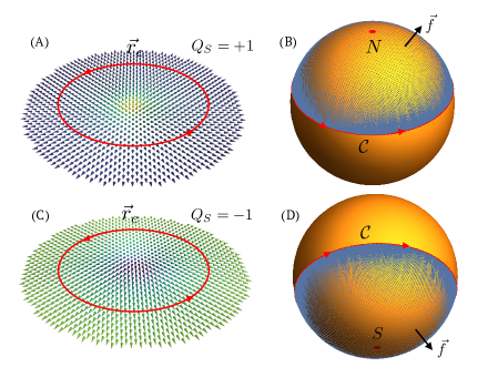
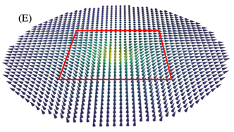
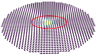
demonstrating that the topological charge is a positive or a negative integer, its sign being determined by both, the value of and the Index of , at the singularity. We believe that this last identification of the Skyrmion charge has not been pointed out before. Figure 6 shows two cases of Skyrmions with singularities at and , produced by the same transverse magnetic field but with opposite component; all the thermodynamic properties are the same, except that the Skymion charges have opposite values.
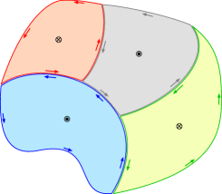
Returning to the identification of in (34), and rewriting the integrals in terms of the spin texture and the original boundary curve , one arrives at the sought for expression for the topological Skyrmion charge given in (2) in the Introduction, but for a single Skyrmion. The extension to the total topological charge of a spin texture that holds an arbitrary number of Skyrmions, whose origins are at , is straightforward. This is achieved with the reasonable assumption that, while in the vicinity of the origins the spin texture behaves as in the case of a single Skyrmion, the “local” textures can be joined smoothly in a continuous and differentiable fashion. This assumption is verified by the numerical examples shown in the Appendix. Very importantly, the boundaries between those local cases can be quite arbitrary and complicated, such as the boundary of our example of the three Skyrmions in figure (1). This corroborates the importance of having obtained the local charge of a Skyrmion for an arbitrary boundary curve . Figure 7 shows a sketch of the union of local boundary curves of several Skyrmions that yields a total curve , inside of which all Skyrmions are enclosed. Writing the different contributions of a local Skyrmion charge as , where
| (39) |
it is evident, since all boundary curves run with same positive orientation, that
| (40) |
with an analogous expression for all contributions , and . The obtained expression for the total Skyrmion charge is given by (2) of the Introduction, with the external boundary curve, , the total area, and the sum over the angles is only on those on the external boundary since all the internal angles cancel out, see figure 7. It is also of interest to conclude that the total Skyrmion charge can be written as,
| (41) |
As we will argue in the following section, this last expression appears as a generalization of Poincaré theorem do Carmo (2016).
In the Appendix we illustrate the results of this section with explicit numerical calculations of several spin textures obtained by solving GP equations (13) for our case study of a spinor BEC in the presence of an external field.
V Dissimilarities between the Skyrmion charge and the Euler-Poincaré characteristic
The expression (2) for the Skyrmion topological charge has a deceivingly similar appearance to the Euler-Poincaré characteristic of the Gauss-Bonet theorem of a given 2D surface embedded in 3D Weatherburn (1930); Kreyszig (1991); McCleary (1997); do Carmo (2016). As a matter of fact, the derivation here presented for is similar, but not equal, to the derivation of the Gauss-Bonet theorem presented by do Carmo do Carmo (2016). However, as we have been alluding to in the text, there are notable differences between them: A technical difference being that the spin texture vector cannot always be both the normal vector and the parametrization to the sphere at the same time. A fundamental difference being that in the Gauss-Bonet theorem the main role is played by the surface itself, while in the Skyrmion case the protagonist is the spin texture .
To be precise, given an orientable surface , the GB theorem states that the Euler-Poincaré characteristic of a region of the surface , with a given closed boundary and with possible exterior angles is, do Carmo (2016)
| (42) |
where is the gaussian curvature at a point on the surface, the geodesic curvature at a point of the curve , the boundary of . The curve must be oriented in the positive direction. These are intrinsic properties of the surface and of curves drawn on it. If the region is a simple region of the surface , then always. If the surface is compact with no boundaries, then where is the genus or number of handles of the surface. And there are surfaces with such as the pseudo sphere and the so-called pair of pants. The above expression for is written in an invariant form, independent of any parametrization of the surface. For sure, one can write it in terms of a parametrization, but this one must be consistent with an assumed orientation of the surface and with the positive orientation of the curve . To see this, let be such a parametrization, then, the normal to the surface is
| (43) |
where is the derivative with respect to . This normal must have the same orientation on the whole surface. For instance, if the surface is a sphere, then must point outwards or inwards over the whole sphere. The gaussian curvature can be expressed as,
| (44) |
Along the same lines, the tangent to the curve is
| (45) |
and, hence, the geodesic curvature of is
| (46) |
The exterior angles are, in an obvious notation,
| (47) |
Therefore, if we compare , from (42)-(47), with from (2), they look quite similar if we identify the parametrization with , the surface thus being a sphere, and the normal with . However, these two identifications are incompatible in general. This can be readily seen if we calculate the normal to the sphere from the parametrization ,
| (48) |
One finds that, depending on the spin texture, or . And this can occur within the same spin texture, such as in the example of figure (1). Therefore, if is a parametrization, then cannot be the normal always, and viceversa. This would result in severe problems since the normal would discontinuously change on the sphere. Hence, we have opted to consider
that is the outward normal to the sphere, at the expense of abandoning as a parametrization. It is then not a surprise that we do not obtain GB theorem and, therefore, is not , since the sign of the former depends on the spin texture and the latter is a topological intrinsic property of the given surface. Indeed, the fact that we can find positive or negative Skyrmion charges, simply by inverting the value of the origin of the Skyrmion is a consequence of not having considered as a parametrization of the sphere. In this way, the integrands of and are not necessarily the gaussian or the geodesic curvatures of the sphere or of the curves drawn on it.
It is also of interest to point out that there is a theorem, due to Poincaré do Carmo (2016), that states that with the Indices of a differentiable vector field on a compact surface with isolated singular points. That is, given the surface, the singularities must exist and their Indices add to . In the present case, see (38), the singularities can be quite arbitrarily given by the the spin texture and, as a consequence, their topological charges depend on an additional sign given by at the singularity.
The previous observations are not definite, however, as we are aware that topology can yield results that may be difficult to visualize geometrically. That is, although we have pointed out evident differences between the Skyrmion topological charge and the Euler-Poincaré characteristic, we also concede that their respective expressions appear strikingly similar. Hence, we leave open the question of whether they may truly be the same topological object or not, perhaps for not so obvious or evident surfaces such as the unit sphere. This should be the subject of further scrutiny. Along the same lines, an approach in terms of homotopy theory Ueda (2014); Schwarz (1994); Mermin (1979) should complement our approach, basically rooted in differential geometry.
VI Final Remarks
In this article we have provided a derivation of the Skyrmion topological charge of an arbitrary spatial region of a spin texture , given by (2). If the spin texture is continuous and differentiable everywhere, except perhaps at the origins of the Skyrmions, where , one can find the local topological charges of the present Skyrmions and, simply by joining the local regions, one can calculate the topological charge of several Skyrmion regions and, eventually, of the whole area where the spin texture is defined. While we can calculate the topological charge as the sum of the three main contributions , one can also demonstrate that the local Skyrmion charge is the product , with the Index of the transverse spin texture at the singularity . The total Skyrmion charge of a region, or of the whole spin texture, is the addition of the local Skyrmion charges. It may be of formal interest to highlight that the 2D contribution , the 1D and the 0D are all expressed in terms of a triple scalar product involving the spin texture times the relevant cross product of the contribution at hand. We also find that, depending on the value of the spin texture at the boundary curve or curves, one recovers the usual expression for the Skyrmion charge, given solely in terms of the contribution . For instance, if the texture completely covers the sphere, , or at the boundary, the last two terms in (2) or (34) vanish. Notice also that we have defined the Skyrmion charge with a factor in (2), instead of as in (1), because of the similarities with the Gauss-Bonet representation of the Euler-Poincare characteristic. Thus, while usually the Skyrmion charge for a closed sphere is , here it is , and as the charge of a half Skyrmion is considered , here it is a . As we indicated in the Introduction, the derived expression is quite general and independent of the origin of the spin texture.
In order to produce spin texture within a physically sensible system, we have studied a 1/2 spinor BE condensate in the presence of an external magnetic field. This system, in addition to generate interesting and non trivial spin textures, with which we can make a detailed and systematic verification of our main result, presents quantum vortices, defects of topological nature as well. As we have indicated, one can trace the appearance of the vortices and of the Skyrmions to the behavior of the external magnetic field in the vicinity of the locations where the transverse magnetic field vanishes. Indeed, by looking a the emergence of quantum vortices, say, in (19), one can conclude that the vortex local topological charge is , where the sign is if the vortex appears in the or spinor component, respectively, and is the Index of the transverse magnetic field in the vicinity of its vanishing location . However, since the transverse spin texture follows exactly the same pattern as the transverse magnetic field , see Appendix, then the local quantum vortex and Skyrmion topological charges are exactly the same. That is, for the present case study, the external magnetic field determines the topology of all ensuing structures. These results can definitely be tested with the currently achieved experimental capabilities in the study of spinor Bose-Einstein condensates. For other physical spin textures one can perhaps always find the underlying field or interaction responsible for the emergence of the corresponding topological structures.
While we have left out several additional observations of this problem, related to its intrinsic differential geometry and topology, we mention one that should be of importance for further analysis. This regards the issue of what we call a “Skyrmion” structure in a spin texture. That is, the emphasis is always in the role of the location where one finds the origin of the Skyrmion and, therefore, one may believe that the determination of the topological charge needs of a boundary curve that encloses such a point or points. However, this is not completely true or necessary. For this we point out expression (35) where we identified the Skyrmion charge in terms of the angle difference and the contour integral over . We recall that we derived our results by assuming a contour that enclosed the singularity yielding and the topological charge was contained in the contour integral. However, if we choose a contour that does not enclose the singularity, then the Index of the transverse spin texture vanishes, but now . And, for sure, the topological charge is now accounted for by the angle , namely . This indicates that if we take a fully arbitrary boundary curve , yet closed and positively oriented, that does not necessarily enclose singularities, one still finds the topological charge contained within the encircled spin texture. In other words, the topological content of the Skyrmion is within the whole spin texture, as Topology may have indicated us in advance.
Acknowledegment. This work was partially funded by grant PAPIIT-UNAM IN117623. VRR acknowledges fruitful discussions with Leonardo Patiño at the early stages of this work.
Appendix: A gallery of vortices and Skyrmions, solutions to GP equations (13).
The figures throughout the text and in this Appendix are found from numerical solutions of the two coupled Gross-Pitaevskii equations (13). We use a standard method described in Refs. Zamora-Zamora et al. (2012); Zeng and Zhang (2009), in a GPU processor, within a grid. We consider arbitrary dimensionless units such that the solutions are numerically stationary and the desired configuration is clearly observed. We use , the interatomic coupling and, in all cases, the computational box is a square of side . The values of the isotropic frequency trap , the magnetic fields and the corresponding chemical potential are given in the figures captions.
Recalling that the full magnetic field is , an interesting point to highlight is that both solutions (i) and (ii) in (18) are possible in each position where the transverse magnetic field vanishes. However, if , we find numerically that these solutions appear at random, each 50% of the time, because our numerical methods requires a random guess of the initial wavefunctions Zamora-Zamora et al. (2012). However, if we turn on the constant field, we find, as expected, that the sign of this field component forces one of the solutions, namely, if , then solution (i) occurs, while (ii) ensues for .
The solutions of figures 1 and 2, as well as those below 10 and 11, have been obtained with transverse magnetic fields that become zero at appropriate locations on the -plane within the BE condensate. These fields are in turn tailored by superposing magnetic fields of a set of long (infinite) wires at appropriate locations, carrying also an appropriate current . We recall that the field of a long straight wire in the -direction, located at , with current , is
| (49) |
In the figures captions we indicate the values of the currents and the locations of the wires. The wires are placed outside of the numerical calculation box.
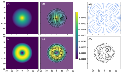
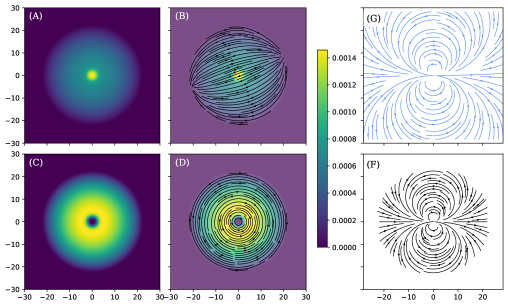
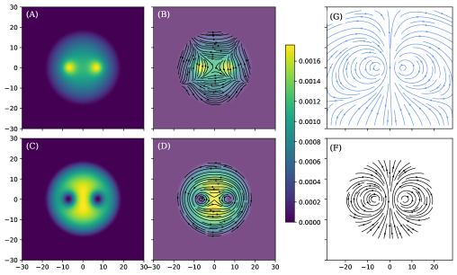
In the following gallery of figures we show the condensate superfluid density and velocity , for component , panels (A) and (B); and for component , panels (C) and (D), respectively. In panel (E), we show the Skyrmion spin texture and in panel (F) the transverse spin texture field lines . In panel (G) we show the transverse magnetic field lines that produces the corresponding condensate. Note that the transverse spin texture streamlines follow those of the transverse magnetic field. Details of the corresponding cases are given in the figures captions.
References
References
- Skyrme (1961) T. H. R. Skyrme, Proceedings of the Royal Society of London. Series A. Mathematical and Physical Sciences 260, 127 (1961), URL https://doi.org/10.1098/rspa.1961.0018.
- Adkins et al. (1983) G. S. Adkins, C. R. Nappi, and E. Witten, Nuclear Physics B 228, 552 (1983), URL https://www.sciencedirect.com/science/article/pii/055032138390559X.
- Meissner and Zahed (1986) U. Meissner and I. Zahed, Advances in Nuclear Physics 17:1 (1986), URL https://www.osti.gov/biblio/5329357.
- Holzwarth and Schwesinger (1986) G. Holzwarth and B. Schwesinger, Reports on Progress in Physics 49, 825 (1986), URL https://dx.doi.org/10.1088/0034-4885/49/8/001.
- Schwesinger et al. (1989) B. Schwesinger, H. Weigel, G. Holzwarth, and A. Hayashi, Physics Reports 173, 173 (1989), URL https://www.sciencedirect.com/science/article/pii/0370157389900227.
- Brey et al. (1995) L. Brey, H. A. Fertig, R. Côté, and A. H. MacDonald, Physical Review Letters 75, 2562 (1995), URL https://link.aps.org/doi/10.1103/PhysRevLett.75.2562.
- Rößler et al. (2006) U. K. Rößler, A. N. Bogdanov, and C. Pfleiderer, Nature 442, 797 (2006), URL https://doi.org/10.1038/nature05056.
- Hoffmann et al. (2017) M. Hoffmann, B. Zimmermann, G. P. Müller, D. Schürhoff, N. S. Kiselev, C. Melcher, and S. Blügel, Nature Communications 8, 308 (2017), URL https://doi.org/10.1038/s41467-017-00313-0.
- Romming et al. (2013) N. Romming, C. Hanneken, M. Menzel, J. E. Bickel, B. Wolter, K. von Bergmann, A. Kubetzka, and R. Wiesendanger, Science 341, 636 (2013), URL https://doi.org/10.1126/science.1240573.
- Dupé et al. (2014) B. Dupé, M. Hoffmann, C. Paillard, and S. Heinze, Nature Communications 5, 4030 (2014), URL https://doi.org/10.1038/ncomms5030.
- Leonov and Mostovoy (2015) A. O. Leonov and M. Mostovoy, Nature Communications 6, 8275 (2015), URL https://doi.org/10.1038/ncomms9275.
- Nagaosa and Tokura (2013) N. Nagaosa and Y. Tokura, Nature Nanotechnology 8, 899 (2013), URL https://doi.org/10.1038/nnano.2013.243.
- Jalil and Tan (2014) M. B. A. Jalil and S. G. Tan, Scientific Reports 4, 5123 (2014), URL https://doi.org/10.1038/srep05123.
- Wright and Mermin (1989) D. C. Wright and N. D. Mermin, Reviews of Modern Physics 61, 385 (1989), URL https://link.aps.org/doi/10.1103/RevModPhys.61.385.
- Leonov et al. (2014) A. O. Leonov, I. E. Dragunov, U. K. Rößler, and A. N. Bogdanov, Physical Review E 90, 042502 (2014), URL https://link.aps.org/doi/10.1103/PhysRevE.90.042502.
- Al Khawaja and Stoof (2001) U. Al Khawaja and H. Stoof, Nature 411, 918 (2001), URL https://doi.org/10.1038/35082010.
- Kasamatsu et al. (2005) K. Kasamatsu, M. Tsubota, and M. UEDA, International Journal of Modern Physics B 19, 1835 (2005), URL https://doi.org/10.1142/S0217979205029602.
- Leanhardt et al. (2003) A. E. Leanhardt, Y. Shin, D. Kielpinski, D. E. Pritchard, and W. Ketterle, Physical Review Letters 90, 140403 (2003), URL https://link.aps.org/doi/10.1103/PhysRevLett.90.140403.
- Pietilä and Möttönen (2009) V. Pietilä and M. Möttönen, Physical Review Letters 103, 030401 (2009), URL https://link.aps.org/doi/10.1103/PhysRevLett.103.030401.
- Leslie et al. (2009) L. S. Leslie, A. Hansen, K. C. Wright, B. M. Deutsch, and N. P. Bigelow, Physical Review Letters 103, 250401 (2009), URL https://link.aps.org/doi/10.1103/PhysRevLett.103.250401.
- Choi et al. (2012a) J.-y. Choi, W. J. Kwon, and Y.-i. Shin, Physical Review Letters 108, 035301 (2012a), URL https://link.aps.org/doi/10.1103/PhysRevLett.108.035301.
- Su et al. (2012) S. W. Su, I. K. Liu, Y. C. Tsai, W. M. Liu, and S. C. Gou, Physical Review A 86, 023601 (2012), URL https://link.aps.org/doi/10.1103/PhysRevA.86.023601.
- Xu and Han (2012) X.-Q. Xu and J. H. Han, Physical Review A 86, 063619 (2012), URL https://link.aps.org/doi/10.1103/PhysRevA.86.063619.
- LIU et al. (2013) Y.-K. LIU, C. ZHANG, and S.-J. YANG, Modern Physics Letters B 27, 1350183 (2013), URL https://doi.org/10.1142/S0217984913501832.
- Huang and Yip (2013) C.-C. Huang and S. K. Yip, Physical Review A 88, 013628 (2013), URL https://link.aps.org/doi/10.1103/PhysRevA.88.013628.
- Choi et al. (2012b) J.-y. Choi, W. J. Kwon, M. Lee, H. Jeong, K. An, and Y.-i. Shin, New Journal of Physics 14, 053013 (2012b), URL https://dx.doi.org/10.1088/1367-2630/14/5/053013.
- Hu et al. (2015) Y.-X. Hu, C. Miniatura, and B. Grémaud, Physical Review A 92, 033615 (2015), URL https://link.aps.org/doi/10.1103/PhysRevA.92.033615.
- Lovegrove et al. (2016) J. Lovegrove, M. O. Borgh, and J. Ruostekoski, Physical Review A 93, 033633 (2016), URL https://link.aps.org/doi/10.1103/PhysRevA.93.033633.
- Borgh et al. (2016) M. O. Borgh, M. Nitta, and J. Ruostekoski, Physical Review Letters 116, 085301 (2016), URL https://link.aps.org/doi/10.1103/PhysRevLett.116.085301.
- Dong et al. (2017) B. Dong, Q. Sun, W.-M. Liu, A.-C. Ji, X.-F. Zhang, and S.-G. Zhang, Physical Review A 96, 013619 (2017), URL https://link.aps.org/doi/10.1103/PhysRevA.96.013619.
- Zamora-Zamora and Romero-Rochín (2018) R. Zamora-Zamora and V. Romero-Rochín, Journal of Physics B: Atomic, Molecular and Optical Physics 51, 045301 (2018), URL https://dx.doi.org/10.1088/1361-6455/aaa324.
- Liu et al. (2024) Y.-K. Liu, N. Yue, J.-J. Zhang, and S.-J. Yang, Results in Physics 56, 107263 (2024), URL https://www.sciencedirect.com/science/article/pii/S2211379723010562.
- Marzlin et al. (2000) K.-P. Marzlin, W. Zhang, and B. C. Sanders, Physical Review A 62, 013602 (2000), URL https://link.aps.org/doi/10.1103/PhysRevA.62.013602.
- Ruostekoski and Anglin (2001) J. Ruostekoski and J. R. Anglin, Physical Review Letters 86, 3934 (2001), URL https://link.aps.org/doi/10.1103/PhysRevLett.86.3934.
- Battye et al. (2002) R. A. Battye, N. R. Cooper, and P. M. Sutcliffe, Physical Review Letters 88, 080401 (2002), URL https://link.aps.org/doi/10.1103/PhysRevLett.88.080401.
- Mizushima et al. (2002) T. Mizushima, K. Machida, and T. Kita, Physical Review Letters 89, 030401 (2002), URL https://link.aps.org/doi/10.1103/PhysRevLett.89.030401.
- Pietilä et al. (2007) V. Pietilä, M. Möttönen, and S. M. M. Virtanen, Physical Review A 76, 023610 (2007), URL https://link.aps.org/doi/10.1103/PhysRevA.76.023610.
- Kawakami et al. (2012) T. Kawakami, T. Mizushima, M. Nitta, and K. Machida, Physical Review Letters 109, 015301 (2012), URL https://link.aps.org/doi/10.1103/PhysRevLett.109.015301.
- Liu et al. (2013) Y.-K. Liu, C. Zhang, and S.-J. Yang, Physics Letters A 377, 3300 (2013), URL https://www.sciencedirect.com/science/article/pii/S037596011300978X.
- Luo et al. (2019) H.-B. Luo, L. Li, and W.-M. Liu, Scientific Reports 9, 18804 (2019), URL https://doi.org/10.1038/s41598-019-54856-x.
- Chen et al. (2022) Z. Chen, S. X. Hu, and N. P. Bigelow, Journal of Low Temperature Physics 208, 172 (2022), URL https://doi.org/10.1007/s10909-022-02724-w.
- Tiurev et al. (2018) K. Tiurev, T. Ollikainen, P. Kuopanportti, M. Nakahara, D. S. Hall, and M. Möttönen, New Journal of Physics 20, 055011 (2018), URL https://dx.doi.org/10.1088/1367-2630/aac2a8.
- Wilczek and Zee (1983) F. Wilczek and A. Zee, Physical Review Letters 51, 2250 (1983), URL https://link.aps.org/doi/10.1103/PhysRevLett.51.2250.
- Dzyaloshinsky (1958) I. Dzyaloshinsky, Journal of Physics and Chemistry of Solids 4, 241 (1958), URL https://www.sciencedirect.com/science/article/pii/0022369758900763.
- Moriya (1960) T. Moriya, Physical Review 120, 91 (1960), URL https://link.aps.org/doi/10.1103/PhysRev.120.91.
- Heinze et al. (2011) S. Heinze, K. von Bergmann, M. Menzel, J. Brede, A. Kubetzka, R. Wiesendanger, G. Bihlmayer, and S. Blügel, Nature Physics 7, 713 (2011), URL https://doi.org/10.1038/nphys2045.
- Shnir (2018) Y. M. Shnir, Topological and Non-Topological Solitons in Scalar Field Theories (Cambridge University Press, Cambridge, UK, 2018).
- Lin et al. (2009a) F. Lin, T. Lin, and W. J., Acta Mathematica Scientia 29B, 751 (2009a).
- Kawaguchi and Ueda (2012) Y. Kawaguchi and M. Ueda, Physics Reports 520, 253 (2012), URL https://www.sciencedirect.com/science/article/pii/S0370157312002098.
- Zamora-Zamora et al. (2012) R. Zamora-Zamora, M. Lozada-Hidalgo, S. F. Caballero-Benítez, and V. Romero-Rochín, Physical Review A 86, 053624 (2012), URL https://link.aps.org/doi/10.1103/PhysRevA.86.053624.
- Stamper-Kurn and Ueda (2013) D. M. Stamper-Kurn and M. Ueda, Reviews of Modern Physics 85, 1191 (2013), URL https://link.aps.org/doi/10.1103/RevModPhys.85.1191.
- Ueda (2014) M. Ueda, Reports on Progress in Physics 77, 122401 (2014), URL https://dx.doi.org/10.1088/0034-4885/77/12/122401.
- Weatherburn (1930) C. Weatherburn, Differential Geometry of Three Dimensions, vol. Volume II (Cambridge University Press, Cambridge, UK, 1930).
- Kreyszig (1991) E. Kreyszig, Differential Geometry (Dover Publications, Garden City, New York, 1991).
- McCleary (1997) J. McCleary, Geometry from a differentiable viewpoint (University Press, Cambridge, UK, 1997).
- do Carmo (2016) M. P. do Carmo, Differential Geometry of Curves and Surfaces (Dover Publications, Inc., Mineola, New York, 2016), second edition ed.
- Lin et al. (2009b) Y. J. Lin, R. L. Compton, K. Jiménez-García, J. V. Porto, and I. B. Spielman, Nature 462, 628 (2009b), URL https://doi.org/10.1038/nature08609.
- Dalibard et al. (2011) J. Dalibard, F. Gerbier, G. Juzeliūnas, and P. Öhberg, Reviews of Modern Physics 83, 1523 (2011), URL https://link.aps.org/doi/10.1103/RevModPhys.83.1523.
- Berry (1984) M. Berry, Proceedings of the Royal Society of London. Series A. Mathematical and Physical Sciences 392, 45 (1984).
- Schwarz (1994) A. S. Schwarz, Topology for Physicists (Springer-Verlag, Berlin, Germany, 1994).
- Mermin (1979) N. D. Mermin, Reviews of Modern Physics 51, 591 (1979), URL https://link.aps.org/doi/10.1103/RevModPhys.51.591.
- Zeng and Zhang (2009) R. Zeng and Y. Zhang, Computer Physics Communications 180, 854 (2009), URL https://www.sciencedirect.com/science/article/pii/S0010465508004207.