A Sampling-based Progressive Hedging Algorithm for Stochastic Programming

Abstract

The progressive hedging algorithm (PHA) is a cornerstone among algorithms for large-scale stochastic programming problems. However, its traditional implementation is hindered by some limitations, including the requirement to solve all scenario subproblems in each iteration, reliance on an explicit probability distribution, and a convergence process that is highly sensitive to the choice of certain penalty parameters. This paper introduces a sampling-based PHA which aims to overcome these limitations. Our approach employs a dynamic selection process for the number of scenario subproblems solved per iteration. It incorporates adaptive sequential sampling for determining sample sizes, a stochastic conjugate subgradient method for direction finding, and a line-search technique to update the dual variables. Experimental results demonstrate that this novel algorithm not only addresses the bottlenecks of the conventional PHA but also potentially surpasses its scalability, representing a substantial improvement in the field of stochastic programming.

1 Introduction

1.1 Problem setup

In this paper, we focus on a task of solving a Stochastic Programming (SP) stated as follows.

$$\min_{x\in X\subseteq\mathbb{R}^{n}}f(x)=E_{\tilde{\omega}}[h(x,\tilde{\omega})],$$ (1)

where $\tilde{\omega}\in\mathbb{R}^{m}$ denotes a random vector and $h(\cdot,\tilde{\omega})$ is a finite valued convex function in $x$ for any particular realization $\tilde{\omega}=\omega$. Except in very simplistic situations (e.g., when $\tilde{\omega}$ has a small number of outcomes), solving the optimization problem (1) using deterministic algorithms is infeasible. To overcome challenges arising from efforts to solve realistic instances, the focus often shifts towards solving a sample average approximation (SAA) problem. In such an approach, we create an approximation by using $|S|$ i.i.d. realizations of $\tilde{\omega}$ called scenarios, and denote them by $\omega^{1},...,\omega^{|S|}$. In this setting, (1) can be reformulated as

$$\min_{x\in X}f(x)=\frac{1}{|S|}\sum_{s=1}^{|S|}h(x,\omega^{s}),$$ (2)

In order to establish an optimal solution of (2), many algorithms have been proposed and one of the more popular algorithms among them is the progressive hedging (PH) algorithm [20]. To lay the groundwork, we will commence by reviewing the classic PH algorithm.

1.2 Classic Progressive Hedging Algorithm

The PH Algorithm is a version of alternating direction method of multipliers (ADMM) [6] which has attracted significant attention in stochastic programming community, extensively utilized for addressing scenario-based uncertainty in large-scale optimization problems. Originally conceptualized by Rockafellar and Wets in 1991 [20], the algorithm has evolved significantly, finding applications in diverse fields such as finance, energy, and logistics [25]. The convergence properties of the PH algorithm have been rigorously analyzed since its inception. Rockafellar and Wets provided the initial proof of convergence for convex problems. Further research, such as that by Ruszczyński and Shapiro [21], explored the conditions under which PH algorithm converges, including scenarios involving non-convexities and other complexities. However, despite its wide-spread popularity, classic PH algorithm remains a deterministic algorithm which immediately hinders its applicability for broader stochastic optimization problems. For instance, in applications where the uncertainty can only be sampled via simulation or the sample space is so vast that it is unrealistic to expect a knowledge of all possible outcomes associated with the data. More specifically, the limitations include

• First, in contrast to several SP algorithms, notably stochastic gradient descent (SGD), classic PH algorithm necessitates the resolution of all subproblems during each iteration. This requirement constitutes a significant computational bottleneck, substantially impeding its scalability and performance.

• Second, the convergence criteria of the PH algorithm are predicated upon the accessibility and knowledge of the probability distribution of the random variables involved. This requirement severely restricts the algorithm’s utility in situations where such a distribution remains unknown or is difficult to ascertain, thereby restricting its range of applications.

• Lastly, the algorithm employs a dual update rule which is fundamentally gradient-based and is accurate solely at the current dual point. Also, this approach renders the convergence process highly dependent on the appropriate selection of the penalty parameter which acts as a step size in the dual update. The performance of the algorithm, therefore, hinges on the specification of the subgradient and the penalty parameter, further complicating its practical performance.

For instances which present such challenges, an adaptive sampling algorithm maybe more suitable because such methods allow a possibility of creating approximations which are able to sequentially adapt to the data which is revealed during the course of the algorithm. In this paper, we will introduce an innovative sampling-based PH algorithm which adaptively samples a subset of scenario subproblems in each iteration, facilitating dynamic scenario updates to enhance computational efficiency.

1.3 Adaptive sampling

Classic PH algorithm relies on the knowledge of the probability distribution of the random variables. When the probability distribution is not available, the PH algorithm typically employs sample average approximation (SAA) [23] which has a fixed sample size to estimate these uncertainties. However, it is difficult to determine the sample size [22, 9] when applying such method to the PH algorithm and convergence properties have only been established for cases with only a finite number of outcomes. While adaptive sampling [14] has emerged as a powerful approach for instances with a large number of outcomes (especially for multi-dimensional uncertainty), such adaptive sampling has remained elsuive in the context of PH. Adaptive sampling dynamically adjusts the sample size based on ongoing optimization progress, providing a more resource-efficient and precise solution. Some effort has been made to combine adaptive sampling with PH algorithm. For instance, [3] provides randomized PH methods which is able to produce new iterates as soon as a single scenario subproblem is solved. [1] proposes a SBPHA approach which is a combination of replication and PH algorithm. However, these methods, although provide a ”randomized” PH algorithm, still sample a subset of scenarios from a fixed finite collection in each iteration, without dynamically determining the sample size based on the optimization procedure. On the other hand, our sampling-based PH algorithm will strategically sample a subset of scenario subproblems in each iteration, facilitating dynamic scenario updates to enhance computational efficiency. We will also leverage the sample complexity analysis [24] to support the choice of the sample size, ensuring a theoretically grounded approach.

1.4 Stochastic conjugate gradient method

The dual update of classic PH algorithm can be considered as a stochastic first-order (SFO) method [19, 5]. First-order gradient-based methods dominate the field for several convincing reasons: low computational cost, simplicity of implementation, and strong empirical results. However SFO methods are not known for their numerical accuracy especially when the functions are non-smooth and the classic convergence rate [16] only applies under the assumption that the component functions are smooth.

In contrast to first-order methods, algorithms based on conjugate gradients (CG) provide finite termination when the objective function is a linear-quadratic deterministic function [17]. Furthermore, CG algorithms are also used for large-scale nonsmooth convex optimization problems [27, 29]. However, despite its many strengths, (e.g., fast per-iteration convergence, frequent explicit regularization on step-size, and better parallelization than first-order methods), the use of conjugate gradient methods for SP is uncommon. Although [13, 28] proposed some new stochastic conjugate gradient (SCG) algorithms, their assumptions do not support non-smooth objective functions, and hence not directly applicable to our problems.

In order to solve stochastic optimization problems when functions are non-smooth (as in (2)), it is straightforward to imagine that a stochastic subgradient method could be used. In this paper, we treat the dual optimization problem in PH as a stochastic linear quadratic optimization problem and propose to leverage a stochastic conjugate subgradient (SCS) direction originated from [26, 27] which accommodates both the curvature of a quadratic function, as well as the decomposition of subgradients by data points, as is common in stochastic programming [11, 12]. This combination enhances the power of stochastic first-order approaches without the additional burden of second-order approximations. In other words, our method shares the spirit of Hessian Free (HF) optimization, which has attracted some attention in the machine learning community [15, 8]. As our theoretical analysis and the computational results reveal, the new method provides a “sweet-spot” at the intersection of speed, accuracy, and scalability of algorithms (see Theorems 3.12 and 3.14).

1.5 Penalty parameter and line-search algorithm

In the original Progressive Hedging (PH) algorithm, Rockafellar and Wets briefly discussed the effect of the penalty parameter on the performance of the PH algorithm and the quality of the solution, but they did not provide any guidance on how to choose it. Various choices have since been proposed, often differing with the application under consideration. Readers interested in the selection of the penalty parameter can refer to [30], which offers a comprehensive literature review of related methods.

Our approach differs from these methods by employing a stochastic direction-finding technique [18, 2] derived from Wolfe’s line-search method [26, 27]. Compared with existing approaches, our method is more mathematically motivated and adheres to the principles of optimization [7].

2 Sampling-based Progressive Hedging Algorithm

In this section, we focus on solving (1) using the a sampling-based PHA in which we combine classic PHA[20] with adaptive sampling in stochastic programming [4]. The main ingredients of the algorithm include six important components:

• Sequential scenarios sampling. At iteration $k$, different from classic PH Algorithm which solves all scenarios subproblems, we will sample $|S_{k}|$ scenarios and only solve the subproblelms corresponding to these scenarios. It is similar as using sample average approximation (SAA) to approximate function $f$ using $f_{k}$,

  $$f_{k}(x)=\frac{1}{|S_{k}|}\sum_{s=1}^{|S_{k}|}h(x,\omega^{s}),$$ (3)

  where $|S_{k}|$ will be determined based on concentration inequalities in Theorem 3.5.

• Update the primal variables. In each scenarios $s\in S_{k}$, similar to the classic PHA, we will first solve the corresponding augmented Lagrangian problem

  $$x_{k}^{s}=\operatorname*{arg\,min}_{x^{s}\in X}h(x^{s},\omega^{s})+\langle\lambda_{k}^{s},x^{s}-\bar{x}_{k-1}\rangle+\frac{\rho}{2}||x^{s}-x_{k-1}||^{2}.$$ (4)

  Then a feasible solution will be

  $$\bar{x}_{k}=\frac{1}{|S_{k}|}\sum_{s=1}^{|S_{k}|}x_{k}^{s}.$$ (5)

• Conjugate subgradient direction finding. The idea here is inspired by Wolfe’s non-smooth conjugate subgradient method which uses the smallest norm of the convex combination of the previous search direction $d_{k-1}^{s}$ and the current subgradient $g_{k}^{s}=x_{k}^{s}-\bar{x}_{k}$. More specifically, we first solve the following one-dimensional QP

  $$\gamma_{k}^{s}=\operatorname*{arg\,min}_{\gamma^{s}\in[0,1]}\frac{1}{2}||\gamma^{s}d_{k-1}^{s}+(1-\gamma^{s})g_{k}^{s}||^{2}.$$ (6)

  Then we can set the new direction

  $$d_{k}^{s}=\gamma_{k}^{s}d_{k-1}^{s}+(1-\gamma_{k}^{s})g_{k}^{s}:=Nr(G_{k}^{s}),$$

  where $G_{k}^{s}=\{g_{k}^{s},d_{k-1}^{s}\}$.

• Update the dual variables using line-search. We will update $\hat{\lambda}_{k+1}^{s}=\lambda_{k}^{s}+\theta_{k}^{s}d_{k}^{s}$. Define

  $$L_{k}^{s}(\lambda_{k}^{s}+\theta^{s}d_{k}^{s}):=h(\hat{x}_{k}^{s},\omega^{s})+\langle\lambda_{k}^{s}+\theta^{s}d_{k}^{s},\hat{x}_{k}^{s}-\hat{x}_{k}\rangle+\frac{\rho}{2}||\hat{x}_{k}^{s}-\hat{x}_{k}||^{2},$$ (7)

  where $\delta_{k}^{s}$ is the stochastic searching region, $\hat{x}_{k}^{s}$ and $\hat{x}_{k}$ are obtained by replacing $\lambda_{k}^{s}$ in (4) with $\lambda_{k}^{s}+\theta d_{k}^{s}$ in each scenario and resolving (4) and (5), respectively. The step size $\theta_{k}^{s}$ will be obtained by performing an inexact line-search which makes it satisfy the strong-Wolfe condition [26, 27]. Let $g^{s}(\theta^{s})\in\partial_{\lambda^{s}}L_{k}^{s}(\lambda_{k}^{s}+\theta^{s}\cdot d_{k}^{s})$ and define the intervals $L$ and $R$.

  $$L=\{\theta^{s}>0\ |\ L_{k}^{s}(\lambda_{k}+\theta^{s}\cdot d_{k})-L_{k}^{s}(\lambda_{k})\geq m_{1}||d_{k}^{s}||^{2}\theta^{s}\},$$ (8)

  $$R=\{\theta^{s}>0\ |\ \sum_{s=1}^{S_{k}}\langle g^{s}(\theta^{s}),d_{k}^{s}\rangle\leq m_{2}||d_{k}^{s}||^{2}\},$$

  where $m_{2}<m_{1}<1/2$. The output of the step size will satisfy two metrics: (i) Identify a set $L$ which includes points which sufficiently increase the dual objective function approximation $L_{k}^{s}$, and (ii) Identify a set $R$ for which the directional derivative estimate for $L_{k}^{s}$ is sufficiently decreased. The algorithm seeks points which belong to $L\cap R$. The combination of $L$ and $R$ is called strong-Wolfe condition and it has been shown in [27] (Lemma 1) that $L\cap R$ is not empty.

  Intuitively, the above procedure is a line-search along conjugate direction $d_{k}^{s}$ and the goal is to (approximately) maximize the dual objective function $L_{k}^{s}$.

• Stochastic searching region update. Similar to the standard stochastic trust region method [2], let $\gamma>1$, $\eta\in(0,1)$, $\lambda_{k}:=(\lambda_{k}^{1},...,\lambda_{k}^{|S_{k}|})$ and $L_{k}(\lambda_{k}):=\sum_{s=1}^{|S_{k}|}L_{k}^{s}(\lambda_{k}^{s})$, if

  $$L_{k}(\hat{\lambda}_{k})-L_{k}(\lambda_{k-1})>\eta[L_{k-1}(\hat{\lambda}_{k})-L_{k-1}(\lambda_{k-1})],$$ (9)

  set $\delta_{k}=\gamma\delta_{k-1}$ and $\lambda_{k}=\hat{\lambda}_{k}$. Otherwise, set $\delta_{k}=\delta_{k-1}/\gamma$ and $\lambda_{k}=\lambda_{k-1}$.

• Termination criteria. Define $d_{k}:=(d_{k}^{1},...,d_{k}^{|S_{k}|})$ and $||d_{k}||:=\frac{1}{|S_{k}|}\sum_{s=1}^{|S_{k}|}||d_{k}^{s}||$. The algorithm concludes its process when $||d_{k}||<\varepsilon$ and $\delta_{k}<\delta_{min}$. As we will show in Theorem 3.14, a dimunitive value of $||d_{k}||$ indicates a small norm of the gradient $g_{k}$, fulfilling the optimality condition for an unconstrained convex optimization problem. Additionally, a threshold $\delta_{min}$ is established to prevent premature termination in the initial iterations. Without this threshold, the algorithm may halt prematurely if the initial samples are correctly classified by the initial classifier $\alpha_{0}$, resulting in $||d_{k}||<\varepsilon$. However, if $\delta_{min}$ is introduced, based on Theorem 3.5, $|S_{k}|$ should be chosen such that

  $$|S_{k}|\geq-8\log(\varepsilon/2)\cdot\frac{M_{1}^{2}}{\kappa^{2}\delta_{k}^{4}},$$

  where $\kappa$ is the $\kappa$-approximation defined in Definition 3.2. This effectively mitigates any early stopping concern with high probability.

Initialize $\bar{x}_{0}\in W$, $\lambda_{0}=(\lambda_{0}^{1},...,\lambda_{0}^{|S_{0}|})=\vv{0}$, $d_{0}=(d_{0}^{1},d_{0}^{2},...,d_{0}^{|S_{0}|})$, $\rho>0$, , $\gamma>1$, $\eta\in(0,1)$, $\delta_{0}\in[\delta_{min},\delta_{max}]$ and $\varepsilon>0$.

while $||d_{k}||>\varepsilon$ do

      

      Randomly draw a scenarios set with $S_{k}$ scenarios.

      $x_{k}^{s}=\operatorname*{arg\,min}_{x^{s}\in X}h(x^{s},\omega^{s})+\lambda_{k}^{s}(x^{s}-\bar{x}_{k-1})+\frac{\rho}{2}||x^{s}-\bar{x}_{k-1}||^{2}$, $\forall s$.

      $\bar{x}_{k}=\frac{1}{S_{k}}\sum_{s=1}^{S}x_{k}^{s}$.

      Calculate $g_{k}^{s}=x_{k}^{s}-x_{k}$, $G_{k}^{s}=\{d_{k-1}^{s},g_{k}^{s}\}$ and $d_{k}^{s}=Nr(G_{k})$, $\forall s$.

      Apply line-search algorithm to find a step size $\theta_{k}^{s}$ which belongs to $L\cap R$.

      Update $\hat{\lambda}_{k}^{s}=\lambda_{k-1}^{s}+\theta_{k}^{s}d_{k}^{s}$, $\forall s$.

      if (9) is satisfied then

             $\lambda_{k}\leftarrow\hat{\lambda}_{k},\quad\delta_{k}\leftarrow\min\{\gamma\delta_{k-1},\delta_{max}\}$;

            

      else

             $\lambda_{k}\leftarrow\lambda_{k-1},\quad\delta_{k}\leftarrow\max\{\frac{\delta_{k-1}}{\gamma},\delta_{min}\}$;

            

       end if

      

end while

Algorithm 1 Sampling-based Progressive Hedging Algorithm

3 Convergence Properties

3.1 Scenario Dual Objective Functions

Definition 3.1.

For any $\omega^{s}$, $\bar{x}$ and $\lambda^{s}$, define the scenario optimal solution

$$x^{s}(\lambda^{s},\omega^{s})=\operatorname*{arg\,min}_{x\in X}h(x,\omega^{s})+\langle\lambda^{s},x-\bar{x}\rangle,$$

and the corresponding scenario dual objective function

$$L^{s}(\lambda^{s};w^{s},\bar{x})=h(x^{s},\omega^{s})+\langle\lambda^{s},x^{s}-\bar{x}\rangle.$$

Lemma 3.1.

In any iteration of Algorithm 1, we have $\sum_{s=1}^{|S_{k}|}\lambda_{k}^{s}=0$.

Proof.

We will show the lemma by induction. When $k=0$, $\lambda_{0}^{s}=0$, for all $s\in S_{0}$. Thus, the statement is correct. Next, when $k=1$, we have

$$\lambda_{1}^{s}=\rho(x_{1}^{s}-\bar{x}_{k})=\rho(x_{1}^{s}-\frac{1}{|S_{1}|}\sum_{s=1}^{|S_{1}|}x_{1}^{s}),$$

then

$$\sum_{s=1}^{|S_{1}|}\lambda_{1}^{s}=\rho\sum_{s=1}^{|S_{1}|}(x_{1}^{s}-\frac{1}{|S_{1}|}\sum_{s=1}^{|S_{1}|}x_{1}^{s})=0.$$

Suppose it is true for $k=n$, i.e., $\sum_{s=1}^{|S_{n}|}\lambda_{n}^{s}=0$, then for $k=n+1$,

$$\sum_{s=1}^{|S_{n+1}|}\lambda_{n+1}^{s}=\sum_{s=1}^{|S_{n}|}\lambda_{n}^{s}+\rho\sum_{s=1}^{|S_{n+1}|}(x_{n+1}^{s}-\bar{x}_{n+1})=0,$$

where the first part is $0$ by the induction hypothesis and the second part is $0$ by the construction of Algorithm 1. We thus conclude the proof.

∎

Theorem 3.2.

In every iteration of Algorithm 1, we have

$$\frac{1}{|S_{k}|}\sum_{s=1}^{|S_{k}|}L_{k}^{s}(\lambda_{k}^{s};\omega^{s},\bar{x}_{k})=\frac{1}{|S_{k}|}\sum_{s=1}^{|S_{k}|}L_{k}^{s}(\lambda_{k}^{s};\omega^{s}):=\frac{1}{|S_{k}|}\sum_{s=1}^{|S_{k}|}h(x_{k}^{s},\omega^{s})+\langle\lambda_{k}^{s},x_{k}^{s}\rangle.$$

Proof.

$$\frac{1}{|S_{k}|}\sum_{s=1}^{|S_{k}|}L^{s}(\lambda^{s};\omega^{s},\bar{x}_{k})=\frac{1}{|S_{k}|}\sum_{s=1}^{|S_{k}|}[h(x_{k}^{s},\omega^{s})+\langle\lambda_{k}^{s},x_{k}^{s}\rangle]+\frac{1}{|S_{k}|}\sum_{s=1}^{|S_{k}|}\langle\lambda_{k}^{s},\bar{x}_{k}\rangle,$$

where the last part is $0$ by Lemma 3.1. ∎

3.2 Stochastic Local Approximation

Assumption 1.

The primal feasible region $X$ is bounded, i.e., there exists a constant $C$ such that for any $x\in X$, we have $||x||\leq C$.

Assumption 2.

For any $\omega^{s}$ and $\lambda^{s}$, $L^{s}(\lambda^{s};\omega^{s})$ is bounded, i.e., there exists a constant $M$, such that $|L^{s}(\lambda^{s};\omega^{s})|\leq M$.

Assumption 3.

For any $\omega^{s}$, $L^{s}(\lambda^{s};\omega^{s})$ possesses a Lipschitz constant $0<L<\infty$ and the sub-differentials are non-empty for every $\lambda^{s}$.

Assumption 4.

For any $\omega^{s}$ and $\lambda^{s}$, $L^{s}(\lambda^{s};\omega^{s})$ has bounded sub-differential set, i.e., for any $g^{s}\in\partial_{\lambda^{s}}L^{s}(\lambda^{s};\omega^{s})$, we have $||g^{s}||\leq G$.

Definition 3.2.

A multi-variable function $L_{k}(\lambda^{1},...,\lambda^{|S|})$ is a local $\kappa$-approximation of $L(\lambda^{1},...,\lambda^{|S|})$ on $\mathcal{B}(\lambda_{k}^{s},\delta_{k})$, if for all $\lambda^{s}\in\mathcal{B}(\lambda_{k}^{s},\delta_{k})$,

$$|L(\lambda^{1},...,\lambda^{|S|})-L_{k}(\lambda^{1},...,\lambda^{|S|})|\leq\kappa\delta_{k}^{2}.$$

Definition 3.3.

Let $\Delta_{k}$, $\Lambda_{k}^{s}$ denote the random counterpart of $\delta_{k}$, $\lambda_{k}^{s}$, respectively, and $\mathcal{L}_{k}$ denote the $\sigma$-algebra generated by $\{\mathcal{L}_{i}\}_{i=0}^{k-1}$. A sequence of random models $\{\mathcal{L}_{k}\}$ is said to be $\mu_{1}$-probabilistically $\kappa$-approximation of $\mathcal{L}$ with respect to $\{\mathcal{B}(\Lambda_{k}^{s},\Delta_{k})\}$ if the event

$$I_{k}\overset{\Delta}{=}\{\mathcal{L}_{k}\ \textit{is}\ \kappa-\textit{approximation of}\ \mathcal{L}\ \textit{on}\ \mathcal{B}(\Lambda_{k}^{s},\Delta_{k})\}$$

satisfies the condition

$$\mathbb{P}(I_{k}|\mathcal{L}_{k-1})\geq\mu_{1}>0.$$

Lemma 3.3.

If one added scenario $s_{i}\in S_{k}/S_{k-1}$ changes from $s_{i}$ to $s_{i}^{\prime}$, then for $s\in S_{k}/s_{i}$, we have

$$||g_{k}^{s}-(g_{k}^{s})^{\prime}||=O(\frac{1}{|S_{k}|}),\ |\gamma_{k}^{s}-(\gamma_{k}^{s})^{\prime}|=O(\frac{1}{|S_{k}|}),\ \textit{and}\ ||d_{k}^{s}-(d_{k}^{s})^{\prime}||=O(\frac{1}{|S_{k}|}).$$

Proof.

First, note that for $s\in S_{k}/s_{i}$,

$$g_{k}^{s}=x_{k}^{s}-\bar{x}_{k}=x_{k}^{s}-\frac{x_{k}^{1}+...+x_{k}^{s}+...+x_{k}^{|S_{k}|}}{|S_{k}|},$$

$$(g_{k}^{s})^{\prime}=x_{k}^{s}-\bar{x}_{k}^{\prime}=x_{k}^{s}-\frac{x_{k}^{1}+...+x_{k}^{s^{\prime}}+...+x_{k}^{|S_{k}|}}{|S_{k}|}.$$

Thus, by Assumption 1,

$$||g_{k}^{s}-(g_{k}^{s})^{\prime}||=\frac{||x_{k}^{s}-x_{k}^{s^{\prime}}||}{|S_{k}|}\leq\frac{2C}{|S_{k}|}.$$ (10)

Also, note that

$$\gamma_{k}^{s}=\operatorname*{arg\,min}_{\gamma^{s}\in[0,1]}||\gamma^{s}d_{k-1}^{s}+(1-\gamma^{s})g_{k}^{s}||^{2}=\frac{\langle d_{k-1}^{s},d_{k-1}^{s}-g_{k}^{s}\rangle}{||d_{k-1}^{s}-g_{k}^{s}||^{2}},$$

$$(\gamma_{k}^{s})^{\prime}=\operatorname*{arg\,min}_{\gamma^{s}\in[0,1]}||\gamma^{s}d_{k-1}^{s}+(1-\gamma^{s})(g_{k}^{s})^{\prime}||^{2}=\frac{\langle d_{k-1}^{s},d_{k-1}^{s}-(g_{k}^{s})^{\prime}\rangle}{||d_{k-1}^{s}-(g_{k}^{s})^{\prime}||^{2}}.$$

Let $\Delta g_{k}^{s}=(g_{k}^{s})^{\prime}-g_{k}^{s}$, we have

$$\gamma_{k}^{s}-(\gamma_{k}^{s})^{\prime} =\frac{\langle d_{k-1}^{s},d_{k-1}^{s}-g_{k}^{s}\rangle\cdot||d_{k-1}^{s}-g_{k}^{s}-\Delta g_{k}^{s}||^{2}}{||d_{k-1}^{s}-g_{k}^{s}||^{2}\cdot||d_{k-1}^{s}-g_{k}^{s}-\Delta g_{k}^{s}||^{2}}$$

$$-\frac{\langle d_{k-1}^{s},d_{k-1}^{s}-g_{k}^{s}-\Delta g_{k}^{s}\rangle\cdot||d_{k-1}^{s}-g_{k}^{s}||^{2}}{||d_{k-1}^{s}-g_{k}^{s}||^{2}\cdot||d_{k-1}^{s}-g_{k}^{s}-\Delta g_{k}^{s}||^{2}}$$

$$=\frac{\langle\Delta g_{k}^{s},d_{k-1}^{s}-g_{k}^{s}\rangle\cdot\langle d_{k-1}^{s},d_{k-1}^{s}-g_{k}^{s}\rangle}{||d_{k-1}^{s}-g_{k}^{s}||^{2}\cdot||d_{k-1}^{s}-g_{k}^{s}-\Delta g_{k}^{s}||^{2}}$$

$$+\frac{||\Delta g_{k}^{s}||^{2}\cdot\langle d_{k-1}^{s},d_{k-1}^{s}-g_{k}^{s}\rangle-\langle\Delta g_{k}^{s},d_{k-1}^{s}\rangle\cdot||d_{k-1}^{s}-g_{k}^{s}||^{2}}{||d_{k-1}^{s}-g_{k}^{s}||^{2}\cdot||d_{k-1}^{s}-g_{k}^{s}-\Delta g_{k}^{s}||^{2}}.$$

With Assumption 4, Eq. (10) and triangular inequality, we have

$$|\gamma_{k}^{s}-(\gamma_{k}^{s})^{\prime}|=O(\frac{1}{|S_{k}|})$$ (11)

Finally, to bound $||d_{k}^{s}-(d_{k}^{s})^{\prime}||$, note that

$$d_{k}^{s}=\gamma_{k}^{s}g_{k}^{s}+(1-\gamma_{k}^{s})d_{k-1}^{s},$$ (12)

$$(d_{k}^{s})^{\prime}=(\gamma_{k}^{s})^{\prime}(g_{k}^{s})^{\prime}+(1-(\gamma_{k}^{s})^{\prime})d_{k-1}^{s}.$$

Let $\Delta\gamma_{k}^{s}=(\gamma_{k}^{s})^{\prime}-\gamma_{k}^{s}$, then

$$d_{k}^{s}-(d_{k}^{s})^{\prime} =\gamma_{k}^{s}g_{k}^{s}+(1-\gamma_{k}^{s})d_{k-1}^{s}$$ (13)

$$-(\gamma_{k}^{s}+\Delta\gamma_{k}^{s})(g_{k}^{s}+\Delta g_{k}^{s})-(1-\gamma_{k}^{s}-\Delta\gamma_{k}^{s})d_{k-1}^{s}$$

$$=-\gamma_{k}^{s}\Delta g_{k}^{s}-\Delta\gamma_{k}^{s}g_{k}^{s}-\Delta\gamma_{k}^{s}\Delta g_{k}^{s}+\Delta\gamma_{k}^{s}d_{k-1}^{s}.$$

With Assumption 4, Eq. (10) and Eq. (11), we have

$$||d_{k}^{s}-(d_{k}^{s})^{\prime}||=O(\frac{1}{|S_{k}|}).$$ (14)

∎

Lemma 3.4.

If one added scenario $s_{i}\in S_{k}/S_{k-1}$ changes from $s_{i}$ to $s_{i}^{\prime}$, then for $s\in S_{k}/s_{i}$, we have

$$||x_{k}^{s}(\theta^{s})-(x_{k}^{s})^{\prime}(\theta^{s})||=O(\frac{1}{|S_{k}|}),\ \textit{and}$$

$$||L_{k}^{s}(\lambda_{k}^{s}+\theta_{k}^{s}d_{k}^{s};\omega^{s})-L_{k}^{s}(\lambda_{k}^{s}+(\theta_{k}^{s})^{\prime}(d_{k}^{s})^{\prime};\omega^{s})||=O(\frac{1}{|S_{k}|}).$$

Proof.

For any $\theta^{s}$, we have

$$x_{k}^{s}(\theta^{s})=\operatorname*{arg\,min}_{x^{s}\in X}h(x^{s},\omega^{s})+\langle\lambda_{k}^{s}+\theta^{s}d_{k}^{s},x^{s}-\bar{x}_{k}\rangle.$$

$$(x_{k}^{s})^{\prime}(\theta^{s})=\operatorname*{arg\,min}_{x^{s}\in X}h(x^{s},\omega^{s})+\langle\lambda_{k}^{s}+\theta^{s}(d_{k}^{s}+\Delta d_{k}^{s}),x^{s}-\bar{x}_{k}^{\prime}\rangle.$$

Note that we have only changed the objective coefficient of $x^{s}$ and the difference is $\theta^{s}\cdot\Delta d_{k}^{s}$. According to the sensitivity analysis in linear programming, $||\Delta d_{k}^{s}||=O(\frac{1}{|S_{k}|})$ and $\theta^{s}\in[\delta_{min},\delta_{max}]$, we have

$$||x_{k}^{s}(\theta^{s})-(x_{k}^{s})^{\prime}(\theta^{s})||=O(\theta^{s}\cdot||\Delta d_{k}^{s}||)=O(\frac{1}{|S_{k}|}).$$ (15)

Also, for any $\theta^{s}$, consider

$$g(\theta^{s};\omega^{s}):=h(x_{k}^{s}(\theta^{s}),\omega^{s})+\langle\lambda_{k}^{s}+\theta^{s}d_{k}^{s},x_{k}^{s}(\theta^{s})-\bar{x}_{k}\rangle.$$

$$g^{\prime}(\theta^{s};\omega^{s}):=h((x_{k}^{s})^{\prime}(\theta^{s}),\omega^{s})+\langle\lambda_{k}^{s}+\theta^{s}(d_{k}^{s})^{\prime},(x_{k}^{s})^{\prime}(\theta^{s})-\bar{x}_{k}^{\prime}\rangle.$$

Let $\Delta x_{k}^{s}(\theta^{s})=x_{k}^{s}(\theta^{s})-(x_{k}^{s})^{\prime}(\theta^{s})$ and $\Delta\bar{x}_{k}=\bar{x}_{k}^{\prime}-\bar{x}_{k}$, then we have

$$g(\theta^{s};\omega^{s})-g^{\prime}(\theta^{s};\omega^{s}) =h(x_{k}^{s}(\theta^{s}),\omega^{s})+\langle\lambda_{k}^{s}+\theta^{s}d_{k}^{s},x_{k}^{s}(\theta^{s})-\bar{x}_{k}\rangle$$

$$-(h((x_{k}^{s})^{\prime}(\theta^{s}),\omega^{s})+\langle\lambda_{k}^{s}+\theta^{s}(d_{k}^{s})^{\prime},(x_{k}^{s})^{\prime}(\theta^{s})-\bar{x}_{k}^{\prime}\rangle)$$

$$=h(x_{k}^{s}(\theta^{s}),\omega^{s})-h(x_{k}^{s}(\theta^{s})+\Delta x_{k}^{s}(\theta^{s});\omega^{s})$$

$$+\langle\lambda_{k}^{s}+\theta^{s}d_{k}^{s},x_{k}^{s}(\theta^{s})-\bar{x}_{k}\rangle$$

$$-\langle\lambda_{k}^{s}+\theta^{s}(d_{k}^{s}+\Delta d_{k}^{s}),x_{k}^{s}(\theta^{s})+\Delta x_{k}^{s}(\theta^{s})-\bar{x}_{k}+\Delta\bar{x}_{k}\rangle)$$

$$=h(x_{k}^{s}(\theta^{s}),\omega^{s})-h(x_{k}^{s}(\theta^{s})+\Delta x_{k}^{s}(\theta^{s});\omega^{s})$$

$$-\langle\lambda_{k}^{s},\Delta x_{k}^{s}(\theta^{s})\rangle+\langle\lambda_{k}^{s},\Delta\bar{x}_{k}\rangle-\langle\theta^{s}d_{k}^{s},\Delta x_{k}^{s}(\theta^{s})\rangle+\langle\theta^{s}d_{k}^{s},\Delta\bar{x}_{k}\rangle$$

$$-\langle\theta^{s}\Delta d_{k}^{s},x_{k}^{s}(\theta^{s})+\Delta x_{k}^{s}(\theta^{s})-\bar{x}_{k}+\Delta\bar{x}_{k}\rangle$$

With Assumption 3, Lemma 3.3 and Eq. (15), we have

$$||g(\theta^{s};\omega^{s})-g^{\prime}(\theta^{s};\omega^{s})||=O(\frac{1}{|S_{k}|}).$$ (16)

Since Eq. (16) is true for any $\theta^{s}$, we have

$$\ ||L_{k}^{s}(\lambda_{k}^{s}+\theta_{k}^{s}d_{k}^{s};\omega^{s})-L_{k}^{s}(\lambda_{k}^{s}+(\theta_{k}^{s})^{\prime}(d_{k}^{s})^{\prime};\omega^{s})||$$

$$= \ ||\max_{\theta^{s}}g(\theta^{s};\omega^{s})-\max_{\theta^{s}}g^{\prime}(\theta^{s};\omega^{s})||$$

$$\leq \ \max_{\theta^{s}}||g(\theta^{s};\omega^{s})-g^{\prime}(\theta^{s};\omega^{s})||$$

$$= \ O(\frac{1}{|S_{k}|}).$$

∎

Theorem 3.5.

Let $L(\lambda^{1},...,\lambda^{|S_{k}|}):=E_{\{\omega^{1},...,\omega^{s}\}}[\frac{1}{|S_{k}|}\sum_{s=1}^{|S_{k}|}L_{k}^{s}(\lambda^{s};\omega^{s})]$ and
$L_{k}(\lambda^{1},...,\lambda^{|S_{k}|}):=\frac{1}{|S_{k}|}\sum_{s=1}^{|S_{k}|}L_{k}^{s}(\lambda^{s};\omega^{s})$. Let $M_{1}$ be a large constant, for any $0<\varepsilon<1$, $\kappa>\frac{4L}{\delta_{min}}$, and

$$|S_{k}|\geq-8\log(\varepsilon/2)\cdot\frac{M_{1}^{2}}{\kappa^{2}\delta_{k}^{4}},$$ (17)

we have

$$\mathbb{P}[|L(\lambda^{1},...,\lambda^{|S_{k}|})-L_{k}(\lambda^{1},...,\lambda^{|S_{k}|})|\leq\kappa\delta_{k}^{2},\ \forall\lambda^{s}\in\mathcal{B}(\lambda_{k}^{s},\delta_{k})|\mathcal{L}_{k-1}]\geq 1-\varepsilon.$$

Proof.

For the points $\lambda_{k}^{s}$, we will first show that given $\mathcal{L}_{k-1}$, $L_{k}$ has the bounded difference property and then use McDiarmid’s inequality to prove the theorem. Since $\lambda_{k}^{s}$ dependents on $\omega^{1},\omega^{2},...,\omega^{|S_{k}|}$, the McDiarmid’s inequality can not be applied to $L_{k}(\lambda_{k}^{1},...,\lambda_{k}^{|S_{k}|})$ directly. However, we can express $L_{k}$ as function of $\omega^{1},\omega^{2},...,\omega^{|S_{k}|}$ and show that $L_{k}(\omega^{1},\omega^{2},...,\omega^{|S_{k}|})$ has the bounded difference property. Specifically, the bounded difference property with respect to $L_{k}(\omega^{1},\omega^{2},...,\omega^{|S_{k}|})$ is written as

$$|L_{k}(\omega^{1},\omega^{2},...,\omega^{s},...,\omega^{|S_{k}|})-L_{k}(\omega^{1},\omega^{2},...,\omega^{s^{\prime}},...,\omega^{|S_{k}|})|=O(\frac{1}{|S_{k}|}).$$

We will divide the analysis into 2 cases to bound the changes of $L_{k}^{s}(\lambda_{k}^{s};\omega^{s})$.

• Case 1: For $s\in S_{k}/s_{i}$. Given $\mathcal{L}_{k-1}$, based on Lemma 3.4, we have

  $$|L_{k}^{s}(\lambda_{k}^{s};\omega^{s})-L_{k}^{s}((\lambda_{k}^{s})^{\prime};\omega^{s})|=O(\frac{1}{|S_{k}|}).$$

• Case 2: For $s=s_{i}$. Given $\mathcal{L}_{k-1}$, based on Assumption 2, we have

  $$|L_{k}^{s}(\lambda_{k}^{s};\omega^{s})-L_{k}^{s}((\lambda_{k}^{s})^{\prime};\omega^{s^{\prime}})|\leq 2M.$$

Thus,

$$|L_{k}(\omega^{1},\omega^{2},...,\omega^{s},...,\omega^{|S_{k}|})-L_{k}(\omega^{1},\omega^{2},...,\omega^{s^{\prime}},...,\omega^{|S_{k}|})|$$

$$\leq \ \frac{\sum_{s\neq s_{i}}|L_{k}^{s}(\lambda_{k}^{s};\omega^{s})-L_{k}^{s}((\lambda_{k}^{s})^{\prime};\omega^{s})|}{|S_{k}|}+\frac{|L_{k}^{s}(\lambda_{k}^{s};\omega^{s})-L_{k}^{s}((\lambda_{k}^{s})^{\prime};\omega^{s^{\prime}})|}{|S_{k}|}$$

$$= \ O(\frac{1}{|S_{k}|}).$$

Let the bounded difference be specificed by $\frac{M_{1}}{|S_{k}|}$. Apply McDiarmid’s inequality,

$$\quad\ \mathbb{P}(|L(\lambda_{k}^{1},...,\lambda_{k}^{|S_{k}|})-L_{k}(\lambda_{k}^{1},...,\lambda_{k}^{|S_{k}|})|\leq\frac{1}{2}\kappa\delta_{k}^{2})\geq 1-2\exp(-\frac{\kappa^{2}\delta_{k}^{4}|S_{k}|^{2}}{8\cdot|S_{k}|\cdot M_{1}^{2}})\geq 1-\varepsilon,$$

which indicates that when

$$|S_{k}|\geq-8\log(\varepsilon/2)\cdot\frac{M_{1}^{2}}{\kappa^{2}\delta_{k}^{4}},$$

we have

$$\mathbb{P}(|L(\lambda_{k}^{1},...,\lambda_{k}^{|S_{k}|})-L_{k}(\lambda_{k}^{1},...,\lambda_{k}^{|S_{k}|})|\leq\frac{1}{2}\kappa\delta_{k}^{2})\geq 1-\varepsilon.$$

For any other $\lambda^{s}\in\mathcal{B}(\lambda_{k}^{s},\delta_{k})$, if $|L(\lambda_{k}^{1},...,\lambda_{k}^{|S_{k}|})-L_{k}(\lambda_{k}^{1},...,\lambda_{k}^{|S_{k}|})|\leq\frac{1}{2}\kappa\delta_{k}^{2}$, then

$$\quad\ |L(\lambda^{1},...,\lambda^{|S_{k}|})-L_{k}(\lambda^{1},...,\lambda^{|S_{k}|})|$$

$$\leq|L(\lambda^{1},...,\lambda^{|S_{k}|})-L(\lambda_{k}^{1},...,\lambda_{k}^{|S_{k}|})|$$

$$+|L(\lambda_{k}^{1},...,\lambda_{k}^{|S_{k}|})-L_{k}(\lambda_{k}^{1},...,\lambda_{k}^{|S_{k}|})|+|L_{k}(\lambda_{k}^{1},...,\lambda_{k}^{|S_{k}|})-L_{k}(\lambda^{1},...,\lambda^{|S_{k}|})|$$

$$\leq 2L\cdot\delta_{k}+\frac{1}{2}\kappa\delta_{k}^{2}$$

$$\leq\kappa\delta_{k}^{2},$$

where the second last inequality is due to the Assumption 3 that $L_{k}$ and $L_{k}^{s}$ are Lipschitz continuous and the last inequality is because $\kappa>\frac{4L}{\delta_{min}}>\frac{4L}{\delta_{k}}$. Thus, we conclude that if $|S_{k}|$ satisfies Equation (17), then

$$\mathbb{P}[|L(\lambda^{1},...,\lambda^{|S_{k}|})-L_{k}(\lambda^{1},...,\lambda^{|S_{k}|})|\leq\kappa\delta_{k}^{2},\ \forall\lambda^{s}\in\mathcal{B}(\lambda_{k}^{s},\delta_{k})]\geq 1-\varepsilon.$$

∎

3.3 Sufficient Increase and Submartingale Property

Definition 3.4.

The value estimates $L_{k}:=L_{k}(\lambda_{k})$ and $L_{k+1}=L_{k}(\lambda_{k}+\theta_{k}\odot d_{k})$ are $\varepsilon_{F}$-accurate estimates of $L(\lambda_{k})$ and $L(\lambda_{k}+\theta_{k}\odot d_{k})$, respectively, for a given $\delta_{k}$ if and only if

$$|L_{k}-L(\lambda_{k})|\leq\varepsilon_{F}\delta_{k}^{2},\quad|L_{k+1}-L(\lambda_{k}+\theta_{k}\odot d_{k})|\leq\varepsilon_{F}\delta_{k}^{2}.$$

Definition 3.5.

A sequence of model estimates $\{L_{k},L_{k+1}\}$ is said to be $\mu_{2}$-probabilistically $\varepsilon_{F}$-accurate with respect to $\{\Lambda_{k},\Delta_{k},S_{k}\}$ if the event

$$J_{k}\overset{\Delta}{=}\{\hat{F}_{k},\hat{F}_{k+1}\ \textit{are}\ \varepsilon_{F}\textit{-accurate estimates }\ \textit{for}\ \Delta_{k}\}$$ (18)

satisfies the condition

$$\mathbb{P}(J_{k}|\mathcal{L}_{k-1})\geq\mu_{2}>0.$$ (19)

Lemma 3.6.

Suppose that ${L}_{k}$ is a $\kappa$-approximation of $L$ on $\mathcal{B}(\lambda_{k}^{s},\delta_{k})$. If

$$\delta_{k}\leq\frac{m_{1}}{4n\kappa}||d_{k}||_{1}\quad\textit{and}\quad C_{1}=\frac{m_{1}}{2n},$$ (20)

then there exist suitable step sizes $\theta_{k}^{s}\in L$ and $\theta_{k}^{s}||d_{k}^{s}||>\frac{\delta_{k}}{n}$ such that

$$L(\lambda_{k}+\theta_{k}\odot d_{k})-L(\lambda_{k})\geq C_{1}||d_{k}||_{1}\delta_{k}.$$ (21)

Proof.

Since $\theta_{k}^{s}\in L$ and $\theta_{k}^{s}||d_{k}^{s}||>\frac{\delta_{k}}{n}$, for each $L_{k}^{s}$,

$$L_{k}^{s}(\lambda_{k}^{s}+\theta_{k}^{s}d_{k}^{s})-L_{k}^{s}(\lambda_{k}^{s})\geq m_{1}||d_{k}^{s}||^{2}\theta_{k}^{s}\geq\frac{m_{1}}{n}||d_{k}^{s}||\delta_{k}.$$

Thus,

$$L_{k}(\lambda_{k}+\theta_{k}\odot d_{k})-L_{k}(\lambda_{k}) =\sum_{s=1}^{|S_{k}|}[L_{k}^{s}(\lambda_{k}^{s}+\theta_{k}^{s}d_{k}^{s})-L_{k}^{s}(\lambda_{k}^{s})]$$

$$\geq\frac{m_{1}}{n}||d_{k}||_{1}\delta_{k}$$

Also, since $L_{k}$ is $\kappa-approximation$ of $L$ on $\mathcal{B}(\lambda_{k}^{s},\delta_{k})$, we have

$$\quad\ \ L(\lambda_{k}+\theta_{k}\odot d_{k})-L(\lambda_{k}) =L(\lambda_{k}+\theta_{k}\odot d_{k})-L_{k}(\lambda_{k}+\theta_{k}\odot d_{k})$$ (22)

$$+L_{k}(\lambda_{k}+\theta_{k}\odot d_{k})-L_{k}(\lambda_{k})+L_{k}(\lambda_{k})-L(\lambda_{k})$$

$$\geq-2\kappa\delta_{k}^{2}+\frac{m_{1}}{n}||d_{k}||_{1}\delta_{k}$$

$$\geq C_{1}||d_{k}||\delta_{k},$$

which concludes the proof. ∎

Lemma 3.7.

Suppose that $L_{k}$ is $\kappa$-approximation of $L$ on the ball $\mathcal{B}(\lambda_{k}^{s},\delta_{k})$ the estimates $(L_{k},L_{k+1})$ are $\varepsilon_{F}$-accurate with $\varepsilon_{F}\leq\kappa$. If $\delta_{k}\leq 1$ and

$$\delta_{k}\leq\min\{\frac{(1-\eta_{1})C_{1}||d_{k}||}{2\kappa},\frac{||d_{k}||}{\eta_{2}}\},$$ (23)

then a suitable step sizes $\theta_{k}^{s}\in L$ and $\theta_{k}^{s}||d_{k}^{s}||>\frac{\delta_{k}}{n}$ makes the $k$-th iteration successful.

Proof.

Since $\theta_{k}^{s}\in L$ and $\theta_{k}^{s}||d_{k}^{s}||>\frac{\delta_{k}}{n}$, from Lemma 3.6,

$$L_{k}(\lambda_{k}+\theta_{k}\odot d_{k})-L_{k}(\lambda_{k})\geq 2C_{1}||d_{k}||_{1}\delta_{k}$$

Also, $L_{k}$ is $\kappa$-approximation of $L$ on $\mathcal{B}(\lambda_{k}^{s},\delta_{k})$ and the estimates $(L_{k},L_{k+1})$ are $\varepsilon_{F}$-accurate with $\varepsilon_{F}\leq\kappa$ implies that

$$\rho_{k} =\frac{L_{k}-L_{k-1}}{L_{k+1}-L_{k}}$$

$$=\frac{L_{k}-L(\lambda_{k}+\theta_{k}\odot d_{k})}{L_{k+1}-L_{k}}+\frac{L(\lambda_{k}+\theta_{k}\odot d_{k})-L_{k+1}}{L_{k+1}-L_{k}}+\frac{L_{k+1}-L_{k}}{L_{k+1}-L_{k}}$$

$$+\frac{L_{k}-L(\lambda_{k})}{L_{k+1}-L_{k}}+\frac{L(\lambda_{k})-L_{k-1}}{L_{k+1}-L_{k}},$$

which indicates that

$$1-\rho_{k}\leq\frac{2\kappa\delta_{k}}{C_{1}||d_{k}||_{1}}\leq 1-\eta_{1}.$$

Thus, we have $\rho_{k}\geq\eta_{1}$, $||d_{k}||_{1}>\eta_{2}\delta_{k}$ and the iteration is successful. ∎

Lemma 3.8.

Suppose the function value estimates $\{(L_{k},L_{k+1})\}$ are $\varepsilon_{F}$-accurate and

$$\varepsilon_{F}<\eta_{1}\eta_{2}C_{1}.$$

If the $k$th iteration is successful, then the improvement in $L$ is bounded such that

$$L(\lambda_{k}+\theta_{k}\odot d_{k})-L(\lambda_{k})\geq C_{2}\delta_{k}^{2},$$

where $C_{2}\overset{\Delta}{=}2\eta_{1}\eta_{2}C_{1}-2\varepsilon_{F}$.

Proof.

Since $\theta_{k}^{s}\in L$ and $\theta_{k}^{s}||d_{k}^{s}||>\frac{\delta_{k}}{n}$, from Lemma 3.6,

$$L_{k}(\lambda_{k}+\theta_{k}\odot d_{k})-L_{k}(\lambda_{k})\geq 2C_{1}||d_{k}||_{1}\delta_{k}$$

Also, since the iteration is successful, we have $||d_{k}||_{1}>\eta_{2}\delta_{k}$. Thus, we have

$$L_{k}-L_{k+1}\geq\eta_{1}(L_{k}-L_{k-1})\geq 2\eta_{1}C_{1}||d_{k}||\delta_{k}\geq 2\eta_{1}\eta_{2}C_{1}\delta_{k}^{2}.$$

Then, since the estimates are $\varepsilon_{F}$ -accurate, we have that the improvement in $f$ can be bounded as

$$L(\lambda_{k}+\theta_{k}\odot d_{k})-L(\lambda_{k}+\theta_{k}\odot d_{k})=L(\lambda_{k}+\theta_{k}\odot d_{k})-L_{k+1}+L_{k+1}-L_{k}+L_{k}-L(\lambda_{k})\geq C_{2}\delta_{k}^{2}.$$

∎

Theorem 3.9.

Let the random function $V_{k}\overset{\Delta}{=}\mathcal{L}_{k+1}-\mathcal{L}_{k}$, the corresponding realization be $v_{k}$,

$$\zeta=\max\{4n\kappa,\eta_{2},\frac{4\kappa}{C_{1}(1-\eta_{1})}\}\quad and\quad\mu_{1}\mu_{2}>\frac{1}{2}.$$ (24)

Then for any $\varepsilon>0$ such that $||d_{k}||_{1}\geq\varepsilon$ and $\zeta\Delta_{k}\leq\varepsilon$, we have

$$\mathbb{E}[V_{k}\big{|}\ ||d_{k}||\geq\varepsilon,\zeta\Delta_{k}\leq\varepsilon]\geq\frac{1}{2}C_{1}||d_{k}||_{1}\Delta_{k}\geq\theta\varepsilon\Delta_{k},$$

where $\theta=\frac{1}{2}C_{1}$.

Proof.

First of all, if $k$th iteration is successful, i.e. $\lambda_{k+1}=\lambda_{k}+\theta_{k}\odot d_{k}$, we have

$$v_{k}=L(\lambda_{k}+\theta_{k}\odot d_{k})-L(\lambda_{k}).$$ (25)

If $k$th iteration is unsuccessful, i.e. $\lambda_{k+1}=\lambda_{k}$ we have

$$v_{k}=L(\lambda_{k})-L(\lambda_{k})=0.$$ (26)

Then we will divide the analysis into 4 cases according to the states (true/false) observed for the pair $(I_{k},J_{k})$.

(a) $I_{k}$ and $J_{k}$ are both true. Since the $f_{k}$ is a $\kappa$-approximation of $f$ on $\mathcal{B}(\lambda_{k}^{s},\delta_{k})$ and condition (20) is satisfied, we have Lemma 3.6 holds. Also, since the estimates $(\hat{f}_{k},\hat{f}_{k+1})$ are $\varepsilon_{F}$-accurate and condition (23) is satisfied, we have Lemma 3.7 holds. Combining (21) with (25), we have

$$v_{k}\geq C_{1}||d_{k}||\delta_{k}\overset{\Delta}{=}b_{1}.$$ (27)

(b) $I_{k}$ is true but $J_{k}$ is false. Since $f_{k}$ is a $\kappa$-approximation of $f$ on $\mathcal{B}(\lambda_{k}^{s},\delta_{k})$ and condition (20) is satisfied, it follows that Lemma 3.6 still holds. If the iteration is successful, we have (27), otherwise we have (26). Thus, we have $v_{k}\geq 0$.

(c) $I_{k}$ is false but $J_{k}$ is true. If the iteration is successful, since the estimates $(L_{k},L_{k+1})$ are $\varepsilon_{F}$-accurate and condition (3.8) is satisfied, Lemma 3.8 holds. Hence,

$$v_{k}\geq C_{2}\delta_{k}^{2}.$$

If the iteration is unsuccessful, we have (26). Thus, we have $v_{k}\geq 0$ whether the iteration is successful or not.

(d) $I_{k}$ and $J_{k}$ are both false. Since $L$ is convex and $\theta_{k}^{s}||d_{k}^{s}||<\delta_{k}$, for any $g(\theta_{k})\in\partial L(\lambda_{k}+\theta_{k}\odot d_{k})$, with Assumption 4, $||g(\theta_{k})||\leq G$ , we have

$$v_{k}=f(\hat{\alpha}_{k}+td_{k})-f(\hat{\alpha}_{k})\geq-g(t)^{T}td_{k}\geq-G\delta_{k}.$$

If the iteration is successful, then

$$v_{k}\geq-G\delta_{k}\overset{\Delta}{=}b_{2}.$$

If the iteration is unsuccessful, we have (26). Thus, we have $v_{k}\geq b_{2}$ whether the iteration is successful or not.

With the above four cases, we can bound $\mathbb{E}[V_{k}\big{|}\ ||d_{k}||\geq\varepsilon,\zeta\Delta_{k}\leq\varepsilon]$ based on different outcomes of $I_{k}$ and $J_{k}$. Let $B_{1}$ and $B_{2}$ be the random counterparts of $b_{1}$ and $b_{2}$. Then we have

$$\quad\ \mathbb{E}[V_{k}\big{|}\ ||d_{k}||\geq\varepsilon,\zeta\Delta_{k}\leq\varepsilon]$$

$$\geq\mu_{1}\mu_{2}B_{1}+(\mu_{1}(1-\mu_{2})+\mu_{2}(1-\mu_{1}))\cdot 0+(1-\mu_{1})(1-\mu_{2})B_{2}$$

$$=\mu_{1}\mu_{2}(C_{1}||d_{k}||\Delta_{k})-(1-\mu_{1})(1-\mu_{2})G\Delta_{k}.$$

Choose $\mu_{1}\in(1/2,1)$ and $\mu_{2}\in(1/2,1)$ large enough such that

$$\mu_{1}\mu_{2}\geq 1/2\quad\text{and \quad}\frac{\mu_{1}\mu_{2}}{(1-\mu_{1})(1-\mu_{2})}\geq\frac{2G}{C_{1}||d_{k}||},$$

we have

$$\mathbb{E}[V_{k}\big{|}\ ||d_{k}||\geq\varepsilon,\zeta\Delta_{k}\leq\varepsilon] \geq\frac{1}{2}C_{1}||d_{k}||\Delta_{k}.$$

∎

A quick observation of the concluding condition reveals that the requirement $\Delta_{k}\leq\frac{\varepsilon}{\zeta}$ implies that the supermartingale property holds. This prompts us to impose the condition that restricts $\delta_{max}=\frac{\varepsilon}{\zeta}$. This property is formalized in the following corollary.

Corollary 3.9.1.

Let

$$T_{\varepsilon}=\inf\{k\geq 0:||d_{k}||_{1}<\varepsilon\}.$$

Then $T_{\varepsilon}$ is a stopping time for the stochastic process $\Lambda^{k}$. Moreover, conditioned on $T_{\varepsilon}\geq k$, $L_{k}$ is a submartingale.

Proof.

From Theorem 3.9, we have

$$\mathbb{E}[\mathcal{L}_{k}|\mathbb{L}_{k-1},T_{\varepsilon}>k]\geq L_{k-1}+\Theta\varepsilon\Delta_{k}.$$ (28)

Hence, $\mathcal{L}_{k}$ is a submartingale.

∎

3.4 Convergence Rate

Building upon the results established in Theorem 3.9, where $\mathcal{L}_{k}$ is demonstrated to be a submartingale and $T_{\varepsilon}$ is identified as a stopping time, we proceed to construct a renewal reward process for analyzing the bound on the expected value of $T_{\varepsilon}$. As highlighted in the abstract, Theorem 3.12 confirms the rate of convergence to be $O(1/\varepsilon^{2})$. To begin with, let us define the renewal process $\{A_{l}\}$ as follows: set $A_{0}=0$, and for each $l>0$, define $A_{l}=\inf\{m>A_{l-1}:\zeta\Delta_{m}\geq\varepsilon\}$, with $\zeta$ being specified in (24). Additionally, we define the inter-arrival times $\tau_{l}=A_{l}-A_{l-1}$. Lastly, we introduce the counting process $N(k)=\max\{n:A_{l}\leq k\}$, representing the number of renewals occurring up to the $k^{th}$ iteration.

Lemma 3.10.

Let $\frac{1}{2}<p=\mu_{1}\mu_{2}\leq\mathbb{P}(I_{k}\cap J_{k})$. Then for all $l\geq 1$,

$$\mathbb{E}[\tau_{l}]\leq\frac{p}{2p-1}.$$

Proof.

First,

$$\mathbb{E}[\tau_{l}] =\mathbb{E}[\tau_{l}|\zeta\Delta_{A_{l-1}}>\varepsilon]\cdot\mathbb{P}(\zeta\Delta_{A_{l-1}}>\varepsilon)+\mathbb{E}[\tau_{l}|\zeta\Delta_{A_{l-1}}=\varepsilon]\cdot\mathbb{P}(\zeta\Delta_{A_{l-1}}=\varepsilon)$$

$$\leq\max\{\mathbb{E}[\tau_{l}|\zeta\Delta_{A_{l-1}}>\varepsilon],\mathbb{E}[\tau_{n}|\zeta\Delta_{A_{l-1}}=\varepsilon]\}.$$

If $\zeta\Delta_{A_{l-1}}>\varepsilon$, according to Algorithm 1,

$$\mathbb{E}[\tau_{l}|\zeta\Delta_{A_{l-1}}>\varepsilon]=1.$$ (29)

If $\zeta\Delta_{A_{l-1}}=\varepsilon$, by Theorem 3.9, we can treat $\{\Delta_{A_{l-1}},...,\Delta_{A_{l}}\}$ as a random walk, and we have

$$\mathbb{E}[\tau_{l}|\zeta\Delta_{A_{l-1}}=\varepsilon]\leq\frac{p}{2p-1}.$$ (30)

Combining (29) and (30) completes the proof. ∎

Lemma 3.11.

Let $\zeta$ and $\theta$ be the same as in Theorem 3.9 and $\Delta_{max}=\frac{\varepsilon}{\zeta}$, then

$$\mathbb{E}[N(T_{\varepsilon})]\leq\frac{2\zeta F_{max}}{\theta\varepsilon^{2}}+\frac{\zeta\Delta_{max}}{\varepsilon}=\frac{2\zeta F_{max}}{\theta\varepsilon^{2}}+1,$$

where $F_{max}=max_{i\leq(k\wedge T_{\varepsilon})}|F_{i}|$.

Proof.

We will first show that

$$R_{k\wedge T_{\varepsilon}}=\mathcal{L}_{k\wedge T_{\varepsilon}}+\Theta\varepsilon\sum_{j=0}^{k\wedge T_{\varepsilon}}\Delta_{j}$$ (31)

is a submartingale. Using (28),

$$\mathbb{E}[R_{k\wedge T_{\varepsilon}}|\mathcal{F}_{k-1}] =\mathbb{E}[F_{k\wedge T_{\varepsilon}}|\mathcal{F}_{k-1}]+\mathbb{E}[\Theta\varepsilon\sum_{j=0}^{k\wedge T_{\varepsilon}}\Delta_{j}|\mathcal{F}_{k-1}]$$ (32)

$$\leq F_{k-1}-\Theta\varepsilon\Delta_{k}+\mathbb{E}[\Theta\varepsilon\sum_{j=0}^{k\wedge T_{\varepsilon}}\Delta_{j}|\mathcal{F}_{k-1}]$$

$$=F_{k-1}+\mathbb{E}[\Theta\varepsilon\sum_{j=0}^{(k-1)\wedge T_{\varepsilon}}\Delta_{j}|\mathcal{F}_{k-1}]$$

$$=F_{k-1}+\Theta\varepsilon\sum_{j=0}^{(k-1)\wedge T_{\varepsilon}}\Delta_{j}$$

$$=R_{(k-1)\wedge T_{\varepsilon}},$$

where the summation in the last expectation in (32) is true by moving $\Theta\varepsilon\Delta_{k}$ inside the summation so that it has one less term if $k<T_{\varepsilon}$.

If $k<T_{\varepsilon}$, then

$$|R_{k\wedge T_{\varepsilon}}|=|R_{k}|\leq F_{max}+\Theta\varepsilon k\Delta_{max}.$$

If $k\geq T_{\varepsilon}$, then

$$|R_{k\wedge T_{\varepsilon}}|=|R_{\varepsilon}|\leq F_{max}+\Theta\varepsilon T_{\varepsilon}\Delta_{max}.$$

This is also bounded almost surely since $T_{\varepsilon}$ is bounded almost surely. Hence, according to (31) and the optional stopping theorem [10], we have

$$\mathbb{E}[\Theta\varepsilon\sum_{j=0}^{T_{\varepsilon}}\Delta_{j}]\leq\mathbb{E}[R_{T_{\varepsilon}}]+F_{max}\leq\mathbb{E}[R_{0}]+F_{max}\leq 2F_{max}+\Theta\varepsilon\Delta_{max}.$$ (33)

Furthermore, since the renewal $A_{n}$ happens when $\zeta\Delta_{j}\geq\varepsilon$ and $N(T_{\varepsilon})$ is a subset of $\{0,1,2,...,T_{\varepsilon}\}$, we have

$$\Theta\varepsilon\Big{(}\sum_{j=0}^{T_{\varepsilon}}\zeta\Delta_{j}\Big{)}\geq\Theta\varepsilon\Big{(}N(T_{\varepsilon})\varepsilon\Big{)}.$$ (34)

Combining (33) and (34), we have

$$\mathbb{E}[N(T_{\varepsilon})]\leq\frac{2\zeta F_{max}+\zeta\Theta\varepsilon\Delta_{max}}{\Theta\varepsilon^{2}}\leq\frac{2\zeta F_{max}}{\Theta\varepsilon^{2}}+\frac{\zeta\Delta_{max}}{\varepsilon}.$$

∎

Theorem 3.12.

Under conditions enunciated in §3.2, we have

$$\mathbb{E}[T_{\varepsilon}]\leq\frac{p}{2p-1}\Big{(}\frac{2\zeta F_{max}}{\Theta\varepsilon^{2}}+2\Big{)}.$$ (35)

Proof.

First, note that $N(T_{\varepsilon})+1$ is a stopping time for the renewal process $\{A_{n}:n\geq 0\}$. Thus, using Wald’s equation (inequality form) [10], we have

$$\mathbb{E}[A_{N(T_{\varepsilon})+1}]\leq\mathbb{E}[\tau_{1}]\mathbb{E}[N(T_{\varepsilon})+1].$$

Moreover, since $A_{N(T_{\varepsilon})+1}\geq T_{\varepsilon}$, we have

$$\mathbb{E}[T_{\varepsilon}]\leq\mathbb{E}[\tau_{1}]\mathbb{E}[N(T_{\varepsilon})+1].$$

Hence, by Lemma 3.10 and Lemma 3.11

$$\mathbb{E}[T_{\varepsilon}]\leq\frac{p}{2p-1}\Big{(}\frac{2\zeta F_{max}}{\Theta\varepsilon^{2}}+2\Big{)}.$$

∎

3.5 Optimality condition

Lemma 3.13.

Let $(m_{1},m_{2})$ pair satisfies the requirement in Algorithm 1 ($\frac{1}{4}\leq m_{1}<\frac{1}{2}$ and $\frac{1}{4}\leq m_{2}<m_{1}$). If $k$ is the smallest index for which $||d_{k}||<\varepsilon$, then we have $||g_{k}||<4\varepsilon$.

Proof.

Suppose the claim is false, we have $||g_{k}||\geq 4\varepsilon$. Thus,

$$||d_{k}||^{2} =||\lambda_{k}^{*}g_{k}-(1-\lambda_{k}^{*})d_{k-1}||^{2}$$ (36)

$$=(\lambda_{k}^{*})^{2}||g_{k}||^{2}+(1-\lambda_{k}^{*})^{2}||d_{k-1}||^{2}-2\lambda_{k}^{*}(1-\lambda_{k}^{*})\langle g_{k},d_{k-1}\rangle$$

$$\geq(\lambda_{k}^{*})^{2}||g_{k}||^{2}+(1-\lambda_{k}^{*})^{2}||d_{k-1}||^{2}$$

where the inequality holds because Algorithm 1 ensures the R condition in (8).

We will now divide the analysis into 2 cases: (a) If $||g_{k}||>||d_{k-1}||>\varepsilon$ and $||g_{k}||>4\varepsilon$, then we have

$$||d_{k}||^{2}\geq(17(\lambda_{k}^{*})^{2}-2\lambda_{k}^{*}+1)\varepsilon^{2}$$ (37)

Note that

$$\lambda_{k}^{*}=\frac{\langle g_{k},d_{k-1}\rangle+||g_{k}||^{2}}{||d_{k-1}||^{2}+||g_{k}||^{2}+2\langle g_{k},d_{k-1}\rangle}\geq\frac{-m_{2}||d_{k-1}||^{2}+||g_{k}||^{2}}{||d_{k-1}||^{2}+||g_{k}||^{2}},$$

where the inequality holds because R condition in (8) ensures $0>\langle g_{k},d_{k-1}\rangle\geq-m_{2}||d_{k-1}||^{2}$. Thus, we claim that $\lambda_{k}^{*}\geq\frac{2}{17}$ because it is suffice to show

$$-17\cdot m_{2}||d_{k-1}||^{2}+17\cdot||g_{k}||^{2}\geq 2||d_{k-1}||^{2}+2||g_{k}||^{2}.$$

This can be verified by observing $m_{2}<m_{1}<\frac{1}{2}$ and $||g_{k}||>||d_{k-1}||$. Thus, based on (37) and $\lambda_{k}^{*}\geq\frac{2}{17}$, we have $||d_{k}||\geq\varepsilon$. This contradicts the assumptions of the lemma.

(b) If $||d_{k-1}||\geq||g_{k}||>4\varepsilon$, then we have

$$||d_{k}||^{2}\geq(32(\lambda_{k}^{*})^{2}-32\lambda_{k}^{*}+16)\varepsilon^{2}\geq 8\varepsilon^{2}.$$

Thus, $||d_{k}||\geq 2\sqrt{2}\varepsilon$, which also contradicts the assumptions of the lemma. ∎

Theorem 3.14.

If $k$ is the smallest index for which $||d_{k}||<\varepsilon$, then we will have

$$|f(x^{*})-f(\bar{x}_{k})|=O(\varepsilon).$$

Proof.

Consider the difference between the primal objective value

$$f_{k}(x_{k})=\sum_{s=1}^{|S_{k}|}h(x_{k}^{s},\omega^{s})$$

and the dual objective value

$$L_{k}(x_{k},\lambda_{k})=\sum_{s=1}^{|S_{k}|}[h(x_{k}^{s},\omega^{s})+\langle\lambda_{k}^{s},x_{k}^{s}-\bar{x}_{k}\rangle+\frac{\rho}{2}||x_{k}^{s}-\bar{x}_{k}||^{2}].$$

Since $||d_{k}||<\varepsilon$, from Lemma 3.13, we have $||g_{k}||=||x_{k}-\bar{x}_{k}||\leq 4\varepsilon$. Thus, we have

$$L_{k}(x_{k},\lambda_{k})-f_{k}(x_{k})=\sum_{s=1}^{|S_{k}|}[\langle\lambda_{k}^{s},x_{k}^{s}-\bar{x}_{k}\rangle+\frac{\rho}{2}||x_{k}^{s}-\bar{x}_{k}||^{2}]=O(\varepsilon).$$ (38)

Let $x_{k}^{*}=\operatorname*{arg\,min}f_{k}(x)$. From the duality theorem, we have

$$L_{k}(x_{k},\lambda_{k})\leq f_{k}(x_{k}^{*})\leq f_{k}(x_{k}).$$ (39)

(38) and (39) implies that

$$|f_{k}(x_{k}^{*})-f_{k}(x_{k})|=O(\varepsilon).$$ (40)

On the other hand, based on Assumption 4, we have for every scenario $s$,

$$|h(x_{k}^{s},\omega^{s})-h(\bar{x}_{k},\omega^{s})|\leq G\cdot|x_{k}^{s}-\bar{x}_{k}|.$$

Thus, we have

$$|f_{k}(x_{k})-f_{k}(\bar{x}_{k})|=O(\varepsilon).$$ (41)

Eq. (40) and Eq. (41) implies that

$$|f_{k}(x_{k}^{*})-f_{k}(\bar{x}_{k})|=O(\varepsilon).$$ (42)

Also, let $x^{*}=\operatorname*{arg\,min}f(x)$, we will show that

$$|f(x^{*})-f(x_{k}^{*})|=O(\varepsilon).$$ (43)

First, note that we can use the same concentration inequality in Theorem 3.5 to show that with probability at least $(1-\alpha)^{2}$,

$$|f_{k}(x^{*})-f(x^{*})|\leq\varepsilon\quad\textit{and}\quad|f_{k}(x_{k}^{*})-f(x_{k}^{*})|\leq\varepsilon.$$ (44)

Thus,

$$f_{k}(x^{*})\leq f(x^{*})+\varepsilon\quad\textit{and}\quad f(x_{k}^{*})\leq f_{k}(x_{k}^{*})+\varepsilon.$$

Based on the definition of $x^{*}$ and $x_{k}^{*}$, we have

$$f(x_{k}^{*})\leq f_{k}(x_{k}^{*})+\varepsilon\leq f_{k}(x^{*})+\varepsilon\leq f(x^{*})+2\varepsilon,$$

which proves Eq. (43).

Finally, we can conclude the proof by combining Eq. (41), Eq. (42) and Eq. (43).

∎

4 Preliminary Computational Results

Our computational experiments are based on data sets available at the USC 3D Lab . Specifically, these problems are two-stage stochastic linear programming problems and we have tried lands3, pgp2, 20-term and baa99-20. The study considers two different methods: Classic PHA [27] and the sampling-based PHA. We will track the increase of dual objective values with respect to the number of QPs we will solve for both algorithms. Since the algorithms are stochastic, we also include the 95% confidence interval of objective values obtained from stochastic decomposition (SD) [11, 12] as a benchmark. The algorithms were implemented on a MacBook Pro 2023 with a 2.6GHz 12-core Apple M3 pro processor and a 32GB of 2400MHz DDR4 onboard memory.

Figure 1: Dual objective values for different combinations (data,algorithm).

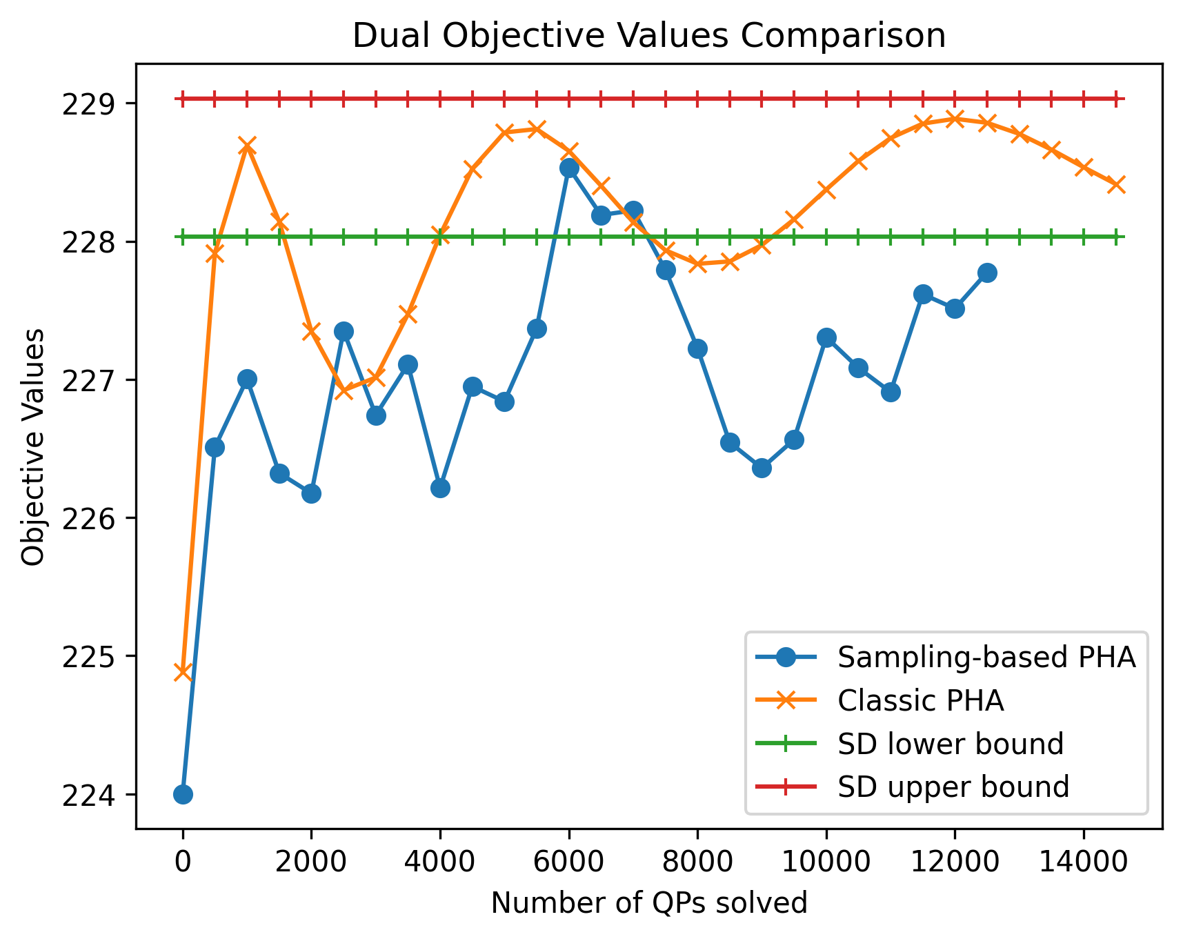
(a) lands3

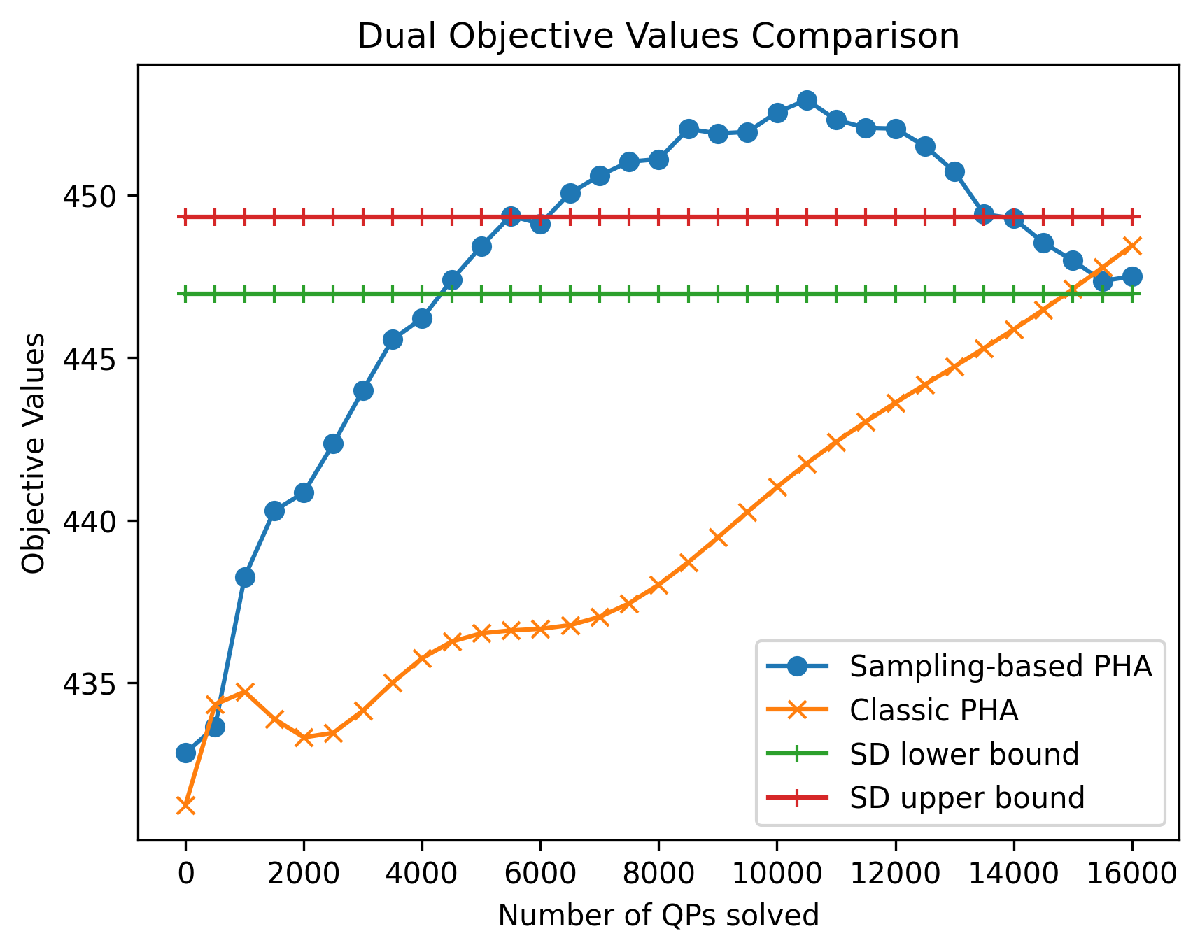
(b) pgp2

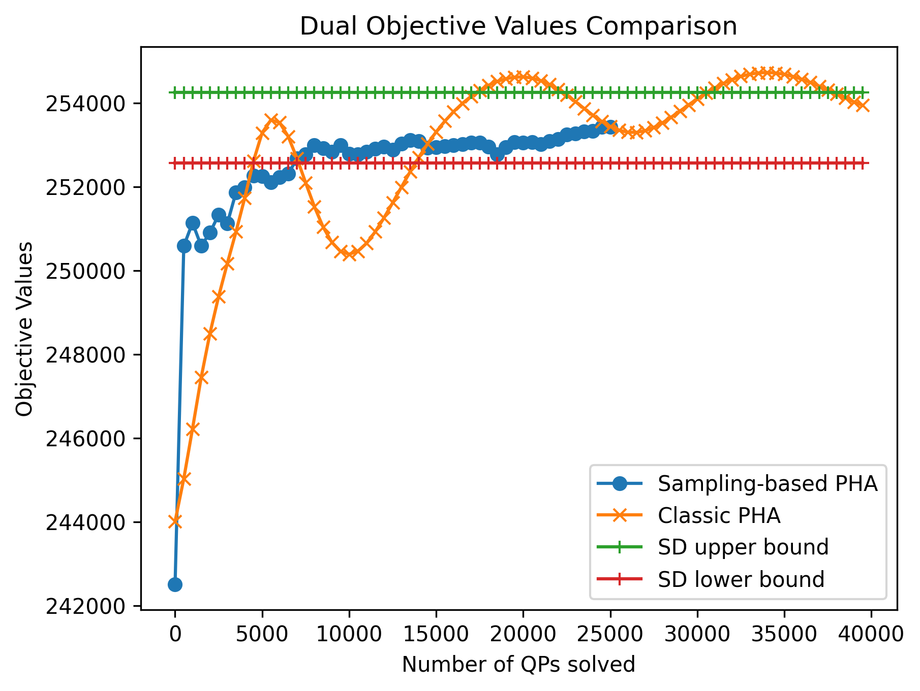
(c) 20-term

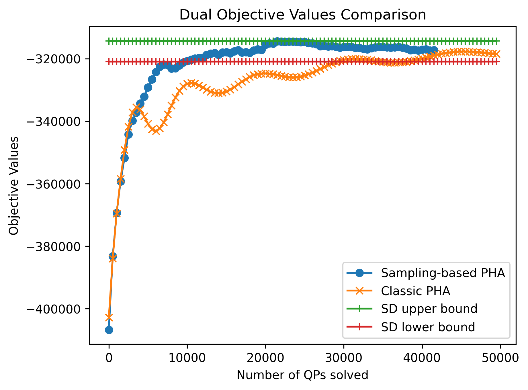
(d) baa99-20

Remark: (1)The objective function values of sampling-based PHA reflect the submartingale property we have shown in Corollary 3.9.1. On the other hand, the classic PHA does not have such property. (2) For the problems which need more scenarios to convergence, the sampling-based PH algorithm tends to convergence faster than classic PH algorithm. In other word, the sampling-based PH algorithm is more data efficient and more scalable than the classic PH algorithm.

5 Conclusion

We propose a novel sampling-based PH algorithm for large-scale stochastic optimization problems. Compared with classic PH algorithm, the proposed approach (a) does not need to know the explicit form of distribution of the random variables; (b) allows dynamic update of the sample size; (c) uses the conjugate subgradient direction and line-search to update the dual variables (d) implicitly updates the penalty parameter based on the principles of optimization. The illustrative experimental results show that it has good practical performance.

References

• [1] N. Aydin. Sampling based progressive hedging algorithms for stochastic programming problems. 2012.
• [2] A. S. Bandeira, K. Scheinberg, and L. N. Vicente. Convergence of trust-region methods based on probabilistic models. SIAM Journal on Optimization, 24(3):1238–1264, 2014.
• [3] G. Bareilles, Y. Laguel, D. Grishchenko, F. Iutzeler, and J. Malick. Randomized progressive hedging methods for multi-stage stochastic programming. Annals of Operations Research, 295(2):535–560, 2020.
• [4] J. R. Birge and F. Louveaux. Introduction to stochastic programming. Springer Science & Business Media, 2011.
• [5] L. Bottou and O. Bousquet. The tradeoffs of large scale learning. Advances in neural information processing systems, 20, 2007.
• [6] S. Boyd, N. Parikh, E. Chu, B. Peleato, J. Eckstein, et al. Distributed optimization and statistical learning via the alternating direction method of multipliers. Foundations and Trends® in Machine learning, 3(1):1–122, 2011.
• [7] S. P. Boyd and L. Vandenberghe. Convex optimization. Cambridge university press, 2004.
• [8] F. E. Curtis and K. Scheinberg. Optimization methods for supervised machine learning: From linear models to deep learning. In Leading Developments from INFORMS Communities, pages 89–114. INFORMS, 2017.
• [9] S. Diao and S. Sen. A reliability theory of compromise decisions for large-scale stochastic programs. arXiv preprint arXiv:2405.10414, 2024.
• [10] G. Grimmett and D. Stirzaker. Probability and random processes. Oxford university press, 2020.
• [11] J. L. Higle and S. Sen. Stochastic decomposition: An algorithm for two-stage linear programs with recourse. Mathematics of operations research, 16(3):650–669, 1991.
• [12] J. L. Higle and S. Sen. Finite master programs in regularized stochastic decomposition. Mathematical Programming, 67(1):143–168, 1994.
• [13] X.-B. Jin, X.-Y. Zhang, K. Huang, and G.-G. Geng. Stochastic conjugate gradient algorithm with variance reduction. IEEE Transactions on Neural Networks and Learning Systems, 30(5):1360–1369, 2018.
• [14] W.-K. Mak, D. P. Morton, and R. K. Wood. Monte carlo bounding techniques for determining solution quality in stochastic programs. Operations research letters, 24(1-2):47–56, 1999.
• [15] J. Martens et al. Deep learning via hessian-free optimization. In ICML, volume 27, pages 735–742, 2010.
• [16] A. Nedić and D. Bertsekas. Convergence rate of incremental subgradient algorithms. Stochastic optimization: algorithms and applications, pages 223–264, 2001.
• [17] J. Nocedal and S. Wright. Numerical Optimization. Springer Science & Business Media, 2006.
• [18] C. Paquette and K. Scheinberg. A stochastic line search method with expected complexity analysis. SIAM Journal on Optimization, 30(1):349–376, 2020.
• [19] H. Robbins and S. Monro. A stochastic approximation method. The annals of mathematical statistics, pages 400–407, 1951.
• [20] R. T. Rockafellar and R. J.-B. Wets. Scenarios and policy aggregation in optimization under uncertainty. Mathematics of operations research, 16(1):119–147, 1991.
• [21] A. Ruszczyński and A. Shapiro. Stochastic programming models. Handbooks in operations research and management science, 10:1–64, 2003.
• [22] S. Sen and Y. Liu. Mitigating uncertainty via compromise decisions in two-stage stochastic linear programming: Variance reduction. Operations Research, 64(6):1422–1437, 2016.
• [23] A. Shapiro and T. Homem-de Mello. A simulation-based approach to two-stage stochastic programming with recourse. Mathematical Programming, 81(3):301–325, 1998.
• [24] V. N. Vapnik, V. Vapnik, et al. Statistical learning theory. 1998.
• [25] J.-P. Watson and D. L. Woodruff. Progressive hedging innovations for a class of stochastic mixed-integer resource allocation problems. Computational Management Science, 8:355–370, 2011.
• [26] P. Wolfe. Note on a method of conjugate subgradients for minimizing nondifferentiable functions. Mathematical Programming, 7:380–383, 1974.
• [27] P. Wolfe. A method of conjugate subgradients for minimizing nondifferentiable functions. In Nondifferentiable optimization, pages 145–173. Springer, 1975.
• [28] Z. Yang. Adaptive stochastic conjugate gradient for machine learning. Expert Systems with Applications, page 117719, 2022.
• [29] F. X. X. Yu, A. T. Suresh, K. M. Choromanski, D. N. Holtmann-Rice, and S. Kumar. Orthogonal random features. Advances in neural information processing systems, 29:1975–1983, 2016.
• [30] S. Zehtabian and F. Bastin. Penalty parameter update strategies in progressive hedging algorithm. Cirrelt Montreal, QC, Canada, 2016.