11email: {rzh,eustice,maanigj}@umich.edu 22institutetext: Amazon Lab126, Sunnyvale CA 94089, USA
22email: {zhemiz,minnsun,ghasemal,chkuo,senarnie}@amazon.com
Correspondence-Free SE(3) Point Cloud Registration in RKHS via Unsupervised Equivariant Learning
Abstract
This paper introduces a robust unsupervised SE(3) point cloud registration method that operates without requiring point correspondences. The method frames point clouds as functions in a reproducing kernel Hilbert space (RKHS), leveraging SE(3)-equivariant features for direct feature space registration. A novel RKHS distance metric is proposed, offering reliable performance amidst noise, outliers, and asymmetrical data. An unsupervised training approach is introduced to effectively handle limited ground truth data, facilitating adaptation to real datasets. The proposed method outperforms classical and supervised methods in terms of registration accuracy on both synthetic (ModelNet40) and real-world (ETH3D) noisy, outlier-rich datasets. To our best knowledge, this marks the first instance of successful real RGB-D odometry data registration using an equivariant method. The code is available at https://sites.google.com/view/eccv24-equivalign.
Keywords:
Point Cloud Registration Equivariant Learning Kernel Method Unsupervised Learning1 Introduction
Point cloud registration estimates the relative transformation between two sets of 3D spatial observations [3, 9, 34, 61, 64]. It is commonly formulated as a nonlinear optimization problem, with data inputs from varied sensors such as RGB-D cameras, stereo cameras, and LiDAR. This technique is vital in computer vision and robotics, especially for applications like visual odometry [29] and 3D reconstruction [56]. Despite its wide use, point cloud registration encounters numerous challenges. These include complexities in nonlinear optimization on Riemannian manifolds, addressing non-overlapping observations, and mitigating the impact of sensor noise and outliers [58, 42]. These challenges stem from two tightly coupled components in traditional point cloud registration: point representations and correspondences. Point representation refers to the actual format of the point data in the process. Given a representation, point correspondences are related to the construction of the residuals from point pairings.
Classical methods represent points using hand-crafted geometric primitives such as 3D point coordinates [3, 47], planes [9], Gaussian mixtures [34, 28], and surfels [56, 8]. These representations, typically as low-dimensional vectors, allow residuals to be computed directly as Euclidean or Mahalanobis distances. However, they often struggle with handling noisy and outlier-rich observations because they rely on strict data correspondence. Correct data association is challenging [30], especially when the features are not discriminative enough. Robust optimization strategies are often needed to minimize these limitations [58].
In contrast, Continuous Visual Odometry (CVO) [24, 13, 61] introduces a robust registration framework that represents each point cloud as a continuous function in RKHS. Its iterative registration process minimizes the distance of the two point cloud functions in RKHS and doesn’t require strict pair-wise point correspondences. Although it demonstrates superior robustness compared to classical geometric registration methods, the iterative framework is constrained by limited expressiveness because the framework is not differentiable.
Advancements in deep neural networks bring differentiable point set registration by learning point representations that embody geometric invariance [41, 60, 31, 19, 54, 10] or equivariance. Invariant-feature-based approaches focus on learning point-wise local and global features that remain invariant under pose transformations, leading to semantic-aware data association [59, 27]. Once one-to-one correspondences are established, methods like RANSAC or weighted SVD are employed for pose regression [22, 3]. However, challenges persist in the generalization of invariant learning. During training, excessive data augmentation is required for sampling transformations in and simulating the noise perturbations. Besides, their supervised nature rely on extensive ground truth labels.
Equivariant-feature-based methods provide an alternative deep representation for point clouds [15, 17, 55, 50]. Equivariance is a property for a map such that given a transformation in the input, the output changes in a predictable way determined by the input transformation: A function is equivariant to a set of transformations , if for any , Recent strides in equivariant learning have expanded to include [18, 65], [7, 64], and [45] equivariant networks. Compared to invariant feature-based methods, these networks relax the need for extensive data augmentation and thereby leading to improved generalization[64]. While equivariant learning has shown promise within physics and chemistry, its effectiveness in real-world robotic tasks like point cloud registration is not well-established. For existing works, common practices include training a shape embedding to re-establish the one-to-one correspondence [65], or pooling point-wise equivariant features into global equivariance features [7, 64]. These approaches undermine the complexities of the noisy and outlier-rich real data where the two input point clouds are not exactly the same, i.e., the equivariance does not fully hold.
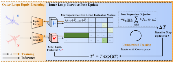
In this work, we introduce an unsupervised feature space registration framework, EquivAlign, as depicted in Figure 2. This framework focuses on learning point-wise representations that respect the intricate geometric structure in feature space. The proposed equivariant kernel learning interprets the neural feature embeddings of these point clouds as nonparametric functions within a specified RKHS. This unique perspective allows for feature space registration without strict correspondences, further supporting the fully differentiable and unsupervised nature of our proposed method. The contributions are outlined as follows:
-
1.
An iterative and fully differentiable registration framework that facilitates correspondence-free feature space pose regression, enabling robustness to unseen noise and outliers.
-
2.
A lightweight feature representation equivariant to 3D rotations and translations via a novel direct sum construction. This construction is modular and can easily benefit from future advances in equivariant encoders.
-
3.
An unsupervised inner-outer loop training scheme for equivariant feature learning, incorporating a curriculum learning schedule, demonstrates enhanced accuracy compared to classical and supervised baselines and shows effectiveness in real-world applications.
2 Related Work
2.1 Classical Registration with ICP and GMM
The Iterative Closest Points (ICP) algorithm and its variants use hand-crafted geometric primitives like coordinates and surfaces as the point representation [3, 9, 35, 47]. They alternatively search correspondences with the closest geometric distances and then obtain pose estimates with the one-to-one data association. Later works incorporate invariant features into the association for improved robustness, including color [48, 36], intensity [38], and semantic features [37].
Gaussian Mixture Model (GMM) registration represents point clouds as probabilistic densities [28, 6, 12, 20, 21, 26]. Gaussian mixture models are fitted to the point cloud inputs, followed by soft data associations. Normal Distribution Transform (NDT) provides a particularly efficient way of modeling local geometric structures through voxelization [4, 34].
2.2 Registration with Invariant Feature Matching
Early works like FPFH [44] create histogram-based local invariant features that are used in global registration. Deep invariant features provide a richer point representation that assists in feature space correspondence search. Encoders such as MLP [41], Graphic Neural Networks [54], and KPConv [49] are used for feature extraction that contribute to permutations invariance and local structures. In the correspondence step, direct supervision on inlier and outlier matches is usually required. This class of methods requires one-to-one pairwise matching, with either RANSAC or weighted SVD. To make the data association robust, complicated outlier rejection training mechanisms are adopted, assuming enough labeled training data. FCGF [11] uses feature space metric learning with negative mining to filter the outliers. It samples both positive inliers and negative outliers so as to prevent the features being biased on the positive samples. Coarse-to-fine strategies in D3FeatNet [1], DCP [53], Cofinet [59], PREDATOR [27], and GeoTransformer [42] enhance match precision by initially focusing on overlapping areas with superpixel or local patch matching, followed by finer point correspondences. Particularly, PREDATOR [27] and GeoTransformer [42] leverage Graph Neural Networks (GNN) and cross-attention mechanisms for feature enhancement and adopt top-K neighbors for associations. These deep learning techniques, integrated with robust optimization methods like those in Teaser++ [58], represent a significant stride in achieving more accurate and reliable point cloud registration. However, their methods rely on costly labeling of ground truth and extensive data augmentation for generalization.
2.3 Equivariant Learning and Applications in Registration
In the field of equivariant learning and registration, group convolution extends to various domains, beginning with Cohen’s [15] work on lifting convolution kernels to rotations for image processing. This includes both discretizing rotations into finite groups like the dihedral group and continuous sampling with Monte Carlo [33]. For 3D data, the icosahedron convolution theory [14] and applications such as EPN [7] and E2PN [64] leverage finite group discretization in point cloud analysis. These methods efficiently encode features across various angles in . Additionally, to learn translation-equivariant features, they incorporate traditional convolution layers.
Another approach involves continuous steerable feature maps in higher-order group representations, demanding significant computational resources for calculating coefficients [50, 16, 23]. VectorNeuron [18] offers a more computationally efficient solution using only type-1 features. Existing equivariant methods with continuous group representations are mainly applied in physics and chemistry, whereas their performance in real robotics data requires further testing. Inspired by TFN [50] and VectorNeuron [18], we construct a lightweight equivariant representation as a direct sum of point coordinates and steerable vectors to enable efficient translation and rotation equivariance.
2.4 Nonparametric Registration in RKHS
Continuous Visual Odometry (CVO) [25] introduces a novel point cloud registration formulation by representing colored point clouds as continuous functions in an RKHS and aligns these functions using gradient ascent. The optimization step size is estimated through a fourth-order Taylor expansion. Kernel correlation [51], a specific instance of CVO, focuses solely on geometric registration and optimizes the loss using a first-order approximation. AdaptiveCVO [32] optimizes the kernel length scale, while SemanticCVO [61] integrates hierarchical semantic information, such as color and semantics, with geometric data.
EquivAlign sets itself apart from the above methods by reformulating the approach to ensure differentiability, thus enabling the learning of features meticulously designed for the registration task. Such features are required to support iterative pose updates at the inference stage, underscoring the necessity for equivariant features. In contrast, while SemanticCVO can also leverage deep features, it employs them in a non-differentiable fashion, depending on features derived from a pretrained network.
3 Problem Formulation
Before delving into the proposed EquivAlign in the following section, we briefly review the notations and core principles of the problem.
Consider two (finite) collections of points, , , with not necessarily being equal. We aim to find an element , which minimizes a distance metric between two point clouds and :
| (1) |
An group element with acting on a point is given by .
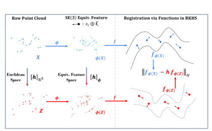
The point clouds, and , are first represented as functions that live in some reproducing kernel Hilbert space (RKHS), denoted as . The group action induces an action on the RKHS, , denoted as . Inspired by this observation, we set . Furthermore, each point might contain pose-invariant information in different dimensions, such as color or intensity, described by a point in an inner product space, . To represent pose-invariant information, we introduce two labeling functions, and for the two point clouds with , respectively. With the kernel formulation [5], the point cloud functions are
| (2) |
where the kernels are symmetric and positive definite functions. .
To measure the alignment of the two point clouds given an isometry transformation that preserves norms, we can use the distance between the two point cloud functions [13]
| (3) |
The distance is well-defined because RKHS is endowed with a valid inner product. With the reproducing property [2], each inner product becomes
4 EquivAlign Framework
Figure 2 illustrates the EquivAlign framework. The process begins with the introduction of a lightweight equivariant feature representation as detailed in Section 4.1. Subsequently, we focus on optimizing the pose and kernel parameters within this feature space (Sections 4.2 and 4.3). The training phase is distinctive due to the disparate stages and frequencies at which updates for the equivariant feature encoder, as well as for the kernel and pose, take place. To address this, we perform an unsupervised inner-outer loop learning strategy with curriculum learning, as discussed in Section 4.5.
4.1 Equivariant Point Representation
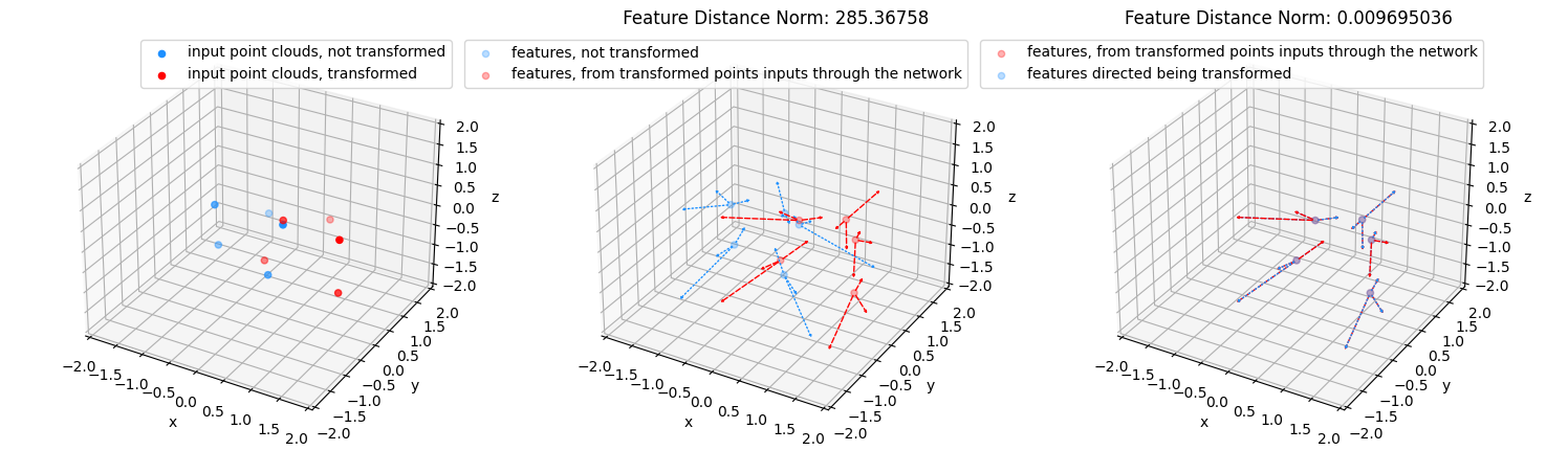
Unlike raw 3D coordinates, feature maps extracted from deep neural networks produce a more expressive representation of the point clouds. Instead of representing each point as an element in as in CVO, we design equivariant features to represent them, : a direct sum of ’s coordinate and multiple channels of -dimensional steerable vectors , with being the equivariant encoder with weights . The steerable features are a specific type-1 feature [50] for rotations in VectorNeuron [18]. VectorNeuron proposes that -equivariance can be realized by centering the point cloud coordinates. However, in real applications, the two input point clouds do not fully overlap. Thus, we cannot simply centralize them and process the rotation-only registration. Instead, we incorporate an additional type-0 feature—the 3D coordinate itself. Each channel of this representation can be visualized as a vector field defined on , as shown in Figure 3. This straightforward yet effective representation is modular, allowing for easy adaptation to future advancements in equivariant encoders.
The rotation and translation of the pose can be applied directly to the point-wise feature representations as follows:
| (4) |
The rotation’s action on the features is on both the coordinates and the steerable vectors. The translation’s action will only alter the coordinates but will not affect the vector field elements’ directions.
The linear multiplications by weights and the nonlinearity [18] that acts solely on the steerable features can be defined as follows:
| (5) |
The graph convolution over point is similar to DGCNN [54] and VectorNeuron [18], but with the additional direct sum of 3D coordinate itself:
| (6) |
where are the neighbors’ features and are the weights to learn.
4.2 Pose Optimization and Kernel Learning in the Feature Space
To estimate the transformation, the objective is to minimize the distance between the two functions within the RKHS:
| (7) |
where each function is represented as . Let and , then we have:
As the label function (color, intensity, etc.) remains invariant under the pose change, the following variables can be treated as constants: . The final objective function becomes:
| (8) |
4.3 Kernel Choice
The RKHS, in which the point cloud functions reside, necessitates a well-defined Mercer kernel [2]. Characterized by a hyperparameter , this kernel is a function of two variables within the equivariant feature space and has to be symmetric and positive-definite: .
The selection of kernel is guided by two critical criteria. Firstly, it necessitates a minimal number of hyperparameters. In the classical CVO framework [61], the kernel operates on three-dimensional inputs, where hyperparameters significantly influence the outcomes. Managing these hyperparameters becomes increasingly complex with higher-dimensional inputs, such as the direct sum of the 3D coordinate and the multi-channel steerable vectors. Secondly, the kernel’s hyperparameters should be interpretable, enabling an understanding of its impact on the model’s performance. The kernel is defined as the product of the Radial Basis Function (RBF) kernel and the hyperbolic tangent kernel, as described in [43]:
| (9) |
The RBF kernel is utilized for the coordinate part and the hyperbolic tangent kernel for the steerable feature maps. The RBF kernel includes a kernel parameter, the lengthscale , which is optimized during pose inference:
| (10) |
The RBF kernel is adopted to leverage the lengthscale parameter in promoting sparsity and minimizing the number of non-trivial terms in the loss calculation. A parameterized kernel is not selected for the steerable vectors to decrease the number of parameters requiring optimization during test time.
4.4 Inference
During the inference stage, the goal is to minimize the distance between two functions with respect to the pose and the kernel parameter , while keeping the encoder weights fixed:
| (11) |
It’s important to note that for each iteration of pose optimization, there’s no need to process the transformed point cloud through the encoder again. Instead, the approach involves directly transforming the equivariant features and re-evaluating the kernels during the loss calculation.
4.5 Unsupervised Training of Equivariant Encoder
In practical scenarios such as visual odometry, ground truth transformation labels are often scarce. To adapt the encoder weights to new environments, unsupervised bi-level training [40] is employed:
| (12) |
During training, the two point clouds are initially processed through the equivariant encoder to derive the point-wise equivariant features . Subsequently, in each iteration, the loss is minimized with respect to the transformation and the kernel parameter , facilitating a stepwise update of the transformation. Using the latest pose estimate , the gradient is retained in the computation graph, and the encoder parameters are updated. This training strategy does not require ground truth pose labels.
Additional aspects of the training procedure are necessary to ensure satisfactory convergence properties. A curriculum training strategy is employed to initiate training from random initial weights, starting with smaller angles at and progressively advancing to larger angles up to . Moreover, there is a tendency for the kernel parameter to change too rapidly, potentially causing its values effectively becoming zero. To mitigate this issue, a learning rate that is 100 times smaller is utilized specifically for updating the kernel lengthscale .
5 Experiments
In this section, qualitative and quantitative experimental results are presented on both a simulated dataset, the ModelNet40 dataset [57], and a real-world RGB-D dataset, ETH3D [46]. The assessment focuses on EquivAlign’s registration accuracy in rotations and translations, along with its robustness to different perturbations. The implementation is based on Pytorch [39] and PyPose [52].
Baselines: Three types of baselines are chosen: a) Classical non-learning registration methods, including ICP [3], GICP [47] and the classical CVO [61]. For a fair comparison, CVO’s label function is set to to exclude extra information like color. b) Invariant feature-matching based methods, including RANSAC [22] with FPFH features, FGR [62] with FPFH features, and GeoTransformer [42]. GeoTransformer’s official implementation is used, with the author-provided pretrained weights on ModelNet40 and our custom-trained weights on ETH3D. c) An equivariant feature method based on finite groups, E2PN [64], trained under the same setup as EquivAlign.
5.1 Simulation Dataset: ModelNet40 Registration
Setup: In this experiment, we perform point cloud registration of all methods on the ModelNet40 dataset, which comprises shapes generated from 3D CAD models. To avoid the pose ambiguity of objects with symmetric rotational shapes, only the non-rotational symmetric categories are used in this experiment, with 60% training data, 20% validation data, and 20% test data. A point cloud is generated by randomly subsampling 1,024 points on the surface, and it is randomly rotated to form a pair. The initial rotation angle is set at and around random axes. The error metric is the mean of the matrix logarithm error between the resulting pose and the ground truth pose, i.e., . To assess the model’s robustness under various noise perturbations, three types of noises are injected: a) Gaussian noise distributed along each point’s surface normal. b) uniformly distributed outliers along each point’s surface normal c) up to random cropping along a random axis. These noises are not applied during training time for EquivAlign and E2PN. Note that only GeoTransformer includes these perturbations as data augmentations in its pretrained model.
| Type | Method | Test Init Angle | Test Init Angle | ||||
|---|---|---|---|---|---|---|---|
| Non-Learning | ICP | 1.11 | 1.21 | 1.38 | 34.52 | 36.15 | 38.00 |
| GICP | 2.44 | 2.74 | 2.53 | 49.88 | 46.42 | 48.40 | |
| Geometric-CVO | 5.67 | 5.93 | 6.28 | 23.90 | 26.92 | 30.84 | |
| Invariant Features | FPFH + RANSAC | 0.02 | 42.50 | 42.43 | 0.73 | 85.63 | 85.60 |
| FPFH + FGR | 0.07 | 2.27 | 12.62 | 0.14 | 11.69 | 43.88 | |
| GeoTransformer | 0.67 | 0.71 | 0.92 | 42.82 | 43.28 | 42.58 | |
| Equivariant Features | E2PN | 3.86 | 46.84 | 70.88 | 3.78 | 48.19 | 70.61 |
| EquivAlign | 0.61 | 1.93 | 1.96 | 1.14 | 4.08 | 4.12 | |
| Type | Method | Test Init Angle | Test Init Angle | ||||
| crop | crop | crop | crop | crop | crop | ||
| Non-Learning | ICP | 2.25 | 2.73 | 5.94 | 37.00 | 39.23 | 45.04 |
| GICP | 3.33 | 3.34 | 5.68 | 49.28 | 49.90 | 53.78 | |
| Geometric-CVO | 11.04 | 15.90 | 23.40 | 31.77 | 45.24 | 52.47 | |
| Invariant Features | FPFH + RANSAC | 42.56 | 42.37 | 43.10 | 85.60 | 85.51 | 85.17 |
| FPFH + FGR | 37.93 | 44.73 | 57.15 | 78.66 | 82.22 | 90.94 | |
| GeoTransformer | 1.13 | 1.22 | 1.39 | 41.41 | 42.04 | 45.45 | |
| Equivariant Features | E2PN | 76.90 | 84.30 | 92.41 | 76.06 | 83.42 | 94.70 |
| EquivAlign | 9.88 | 14.23 | 19.20 | 15.01 | 28.87 | 43.32 | |
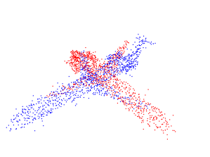
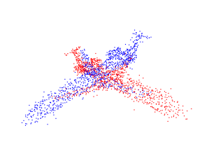
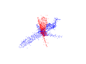
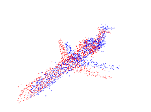
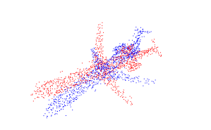
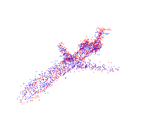
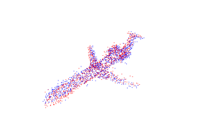
Results: The quantitative results are presented in Table 1 and the qualitative results are shown in Figure 4. We denote the variance of the Gaussian noise as and the ratio for the uniform outlier perturbation as .
In noise-free conditions, both classical and proposed methods excel at smaller angles (), with invariant feature-matching methods showing lower errors compared to equivariant-learning-based approaches. EquivAlign demonstrates performance on par with classical ICP methods and superior to E2PN. However, at initial angles of , ICP and GICP show larger errors due to their reliance on accurate initial guesses for data association. In these scenarios, EquivAlign surpasses E2PN, but invariant feature-matching methods achieve the best results.
When encountering Gaussian noise, EquivAlign reaches a slightly better accuracy than the invariant feature matching methods at (except GeoTransformer) and is the best-performing method at . GeoTransformer tops the benchmark at . Similar to the noise-less situation, non-learning methods’ result degenerate at larger initial angles.
With uniformly distributed outliers, methods assuming Gaussian errors will degrade. Invariant feature matching is severely affected by this type of perturbation and fails to register at smaller or larger angles, unless extensive data augmentation is used during training. ICP-based methods can reach satisfactory results at small angles but not larger ones. EquivAlign remains largely unaffected by this perturbation, achieving the best results at by a significant margin and performing comparably to ICP-type methods at . This demonstrates how the expressiveness of equivariant features helps in the robustness of the registration process, even when only noise-free data is used in training.
In tests involving random cropping of input data (with no cropping in training), as reported in Table 1 (Bottom), all methods experience performance dips. Similar to the third case, ICP-based methods are not substantially affected by the cropping at but are easily trapped in the local minima at larger angles. Classical invariant feature-based baselines cannot converge at either initial angle, but with sufficient data augmentation, GeoTransformer becomes the best-performing method. Both equivariant methods also experienced larger errors, not as severe as the classical invariant feature matching methods though. The proposed learning-based RKHS formulation natively annihilates the outlier disturbance because, at larger distances, the kernel will return trivial values. In contrast, as E2PN directly performs global pooling over all the points to obtain a single global feature, missing cropped components will reduce the quality of the global feature, especially when the crop is unseen in the training data.
5.2 Real Dataset: ETH3D RGB-D Registration
| Type | Method | Rot. Error | Trans. Error | ||
|---|---|---|---|---|---|
| Mean | STD. | Mean | STD. | ||
| Non-Learning | ICP | 0.88 | 1.30 | 0.03 | 0.05 |
| GICP | 0.69 | 3.54 | 0.02 | 0.11 | |
| Geometric-CVO | 0.71 | 0.94 | 0.02 | 0.02 | |
| Invariant Features | FPFH + RANSAC | 8.75 | 2.95 | 0.17 | 0.40 |
| FPFH + FGR | 3.60 | 12.61 | 0.08 | 0.17 | |
| GeoTransformer | 2.23 | 13.09 | 0.07 | 0.31 | |
| Equivariant Features | E2PN | 5.20 | NA | NA | NA |
| EquivAlign | 0.53 | 0.99 | 0.01 | 0.02 | |
![[Uncaptioned image]](/html/2407.20223/assets/x11.png)
Setup: In this experiment, EquivAlign is benchmarked against other baselines using a real RGB-D dataset. We utilize the ETH3D dataset [46], comprising real indoor and outdoor RGB-D images. In this setup, two point cloud pairs are sampled sequentially. Unlike the simulated ModelNet40 dataset, a pair of point clouds will not fully overlap even without noise injections due to the viewpoint change. Additionally, the ground truth pose will contain rotation and translation but at smaller angles than the ModelNet40 experiment. A random rotation perturbation of is injected into each pair of testing data. 6 sequences are used for training: (\seqsplitcable_3, \seqsplitceiling_1, \seqsplitrepetitive, \seqspliteinstein_2, \seqsplitsfm_house_loop, \seqsplitdesk_3), 2 sequences for validation: (\seqsplitmannequin_3, \seqsplitsfm_garden), and 4 sequences for testing: (\seqsplitsfm_lab_room_1, \seqsplitplant_1, \seqsplitsfm_bench, \seqsplittable_3). Given the varying number of frames in each sequence, frame pairs are subsampled to ensure no more than 1000 pairs per sequence. This results in 5919 training instances, 2000 validation instances, and 2702 test instances. For all the methods, input point clouds are downsampled into 1024 points with the \seqsplitfarthest_point_down_sample method from Open3D [63]. For a fair comparison, color information is excluded in EquivAlign by setting the label function in Eq. (2) as the baselines similarly abstain from using color.
Results: The quantitative results are shown in Table 2. On the test sequences, EquivAlign demonstrates the best accuracy in both rotation and translation evaluations, with a rotation error, translation error, and lowest variations. The invariant feature-based baselines have significantly larger test errors. This is due to the challenge of generalizing to real-world noise, particularly for supervised learning methods. ICP-based methods have comparable translation errors, but their rotation error is and larger, respectively. This comparison indicates that EquivAlign produces fine-grained registration alone in real data and thus can be adopted in applications like frame-to-frame pose tracking. It does not have the necessity of using coarse-to-fine strategies with ICP, as adopted in recent invariant-learning-based works like PREDATOR [27].
Moreover, the other equivariant baseline, E2PN, is also not as accurate as EquivAlign, though it is correspondence-free and has superior global registration ability. We argue that there are three potential reasons behind this: First, E2PN uses a finite group rotation representation on equivariance learning, resulting in a much faster running speed via feature permutation. However, the discretization comes at a cost; that is, it will have resolution challenges at fine-grained registration, especially compared to EquivAlign’s continuous rotation representation. Secondly, EquivAlign does not require training labels and thus is not tightly coupled to the training data distribution. In contrast, E2PN needs ground truth supervision, which means there would be overfitting challenges if the test set is a new scene. Thirdly, EquivAlign adopts the RKHS representation whose kernel can eliminate the influence of non-overlapped areas, while E2PN assumes complete symmetry of the input pair, which is often violated in real data. Recent works such as SE3-Transformer [23] and GeoTransformer [42] attempt to bring the attention mechanism to address this issue. But training the attention network will also need ground truth labels.
5.3 Ablation Study
5.3.1 Kernel Choice
The chosen kernel, although not our primary focus, prefers minimal hyperparameters and is interpretable, or any suitable kernel satisfying these. Even with a 3D kernel in the classical CVO [61], the hyperparameters significantly impact the results. More complexity in controlling them could arise with higher dimensional inputs like the higher dimensional steerable vectors. The current kernel choice links RBF kernel lengthscales to Euclidean point distances, whereas the kernel only considers steerable vector directions. To demonstrate that, we train and test the network with a single RBF kernel on ModelNet40 of 45∘ initial angles in Table 3 (a).
5.3.2 Initial Kernel Parameter
EquivAlign has a hyperparameter, the kernel lengthscale , which controls the coarse-grain and fine-grain resolution of the loss [13, 61]. It is optimized during pose regression but still requires an initial value. In this ablation study shown in Table 3 (b), we test how the initial lengthscale will affect the registration accuracy on the ModelNet40 dataset. The outcome corroborates insights from the CVO works: Registering at larger angles necessitates a greater initial lengthscale for a comprehensive global perspective.
5.3.3 Curriculum Learning vs. Direct Training
As an unsupervised approach, one significant challenge we addressed was the bootstrap of the randomly-initialized network weights. To investigate this issue, we conducted an ablation study between curriculum-based training and direct training at maximal angular perturbations, as presented in Table 3 (c). Our findings show that a gradual curriculum with incremental steps significantly enhances model accuracy and reduces uncertainty, highlighting the effectiveness of curriculum learning for optimizing network performance from randomly initialized weights.
| Kernel Choice | Rot. Error (∘) |
|---|---|
| Init Angle | |
| RBFTanh kernel | 0.29 |
| RBF kernel only | 81.97 |
![[Uncaptioned image]](/html/2407.20223/assets/figs/ablation_rotation_ell.png)
| Curriculum | ||||
|---|---|---|---|---|
| Mean | STD. | Mean | STD. | |
| Init Angle: | 2.73 | 9.1 | 0.29 | 0.469 |
6 Limitations and Conclusion
There are trade-offs with our method, including lengthy training times and reduced performance with limited overlap. Our unsupervised training approach uses a curriculum learning strategy that progresses from smaller to larger rotations, resulting in extended training times. Training on the ModelNet40 dataset with 8 NVIDIA V100 GPUs takes a week for registrations. Performance decreases in low-overlap scenarios, as indicated in Table 1, where 60% overlap (20% cropping) reduces registration accuracy. However, data augmentation, longer training cycles, and a denser curriculum can improve low-overlap performance, while a sparser curriculum can reduce training time. Besides the extended training time, our method has an inference time of 0.03 to 0.1 seconds per iteration on a single V100 GPU. Future directions include incorporating -equivariant transformers into the encoder to capture more extended feature correlations, enhancing robustness and efficiency.
In summary, this paper introduces a differentiable, iterative point cloud registration framework that leverages correspondence-free pose regression in RKHS. EquivAlign achieves fine-grained feature space registration and effectively handles noise, outliers, and limited labeled data. Results on ModelNet40 and ETH3D datasets show our method outperforming established methods particularly in noise resilience. This study lays a foundation for further research in unsupervised equivariant learning within 3D vision and opens its application to numerous fields, including but not limited to robotics and the medical domain.
References
- [1] Bai, X., Luo, Z., Zhou, L., Fu, H., Quan, L., Tai, C.L.: D3feat: Joint learning of dense detection and description of 3D local features. In: Proc. IEEE Conf. Comput. Vis. Pattern Recog. pp. 6359–6367 (2020)
- [2] Berlinet, A., Thomas-Agnan, C.: Reproducing Kernel Hilbert Space in Probability and Statistics. Springer Science and Business Media (01 2004). https://doi.org/10.1007/978-1-4419-9096-9
- [3] Besl, P.J., McKay, N.D.: A method for registration of 3-d shapes. IEEE Trans. Pattern Anal. Mach. Intell. 14(2), 239–256 (Feb 1992). https://doi.org/10.1109/34.121791
- [4] Biber, P., Fleck, S., Straßer, W.: A probabilistic framework for robust and accurate matching of point clouds. In: Joint Pattern Recognition Symposium. pp. 480–487. Springer (2004)
- [5] Bishop, C.M.: Pattern recognition and machine learning. Springer (2006)
- [6] Campbell, D., Petersson, L.: An adaptive data representation for robust point-set registration and merging. In: Proc. IEEE Int. Conf. Comput. Vis. pp. 4292–4300 (2015)
- [7] Chen, H., Liu, S., Chen, W., Li, H., Hill, R.: Equivariant point network for 3D point cloud analysis. In: Proc. IEEE Conf. Comput. Vis. Pattern Recog. pp. 14514–14523 (2021)
- [8] Chen, X., Milioto, A., Palazzolo, E., Giguere, P., Behley, J., Stachniss, C.: Suma++: Efficient lidar-based semantic slam. In: Proc. IEEE/RSJ Int. Conf. Intell. Robots and Syst. pp. 4530–4537. IEEE (2019)
- [9] Chen, Y., Medioni, G.G.: Object modeling by registration of multiple range images. Image Vision Comput. 10(3), 145–155 (1992)
- [10] Choy, C., Park, J., Koltun, V.: Fully convolutional geometric features. In: Proceedings of the IEEE International Conference on Computer Vision. pp. 8958–8966 (2019)
- [11] Choy, C., Park, J., Koltun, V.: Fully convolutional geometric features. In: Proc. IEEE Int. Conf. Comput. Vis. pp. 8958–8966 (2019)
- [12] Chui, H., Rangarajan, A.: A feature registration framework using mixture models. In: Proceedings IEEE Workshop on Mathematical Methods in Biomedical Image Analysis. pp. 190–197. IEEE (2000)
- [13] Clark, W., Ghaffari, M., Bloch, A.: Nonparametric continuous sensor registration. J. Mach. Learning Res. 22(271), 1–50 (2021)
- [14] Cohen, T., Weiler, M., Kicanaoglu, B., Welling, M.: Gauge equivariant convolutional networks and the icosahedral CNN. In: Proc. Int. Conf. Mach. Learning. pp. 1321–1330. PMLR (2019)
- [15] Cohen, T., Welling, M.: Group equivariant convolutional networks. In: Proc. Int. Conf. Mach. Learning. pp. 2990–2999. PMLR (2016)
- [16] Cohen, T.S., Geiger, M., Köhler, J., Welling, M.: Spherical cnns. arXiv preprint arXiv:1801.10130 (2018)
- [17] Cohen, T.S., Welling, M.: Steerable cnns. arXiv preprint arXiv:1612.08498 (2016)
- [18] Deng, C., Litany, O., Duan, Y., Poulenard, A., Tagliasacchi, A., Guibas, L.J.: Vector neurons: A general framework for SO(3)-equivariant networks. In: Proc. IEEE Int. Conf. Comput. Vis. pp. 12200–12209 (2021)
- [19] Deng, H., Birdal, T., Ilic, S.: Ppfnet: Global context aware local features for robust 3d point matching. In: Proceedings of the IEEE conference on computer vision and pattern recognition. pp. 195–205 (2018)
- [20] Eckart, B., Kim, K., Kautz, J.: Hgmr: Hierarchical Gaussian mixtures for adaptive 3D registration. In: Proc. European Conf. Comput. Vis. pp. 705–721 (2018)
- [21] Evangelidis, G.D., Horaud, R.: Joint alignment of multiple point sets with batch and incremental expectation-maximization. IEEE Trans. Pattern Anal. Mach. Intell. 40(6), 1397–1410 (2017)
- [22] Fischler, M.A., Bolles, R.C.: Random sample consensus: a paradigm for model fitting with applications to image analysis and automated cartography. Communications of the ACM 24(6), 381–395 (1981)
- [23] Fuchs, F., Worrall, D., Fischer, V., Welling, M.: SE(3)-transformers: 3D roto-translation equivariant attention networks. Proc. Advances Neural Inform. Process. Syst. Conf. 33, 1970–1981 (2020)
- [24] Ghaffari, M., Clark, W., Bloch, A., Eustice, R.M., Grizzle, J.W.: Continuous direct sparse visual odometry from RGB-D images. In: Proc. Robot.: Sci. Syst. Conf. Freiburg, Germany (June 2019)
- [25] Ghaffari, M., Clark, W., Bloch, A., Eustice, R.M., Grizzle, J.W.: Continuous direct sparse visual odometry from RGB-D images. arXiv preprint arXiv:1904.02266 (2019)
- [26] Horaud, R., Forbes, F., Yguel, M., Dewaele, G., Zhang, J.: Rigid and articulated point registration with expectation conditional maximization. IEEE Trans. Pattern Anal. Mach. Intell. 33(3), 587–602 (2010)
- [27] Huang, S., Gojcic, Z., Usvyatsov, M., Wieser, A., Schindler, K.: Predator: Registration of 3D point clouds with low overlap. In: Proc. IEEE Conf. Comput. Vis. Pattern Recog. pp. 4267–4276 (2021)
- [28] Jian, B., Vemuri, B.C.: Robust point set registration using Gaussian mixture models. IEEE Trans. Pattern Anal. Mach. Intell. 33(8), 1633–1645 (Aug 2011)
- [29] Kerl, C.: Dense Visual Odometry (DVO). https://github.com/tum-vision/dvo (2013)
- [30] Li, F., Fujiwara, K., Okura, F., Matsushita, Y.: Generalized shuffled linear regression. In: Proceedings of the IEEE/CVF International Conference on Computer Vision. pp. 6474–6483 (2021)
- [31] Li, Y., Bu, R., Sun, M., Wu, W., Di, X., Chen, B.: Pointcnn: Convolution on x-transformed points. In: Proc. Advances Neural Inform. Process. Syst. Conf. pp. 820–830 (2018)
- [32] Lin, T.Y., Clark, W., Eustice, R.M., Grizzle, J.W., Bloch, A., Ghaffari, M.: Adaptive continuous visual odometry from RGB-D images. arXiv preprint arXiv:1910.00713 (2019)
- [33] MacDonald, L.E., Ramasinghe, S., Lucey, S.: Enabling equivariance for arbitrary lie groups. In: Proc. IEEE Conf. Comput. Vis. Pattern Recog. pp. 8183–8192 (2022)
- [34] Magnusson, M., Lilienthal, A., Duckett, T.: Scan registration for autonomous mining vehicles using 3D-NDT. J. Field Robot. 24(10), 803–827 (2007)
- [35] Mitra, N.J., Gelfand, N., Pottmann, H., Guibas, L.: Registration of point cloud data from a geometric optimization perspective. In: Proceedings of the 2004 Eurographics/ACM SIGGRAPH Symposium on Geometry Processing. p. 22–31. SGP ’04, Association for Computing Machinery, New York, NY, USA (2004). https://doi.org/10.1145/1057432.1057435
- [36] Park, J., Zhou, Q.Y., Koltun, V.: Colored point cloud registration revisited. In: Proc. IEEE Int. Conf. Comput. Vis. pp. 143–152 (2017)
- [37] Parkison, S.A., Gan, L., Jadidi, M.G., Eustice, R.M.: Semantic iterative closest point through expectation-maximization. In: Proc. British Mach. Vis. Conf. p. 280 (2018)
- [38] Parkison, S.A., Ghaffari, M., Gan, L., Zhang, R., Ushani, A.K., Eustice, R.M.: Boosting shape registration algorithms via reproducing kernel Hilbert space regularizers. IEEE Robotics and Automation Letters 4(4), 4563–4570 (2019)
- [39] Paszke, A., Gross, S., Chintala, S., Chanan, G., Yang, E., DeVito, Z., Lin, Z., Desmaison, A., Antiga, L., Lerer, A.: Automatic differentiation in pytorch (2017)
- [40] Pineda, L., Fan, T., Monge, M., Venkataraman, S., Sodhi, P., Chen, R.T., Ortiz, J., DeTone, D., Wang, A., Anderson, S., et al.: Theseus: A library for differentiable nonlinear optimization. Proc. Advances Neural Inform. Process. Syst. Conf. 35, 3801–3818 (2022)
- [41] Qi, C.R., Su, H., Mo, K., Guibas, L.J.: Pointnet: Deep learning on point sets for 3d classification and segmentation. In: Proceedings of the IEEE Conference on Computer Vision and Pattern Recognition. pp. 652–660 (2017)
- [42] Qin, Z., Yu, H., Wang, C., Guo, Y., Peng, Y., Ilic, S., Hu, D., Xu, K.: Geotransformer: Fast and robust point cloud registration with geometric transformer. IEEE Trans. Pattern Anal. Mach. Intell. (2023)
- [43] Rasmussen, C., Williams, C.: Gaussian processes for machine learning, vol. 1. MIT press (2006)
- [44] Rusu, R.B., Blodow, N., Beetz, M.: Fast point feature histograms (fpfh) for 3d registration. In: 2009 IEEE international conference on robotics and automation. pp. 3212–3217. IEEE (2009)
- [45] Satorras, V.G., Hoogeboom, E., Welling, M.: E(n) equivariant graph neural networks. In: Proc. Int. Conf. Mach. Learning. pp. 9323–9332. PMLR (2021)
- [46] Schops, T., Sattler, T., Pollefeys, M.: Bad SLAM: Bundle adjusted direct RGB-D SLAM. In: Proc. IEEE Conf. Comput. Vis. Pattern Recog. pp. 134–144 (2019)
- [47] Segal, A., Haehnel, D., Thrun, S.: Generalized-ICP. In: Robotics: science and systems. vol. 2(4), p. 435. Seattle, WA (2009)
- [48] Servos, J., Waslander, S.L.: Multi channel generalized-ICP. In: Proc. IEEE Int. Conf. Robot. and Automation. pp. 3644–3649. IEEE (2014)
- [49] Thomas, H., Qi, C.R., Deschaud, J.E., Marcotegui, B., Goulette, F., Guibas, L.J.: Kpconv: Flexible and deformable convolution for point clouds. In: Proc. IEEE Int. Conf. Comput. Vis. pp. 6411–6420 (2019)
- [50] Thomas, N., Smidt, T., Kearnes, S., Yang, L., Li, L., Kohlhoff, K., Riley, P.: Tensor field networks: Rotation-and translation-equivariant neural networks for 3D point clouds. arXiv preprint arXiv:1802.08219 (2018)
- [51] Tsin, Y., Kanade, T.: A correlation-based approach to robust point set registration. In: Proc. European Conf. Comput. Vis. pp. 558–569. Springer (2004)
- [52] Wang, C., Gao, D., Xu, K., Geng, J., Hu, Y., Qiu, Y., Li, B., Yang, F., Moon, B., Pandey, A., Aryan, Xu, J., Wu, T., He, H., Huang, D., Ren, Z., Zhao, S., Fu, T., Reddy, P., Lin, X., Wang, W., Shi, J., Talak, R., Cao, K., Du, Y., Wang, H., Yu, H., Wang, S., Chen, S., Kashyap, A., Bandaru, R., Dantu, K., Wu, J., Xie, L., Carlone, L., Hutter, M., Scherer, S.: PyPose: A library for robot learning with physics-based optimization. In: IEEE/CVF Conference on Computer Vision and Pattern Recognition (CVPR) (2023)
- [53] Wang, Y., Solomon, J.M.: Deep closest point: Learning representations for point cloud registration. In: Proc. IEEE Int. Conf. Comput. Vis. pp. 3523–3532 (2019)
- [54] Wang, Y., Sun, Y., Liu, Z., Sarma, S.E., Bronstein, M.M., Solomon, J.M.: Dynamic graph cnn for learning on point clouds. ACM Transactions on Graphics (TOG) (2019)
- [55] Weiler, M., Geiger, M., Welling, M., Boomsma, W., Cohen, T.S.: 3D steerable CNNs: Learning rotationally equivariant features in volumetric data. Proc. Advances Neural Inform. Process. Syst. Conf. 31 (2018)
- [56] Whelan, T., Salas-Moreno, R.F., Glocker, B., Davison, A.J., Leutenegger, S.: Elasticfusion: Real-time dense slam and light source estimation. Int. J. Robot. Res. 35(14), 1697–1716 (2016)
- [57] Wu, Z., Song, S., Khosla, A., Yu, F., Zhang, L., Tang, X., Xiao, J.: 3D shapenets: A deep representation for volumetric shapes. In: Proceedings of the IEEE conference on computer vision and pattern recognition. pp. 1912–1920 (2015)
- [58] Yang, H., Shi, J., Carlone, L.: Teaser: Fast and certifiable point cloud registration. IEEE Transactions on Robotics 37(2), 314–333 (2020)
- [59] Yu, H., Li, F., Saleh, M., Busam, B., Ilic, S.: Cofinet: Reliable coarse-to-fine correspondences for robust pointcloud registration. Proc. Advances Neural Inform. Process. Syst. Conf. 34, 23872–23884 (2021)
- [60] Zeng, A., Song, S., Nießner, M., Fisher, M., Xiao, J., Funkhouser, T.: 3dmatch: Learning local geometric descriptors from rgb-d reconstructions. In: Proceedings of the IEEE conference on computer vision and pattern recognition. pp. 1802–1811 (2017)
- [61] Zhang, R., Lin, T.Y., Lin, C.E., Parkison, S.A., Clark, W., Grizzle, J.W., Eustice, R.M., Ghaffari, M.: A new framework for registration of semantic point clouds from stereo and RGB-D cameras. Proc. IEEE Int. Conf. Robot. and Automation pp. 12214–12221 (2020)
- [62] Zhou, Q.Y., Park, J., Koltun, V.: Fast global registration. In: Proc. European Conf. Comput. Vis. pp. 766–782. Springer (2016)
- [63] Zhou, Q.Y., Park, J., Koltun, V.: Open3d: A modern library for 3d data processing. arXiv preprint arXiv:1801.09847 (2018)
- [64] Zhu, M., Ghaffari, M., Clark, W.A., Peng, H.: E2PN: Efficient SE(3)-equivariant point network. In: Proc. IEEE Conf. Comput. Vis. Pattern Recog. pp. 1223–1232 (2023)
- [65] Zhu, M., Ghaffari, M., Peng, H.: Correspondence-free point cloud registration with SO(3)-equivariant implicit shape representations. In: Conference on Robot Learning. pp. 1412–1422. PMLR (2022)