A new framework for identifying most reliable graphs
and a correction to the $K_{3,3}$-theorem

Abstract

Given a finite connected multigraph $G=(V,E)$, the all-terminal reliability function $R(G,p)$ is the probability that $G$ remains connected under percolation with parameter $p$. We develop new results concerning the question of which (multi)graphs $G$ maximize $R(G,p)$ for a given number of vertices $n$, edges $m$ and a given parameter $p$—such graphs are called optimally reliable graphs—paying particular attention to uniqueness and to whether the answer depends upon $p$.

We generalize the concept of a distillation, and build a framework which we use to identify all optimally reliable graphs for which $m-n\in\{1,2,3\}$. These graphs are uniformly optimal in $p$. Many of them have been previously identified, but there are serious problems with these treatments, especially for the case $m-n=3$. We also obtain some partial results for $m-n\in\{4,5\}$.

For $m-n=2$, we show that the standard reference by Boesch, Li and Suffel contains a serious flaw; it uses a claim for which we give a counterexample. Our solution is self-contained.

For $m-n=3$, the optimal graphs were incorrectly identified by Wang in 1994 in the infinite number of cases where $m\equiv 5\pmod{9}$ and $m\geq 14$. This erroneous result, which concerns subdivisions of $K_{3,3}$, has been cited extensively and the mistake has not been detected. Furthermore, while the optimal graphs were correctly identified for other values of $m$, the proof is incorrect, as it also uses a claim for which we give a counterexample. Our proof of the rectified statement is self-contained.

Regarding $m-n=4$, it was recently shown by Romero and Safe that the optimal graph depends upon $p$ for infinitely many $m$. We find a new such set of $m$-values, which gives a different perspective on why this phenomenon occurs. This leads us to conjecture that there are only finitely many $m$ for which there are uniformly optimal graphs when $m-n=4$, but that, for $m-n=5$, there are again infinitely many uniformly optimal graphs. We hope that our general results and methods will be useful for continued investigations.

Keywords: uniformly most reliable graphs, uniquely optimal graphs, all-terminal network reliability, percolation on finite graphs
MSC 2010 subject classifications. Primary 05Cxx, 82B43, 60C05

1 Introduction

1.1 The problem of reliability

Given a fixed number of vertices and edges, which graphs are the most likely to remain connected after edge-percolation with parameter $p\in(0,1)$. This problem was studied by Kelmans [kelmans] and later independently formulated in [Bauer], where it was described as the design or synthesis of reliable networks.

Throughout this paper, we allow a graph to have multiple edges and loops. An $(n,m)$-graph is a graph with $n$ vertices and $m$ edges, counting multiplicity. We will focus on graphs such that $m-n$ is small; we call this quantity exceedance and denote it by $k$. (For connected graphs, the exceedance equals what is called the corank plus one.)

Definition 1 ($\mathcal{G}_{n,m}$).

For $m\geq n-1$, we let $\mathcal{G}_{n,m}$ (or $\mathcal{G}_{n,n+k}$) denote the set of connected $(n,m)$-graphs.

Definition 2.

The reliability function of $G$, denoted by $R(G,p)$, is the probability that the graph $G$ remains connected under percolation with parameter $p$, which is the probability for an edge to remain. If $R(H,p)>R(G,p)$, where $H,G\in\mathcal{G}_{n,m}$, we say that $H$ is strictly more reliable than $G$ with respect to $p$. If this holds for all $p\in(0,1)$, we say that $H$ is strictly more reliable than $G$.

Main Problem.

Given $n$, $m$ and $p$, find the graph or graphs in $\mathcal{G}_{n,m}$ which maximize $R(G,p)$. We call such a graph $p$-optimal.

Boesch [Boesch] defined a Uniformly Most Reliable Graph (UMRG) as an $(n,m)$-graph which is $p$-optimal for every $p$. A recent survey of what is known about UMRGs is due to Romero [Rsurvey]. Noting that the definition does not require strict inequalities, we propose the following stronger notion:

Definition 3 (Unique optimality).

$H\in\mathcal{G}_{n,m}$ is a uniquely optimal graph if $H$ is strictly more reliable than all other graphs in $\mathcal{G}_{n,m}$.

Unique optimality is equivalent to unique $p$-optimality for all values of $p$. Note that this is logically a stronger property than for a UMRG to be unique, which is of course stronger than simply being UMRG. The only case we know of where UMRGs are not unique is the case of trees; as noted below, every tree is a UMRG. Whether a unique UMRG is necessarily uniquely optimal seems to be a nontrivial problem.

It was conjectured in [Boesch] that a UMRG always exist, but an infinite family of almost complete graphs disproving the conjecture had already been described by [kelmans] where a proof of the relevant properties was outlined. Similar counterexamples were independently and elegantly demonstrated in [MyrvoldShort]. Although [MyrvoldShort], like [Boesch], were working in the context of simple graphs, an additional argument can be made to show that there are no UMRGs with multiple edges in the relevant $\mathcal{G}_{n,m}$-sets. The reader might want to glance at the concrete example given by Corollary LABEL:c.myrvold. For an example which simply illustrates how the relative reliability of two graphs can depend upon $p$, the reader might ponder the $(10,11)$-graphs in Figure 1.

Figure 1: The left (right) graph is strictly more reliable for sufficiently small (large) $p$.

The present paper will focus on families of graphs with low exceedance. The solution to our main problem is easy for the smallest possible values of $m-n=k$. A tree on $n$ vertices has exceedance $-1$ and reliability $R(G,p)=p^{n-1}$; thus, every tree is trivially a UMRG, which for $n\geq 4$ is not unique. Proceeding to consider $k=0$, the reader may convince themself that the set of cycles constitute a family of uniquely optimal graphs for the $\mathcal{G}_{n,n}$-sets, where $n\geq 1$.

With increasing $k\geq 1$, the problem rapidly becomes harder. As it turns out, there is always a uniquely optimal graph for $k\in\{1,2,3\}$, but for $k=4$ there are infinitely many cases, and for $k=5$ at least one case, where this does not hold.

Regarding $k=1$, it is well known that a construction given in [Bauer] gives a UMRG for each pair $(n,m)$ such that $m-n=1$; the graphs consist of three parallel paths with as equal lengths as possible; see Figure 2. Within our framework, a proof of unique optimality will be straightforward.

Figure 2: A $(10,11)$-graph with three parallel chains of lengths 4, 3 and 4, which is shown to be uniquely optimal.

Finding the uniquely optimal graphs when $k=2$ and $k=3$ takes more work. Most of the graphs have previously been identified as UMRGs in the literature, but there are serious problems. In the case of $k=3$, some graphs have erroneously been identified as UMRGs by Wang [Wang94], in what we refer to as the $K_{3,3}$-theorem. For $k=2,3$, we will point out several flaws in previous proofs and statements, and provide an independent and self-contained characterization of the uniquely optimal graphs.

In a recent paper by Kahl and Luttrell [Tutte], the uniquely optimal graphs for $k\in\{0,1,2\}$ were shown to maximize many interesting parameters and polynomials which can be obtained from the Tutte polynomial (the reliability function being one). The graphs identified by Wang in [Wang94] were then conjectured to similarly maximize the Tutte polynomial. It is clear from the context that the conjecture is intended for the true uniquely optimal graphs, and not the ones which were misidentified as such.

1.2 Summary of the paper

In Sections 2.1 and 2.2, we provide basic background concerning graph theory and the definition of the reliability function. In Section 2.3, we prove (state) that except for trees, an optimal graph can never contain a bridge (cutvertex). In Section 3, we define the proper distillation of a graph the more general notion of a weak distillation. This provides us with sets of graphs with a simple structure from which general graphs can be constructed. In Section 4, we demonstrate how the uniquely optimal graphs can easily be obtained in the case when $k=1$.

In Section 5, an important equivalence relation on graphs is introduced which has the important properties that (1) two equivalent graphs have equal reliability functions and (2) for $k\geq 1$, every bridgeless graph is equivalent to a graph which has a weak distillation which is 3-edge-connected and cubic. This allows us to restrict ourselves to graphs which can be built from the set of 3-edge-connected cubic graphs, which is an important step in solving the optimality problem.

In Section 6 we describe, for general $n$ and $m$, the graphs which minimize the number of disconnecting edge sets of size two, and within restricted sets of graphs those which minimize the number of disconnecting 3-edge sets. In Section 7, we study how moving an edge within a graph affects the number of disconnecting sets.

In Section 8, we study the case $k=2$ and obtain the uniquely optimal graphs, followed by Section 9, where we study the case $k=3$ and obtain the uniquely optimal graphs in this case as well. Finally, in Section LABEL:s.k=45, we discuss some partial results and conjectures for the cases $k=4$ and $k=5$.

2 Preliminaries

2.1 Graph theoretical essentials

For standard notions of graph theory we refer to Diestel [Diestel]. In particular, we will use the following notation and definitions.

All graphs in this paper are finite and initially connected multigraphs which may contain loops. Some results in the literature cover only simple graphs; we use the word multigraph for contrast only when discussing such results.

A general graph with $n$ vertices and $m$ edges has exceedance $k$, defined by $m-n$, and will be referred to as an $(n,m)$-graph, $(n,n+k)$-graph or $(m-k,m)$-graph, depending on convenience. The size of a graph is its number of edges. An $m$-path has $m$ edges and the $r$-star is the complete bipartite graph $K_{1,\kern 0.38847ptr}$. The $m$-dipole consists of two vertices connected by $m$ edges and the $m$-bouquet is a single vertex with $m$ loops.

A spanning subgraph of $G$ contains all the vertices of $G$. The number of spanning trees of $G$ is denoted by $t(G)$. A matching of $G$ is a set of vertex disjoint edges of $G$. A matching is perfect if the edges (with endvertices) spans $G$.

If $G$ contains the edge $e$ (or edge set $E$), then $G-e$ ($G-E$) is the graph resulting from the deletion of this (these) edges. An (edge-)disconnecting set or disconnection of $G$ is a set of edges whose deletion disconnects $G$. An $i$-disconnection is a disconnection of size $i$. Every disconnection contains at least one cut—elsewhere called cut-set—which is the set of edges crossing a non-trivial partition of the vertices into two sets, called sides. The symmetric difference of two distinct cuts is a cut [Diestel, Prop. 1.9.2]. Minimal cuts are called bonds, and every cut is a disjoint union of bonds [Diestel, Lemma 1.9.3]. We let $b_{i}(G)$ denote the number of $i$-bonds of $G$.

The edge-connectivity of $G$, denoted $\lambda(G)$, is the size of the smallest bond. A graph with edge-connectivity at least $\mu$ is said to be $\mu$-edge-connected. An edge $e\in G$ is a bridge if the deletion of $e$ disconnects $G$. Note that for a connected graph, bridgeless is the same as 2-edge-connected.

The following definition of cutvertex includes a vertex with one or more loops (except if the entire graph is just one vertex with one loop). For loopless graphs, this definition is equivalent to the more common one, where the removal of the cutvertex disconnects the graph. A block is a maximal connected subgraph which has no cutvertex of its own.

Definition 4 (Cutvertex).

A vertex $v\in G$ is a cutvertex if the edges of $G$ can be partitioned into two nonempty sets, such that $v$ is the only vertex incident with at least one edge in both sets.

We will need the following easy relation between the exceedance, order and size of a cubic graph.

Lemma 2.1.

A cubic graph with exceedance $k$ has $2k$ vertices and $3k$ edges.

Proof.

Let $G$ be a cubic graph on $n$ vertices and with exceedance $k$. Use the degree sum formula with $|E(G)|=n+k$ and simplify to obtain $n=2k$. Hence, $|E(G)|=3k$. ∎

2.2 Reliability

We use the standard notion of percolation, in which edges are independently retained with probability $p\in(0,1)$.

If $G\in\mathcal{G}_{n,m}$, let $c_{i}=c_{i}(G)$ be the number of connected spanning subgraphs of $G$ with $m-i$ edges. Noting that $c_{i}=0$ for $i>k+1$, we see that the reliability function can be expressed as

$$R(G,p)=\sum_{i=0}^{k+1}c_{i}(G)p^{m-i}(1-p)^{i}\,.$$ (1)

While our results will be given in terms of the reliability function, it is often more practical to work with the complementary probability $U(G,p)$, where U is for unreliability. Let $d_{i}=d_{i}(G)$ be the number of disconnections of size $i$. Then

$$U(G,p)=\sum_{i=1}^{m}d_{i}(G)p^{m-i}(1-p)^{i}\,.$$ (2)

Note that $d_{i}=0$ for $i<\lambda(G)$, that $d_{i}=\binom{m}{i}$ for $i>k+1$, and that $c_{i}+d_{i}=\binom{m}{i}$ for all $i\in[0\mathrel{{.}\,{.}}\nobreak m]$. (The notation $[a\mathrel{{.}\,{.}}\nobreak b]$ means the closed integer interval from $a$ to $b$.)

It follows from the above that a sufficient condition for a graph $H\in\mathcal{G}_{n,m}$ to be strictly more reliable than a graph $G\in\mathcal{G}_{n,m}$ is that

$$d_{i}(H)\leq d_{i}(G)\,,\mathrlap{\qquad\forall i\in[1\mathrel{{.}\,{.}}\nobreak k+1]\,,}$$ (3)

and where a strict inequality holds for at least one $i$. It was recently shown by Graves [Graves] that this condition is not necessary.

Similarly, a sufficient condition for a graph $H$ to be uniquely optimal is that for $i\in[1\mathrel{{.}\,{.}}\nobreak k+1]$

$$d_{i}(H)\leq d_{i}(G)\,,\mathrlap{\qquad\forall G\in\mathcal{G}_{n,m}\!\kern-0.55496pt\setminus\{H\}\,,}$$ (4)

where a strict inequality holds for at least one $i$, which may depend upon $G$. Without the requirement of a strict inequality, (4) is a sufficient condition for $H$ to be a UMRG. Whether the condition is necessary is not known [Rsurvey].

It is instructive to consider the graph theoretic properties which govern the reliability function for large $p$ and for small $p$. Note that $\lambda(G)$ can be expressed as $\min\{\kern 0.55496pti{:}d_{i}(G)>0\}$ and that the number of spanning trees of $G$ equals $c_{k+1}(G)$. Hence, the following proposition is immediate.

Proposition 2.2.

(1) If the edge-connectivity of $H$ is strictly larger than that of $G$, then, for sufficiently large $p$,

$$R(H,p)>R(G,p)\,.$$ (5)

(2) If the number of spanning trees of $H$ is strictly larger than that of $G$, then (5) holds for sufficiently small $p$.

2.3 Graphs with bridges are not $p$-optimal

Proposition 2.3 shows that graphs with bridges, except for trees, cannot be $p$-optimal. For this reason, we will sometimes be content with definitions and results that apply only to leafless or bridgeless graphs.

Results similar to the below proposition have been obtained elsewhere, see e.g. [Li], [Rsurg] and [Wang94]. While its essentials are not new, we are not able to obtain the exact statement from the literature. Some results are stronger in the sense that they involve cutvertices instead of bridges; however, the following will be sufficient and necessary for our purposes.

Proposition 2.3.

If $G\in\mathcal{G}_{n,n+k}$ with $n\geq 2$ and $k\geq 0$ has a bridge, then there exists a graph $G^{\prime}\in\mathcal{G}_{n,n+k}$ such that $d_{i}(G^{\prime})<d_{i}(G)$ for all $i\in[1\mathrel{{.}\,{.}}\nobreak k+1]$. Hence, any $p$-optimal $(n,n+k)$-graph is bridgeless.

Proof.

Since $k\geq 0$, $G$ has a cycle. Choose a bridge $b=vw$ that is adjacent to some edge $e=uv$ which belongs to a cycle, and then construct $G^{\prime}$ by moving an incidence of $e$ from $v$ to $w$, as illustrated in Figure 3. We identify the edges of $G$ with the edges of $G^{\prime}$ in the natural way.

Figure 3: Given $G$, where $b$ is a bridge, the surgery gives a graph $G^{\prime}$ with strictly less disconnecting sets of all relevant sizes, assuming that $e$ is in a cycle. $G^{\prime}$ is therefore strictly more reliable than $G$.

We first show that every edge set which disconnects $G^{\prime}$ also disconnects $G$, which is to say that $d_{i}(G^{\prime})\leq d_{i}(G)$ for all $i\in[1\mathrel{{.}\,{.}}\nobreak m]$. Letting $E$ be an edge set which disconnects $G^{\prime}$, there are three cases for $b$ and $e$. If $b\in E$, it is immediate that $E$ disconnects $G$. If $e\in E$, then $G-E$ is disconnected since $G^{\prime}-e$ and $G-e$ are isomorphic. If $e\notin E$ and $b\notin E$, then clearly $G-E$ is also disconnected.

Now, let $i\in[1\mathrel{{.}\,{.}}\nobreak k+1]$. We show that there is at least one edge set $E_{i}$ of size $i$ which disconnects $G$ but not $G^{\prime}$. Since $G^{\prime}-b$ is a connected $(n,n+k-1)$-graph, we can choose an edge set $K$ of size $k$ contained in $G^{\prime}-b$ such that $G^{\prime}-b-K$ is a tree. Let $E_{i}$ consist of $b$ together with $i-1$ of the edges in $K$. Then, $G^{\prime}-E_{i}$ is connected, but $G-E_{i}$ is disconnected. We conclude that $d_{i}(G^{\prime})<d_{i}(G)$ for every $i\in[1\mathrel{{.}\,{.}}\nobreak k+1]$. The fact that $G^{\prime}$ is strictly more reliable than $G$ follows from (3). ∎

3 Distillation framework

3.1 Proper distillations and chains

A critical idea introduced in [Bauer] is the conversion of a graph $G$ into its distillation by suppressing all vertices of degree 2. In this paper, we call this graph the proper distillation of $G$, since we will promptly generalize the concept to a set of weak distillations of $G$. We can think of the distillations as “blueprints” by which we can represent larger sets of graphs; in fact, it can be shown that for any $k$, the set of leafless graphs of exceedance $k$ yields only finitely many proper distillations. See Figure 5 for an example of a graph $G$, its proper distillation $D_{1}$ and some of its weak distillations. The relevant definitions are as follows.

Definition 5 (Vertex suppression and insertion).

A loopless 2-vertex $v$ is suppressed by deleting $v$ and adding an edge between its two neighbors. A vertex which does not have degree two is non-suppressible. The insertion of a vertex at the edge $e$ is the above operation in reverse.

Remark.

With a shift of perspective from vertices to edges, vertex suppression and insertion are special cases of edge contraction and expansion; see Definition 8.

Definition 6 (Distillations and subdivisions).

A distillation is a graph without vertices of degree 2. The proper distillation of a non-cycle $G$, denoted by $D_{G}$, is the graph obtained by suppressing all 2-vertices of $G$. In turn, $G$ is a subdivision of $D_{G}$.For weak distillations and weak subdivisions, see Definition 9.

A distillation and its subdivisions have the same $k$-value, since vertex suppression and insertion preserves exceedance. Note that $G$ is bridgeless if and only if $D_{G}$ is bridgeless.

Definition 7 (Chains).

A positive chain of $G$ is a maximal sequence of distinct edges and vertices, in which every element is incident with the next, and every vertex has degree 2; see Figure 4. A chain is either a positive chain or a zero chain, which will be defined in Definition 10. The length of a chain is its number of edges.

Figure 4: A part of a graph with three parallel, positive chains of lengths 3, 2 and 1. The endvertices $u$ and $v$ are not part of any chain; and the number of other edges incident to $u$ and $v$ is arbitrary.

Note that every edge of a graph $G$ belongs to exactly one positive chain—an edge which is not incident to a 2-vertex is a chain of length one. Hence, $D_{G}$ can be equivalently defined as the graph obtained by replacing each positive chain of $G$ with an edge. Likewise, the subdivisions of $D_{G}$ can be defined as all graphs obtainable by replacing the edges of $D_{G}$ with positive chains.

3.2 Weak distillations, weak subdivisions and zero chains

We now generalize the concepts of proper distillations and subdivisions to weak distillations and weak subdivisions. This will allow us to restrict our attention to cubic distillations, which is accomplished in two steps. First, we will show that every leafless graph has a cubic weak distillation. Second, we will see that by allowing chains to have length zero, calculations which apply to subdivisions of a given distillation will naturally extend to its weak subdivisions. Zero chains, see Definition 10, will allow us to retain the very useful picture of Section 3.1: All weak subdivisions of $D$ can be obtained by replacing the edges of $D$ with chains.

Definition 8 (Edge expansion and contraction).

1. To expand an edge at the vertex $v$ is to exchange $v$ for two vertices $v_{1}$ and $v_{2}$ with an edge in between, letting each incidence to $v$ be an incidence to either $v_{1}$ or $v_{2}$. (A loop at $v$ is replaced either with a loop at $v_{1}$ or $v_{2}$ or with an additional edge between $v_{1}$ and $v_{2}$.)

2. To contract a non-loop edge $e$ in an $(n,m)$-graph $G$ is to remove the edge and merge its endvertices, yielding the $(n-1,m-1)$-graph denoted by $G/e$. (Any edges parallel to the contracted edge therefore become loops, which we do not allow to be contracted.)

Note that edge expansion and contraction both preserve exceedance, and furthermore that the edge-connectivity of a graph can only decrease under edge expansion and can only increase under edge contraction.

Definition 9 (Weak distillations and weak subdivisions).

1. Given a graph $G$, any distillation obtained from its proper distillation $D_{G}$ by any number of edge expansions is a weak distillation of $G$.

2. Given a distillation $D$, any graph obtained from $D$ by any number of edge contractions which yield a distillation, followed by any number of vertex insertions, is a weak subdivision of $D$.

Note that $G$ is a weak subdivision of $D$ if and only if $D$ is a weak distillation of $G$. See Figure 5 for examples. Crucially, a distillation and its weak subdivisions have the same exceedance.

Given a weak subdivision $G$ of a distillation $D$, we also note that the process by which $G$ was obtained from $D$ induces a natural correspondence between elements of $D$ and elements of $G$, as follows. (1) The edges of $D$ which were not contracted are in a one-one correspondence with the positive chains of $G$. (2) The vertices of $D$ and the edges of $D$ which were contracted when going to $G$ map to the set of non-suppressible vertices of $G$ in a natural way. (This mapping is surjective, and is injective if and only if $D$ is the proper distillation of $D$.)

Figure 5: The $(7,9)$-graph $G$ is a subdivision of $D_{1}$, and $D_{1}$ is the proper distillation of $G$. Four other weak distillations of $G$ are also shown, including all its leafless weak distillations.

The following proposition will in practice be superseded by Theorem 5.2, which is independently proven. However, Proposition 3.1(b) suffices to easily identify the uniquely optimal $(k=1)$-graphs, and we believe this to be a natural development of ideas.

Proposition 3.1.

Let $G\in\mathcal{G}_{n,n+k}$, where $n\geq 1$ and $k\geq 1$.

1. $G$ has a cubic weak distillation if and only if $G$ is leafless.

2. $G$ has a bridgeless, cubic weak distillation if and only if $G$ is bridgeless.

Proof.

Part (a), only if direction: Suppose that $G$ has a leaf $v$. A leaf is not suppressed and remains a leaf in $D_{G}$. Expanding an edge at $v$ creates a new leaf, so no weak distillation of $G$ can be cubic.

Part (b), only if direction: If $G$ has a bridgeless weak distillation, then its proper distillation is bridgeless. As previously noted, this implies that $G$ is bridgeless.

Part (a), if direction: Suppose that $G$ is leafless. Its proper distillation $D_{G}$ then has minimum degree 3. If $D_{G}$ is not cubic, pick a vertex $v\in D_{G}$ for which $\deg(v)\geq 4$, and expand an edge $e_{v}$ at $v$ in such a way that each of the two new vertices $v_{1}$ and $v_{2}$ receives degree at least 3. Noting that the resulting distillation remains leafless and that both $v_{1}$ and $v_{2}$ have strictly smaller degree than $v$, we can repeat the procedure until a cubic weak distillation of $G$ is obtained.

Part (b), if direction: Suppose that $G$ is bridgeless, which immediately implies that $D_{G}$ is bridgeless. We modify the procedure above to ensure that no bridge is created by the edge expansion. Clearly, an already existing edge cannot become a bridge. It is also easy to see that if the chosen vertex $v$ is not a cutvertex, then the expanded edge $e_{v}$ cannot be a bridge (cf. Figure 11). On the other hand, if $v$ is a cutvertex, then every block containing $v$ contributes with at least two incidences to $v$, since $D_{G}$ is bridgeless. When expanding the edge $e_{v}$, we let at least one incidence from each block go to each of $v_{1}$ and $v_{2}$ (cf. Figure 10). This ensures that $e_{v}$ is not a bridge. Thus, we can obtain a bridgeless cubic weak distillation of $G$. ∎

Definition 10 (Zero chain).

Let $G$ be a weak subdivision of $D$. An edge $e\in D$ which was contracted when going from $D$ to $G$ corresponds to a zero-length chain in $G$, relative to $D$. This zero chain is located at the non-suppressible vertex $u$ in $G$ which the endvertices of $e$ were merged into. See Example 3.1 below.

Now, given a distillation $D$, a weak subdivision of $D$ can be equivalently defined as a graph which can be obtained by going through the edges of $D$ and replacing each one with a chain of length $\geq 0$, except for loops—including loops arising in the process—which are each replaced by a chain of length $\geq 1$. (We will sometimes find it practical to represent weak subdivisions of $D$ by assigning edge weights to $D$, denoting chain lengths; see e.g. Corollary 3.3.) The above implies that for every cycle of $D$, at least one of the corresponding chains of a weak subdivision has to be positive, since contracting all edges of a cycle except one yields a loop, which cannot be contracted. In other words, weak subdivisions may have zero chains, but no “zero cycles”.

We will be particularly interested in weak subdivisions where differences between chain lengths are as small as possible.

Definition 11 (Balanced graph/chains).

Given a distillation $D$, a weak subdivision $G$ is balanced with respect to $D$ if every pair of chains of $G$ relative to $D$ (including zero chains) differ by at most one in length, and likewise for a set of chains of $G$. If all the chains of $G$ have the same length, then $G$ is perfectly balanced relative to $D$.

Note that if a graph $G$ has a chain of length at least 2, then it can only be balanced with respect to its proper distillation $D_{G}$ (since $G$ has one or more zero chains with respect to other weak distillations). On the other hand, if all the positive chains of $G$ have length one, then $D_{G}=G$ and $G$ is balanced with respect to all of its weak distillations.

Later on, we will have reason to consider chains which are “adjacent” and “nonadjacent”. In practice, the meaning of this should be straightforward; however, there is some subtlety relating to zero chains (see Example 3.1). Formally, two chains of $G$ are adjacent relative to $D$ if the corresponding edges of $D$ are adjacent.

Example 3.1.

In Figure 5 above, $G$ has one zero chain relative to $D_{2}$, at its lowermost vertex. $G$ has two zero chains relative to $D_{3}$ and $D_{4}$, and four relative to $D_{1}^{\prime}$. The chains with lengths two and one in are adjacent relative to $D_{1}$ and $D_{2}$ but nonadjacent with respect to $D_{3}$ and $D_{4}$ (using the chain–edge correspondence suggested by the figure). Furthermore, $G$ is not balanced with respect to any of its weak distillations, but inserting a vertex at the curved edge of $G$ would make the graph balanced w.r.t its proper distillation $D_{1}$.

3.3 Bond counting

The reader is reminded that a bond is a minimal cut. There is a general relationship between the bonds of a distillation and those of its weak subdivisions, which will be understood in easy cases, but which we here make explicit for later use. For this and other purposes we will need the following notion of a trivial 2-bond. We also define trivial 3- and 4-bonds, which will become important later on.

Definition 12 (Trivial bonds).

1. A 2-bond is trivial if the two edges belong to the same chain.

2. A 3-bond is trivial if its edges belong to three chains emanating from a 3-vertex.

3. A 4-bond of a leafless graph $G$ is trivial if the corresponding bond in some cubic weak distillation of $G$ (equivalently, in all) isolates one edge.

Note that a 3-vertex in a leafless graph $G$ corresponds to a 3-vertex in any cubic weak distillation $D$ of $G$, and hence the trivial 3-bonds are exactly the bonds of $G$ for which the corresponding bond in $D$ isolates one vertex. This alternative characterization is more clearly related to the definition of trivial 4-bonds.

Example 3.2.

In Figure 5, all 2-bonds of $G$ are trivial, while the single 2-bond of $D_{3}$ is nontrivial. Referring to Figure 9, the graphs $K_{4}$ and $K_{3,3}$ have only trivial 3-bonds, while the triangular prism $\Pi_{3}$ contains one nontrivial 3-bond.

Lemma 3.2.

Let $D$ be a weak distillation of a graph $G$, whose chain lengths (which might be zero) are denoted by $\ell_{i}$, and let $s\geq 1$. Then each $s$-bond of $D$ naturally corresponds to a set of $\Pi_{i=1}^{s}\ell_{i}$ $s$-bonds of $G$. For different $s$-bonds of $D$, the corresponding sets are disjoint. For $s\neq 2$, these disjoint sets cover the set of $s$-bonds of $G$, and for $s=2$ they cover the set of nontrivial $s$-bonds of $G$.

Proof.

Let $G$ be a graph with a weak distillation $D$ and let $S$ be an $s$-bond of $G$. Then, either $S$ consists of two edges from the same chain, in which case $S$ is a 2-bond, or $S$ consists of edges from $s$ different chains of $G$, and these chains correspond to an $s$-bond in $D$. Thus, we have a natural mapping from the set of bonds of $G$ minus the trivial 2-bonds, to the bonds of $D$. With this, the lemma is immediate. (The mapping is typically highly non-injective and is surjective if and only if $D$ is the proper distillation of $G$.) ∎

Corollary 3.3.

Let $D$ be a weak distillation of a graph $G$ and let the chain lengths of $G$ be assigned as edge weights in $D$. For $s\neq 2$, the number of $s$-bonds of $G$ equals the sum of the products of the edge weights of the $s$-bonds of $D$.

4 The uniquely optimal $(k=1)$-graphs

The solution to the Main Problem when $k=1$ is what we will call a triple-chain graph. We define a triple-chain graph to be a weak subdivision of the 3-dipole (see Figure 7), so a nondegenerate triple-chain graph consists of three parallel, positive chains and their two endvertices (see Figure 2), while a degenerate triple-chain graph has one zero chain and thus consists of two cycles sharing a vertex.

The fact that balanced triple-chain graphs are UMRGs was pointed out in [Li] based on [Bauer]; an independent development appeared in [WangWu], cited in [Tseng]. We feel that it would be a natural development of ideas to provide a short and direct proof within our framework that these graphs—the first five of which are shown in Figure 6—are uniquely optimal.

Proposition 4.1.

Given $n$ and $m$ such that $n\geq 1$ and $m=n+1$ there exists a uniquely optimal $(n,m)$-graph, namely the balanced triple-chain graph on $n$ vertices.

Figure 6: The first five uniquely optimal $(n,n+1)$-graphs. The pattern continues and cycles every three graphs.

Proof.

Fix $p\in(0,1)$, $n\geq 1$ and $m=n+1$. By Proposition 2.3, any $p$-optimal graph $G$ will be bridgeless. By Proposition 3.1(b), $G$ has a bridgeless, cubic weak distillation $D$, and Lemma 2.1 tells us that $D$ has 2 vertices and 3 edges. Hence, $D$ is the 3-dipole, shown in Figure 7.

Figure 7: The 3-dipole, or interpreting the labels as nonnegative chain lengths, an arbitrary weak subdivision of this graph.

Let $G$ be a weak subdivisions of $D$; obtained by replacing the three edges with chains. (At most one of these can have length zero; a zero chain gives a graph with two cycles sharing one vertex.) Clearly, a percolation outcome of $G$ is connected if and only if either (i) at most one edge is deleted, or (ii) exactly two edges from two different chains are deleted. Letting the chain lengths of $G$ be $\ell_{1}$, $\ell_{2}$ and $\ell_{3}$, and referring to (1), we obtain

$$R(G,p)=p^{m}+mp^{m-1}(1-p)+\left(\ell_{1}\ell_{2}+\ell_{1}\ell_{3}+\ell_{2}\ell_{3}\right)p^{m-2}(1-p)^{2}\,.$$ (6)

The coefficient of the final term is $c_{2}(G)$. With $\ell_{1}+\ell_{2}+\ell_{3}=m$, it is easy to show that $c_{2}({\mkern 2.0mu\cdot\mkern 2.0mu})$, and therefore $R({\mkern 2.0mu\cdot\mkern 2.0mu},p)$, is maximized if and only if the chains are balanced, which specifies a triple-chain $(n,m)$-graph up to isomorphism. Hence, This graph is the unique $p$-optimal $(n,m)$-graph, which is uniquely optimal since $p$ was arbitrary. ∎

5 Main distillation result

The main result regarding distillations is Theorem 5.2 in Section 5.2, which essentially says that any bridgeless graph can be “represented” by at least one cubic 3-edge-connected distillation. To properly formulate this result, we first need to introduce an equivalence relation on $(n,m)$-graphs, which may be considered interesting in its own right.

5.1 Equivalently reliable graphs

The definition below describes a surgery which is subsequently shown not to change the reliability function of a graph. Two examples of the surgery are shown in Figure 8. Note that the surgery is reversible.

Definition 13 (Edge shifting).

An edge $e$ is shifted to a vertex $v$ by the following surgery, if the first step can be performed.

1. Expand an edge $e^{\prime}$ at the vertex $v$, in such a way that $e$ and $e^{\prime}$ form a 2-bond.

2. Contract $e$.

Whether $e$ and $e^{\prime}$ form a 2-bond depends upon how $e^{\prime}$ is expanded. Since there still might be a choice involved in Step 1, the resulting graph is not uniquely defined.

Let $e=u_{1}u_{2}$ be an edge of some graph which can be shifted to the vertex $v$. If the edges $e$ and $e^{\prime}$ in Step 1 belong to the same chain, the resulting graph is isomorphic to the original. Such trivial edge shifting is always possible; however, more interesting edge shiftings can be performed under one of the following two circumstances, illustrated in Figure 8.

1. The vertex $v$ is not part of nor incident with the chain containing $e$, and every $u_{1}u_{2}$-path in $G-e$ goes through $v$. See $G$ and the resulting $G^{\prime}$ in Figure 8.

2. The vertex $v$ is an endvertex of the chain containing $e$, and $v$ is a cutvertex. See $H$ and the resulting $H^{\prime}$ in Figure 8.

 

Figure 8: Exemplifying the two nontrivial ways to shift an edge. The edge $e\in G$ is shifted to $v$ by first expanding $e^{\prime}$ (see $\widetilde{G}$) and then contracting $e$, yielding $G^{\prime}$. In $H$, the edge $e$ is shifted to $u_{2}$ in such a way that the loop is effectively moved left. $G$ and $G^{\prime}$ ($H$ and $H^{\prime}$) are called equivalent.

By observing that any bridges remains as bridges during edge shifting, we note that every equivalence class defined below consists either of bridgeless graphs or of bridged graphs.

Definition 14 (Equivalent graphs).

Two graphs are equivalent if one can be obtained from the other by repeated edge shifting.

Proposition 5.1.

If $G$ and $H$ are equivalent graphs, then

$$d_{i}(G)=d_{i}(H)\mathrlap{\qquad\forall i\in[1\mathrel{{.}\,{.}}\nobreak m]\,,}$$ (7)

and equivalently, $G$ and $H$ have the same reliability function.

Proof.

Let $G$ and $G^{\prime}$ be two equivalent graphs, where $G^{\prime}$ is obtained from $G$ by shifting the edge $e=u_{1}u_{2}$ to $v\in G$ (which may be the same vertex as $u_{1}$ or $u_{2}$), according to Definition 13, and let $\widetilde{G}$ be the intermediate graph obtained after Step 1.

We claim that an arbitrary spanning subgraph $G_{i}$ of $G$, in which $i\in[1\mathrel{{.}\,{.}}\nobreak m]$ of the edges are removed, is connected if and only if the corresponding subgraph $G_{i}^{\prime}$ of $G^{\prime}$ is connected. This claim implies that (7) holds for $G$ and $G^{\prime}$, and by induction for $G$ and any equivalent graph $H$. We prove the only if direction of the claim; the if direction then follows because of the symmetric relationship between $G$ and $G^{\prime}$.

To this end, assume $G_{i}$ to be connected. If $e\in G_{i}$, or equivalently $e^{\prime}\in G^{\prime}_{i}$, then $G^{\prime}_{i}$ is connected, since $G^{\prime}_{i}$ is obtained from $G_{i}$ by contracting $e$ and expanding $e^{\prime}$, which preserves connectedness. Suppose on the contrary that $e\notin G_{i}$. There is a $u_{1}u_{2}$-path $\Pi$ in $G_{i}$, since $G_{i}$ is connected. We can furthermore deduce that $v\in\Pi$, since $e^{\prime}=v_{1}v_{2}$ is a bridge which separates $u_{1}$ and $u_{2}$ in $\widetilde{G}-e$. Now, the image in $G^{\prime}_{i}$ of the set of edges in $\Pi$ is a $v_{1}v_{2}$-path in $G^{\prime}_{i}$. Hence the connectivity of $G^{\prime}_{i}$ is the same as that of $G^{\prime}_{i}\cup e^{\prime}$. Since $G_{i}$ is connected, $G_{i}\cup e$ is connected, which implies, by the first case, that $G^{\prime}_{i}\cup e^{\prime}$ is connected, which implies that $G^{\prime}_{i}$ is connected. ∎

5.2 Distillations to represent bridgeless graphs

Theorem 5.2 below—in which part (b) most important—is a continuation of Proposition 3.1. The theorem will allow us to focus on 3-edge-connected cubic distillations, for which we now introduce a special notation. (Note that all 3-edge-connected cubic graphs are simple, with the trivial exception of the 3-dipole.)

Definition 15 ($\mathcal{D}_{k}$).

For $k\geq 1$, let $\smash{\mathcal{D}_{k}}$ denote the set of 3-edge-connected cubic graphs (which necessarily are distillations) of exceedance $k$.

Figure 9: All 3-edge-connected cubic graphs with exceedances 1, 2, 3 and 4.

Figure 9 shows the graphs in $\mathcal{D}_{1}$ through $\mathcal{D}_{4}$, i.e. the 3-edge-connected cubic graphs with up to 8 vertices [cubic]. Theorem 5.2 says that, up to graph equivalence (Definition 14), every bridgeless graph with exceedance 1, 2, 3 or 4 is a weak subdivision of one of these respective graphs. When $k>4$, the $\mathcal{D}_{k}$-sets start to become impractically large. For $k=5$, there are 19 simple, cubic graphs on 10 vertices (see [cubic, pp. 56–57]), 14 of which are 3-edge-connected and constitute $\mathcal{D}_{5}$. Of these, the most promising distillation is known as Petersen’s graph (see further discussion in Section LABEL:s.k=5).

Theorem 5.2.

Let $G$ be a bridgeless graph in $\mathcal{G}_{n,n+k}$, where $n\geq 1$ and $k\geq 1$.

1. $G$ has a weak distillation in $\mathcal{D}_{k}$ if and only if all 2-bonds of $G$ are trivial.

2. $G$ is equivalent to some graph $G^{\dagger}\!$ which has a weak distillation $D\in\mathcal{D}_{k}$.

3. If $G$ does not have a weak distillation in $\mathcal{D}_{k}$, then any $G^{\dagger}\!$ as in (b) is imbalanced and has at least one zero chain with respect to its weak distillation(s) in $\mathcal{D}_{k}$.

Remark.

The weak distillation in part (a) is not unique. The two distillations in $\mathcal{D}_{3}$ are $\Pi_{3}$ and $K_{3,3}$. Consider these graphs with the edge labeling of Figure 16 in Section 9.2. Contracting $c_{1}$ in the two distillations yields the same graph, which therefore has two weak distillations in $\mathcal{D}_{3}$.

Proof of part (a).

For the only if direction, suppose that $G$ has a weak distillation in $\mathcal{D}_{k}$ and recall that edge-connectivity is nondecreasing under edge contraction. Hence $D_{G}$ has no 2-bonds, so $G$ can only have trivial 2-bonds.

For the if direction, given a bridgeless $G$ with only trivial 2-bonds, its proper distillation $D$ is 3-edge-connected. If $D$ is already cubic, there is nothing to prove. Suppose otherwise, and let $u$ be a vertex of $D$ with degree at least 4. We claim that it is possible to expand an edge at $u$ while keeping 3-edge-connectedness. There are two cases to consider.

Case 1: $u$ is a cutvertex. Let $e_{a}$ and $e_{b}$ be edges incident to $u$ such that $e_{a}$ belongs to a block which we call $A$, and $e_{b}$ belongs to a different block $B$; see Figure 10. Since $D$ has no bridge, there is a cycle $C_{a}$, contained in $A$, starting with $e_{a}$, and another cycle $C_{b}$, contained in $B$, which ends with $e_{b}$. Now expand an edge $e_{u}=u_{1}u_{2}$ at $u$, letting $e_{a}$ and $e_{b}$ be incident to $u_{1}$ and the other edges to $u_{2}$. Call the resulting graph $D^{\prime}$.

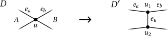
Figure 10: How to make a 3-edge-connected distillation $D$ cubic by edge expansion, Case 1: If $u$ is a cutvertex, make sure that the new edge $e_{u}$ is a chord of a cycle.

We now argue that $D^{\prime}$ is 3-edge-connected. A bond in $D^{\prime}$ which does not involve $e_{u}$ is obviously a bond in $D$, so any 1- or 2-bond in $D^{\prime}$ would include $e_{u}$, since $D$ is 3-edge-connected. In $D^{\prime}$, $e_{u}$ is a chord of the cycle $C_{a}\cup C_{b}$, so $e_{u}$ is not a 1-bond and $D^{\prime}$ is bridgeless. Consider $D^{\prime}-e_{u}$. Deleting a chord does not change the block structure and so $D^{\prime}-e_{u}$ is also bridgeless. This implies that $D^{\prime}$ is 3-edge-connected.

Case 2: $u$ is not a cutvertex. Expanding an edge $e_{u}=u_{1}u_{2}$ at $u$ so that both $u_{1}$ and $u_{2}$ have degree at least 3 can be done in several ways. Since $u$ is not a cutvertex, this surgery cannot create a bridge, but it might create a 2-bond, as in Figure 11. If it does not create a 2-bond, we are done. On the other hand, suppose that expanding the edge $e_{u}$ as above creates the 2-bond $\{e_{u},e\}$ in the resulting graph $D^{0}$.

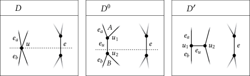
Figure 11: How to make a 3-edge-connected distillation $D$ cubic by edge expansion, Case 2: If $u$ is not a cutvertex, a 2-bond can possibly arise (as in $D^{0}$), but can also be avoided (as in $D^{\prime}$).

This implies that $u$ is a cutvertex in the graph $D-e$. Noting that $D-e$ is bridgeless, we expand a new edge $e_{u}$ in this graph, exactly as described in Case 1. Let $D^{\prime}-e$ denote the resulting graph, and then restore $e$ to obtain $D^{\prime}$. The proof that $D^{\prime}$ is 3-edge-connected follows Case 1 verbatim.

Finally, we note that in both Case 1 and Case 2, the new vertices $u_{1}$ and $u_{2}$ have degrees between 3 and $(\deg(u)-1)$, thereby lowering the average degree of the distillation. Thus, we can repeat the above procedure until we obtain a 3-edge-connected, cubic weak distillation of $G$. This proves part (a).

Proof of part (b).

If $G$ itself has no nontrivial 2-bonds, then the statement is true by part (a). Suppose on the other hand that $G$ has at least one nontrivial 2-bond, and let $a$ and $b$ denote the positive chains containing the bond. We now shift all the edges in chain $b$ to chain $a$, one by one, according to Definition 13 (if $a$ is a 1-chain, use an endvertex of $a$ when expanding an edge into the chain). We call the resulting graph $G^{\prime}$, which is equivalent to $G$ by Definition 14.

Now, $G^{\prime}$ has one less positive chain. Hence, repeating the above procedure for any remaining 2-bond in $G^{\prime}$, the process eventually terminates, and we obtain a graph $G^{\dagger}\!$ which is equivalent to $G$ and whose only 2-bonds are trivial. $G^{\dagger}\!$ is bridgeless since $G$ is. By part (a), this proves part (b).

Proof of part (c).

Given $G$ and an equivalent graph $G^{\dagger}\!$ with a weak distillation $D\in\mathcal{D}_{k}$, we prove the contrapositive statement, namely that if $G^{\dagger}\!$ is balanced or has only positive chains with respect to $D$, then $G$ has a weak distillation in $\mathcal{D}_{k}$. There are two cases to consider.

Case 1: $G^{\dagger}\!$ has only positive chains relative to $D$. This implies that $D$ is the proper distillation of $G^{\dagger}\!$. Since $D$ is 3-edge-connected and cubic, it is easy to see that only trivial edge shifts can be performed in $G^{\dagger}\!$ (which means that every edge can only be shifted within its chain; see the discussion below Definition 13). Hence, $G^{\dagger}\!$ is the only graph in its equivalence class and so $G$ and $G^{\dagger}\!$ are isomorphic.

Case 2: $G^{\dagger}\!$ is balanced but has zero chains relative to $D$. This implies that every chain of $G^{\dagger}\!$ has either length one or zero. Suppose that there is a nontrivial way to shift an edge $e$ in $G^{\dagger}\!$, otherwise there is nothing to prove. We first expand an edge $e^{\prime}$ so that $\{e,e^{\prime}\}$ is a nontrivial 2-bond in the resulting graph $H$. We claim that $\{e,e^{\prime}\}$ is the only 2-bond of $H$. To see this, note that $G^{\dagger}\!$ is 3-edge connected, since $D$ is, and hence any 2-bond of $H$ necessarily involves $e^{\prime}$. But if $e^{\prime\prime}$ is some third edge such that $\{e^{\prime},e^{\prime\prime}\}$ were a 2-bond in $H$, then also the symmetric difference between $\{e,e^{\prime}\}$ and $\{e^{\prime},e^{\prime\prime}\}$ would be a 2-bond in $H$ (since it would be a cut and since $H$ is bridgeless). This would then be a 2-bond without $e^{\prime}$, giving a contradiction.

Let $H^{\prime}$ be the graph, equivalent to $G^{\dagger}\!$, which is obtained by contracting $e$ in $H$. Since $H$ has only one 2-bond, $H^{\prime}$ is 3-edge-connected, and so $H^{\prime}$ has a weak distillation $D^{\prime}$ in $\mathcal{D}_{k}$ by part (a). Since $H$ has no chains with more than one edge, the same holds for $H^{\prime}$, and hence $H^{\prime}$ is balanced with respect to $D^{\prime}$. Furthermore, $H^{\prime}$ has a zero chain relative to $D^{\prime}$, since it has a vertex of degree at least four from the contraction of $e$. It follows that every graph which is equivalent to $G^{\dagger}\!$, which in particular includes $G$, has a weak distillation in $\mathcal{D}_{k}$. ∎

6 Minimizing 2-disconnections and 3-disconnections

6.1 Minimizing 2-disconnections for $k\geq 1$

Necessary and sufficient conditions for $(n,m)$-graphs to minimize $d_{2}$ have been known since [Bauer], at least in the context of simple graphs. Our framework allows for a unified formulation with a shorter proof. The second part of the theorem describes a particular surgery which yields a lower $d_{2}$-value, and will be used repeatedly in what follows.

Theorem 6.1.

(1) For $k\geq 1$, a graph $G\in\mathcal{G}_{n,n+k}$ minimizes $d_{2}({\mkern 2.0mu\cdot\mkern 2.0mu})$ if and only if $G$ is a balanced weak subdivision of some $D\in\mathcal{D}_{k}$ (“weak” is not needed when $n\geq 2k$).

(2) If $G$ is an imbalanced weak subdivision of $D\in\mathcal{D}_{k}$, then a strictly $d_{2}$-decreasing surgery is to choose a pair of imbalanced chains and move one edge from the longer to the shorter chain.

Proof.

The proof of the only if direction of (1) will also prove (2). We suppose that $G$ is not a balanced weak subdivision of a distillation in $\mathcal{D}_{k}$ and show that $G$ does not minimize $d_{2}$. There are two cases:

Case 1: $G$ is not a weak subdivision of any graph in $\mathcal{D}_{k}$. By Theorem 5.2(a), $G$ has a bridge or $G$ is bridgeless but has nontrivial 2-bond. If $G$ has a bridge, then by Proposition 2.3 there exists a $G^{\prime}\in\mathcal{G}_{n,n+k}$ such that $d_{2}(G^{\prime})<d_{2}(G)$. If $G$ is bridgeless but has a nontrivial 2-bond, then by Theorem 5.2(b) there is an equivalent graph $G^{\dagger}\!$ with a weak distillation in $\mathcal{D}_{k}$, and by part (c), $G^{\dagger}\!$ is imbalanced with respect to this weak distillation. Since $d_{2}(G^{\dagger}\!)=d_{2}(G)$ by Proposition 5.1, we can conclude, through Case 2 below, that $G$ is not $d_{2}$-minimizing.

Case 2: $G$ is an imbalanced weak subdivision of some $D\in\mathcal{D}_{k}$. Let $a$ and $b$ be the lengths of two imbalanced chains of $G$, relative to $D$, such that $a>b+1$, and let $G^{\prime}$ be the graph obtained by moving one edge from the $a$-chain to the $b$-chain. Since $G$ and $G^{\prime}$ has only trivial 2-bonds, $d_{2}(G)$, as well as $d_{2}(G^{\prime})$, is just the number of edge-pairs where both edges are in the same chain. Thus, we obtain

$$d_{2}(G)-d_{2}(G^{\prime})=\binom{a}{2}+\binom{b}{2}-\binom{a-1}{2}-\binom{b+1}{2}\,,$$ (8)

which expands to $\frac{1}{2}\big{(}a(a-1)+b(b-1)-(a-1)(a-2)-(b+1)b\big{)}$ and simplifies to $a-(b+1)$, which is positive by our assumption on $a$ and $b$. This proves the only if direction of (1), as well as (2).

For the if direction, using the only if direction, it suffices to show that the $d_{2}$-value is the same for any $G\in\mathcal{G}_{n,n+k}$ which is a balanced weak subdivision of any graph $D\in\mathcal{D}_{k}$. $G$ has $3k$ balanced chains relative to $D$. We write $m=3kq+r$ where $0\leq r<3k$, meaning that the “base length” of the $3k$ chains is $q$, while $r$ of the chains are one unit longer (cf. (9) below). Since $d_{2}(G)$ is just the number of ways to choose two edges from some chain of $G$, we have

$$d_{2}(G)=(3k-r)\binom{q}{2}+r\binom{q+1}{2}\,.\qed$$

6.2 A result about 3-disconnections for $k\geq 2$

wangIn addition to the indication following this footnote, the closely related paper [Wang94]—apparently the single other paper written by the corresponding author of [Wang97]—contains material which is demonstrably wrong (see Section 9 below), including its main result, which we call the $K_{3,3}$-theorem. Both of these papers suffer from a similar lack of clarity and rigor.

A general statement about minimizing the number of 3-disconnections can be found in [Wang97]; however, we cannot consider this article reliable, for multiple reasons.wang The proof of a result we would need [Wang97, Theorem 10(c)] mistakenly relies on a particular picture and lacks a coherently structured argument. We will instead prove the similar Proposition 6.2 in this section, for which we need some new notation.

Consider a balanced weak $(m-k,m)$-graph which is a weak subdivision of a cubic distillation $D$. This distillation necessarily has $3k$ edges, so the $m$ edges of $G$ are distributed as evenly as possible over $3k$ chains. We wish to define a “standard length” $q\geq 0$, such that at least half of the chains of $G$ have length $q$. Using Euclidean division with a “centered remainder”, we define $q$ and $r$ according to

$$m=3kq+r\quad\mathrlap{(-3k/2<r\leq 3k/2)\,.}$$ (9)

Then, $G$ has $3k-|r|$ chains of length $q$, and the remaining $|r|$ chains have length $q-1$ if $r$ is negative and length $q+1$ if $r$ is positive.

Definition 16 ($\pi^{\kern-0.38847pt\mathrm{v}}({\mkern 2.0mu\cdot\mkern 2.0mu})$, $b_{3}^{\mathrm{v}}({\mkern 2.0mu\cdot\mkern 2.0mu})$; v stands for “vertex”).

Given a cubic, 2-edge-connected distillation $D$ with exceedance $k$, construct a balanced weak subdivision $G\in\mathcal{G}_{m-k,m}$ and assign edge weights to $D$ according to the chain lengths of $G$ (edges contracted in the construction are assigned weight 0). With $q$ given by (9), we then define the following.

1. The $\pi^{\kern-0.38847pt\mathrm{v}}\kern-0.55496pt$-value of a vertex $u_{i}\in D$, denoted $\pi^{\kern-0.38847pt\mathrm{v}}(u_{i})$, is the number of edges incident to $u_{i}$ which do not have weight $q$, counted with sign, in that the weight $q+1$ is counted positively and $q-1$ negatively. The $\pi^{\kern-0.38847pt\mathrm{v}}$-values of $D$ yield a multiset denoted by $[\pi^{\kern-0.38847pt\mathrm{v}}_{i}]_{i=1}^{2k}$. The $\pi^{\kern-0.38847pt\mathrm{v}}$-values are balanced if the maximum pairwise difference of its values is one.

2. Let $b_{3}^{\mathrm{v}}(u)$ denote the product of the weights incident to $u\in D$ (which equals the number of 3-bonds of $G$ which isolate the vertex $u$ in $D$).

Proposition 6.2.

Let $m>k\geq 2$. Given a distillation $D\in\mathcal{D}_{k}$ with only trivial 3-bonds, construct a balanced weak subdivision $G\in\mathcal{G}_{m-k,m}$ and let the edges of $D$ be weighted accordingly. Let $\mathcal{B}_{m}\subset\mathcal{G}_{m-k,m}$ contain the balanced weak subdivisions of $D$.

1. If the $\pi^{\kern-0.38847pt\mathrm{v}}$-values of $D$ are balanced, then $G$ minimizes $d_{3}({\mkern 2.0mu\cdot\mkern 2.0mu})$ in $\mathcal{B}_{m}$.

2. If $m\geq 2k$, then $G$ minimizes  $d_{3}({\mkern 2.0mu\cdot\mkern 2.0mu})$ in $\mathcal{B}_{m}$ if and only if the $\pi^{\kern-0.38847pt\mathrm{v}}$-values are balanced.

Proof.

Recall that $D$ has $2k$ vertices since $D$ is cubic; we label them $u_{i}$, where $i\in[1\mathrel{{.}\,{.}}\nobreak 2k]$. Fix $m$, which determines $r$ and $q$ according to (9). Note that if $r=0$, then there is only one balanced weak subdivision of $D$ in $\mathcal{B}_{m}$, the $\pi^{\kern-0.38847pt\mathrm{v}}$-multiset is all zeros, and the proposition is trivial. Now, construct an arbitrary balanced weak subdivision $G\in\mathcal{G}_{m-k,m}$ and assign edge weights to $D$ accordingly.

Since $D$ is 3-edge-connected, every 3-disconnection of $G$ is either a 3-bond or contains a trivial 2-bond. For every chain of length $\ell$, there are $\binom{\ell}{2}(m-\ell)$ disconnections of the latter kind. Since $G$ is balanced, the chain lengths are given, and we have

$$d_{3}(G)=K+b_{3}(G)\,,$$ (10)

where $K$ does not depend upon the choice of $G$ (nor on $D$), and $b_{3}(G)$ is the number of 3-bonds of $G$. Since all 3-bonds of $D$ are trivial, all 3-bonds of $G$ are. Hence,

$$b_{3}(G)=\sum_{\mathclap{i\in[1\mathrel{{.}\,{.}}\nobreak 2k]}}b_{3}^{\mathrm{v}}(u_{i})\,,$$ (11)

where the possible values of $b_{3}^{\mathrm{v}}(u)$ are given in Table 1.

$\pi^{\kern-0.38847pt\mathrm{v}}(u)$		$\mathrlap{b_{3}^{\mathrm{v}}(u)}$	$\varphi_{3}(\pi^{\kern-0.38847pt\mathrm{v}})$
$0$	$\phantom{(q\pm 1)^{2}}q^{3}$	${}=q^{3}$	$0$
$\pm 1$	$(q\pm 1)^{1}q^{2}$	${}=q^{3}\pm q^{2}$	$0$
$\pm 2$	$(q\pm 1)^{2}q^{1}$	${}=q^{3}\pm 2q^{2}+q$	$q$
$\pm 3$	$(q\pm 1)^{3}$	${}=q^{3}\pm 3q^{2}+3q\pm 1$	$3q\pm 1$

Table 1: Functions for counting and comparing the number of trivial 3-bonds in balanced weak subdivisions of cubic, 3-edge-connected graphs.

Now, considering (11) and the values of $b_{3}^{\mathrm{v}}$ in the table, we see that $b_{3}(G)$ is a cubic polynomial in $q$, and that the leading coefficient is $2k$. We also assert that the coefficient of the quadratic term always equals $2r$. To see this, first note that $\pi^{\kern-0.38847pt\mathrm{v}}(u_{i})$ has the same sign as $r$, and then consider that there are $|r|$ edges in $D$ which are potentially counted by $\pi^{\kern-0.38847pt\mathrm{v}}(u_{i})$. As $u_{i}$ ranges over the vertices of $D$, each of these edges is counted twice. This implies that

$$\sum_{\mathclap{i\in[1\mathrel{{.}\,{.}}\nobreak 2k]}}\pi^{\kern-0.38847pt\mathrm{v}}(u_{i})=2r\,.$$ (12)

The assertion now follows by noting that the quadratic coefficient of $b_{3}^{\mathrm{v}}(u)$ equals $\pi^{\kern-0.38847pt\mathrm{v}}(u)$ in each row of the table.

Let $\varphi(\pi^{\kern-0.38847pt\mathrm{v}})$—also denoted by $\varphi_{3}(\pi^{\kern-0.38847pt\mathrm{v}})$, see Table 1—be the constant and linear terms of $b_{3}^{\mathrm{v}}$ regarded as a function of $\pi^{\kern-0.38847pt\mathrm{v}}\kern-0.55496pt$. Combining the above observations about $b_{3}(G)$ with (10) yields

$$d_{3}(G)=K+2kq^{3}+2rq^{2}+\sum_{\mathclap{i\in[1\mathrel{{.}\,{.}}\nobreak 2k]}}\varphi(\pi^{\kern-0.38847pt\mathrm{v}}_{i})\,,$$ (13)

where only $\pi^{\kern-0.38847pt\mathrm{v}}_{i}\mathrel{\vbox{\hbox{\scriptsize.}\hbox{\scriptsize.}}}=\pi^{\kern-0.38847pt\mathrm{v}}(u_{i})$ depends upon the choice of $G$. Hence, $G$ minimizes $d_{3}$ within our class if and only if $G$ minimizes $\sum_{i}\varphi(\pi^{\kern-0.38847pt\mathrm{v}}_{i})$.

Using Table 1, it is easy to verify the following three pairs of inequalities. 1: $\varphi(0)+\varphi(\pm 2)\geq 2\varphi(\pm 1)$, 2: $\varphi(0)+\varphi(\pm 3)\geq\varphi(\pm 2)+\varphi(\pm 1)$, 3: $\varphi(\pm 1)+\varphi(\pm 3)\geq 2\varphi(\pm 2)$. (Recall that the $\pm$ signs correspond to whether $r$ is positive or negative, and if $r=0$ the inequalities do not apply.) The inequalities imply that the sum $\sum_{i}\varphi(\pi^{\kern-0.38847pt\mathrm{v}}_{i})$ is bounded below by the value of the sum if the $\pi^{\kern-0.38847pt\mathrm{v}}_{i}$’s were replaced by a balanced multiset also satisfying (12). This implies part (1) of the proposition.

Proof of (2). In view of (1), we need only show the only if direction. This is accomplished by proving the following two statements, given $m\geq 2k$. A: Of the a priori possible $\pi^{\kern-0.38847pt\mathrm{v}}$-multisets, which satisfy (12), only the balanced one minimizes $\sum_{i}\varphi(\pi^{\kern-0.38847pt\mathrm{v}}_{i})$. B: There exists a $(m-k,m)$-graph which induces a balanced $\pi^{\kern-0.38847pt\mathrm{v}}$-multiset in $D$.

Statement A would follow immediately if all the three inequalities 1, 2 and 3 above were strict. This is close to being true. We first restrict to the case where $m\geq 3k$. This implies that $q\geq 2$ or that $q=1$ and $r\geq 0$, and then all the inequalities are strict (if $r\neq 0$ so that they apply; otherwise, recall that the proposition is trivial).

The remaining case is when $2k\leq m<3k$, which implies $q=1$ and $r\in[-k\mathrel{{.}\,{.}}\nobreak-1]$. The positive $q$-value guarantees that the first two inequalities are strict. To see that this suffices to prove A, consider the following: The multiset sums to $2r$ and so has mean value $r/k$, which implies that a balanced $\pi^{\kern-0.38847pt\mathrm{v}}$-multiset in this case only contains the numbers $-1$ and $0$. Hence, if step by step changing an imbalanced multiset into the balanced one, either inequality 1 or 2 will need to be applied at the last step.

We now prove B. The distillation $D$ is bridgeless and cubic since $D\in\mathcal{D}_{k}$, and so by Petersen’s Theorem [Diestel, Cor. 2.2.2] there is a perfect matching in $D$. Let $E_{1}$ denote the $k$ edges of a perfect matching (recall Lemma 2.1) and let $E_{2}$ denote the remaining $2k$ edges of $D$.

With this, we can specify how to weigh the edges of $D$ to obtain balanced $\pi^{\kern-0.38847pt\mathrm{v}}$-values and an implied weak subdivision $G$. We start by assigning weight $q$ to all edges; we will then change $r$ edges to either weight $q-1$ or $q+1$. Care must be taken so that we do not create a cycle with all zero weights, since this is not compatible with the definition of a weak subdivision. This concern arises when $2k\leq m<3k$, so that $q=1$ and $r\in[-k\mathrel{{.}\,{.}}\nobreak-1]$. Otherwise, things are analogous for positive and for negative $r$, and we therefore suppose that $r$ is negative.

If on the one hand $r\in[-k\mathrel{{.}\,{.}}\nobreak-1]$, let the $r$ edges with weight $q-1$ be arbitrarily chosen from $E_{1}$. Since these edges are independent, each vertex of $D$ is incident with at most one edge with weight $q-1$, and so the $\pi^{\kern-0.38847pt\mathrm{v}}$-multiset contains only the values $-1$ and $0$. There is no cycle of edges weighted $q-1$, and hence we have specified a weak subdivision of $D$.

If on the other hand $r\in[\lceil-3k/2\rceil\mathrel{{.}\,{.}}\nobreak k-1]$, we start by assigning weight $q-1$ to the $k$ edges of the perfect matching $E_{1}$, which guarantees that each $\pi^{\kern-0.38847pt\mathrm{v}}$-value is at least $-1$. We now need to assign weight $q-1$ to another $|r|-k\leq\lceil k/2\rceil$ edges in such a way that no vertex obtains $\pi^{\kern-0.38847pt\mathrm{v}}$-value $-3$. This is equivalent to choosing a matching of size $|r|-k$ in $E_{2}$. The graph $E_{2}$ is 2-regular, and is hence a union of cycles; each with at least three edges since $D$ is simple, and with a total number of $2k$ edges. This makes it is immediate that $E_{2}$ has a matching of size $\lceil k/2\rceil$, and hence a matching of size $|r|-k$, as required. ∎

Corollary 6.3 (of the above proof).

Let $k\geq 2$ and $m\geq 3k$ and consider the set of all balanced subdivisions, with $m$ edges, of all graphs in $\mathcal{D}_{k}$. Within this set, $G$ minimizes $d_{3}({\mkern 2.0mu\cdot\mkern 2.0mu})$ if and only if its proper distillation $D\in\mathcal{D}_{k}$ has only trivial 3-bonds and balanced $\pi^{\kern-0.38847pt\mathrm{v}}$-values with respect to $G$ (the latter condition is vacuous when $3k\mathrel{\mid}\nobreak m$).

Proof.

After noting that there always exist a graph in $\mathcal{D}_{k}$ with only trivial 3-bonds—consider the $k$-Möbius ladder of Definition 17—we can re-use the previous proof, with a minor modification and addition.

As noted, (10) holds for any balanced weak $(m-k,m)$-subdivision $G$ of any graph in $D\in\mathcal{D}_{k}$, where $K$ does not depend on $G$ nor $D$. However, (11) as well as (13), has to be modified by adding a term accounting for the number of nontrivial 3-bonds of $G$, which we may denote by $b_{3}^{\mathrm{n}}(G)$. By combining a few terms in (13) and adding $b_{3}^{\mathrm{n}}(G)$, we obtain

$$d_{3}(G)=K^{\prime}+\Phi(G)+b_{3}^{\mathrm{n}}(G)\,,$$ (14)

where $K^{\prime}$ denotes the first three terms of (13), which depend neither on $G$ nor on $D$, and $\Phi(G)$ denotes the “$\varphi$-sum” which depends only upon the $\pi^{\kern-0.38847pt\mathrm{v}}$-multiset. With no further modifications, the preceding proof shows that a balanced $\pi^{\kern-0.38847pt\mathrm{v}}$-multiset is sufficient, and necessary if $m\geq 2k$, for $\Phi(G)$ to be minimized.

Now suppose that $m\geq 3k$, so that $G$, being balanced, has only positive chains relative to $D$, which is to say that $D=D_{G}$. Clearly, $G$ has a nontrivial 3-bond if and only if $D_{G}$ has a nontrivial 3-bond (see Lemma 3.2). It follows that $d_{3}(G)$ is minimized, within the set under consideration, if and only if its proper distillation has balanced $\pi^{\kern-0.38847pt\mathrm{v}}$-values w.r.t. $G$ and no nontrivial 3-bonds. ∎

Remark.

Corollary 6.3 could be extended to hold for $m\geq 2k$ (with a weak replacing its proper) if the following were true, which would be a natural extension of Theorem 5.2(a). (The only if direction is easy.)

Question. Let, for $k\geq 2$, $G$ be a bridgeless graph in $\mathcal{G}_{n,n+k}$. Is it true that $G$ has a weak distillation in $\mathcal{D}_{k}$ with only trivial 3-bonds if and only if all 2-bonds and 3-bonds of $G$ are trivial?

7 Moving edges between chains

We will often want to move an edge from a longer chain to a shorter chain and study how the number of disconnecting sets of a certain size, say $i$, changes. Suppose that we obtain $G^{\prime}$ from $G$ by moving an edge between chains. In principle, it would be straightforward to compare $c_{i}(G^{\prime})$ and $c_{i}(G)$. Each term in $c_{i}({\mkern 2.0mu\cdot\mkern 2.0mu})$ is a product of $i$ chain lengths (cf. (6)) and corresponds to a connected spanning subgraph of $D_{G}$ where $i$ edges are missing. However, the expressions become impractical, and the calculations do not seem very helpful to the intuition. It is possible to instead obtain a formula for $d_{i}(G)-d_{i}(G^{\prime})$ directly by inspection, without first obtaining full expressions for $c_{i}(G)$ or $d_{i}(G)$ and $c_{i}(G^{\prime})$ or $d_{i}(G^{\prime})$. The idea is that only edge sets which disconnect exactly one of the two graphs contribute to the above difference. Necessary and sufficient conditions for edge sets to have this property are laid out in Lemma 7.1, and the practical application is in Corollary 7.2. (The proof of the lemma follows after the corollary.) The reader might want to skip directly to Example 8.1 for a demonstration.

Lemma 7.1.

Let $G$ be a connected graph, and let $G^{\prime}$ be obtained from $G$ by moving an edge $e$, i.e. contract $e$ and then expand an edge at some vertex in the graph, which we also call $e$. Identify the edges of $G$ with the edges of $G^{\prime}$ in the natural way. Then an edge set $E$ disconnects $G$ but not $G^{\prime}$ if and only if $E$ satisfies both of the following conditions.

1. In $G$, $E$ contains exactly one bond $B$, and $e\in B$.

2. In $G^{\prime}$, there is no bond $F$ such that $e\in F\subseteq E$.

Remark.

If condition (1) of the lemma holds, then (2) is equivalent to the following simpler, but less practically useful, condition: (2$\,{}^{\prime}\!$) $E$ does not disconnect $G^{\prime}$.

Corollary 7.2.

Let $G^{\prime}$ be obtained from $G$ as in the preceding lemma. For $i\in[1\mathrel{{.}\,{.}}\nobreak m]$ and $1\leq j\leq i$, let $x_{i,j}$ be the number of edge sets of size $i$, which fulfill conditions (1) and (2) above, and where the bond $B$ has size $j$. Let $x^{\prime}_{i,j}$ be the corresponding number of edge sets, but with the roles of $G$ and $G^{\prime}$ interchanged in conditions (1) and (2). Then

$$d_{i}(G)-d_{i}(G^{\prime})=\sum_{j=1}^{i}x_{i,j}-x^{\prime}_{i,j}\,,\quad\mathrlap{\forall i\in[1\mathrel{{.}\,{.}}\nobreak m]\,.}$$ (15)

Proof of Corollary 7.2.

The unprimed terms in the right-hand side of (15) sum to the number of edge sets of size $i$ which disconnect $G$ but not $G^{\prime}$, and vice versa for the primed terms. ∎

Proof of Lemma 7.1.

Let $G$, $G^{\prime}$, and $E$ be as in the statement of the lemma. We exhaust the possibilities for the set $E$, and show for each case that the two sides of the biconditional (if and only if) statement of the lemma either both hold or both fail.

Case 1: $E$ does not disconnect $G$. It is immediate that neither side of the biconditional holds.

Case 2: $E$ contains a bond $B$ in $G$ such that $e\notin B$. Then $B$ is a bond also in $G/e=G^{\prime}/e$, and thus $B$ is a bond in $G^{\prime}$. Again, both sides of the biconditional fail.

Case 3: $E$ contains exactly one bond $B$ in $G$, and $e\in B$. By interchanging $G$ and $G^{\prime}$ in the reasoning of Case 2, we see that if $E$ contains a bond $F$ in $G^{\prime}$, then such a bond necessarily contains $e$. If there is such a bond $F$ in $G^{\prime}$, both sides of the biconditional fail. If there is no such bond, then both sides hold.

Note that if $E$ contains two bonds in $G$, both of which include $e$, then the symmetric difference of these bonds is a cut $C$, which does not include $e$. This is covered by Case 2, and thus, the possibilities are exhausted. ∎

8 The uniquely optimal $(k=2)$-graphs

multiconfusionThere is some confusion in the literature about which arguments and results apply only to simple graphs and which apply also to graphs with multiple edges. Although it seems that the intention of Boesch, Li and Suffel [Li] was to cover multigraphs, Gross and Saccoman [Gross] are nevertheless credited in the literature with extending their main result from simple graphs to multigraphs, by way of a separate argument.

We are now equipped to consider the sets of $(n,n+2)$-graphs. The description of the optimal graphs of these sets (for $n$ at least $4$ or $5$) has been published in several places; see [Li], [Tseng] and [Wu], and is rephrased below in Theorem 8.3. The description is in three parts, corresponding to the three steps below, and hence any treatment showing these graphs to be uniquely optimal or UMRGs should reasonably contain the following:

1. Identification of $K_{4}$ as the relevant distillation.

2. Proof that a $K_{4}$-subdivision has to be balanced to be possibly $p$-optimal.

3. Specification of how longer or shorter chains need to be arranged, in case the chain lengths are not exactly the same.

Compared to the other presentations, our treatment has the following advantages. Firstly, Step 1 requires no additional work within our framework, but follows as Proposition 8.2. Secondly, due to flaws described in the following paragraphs, Step 2, which corresponds to our Proposition 8.1, has never before been given a correct, direct proof. (An implicit proof using Tutte polynomials was just recently found by [Tutte].) Lastly, graphs with multiple edges and loops need no separate arguments.multiconfusion We note that this naturally gives results starting for $n=1$.

The main result of [Li] is [Li, Theorem 4], which indirectly identifies the $(n,n+2)$-UMRGs for $n\geq 5$. The proof of this theorem has a serious flaw. The middle part of the proof aims to show what we identify as Step 2, or more precisely, that a $K_{4}$-subdivision has to be balanced in order to maximize the number of spanning trees. The authors argue that, given any two chains $\ell_{a}$ and $\ell_{b}$ in such a graph for which $\ell_{a}-\ell_{b}\geq 2$, a graph with strictly more spanning trees is obtained by moving an edge from $\ell_{a}$ to $\ell_{b}$. However, this claim is false, as shown by Example 8.1 below. (In addition, one of the four 2-connected proper distillations of $(n,n+2)$-graphs, shown in Figure 5, is missing from the analysis in [Li].)

With regard to [Tseng] and [Wu], both papers justify Step 2 by stating the solution of the corresponding constrained optimization problem for continuous variables. While we are open to the possibility of a proof in this direction, it is not clear to us how the integer-valued solution follows (except when they coincide).

Example 8.1.

This example provides an infinite set of counterexamples to a mistaken deduction in [Li] which implies Step 2. In the process, we derive (17), which we then use to properly prove Step 2 (see Proposition 8.1). We focus on one particular counterexample, from which an infinite set is then easily obtained.

The false statement in [Li] is that if $(\ell_{a},\ell_{b})$ is an imbalanced pair of chains of a $K_{4}$-subdivision, then the graph obtained by moving one edge from the longer to the shorter chain has strictly more spanning trees. Let $G$ be a subdivision of $K_{4}$, according to Figure 12, with chain lengths $(\ell_{1},\ell_{2},\allowbreak\ell_{3},\allowbreak\ell_{4},\allowbreak\ell_{5},\ell_{6})=\allowbreak(3,3,\allowbreak 1,\allowbreak 1,\allowbreak 1,5)$, and let $G^{\prime}$ be the graph obtained by moving an edge $e$ from $\ell_{1}$ to $\ell_{3}$. We use Corollary 7.2 to show that $d_{3}(G)-d_{3}(G^{\prime})=-1$, which is to say that $G^{\prime}$ has one less spanning tree than $G$.

Figure 12: $G$ is a subdivision of $K_{4}$, and $G^{\prime}$ is obtained from $G$ by moving an edge from a longer to a shorter chain. Thus, the latter graph is “more balanced”, but nonetheless it has one less spanning tree.

Neither $G$ nor $G^{\prime}$ has bonds of size 1. Therefore, by Corollary 7.2,

$$d_{3}(G)-d_{3}(G^{\prime})=x_{3,2}-x^{\prime}_{3,2}+x_{3,3}-x^{\prime}_{3,3}\,.$$ (16)

We explain in detail how to explicitly obtain the first term of this expression. In effect, $x_{3,2}$ counts the number of $3$-sets $E_{3}$ which disconnect $G$ by a 2-bond, but do not disconnect $G^{\prime}$. In $G$, an edge in $\ell_{1}$ should be a priori chosen as $e$, the first edge of $E_{3}$. We then count the number of ways to choose two more edges for $E_{3}$. WLOG, the second edge and $e$ should form a 2-bond (condition 1) so $e_{2}$ could be any one of the remaining $\ell_{1}-1$ edges in the same chain. The third edge, $e_{3}$, should not cause $E_{3}$ to contain any other bond in $G$ (also condition 1) which precludes $e_{3}\in\ell_{1}$. Nor should $E_{3}$ contain any bond in $G^{\prime}$, which would then necessarily contain $e$. This is condition 2, which precludes $e_{3}\in\ell_{3}$ (which would create a 2-bond in $G^{\prime}$) and $e_{3}\in\ell_{5}$ (which would create a 3-bond in $G^{\prime}$). Thus, the possible choices for $e_{3}$ are the edges in $\ell_{2}$, $\ell_{4}$ and $\ell_{6}$.

Hence, we obtain $x_{3,2}=(\ell_{1}-1)(\ell_{2}+\ell_{4}+\ell_{6})$. Similarly, $x^{\prime}_{3,2}=\ell_{3}(\ell_{2}+\ell_{4}+\ell_{6})$, $x_{3,3}=\ell_{6}\ell_{4}$ and $x^{\prime}_{3,3}=\ell_{6}\ell_{2}$. Insertion into (16) yields

$$d_{3}(G)-d_{3}(G^{\prime})=(\ell_{1}-1-\ell_{3})(\ell_{2}+\ell_{4}+\ell_{6})+(\ell_{4}-\ell_{2})\ell_{6}\,.$$ (17)

With the given chain lengths, this sums to $-1$. From (17) it is immediate that one could instead start with any $K_{4}$-subdivision for which $\ell_{1}-\ell_{3}=2$ and the other chains have the same lengths as in $G$, and obtain the exact same result.

Proposition 8.1.

Let $G\in\mathcal{G}_{n,n+2}$, where $n\geq 1$. If $G$ is an imbalanced weak subdivision of $K_{4}$, then there is another weak subdivision $H\in\mathcal{G}_{n,n+2}$ of $K_{4}$ such that $d_{2}(H)<d_{2}(G)$ and $d_{3}(H)<d_{3}(G)$. Hence, an imbalanced weak $K_{4}$-subdivision can never be $p$-optimal.

Proof.

Let $G\in\mathcal{G}_{n,n+2}$ be a weak subdivision of $K_{4}$ with imbalanced chains. We label the chains $\ell_{1}$ through $\ell_{6}$ according to Figure 13. Suppose that $\ell_{1}$ and $\ell_{3}$ have the largest difference in length among all pairs of chains which are $K_{4}$-adjacent and that $\ell_{1}$ is chosen as large as possible with this condition. In particular, we have $\ell_{1}>\ell_{3}$, and we define $\delta\mathrel{\vbox{\hbox{\scriptsize.}\hbox{\scriptsize.}}}=\ell_{1}-\ell_{3}$.

Figure 13: A general representation of a subdivision of $K_{4}$. The edges represent chains, and the $\ell_{i}$-labels are chain lengths. We can also regard the lengths as weights on the edges of $K_{4}$.

Let $G^{\prime}$ be the graph obtained by moving one edge from $\ell_{1}$ to $\ell_{3}$, which gives another weak subdivision of $K_{4}$ in $\mathcal{G}_{n,n+2}$. Let $\Delta\mathrel{\vbox{\hbox{\scriptsize.}\hbox{\scriptsize.}}}=d_{3}(G)-d_{3}(G^{\prime})$, a formula for which was obtained in Example 8.1 using Corollary 7.2. Rearranging (17) gives

$$\begin{split}\Delta&=(\delta-1)(\ell_{2}+\ell_{4}+\ell_{6})-\ell_{6}(\ell_{2}-\ell_{4})\\ &=(\delta-1)(\ell_{2}+\ell_{4})+\ell_{6}((\delta-1)-(\ell_{2}-\ell_{4}))\,.\end{split}$$ (18)

Our main task is to prove that $\Delta$, in general, is positive. However, In three particular cases, $\Delta$ will be zero, which says that $G$ and $G^{\prime}$ has the same number of spanning trees. In these three cases, we will repeat the same surgery on $G^{\prime}$ to obtain $G^{\prime\prime}$, which will have strictly more spanning trees than $G^{\prime}$ and $G$.

Case 1: $\delta=1$. In this case, we must have $\ell_{1}=a+2$, $\ell_{2}=a$, and $\ell_{3}=\ell_{4}=\ell_{5}=\ell_{6}=a+1$, for some $a$. We obtain

$$\Delta=-\ell_{6}(\ell_{2}-\ell_{4})=-(a+1)\left(a-(a+1)\right)=a+1\geq 1\,.$$

Case 2: $\delta\geq 2$ and $\ell_{2}-\ell_{4}=\delta$. Insertion into (18) gives

$$\begin{split}\Delta&=(\delta-1)((\delta+\ell_{4})+\ell_{4})-\ell_{6}\\ &=(\delta-2)(\delta+2\ell_{4})+\ell_{4}+(\delta-(\ell_{6}-\ell_{4}))\geq 0\,,\end{split}$$

since all three terms are nonnegative.

We consider the possibility of $\Delta$ being $0$. This is when all three terms of the expression are zero, i.e. $\delta=2$, $\ell_{4}=0$ and $\ell_{6}-\ell_{4}=\delta$, which implies $\ell_{6}=2$. Since also $\ell_{2}-\ell_{4}=\delta$, we also have $\ell_{2}=2$. Furthermore, our assumption that $\ell_{1}-\ell_{3}=\delta$ is the largest possible difference between adjacent chains forces $\ell_{1}$ to be $2$ (since $\ell_{1}$ is adjacent to a zero chain) and $\ell_{3}$ to be $0$. Lastly, since $\ell_{5}$ is also adjacent to a zero chain, $\ell_{5}\leq 2$. Thus, the chains of $G$ are $(\ell_{1},\ldots,\ell_{6})=(2,2,0,0,[0\text{ or }1\text{ or }2],2)$. In each of these three cases, $G^{\prime}$ is an imbalanced graph distinct from the three described above. Starting from the beginning with $G^{\prime}$ instead of $G$ will give a graph $G^{\prime\prime}$ with strictly lower $d_{3}$-value. (In fact, $G^{\prime}$ will fall into Case 3.)

Case 3: $\delta\geq 2$ and $\ell_{2}-\ell_{4}\leq\delta-1$. We first assume that at least one of $\ell_{2}$ and $\ell_{4}$ is positive. Then, insertion into the last part of (18) gives $\Delta\geq(\delta-1)(\ell_{2}+\ell_{4})>0$. If on the other hand $\ell_{2}=\ell_{4}=0$, insertion into (18) gives $\Delta=\ell_{6}(\delta-1)$. To see that this has to be positive, consider that $G$ is obtained from $K_{4}$ by exchanging every edge for a chain. When $\ell_{2}$ and $\ell_{4}$ are replaced by zero chains, they are contracted. Since $\ell_{2}$, $\ell_{4}$ and $\ell_{6}$ correspond to a cycle in $K_{4}$, $\ell_{6}$ is positive since “zero cycles” are impossible, so $\Delta>0$.

Now let either $H\mathrel{\vbox{\hbox{\scriptsize.}\hbox{\scriptsize.}}}=G^{\prime}$, or for any of the three exceptional cases, $H\mathrel{\vbox{\hbox{\scriptsize.}\hbox{\scriptsize.}}}=G^{\prime\prime}$. We have shown that $H$ is a weak $K_{4}$-subdivision in $\mathcal{G}_{n,n+2}$ with a lower $d_{3}$-value than $G$. By the second part of Theorem 6.1, $H$ has also a strictly lower $d_{2}$-value. Hence, by (3) in Section 2.2, $R(H,p)>R(G,p)$ for all $p$. ∎

Proposition 8.2.

Let $G\in\mathcal{G}_{n,n+2}$, where $n\geq 1$. If $G$ is not a weak subdivision of $K_{4}$, then there is a graph $H\in\mathcal{G}_{n,n+2}$ such that $d_{3}(H)<d_{3}(G)$ and $d_{2}(H)<d_{2}(G)$. Hence, any $p$-optimal $(n,n+2)$-graph is a weak distillation of $K_{4}$.

Proof.

Let $G\in\mathcal{G}_{n,n+2}$, where $n\geq 1$, and suppose that $G$ is not a weak subdivision of $K_{4}$. If $G$ has a bridge, the statement follows from Proposition 2.3, so we can assume $G$ to be bridgeless. From Theorem 5.2 it follows that $G$ is equivalent to some weak subdivision $G^{\dagger}\!$ of $K_{4}$ (being the only distillation in $\mathcal{D}_{2}$) and that $G^{\dagger}\!$ is imbalanced with respect to $K_{4}$. Since $G$ and $G^{\dagger}\!$ have the same reliability function (Proposition 5.1), the statement follows directly from Proposition 8.1. ∎

The only thing remaining for a complete description of the family of optimal $(n,n+2)$-graphs, is to consider different arrangements of longer and shorter chains, among $K_{4}$-subdivisions, when the number of edges is not divisible by six. This is accomplished by Theorem 8.3. The first nine uniquely optimal $(n,n+2)$-graphs are illustrated in Figure 14.

Theorem 8.3.

For each $n\geq 1$ and $m=n+2$, there is a uniquely optimal graph in $\mathcal{G}_{n,m}$. This graph is a balanced weak subdivision of $K_{4}$ (“weak” is not needed when $n\geq 4$), which is specified up to isomorphism by the following set of additional conditions, where $m\equiv r\pmod{6}$ and $r\in[-2\mathrel{{.}\,{.}}\nobreak 3]$.

• If $r\in\{0,\pm 1\}$, no further condition is needed.

• If $r=2$ ($r=-2$), the two longer (shorter) chains correspond to a matching in $K_{4}$.

• If $r=3$, the three longer chains correspond to a simple 3-path in $K_{4}$.

Figure 14: The first ten uniquely optimal $(n,n+2)$-graphs. The pattern continues and cycles every six graphs.

Remark.

The following characterization due to [Li] generates the uniquely optimal $(n,n+2)$-graphs for $n\geq 4$: Cycle through the three perfect matchings of $K_{4}$ and successively introduce a new vertex into each of the corresponding chains.

Proof.

Fix $n\geq 1$, so $m\geq 3$, and consider the subset of $\mathcal{G}_{n,m}$ which contains the balanced weak subdivisions of $K_{4}$. Since $m$ is fixed, $r\in[-2\mathrel{{.}\,{.}}\nobreak 3]$ is fixed; see (9). If $r=0$, all chains have the same length, so we have a single perfectly balanced graph. There is also only one graph when $r=\pm 1$, since $K_{4}$ is edge-transitive.

In the other cases, $G$ minimizes $d_{3}({\mkern 2.0mu\cdot\mkern 2.0mu})$ within our subset if and only if $G$ induces balanced $\pi^{\kern-0.38847pt\mathrm{v}}$-values in $K_{4}$, according to Proposition 6.2 (except for the only if direction when $m=3$, but in this case there is only one graph, the 3-bouquet).

Suppose that $r=2$ ($r=-2$). There are then two possible choices for $G$: The two longer (shorter) chains can either be adjacent or nonadjacent, and this choice specifies $G$ up to isomorphism. Only the latter choice, which corresponds to a perfect matching in $K_{4}$, gives a balanced $\pi^{\kern-0.38847pt\mathrm{v}}$-multiset, namely $[\pi^{\kern-0.38847pt\mathrm{v}}_{i}]_{i=1}^{4}=[1]_{i=1}^{4}$ (or $[-1]_{i=1}^{4}$, respectively).

Suppose that $r=3$. There are exactly three nonisomorphic graphs which can be obtained from different arrangements of the three longer chains, except for when $m=3$. The options are as follows. The longer chains can either A: emanate from one vertex, B: form a cycle, or C: form a simple path. Only option C gives a balanced $\pi^{\kern-0.38847pt\mathrm{v}}$-multiset, namely $[\pi^{\kern-0.38847pt\mathrm{v}}_{i}]_{i=1}^{4}=[1,2,2,1]$. (This option is well-defined also for $m=3$, since the shorter chains do not form a cycle.)

We now use Proposition 8.2 and 8.1 to conclude that the specified graph uniquely minimizes $d_{3}({\mkern 2.0mu\cdot\mkern 2.0mu})$ over the entire set $\mathcal{G}_{n,m}$. By Theorem 6.1 it also minimizes $d_{2}({\mkern 2.0mu\cdot\mkern 2.0mu})$. Unique optimality follows. ∎

9 The uniquely optimal $(k=3)$-graphs

9.1 Background

mobiusThe four first Möbius ladders are included in Figure 9. If Conjecture LABEL:con.wagnerLABEL:wagnerconj, concerning $(k=4)$-graphs holds, then for each $k\in\{1,2,3,4\}$, all the $p$-optimal $(n,n+k)$-graphs are weak subdivisions of the $k$-Möbius ladder. But considering $k=5$, the Petersen graph is a UMRG, and is manifestly not a weak subdivision of $M_{5}$.

To find the most reliable graphs with exceedance 3, we need to study weak subdivisions of the two graphs in $\mathcal{D}_{3}$, namely the triangular prism $\Pi_{3}$ and the complete bipartite graph $K_{3,3}$ (also known as the utility graph). The former graph is the focus of Section 9.2. Regarding the latter, $K_{3,3}$, its two most common representations are shown in Figure 15. While representation A most clearly displays the bipartite structure, representation B indicates that $K_{3,3}$ belongs to the Möbius ladders, defined below.mobius

Figure 15: Two representations of the complete bipartite graph $K_{3,3}$.

Definition 17.

For $k\geq 1$, the $k$-Möbius ladder, denoted by $M_{k}$, is the graph obtained from $C_{2k}$ by adding an edge between each pair of opposite vertices. The $2k$ edges in the cycle are rails and the $k$ additional edges are rungs (but note that $M_{k}$ is edge transitive for $k\in\{1,2,3\}$), and we extend this terminology to chains in weak subdivisions of $M_{k}$.

$K_{3,3}$ is similar to $K_{4}$ in that its edge set can be partitioned into three perfect matchings. Recall from the remark after Theorem 8.3 that the sequence of uniquely optimal $(n,n+2)$-graphs can be generated by a rule involving the perfect matchings of $K_{4}$. For this and other reasons, Boesch, Li and Suffel [Li] conjectured that UMRGs could be similarly generated from $K_{3,3}$ as follows:

Partition the nine edges of $K_{3,3}$ into three perfect matchings. Cycle through these matchings and successively introduce a new vertex into each of the corresponding chains.

This conjecture has been considered a theorem since 1994, when Wang [Wang94] published a proof of what he called Boesch’s Conjecture. This result has been cited more than 50 times, without any indication of a mistake being detected. However, as we show in Section 9.4, this theorem is false. Our treatment is independent to that of [Wang94], which in addition to reaching the wrong conclusion about $K_{3,3}$-subdivisions also has fatal flaw in its treatment of $\Pi_{3}$-subdivisions, as we will demonstrate in Example 9.1.

9.2 Subdivisions of the triangular prism are not $p$-optimal

Consider $\Pi_{3}$ with the edges labeled as in Figure 16. Regarding $\Pi_{3}$ as a “circular ladder”, we call the $c$-edges rungs and the $l$- and $r$-edges rails; and we call two rails with the same index corresponding rails. Note that $K_{3,3}$, being a Möbius ladder, can be obtained from the circular ladder $\Pi_{3}$ by introducing a “half-twist”, or more precisely, by exchanging the incidences of two rails $l_{i}$ and $r_{i}$ across one of the two adjacent rungs $c_{j}$, as shown in Figure 16. With the labels interpreted as chain lengths, this surgery is a reconnection of the chains $l_{i}$ and $r_{i}$ across $c_{j}$.

Figure 16: The triangular prism $\Pi_{3}$ (left). Reconnecting $l_{1}$ and $r_{1}$ across $c_{1}$ gives $K_{3,3}$ (right). The edge labels can be interpreted as chain lengths (yielding weak subdivisions of $\Pi_{3}$ and $K_{3,3}$) or as weights representing such lengths.

Theorem 9 in [Wang94] says that any $(n,n+3)$-graph which maximizes the number of spanning trees must have $K_{3,3}$ as its proper distillation. This is indeed true for $n\geq 6$; however, the proof given by Wang is incorrect. The proof claims to show by induction that given a $\Pi_{3}$-subdivision $G$, then the graph obtained by reconnecting two corresponding rail chains has strictly more spanning trees. In contradiction to this, there exists an infinite number of $\Pi_{3}$-subdivisions for which every $K_{3,3}$-subdivision with the same chain lengths has strictly less spanning trees, as shown in Example 9.1. In Proposition 9.2 we show that a subdivision of $\Pi_{3}$ cannot maximize the number of spanning trees nor be $p$-optimal for any $p$.

Example 9.1.

smithThis can be seen by inspecting the A-representation of Figure 15 and is equivalent to the fact that the line graph of $K_{3,3}$ is distance transitive with diameter two [Smith].

This example gives an infinite family of “strong” counterexamples to the central claim of the proof of [Wang94, Theorem 9], namely that if $G$ is a subdivision of $\Pi_{3}$, and $G^{\prime}$ is the $K_{3,3}$-subdivision obtained by reconnecting two corresponding rail chains of $G$, as in Figure 16, then $G^{\prime}$ has more spanning trees than $G$. Our counterexamples are strong in the sense that for any graph in the family, every possible rearrangement of chains into a $K_{3,3}$-subdivision has less spanning trees. We focus on a particular such example, and then indicate its generalization.

Our particular example is the graph $G$ in Figure 17, which is a subdivision of $\Pi_{3}$, and has 50 more spanning trees than $G^{\prime}$ and 2 more than $G^{\prime\prime}$. The latter two graphs are the only subdivisions $K_{3,3}$ with the same chain lengths as $G$, which follows from the fact that up to isomorphism, there is only one way to choose two adjacent edges of $K_{3,3}$ and only one way to choose two nonadjacent edges.smith

Figure 17: A subdivision of $\Pi_{3}$, $G$, which has more spanning threes than the $K_{3,3}$-subdivisions $G^{\prime}$ and $G^{\prime\prime}$, with the same chain lengths. This was previously claimed impossible.

The first part of the claim amounts to $d_{4}(G)=d_{4}(G^{\prime})-50=d_{4}(G^{\prime\prime})-2$. To show this, we write

$$d_{4}({\mkern 2.0mu\cdot\mkern 2.0mu})=d_{4,2}({\mkern 2.0mu\cdot\mkern 2.0mu})+d_{4,3}({\mkern 2.0mu\cdot\mkern 2.0mu})+d_{4,4}({\mkern 2.0mu\cdot\mkern 2.0mu})\,,$$ (19)

where $d_{4,i}({\mkern 2.0mu\cdot\mkern 2.0mu})$ is the number of 4-disconnections in which the smallest bond has size $i$. Regarding $d_{4,2}({\mkern 2.0mu\cdot\mkern 2.0mu})$, it is easy to see that the number of edge sets of size 4 (or of any given size) which contain a 2-bond is the same for the three graphs: Pair up the chains of $G$ with those of $G^{\prime}$ (or $G^{\prime\prime}$) by length, and consider an induced pairing between the edges. Thus, $G$, $G^{\prime}$ and $G^{\prime\prime}$ have the same $d_{4,2}$-value.

It is not hard to calculate $d_{4,3}$ and $d_{4,4}$ for the three graphs; we start with $d_{4,4}$. Every 4-bond of $\Pi_{3}$ and $K_{3,3}$ is trivial (isolates one edge), and by Corollary 3.3, interpreting chains as weighted edges, we go through the chains of $G$, $G^{\prime}$ and $G^{\prime\prime}$, multiply the adjacent chain lengths, and sum the results to obtain

$$d_{4,4}(G) = 5^{2}1^{2}+6\cdot 5^{1}1^{3}+2\cdot 1^{4}=57$$

$$d_{4,4}(G^{\prime}) = 5^{2}1^{2}+6\cdot 5^{1}1^{3}+2\cdot 1^{4}=57$$

$$d_{4,4}(G^{\prime\prime}) =2\cdot{} 5^{2}1^{2}+4\cdot 5^{1}1^{3}+3\cdot 1^{4}=73$$

Regarding $d_{4,3}$, we note that $G^{\prime}$ and $G^{\prime\prime}$ have only trivial 3-bonds, while $G$ in addition has a nontrivial 3-bond which separates the two 3-cycles. Any edge set counted by $d_{4,3}$ is obtained in the following way (see Lemma 3.2): (1) Choose a 3-bond in the proper distillation (2) Pick one edge from each of the corresponding chains (3) Choose a fourth edge from any one of the other 6 chains; this does not create any additional bond. This gives

$$d_{4,3}(G) = 4\cdot 5^{1}1^{2}10+3\cdot 1^{3}14=242$$

$$d_{4,3}(G^{\prime}) =5^{2}1^{1}6+{} 2\cdot 5^{1}1^{2}10+3\cdot 1^{3}14=292$$

$$d_{4,3}(G^{\prime\prime}) = 4\cdot 5^{1}1^{2}10+2\cdot 1^{3}14=228$$

Comparing the numbers above, it is clear that both $G^{\prime}$ and $G^{\prime\prime}$ have a higher number of 4-disconnections than $G$. In particular, with obvious shorthand, $d_{4}^{\prime}-d_{4}=292-242=50$ and $d_{4}^{\prime\prime}-d_{4}=(73-57)+(228-242)=2$.

Finally, replacing the two chains of length 5 by two chains which are at least as long gives us an infinite number of similar examples.

In what follows, we will use the below notation to simplify the algebra. Let

$$\delta_{i}\mathrel{\vbox{\hbox{\scriptsize.}\hbox{\scriptsize.}}}=l_{i}-r_{i}\quad\textrm{and}\quad\sigma_{i}\mathrel{\vbox{\hbox{\scriptsize.}\hbox{\scriptsize.}}}=l_{i}+r_{i}\,,$$ (20)

where $i\in\{1,2,3\}$, and $l_{i}$ and $r_{i}$ refer to chain lengths of $\Pi_{3}$, according to Figure 16.

Lemma 9.1.

Considering Figure 16, let $G$ be a weak subdivision of $\Pi_{3}$ in which all $c_{i}$’s are positive. Suppose that (1) $\delta_{1}\geq 1$, (2) $-\delta_{3}>\delta_{2}\geq 0$ and (3) $\max(\delta_{1},-\delta_{3})>1$, referring to (20). Then there is another weak subdivision $G^{\prime\prime}$ of $\Pi_{3}$, obtained by moving two edges between $l_{i}$- and $r_{i}$-chains, such that $d_{i}(G^{\prime\prime})<d_{i}(G)$ for $i\in\{2,3,4\}$.

Proof.

Let $G$ be a weak subdivision of $\Pi_{3}$, with chains labeled according to $\Pi_{3}$ in Figure 16, fulfilling (1), (2) and (3), and with positive $c$-chains. We obtain $G^{\prime\prime}\in\mathcal{G}_{n,n+3}$ from $G$ by first moving one edge from the $l_{1}$-chain to the $r_{1}$-chain, calling the intermediate graph $G^{\prime}$, and then moving one edge from the $r_{3}$-chain to the $l_{3}$-chain; see Figure 18. These surgeries are possible since $l_{1}\geq l_{1}-r_{1}\geq 1$ by (1) and $r_{3}\geq r_{3}-l_{3}\geq 1$ by (2). Clearly, $G^{\prime\prime}$ is a weak subdivision of $\Pi_{3}$.

Figure 18: $G$ is a weak subdivision of $\Pi_{3}$. An edge $e\in G$ is moved to obtain $G^{\prime}$, in which another edge $e^{\prime}$ is moved to obtain $G^{\prime\prime}$ (not shown).

We use the shorthand $d_{i}$ for $d_{i}(G)$, with primes added for $G^{\prime}$ and $G^{\prime\prime}$. By Theorem 6.1 we have $d_{2}^{\prime\prime}<d_{2}$, since we have twice moved an edge from a longer to a shorter chain, and at least one of these two chain pairs was initially imbalanced, by the assumption $\max(l_{1}-r_{1},r_{3}-l_{3})>1$.

Let $C\mathrel{\vbox{\hbox{\scriptsize.}\hbox{\scriptsize.}}}=c_{1}+c_{2}+c_{3}$. Through Corollary 7.2, since $G$ and $G^{\prime}$ are bridgeless, we obtain

$$d_{3}-{}d_{3}^{\prime} =x_{3,2}-x_{3,2}^{\prime}+x_{3,3}-x_{3,3}^{\prime}$$

$$=(l_{1}-1)(C+\sigma_{2}+\sigma_{3})-r_{1}(C+\sigma_{2}+\sigma_{3})+(c_{1}l_{2}+c_{3}l_{3})-(c_{1}r_{2}+c_{3}r_{3})$$

$$=(\delta_{1}-1)(c_{1}+c_{2}+c_{3}+\sigma_{2}+\sigma_{3})+c_{1}\delta_{2}+c_{3}\delta_{3}\,.$$ (21)

Now, we can make appropriate substitutions in (9.2), according to Figure 18, to obtain

$$d_{3}^{\prime}-d_{3}^{\prime\prime}=(-\delta_{3}-1)(c_{1}+c_{2}+c_{3}+\sigma_{1}+\sigma_{2})+c_{3}(-\delta_{1}+2)+c_{2}(-\delta_{2})\,.$$

Adding the two equations above yields, with some rearranging and canceling,

$$\begin{multlined}d_{3}-d_{3}^{\prime\prime}=(\delta_{1}-1)(c_{1}+c_{2}+\sigma_{2}+\sigma_{3})\\ +(-\delta_{3}-1)(c_{1}+\sigma_{1}+\sigma_{2})+c_{1}\delta_{2}+c_{2}(-\delta_{3}-1-\delta_{2})\,.\end{multlined}d_{3}-d_{3}^{\prime\prime}=(\delta_{1}-1)(c_{1}+c_{2}+\sigma_{2}+\sigma_{3})\\ +(-\delta_{3}-1)(c_{1}+\sigma_{1}+\sigma_{2})+c_{1}\delta_{2}+c_{2}(-\delta_{3}-1-\delta_{2})\,.$$ (22)

We claim that all four terms above are nonnegative, and that at least one is positive. We have already noted that $c_{1}>0$. By the assumptions on $\delta_{1}$ and $\delta_{3}$, we have $\delta_{1}\geq 1$ and $-\delta_{3}\geq 1$, with at least one strict inequality. Thus, the first two terms are nonnegative and at least one is positive. The third term is nonnegative since $\delta_{2}\geq 0$, and the fourth since $-\delta_{3}-1\geq\delta_{2}$. Hence $d_{3}(G^{\prime\prime})<d_{3}(G)$.

Finally, we study how the number of 4-disconnections changes. Corollary 7.2 gives

$$d_{4}-d_{4}^{\prime}=(x_{4,2}-x_{4,2}^{\prime})+(x_{4,3}-x_{4,3}^{\prime})+(x_{4,4}-x_{4,4}^{\prime})\,.$$ (23)

We calculate the three terms above. The first two are similar to what was done in (9.2). Letting $C_{\times}\mathrel{\vbox{\hbox{\scriptsize.}\hbox{\scriptsize.}}}=c_{1}c_{2}+c_{1}c_{3}+c_{2}c_{3}$, one can verify the following. Except for in the $(l_{1}-1)$ term, all minus signs below come from the subtracted primed $x$-terms, and there is no cancellation involved.

$$x_{4,2}-x_{4,2}^{\prime} =\big{(}(l_{1}-1)-r_{1}\big{)}\big{(}C_{\times}+c_{1}\sigma_{3}+c_{3}\sigma_{2}+c_{2}(\sigma_{2}+\sigma_{3})+\sigma_{2}\sigma_{3}\big{)}$$

$$x_{4,3}-x_{4,3}^{\prime} =c_{1}(l_{2}-r_{2})(c_{2}+c_{3}+\sigma_{3})+c_{3}(l_{3}-r_{3})(c_{1}+c_{2}+\sigma_{2})$$ (24)

$$x_{4,4}-x_{4,4}^{\prime} =c_{1}c_{2}(l_{3}-r_{3})+c_{3}c_{2}(l_{2}-r_{2})$$

We add these three equations, using (20). (The five colors will soon be explained.) This yields

$$\begin{multlined}d_{4}-d_{4}^{\prime}=(\delta_{1}-1)({\color[rgb]{.804,0,0}C_{\times}}+c_{1}\sigma_{3}+{\color[rgb]{0,.545,0}c_{3}\sigma_{2}}+c_{2}(\sigma_{2}+\sigma_{3})+\sigma_{2}\sigma_{3})\\ +c_{1}\delta_{2}({\color[rgb]{.545,.46,0}c_{2}}+{\color[rgb]{.545,.28,.536}c_{3}}+\sigma_{3})+c_{3}\delta_{3}({\color[rgb]{.804,0,0}c_{1}+c_{2}}+{\color[rgb]{0,.545,0}\sigma_{2}})+{\color[rgb]{.804,0,0}c_{1}c_{2}\delta_{3}}+{\color[rgb]{0,0,.804}c_{3}c_{2}\delta_{2}}\,.\end{multlined}d_{4}-d_{4}^{\prime}=(\delta_{1}-1)({\color[rgb]{.804,0,0}C_{\times}}+c_{1}\sigma_{3}+{\color[rgb]{0,.545,0}c_{3}\sigma_{2}}+c_{2}(\sigma_{2}+\sigma_{3})+\sigma_{2}\sigma_{3})\\ +c_{1}\delta_{2}({\color[rgb]{.545,.46,0}c_{2}}+{\color[rgb]{.545,.28,.536}c_{3}}+\sigma_{3})+c_{3}\delta_{3}({\color[rgb]{.804,0,0}c_{1}+c_{2}}+{\color[rgb]{0,.545,0}\sigma_{2}})+{\color[rgb]{.804,0,0}c_{1}c_{2}\delta_{3}}+{\color[rgb]{0,0,.804}c_{3}c_{2}\delta_{2}}\,.$$ (25)

We obtain $d_{4}^{\prime}-d_{4}^{\prime\prime}$ by making substitutions in (25) according to Figure 18:

$$\begin{multlined}d_{4}^{\prime}-d_{4}^{\prime\prime}=(-\delta_{3}-1)({\color[rgb]{.804,0,0}C_{\times}}+{\color[rgb]{0,.545,0}c_{3}\sigma_{2}}+c_{2}\sigma_{1}+c_{1}(\sigma_{1}+\sigma_{2})+\sigma_{1}\sigma_{2})\\ +c_{3}(-\delta_{1}+2)({\color[rgb]{.804,0,0}c_{1}+c_{2}}+{\color[rgb]{0,.545,0}\sigma_{2}})+c_{2}(-\delta_{2})({\color[rgb]{0,0,.804}c_{3}}+{\color[rgb]{.545,.46,0}c_{1}}+\sigma_{1})+{\color[rgb]{.545,.28,.536}c_{3}c_{1}(-\delta_{2})}+{\color[rgb]{.804,0,0}c_{2}c_{1}(-\delta_{1}+2)}\,.\end{multlined}d_{4}^{\prime}-d_{4}^{\prime\prime}=(-\delta_{3}-1)({\color[rgb]{.804,0,0}C_{\times}}+{\color[rgb]{0,.545,0}c_{3}\sigma_{2}}+c_{2}\sigma_{1}+c_{1}(\sigma_{1}+\sigma_{2})+\sigma_{1}\sigma_{2})\\ +c_{3}(-\delta_{1}+2)({\color[rgb]{.804,0,0}c_{1}+c_{2}}+{\color[rgb]{0,.545,0}\sigma_{2}})+c_{2}(-\delta_{2})({\color[rgb]{0,0,.804}c_{3}}+{\color[rgb]{.545,.46,0}c_{1}}+\sigma_{1})+{\color[rgb]{.545,.28,.536}c_{3}c_{1}(-\delta_{2})}+{\color[rgb]{.804,0,0}c_{2}c_{1}(-\delta_{1}+2)}\,.$$

Now, adding the last two equations, all the same-colored terms cancel. We obtain

$$\begin{split}d_{4}-d_{4}^{\prime\prime}={}&(\delta_{1}-1)(c_{1}\sigma_{3}+c_{2}(\sigma_{2}+\sigma_{3})+\sigma_{2}\sigma_{3})+c_{1}\delta_{2}\sigma_{3}\\ &+(-\delta_{3}-1)(c_{2}\sigma_{1}+c_{1}(\sigma_{1}+\sigma_{2})+\sigma_{1}\sigma_{2})-c_{2}\delta_{2}\sigma_{1}\,,\end{split}$$

and with a slight rearrangement in the second line

$$\begin{split}d_{4}-d_{4}^{\prime\prime}={}&(\delta_{1}-1)(c_{1}\sigma_{3}+c_{2}(\sigma_{2}+\sigma_{3})+\sigma_{2}\sigma_{3})+c_{1}\delta_{2}\sigma_{3}\\ &+(-\delta_{3}-1)\big{(}c_{1}(\sigma_{1}+\sigma_{2})+\sigma_{1}\sigma_{2}\big{)}+c_{2}\sigma_{1}(-\delta_{3}-1-\delta_{2})\,.\end{split}$$ (26)

Again, we claim that all four terms above are nonnegative, and that at least one is positive, for almost exactly the same reasons as for (22). The only additional observation needed is that $\sigma_{1}\geq 1$ and $\sigma_{3}\geq 1$, since $\delta_{1}\geq 1$ and $-\delta_{3}\geq 1$. With this, we can conclude that the first or the third term is positive, and hence that $d_{4}(G^{\prime\prime})<d_{4}(G)$. ∎

Proposition 9.2.

For $n\geq 2$, let $G\in\mathcal{G}_{n,n+3}$ be a weak subdivision of $\Pi_{3}$ which is not also a weak subdivision of $K_{3,3}$ (equivalently, in which the three $c$-chains in Figure 16 are positive). Then there is a weak $K_{3,3}$-subdivision $G^{\prime}\in\mathcal{G}_{n,n+3}$ such that $d_{2}(G^{\prime})\leq d_{2}(G)$, $d_{3}(G^{\prime})<d_{3}(G)$ and $d_{4}(G^{\prime})<d_{4}(G)$, and so $G^{\prime}$ is strictly more reliable than $G$. (In particular, a subdivision of $\Pi_{3}$ cannot be $p$-optimal for any value of $p$.)

Proof.

Fix $n\geq 2$ and let $G\in\mathcal{G}_{n,n+3}$ be a weak subdivision of $\Pi_{3}$, which is not also a weak subdivision of $K_{3,3}$. Importantly, this implies that the chains which correspond to the nontrivial 3-bond of $\Pi_{3}$ are positive. (Otherwise $G$ would be a weak subdivision of both $\Pi_{3}$ and $K_{3,3}$, since the two graphs in Figure 16 become isomorphic when contracting any of the $c$-edges.)

We first consider a particular degenerate case. The graph $\Pi_{3}$ has two 3-cycles. If, for either one of these cycles, two out of the three corresponding chains of $G$ are zero chains, then the third chain is a cycle with a cutvertex. (Recall that all chains in a cycle cannot be zero.) Suppose that $G$ is such a graph and WLOG that $r_{1}$ is a cycle, as shown in Figure 19, where also one or two of the $l$-chains, but no other chains, are allowed to be zero.

Figure 19: A weak $\Pi_{3}$-subdivision $G$ in which the chain $r_{1}$ is a cycle, and a strictly more reliable graph $G^{\prime}$, obtained by reconnecting one incidence of $r_{1}$ to an endvertex of an adjacent chain.

We construct $G^{\prime}$ by moving one incidence of $r_{1}$ to an endvertex of an $l$-chain. No calculations are required to observe that $d_{2}(G^{\prime})=d_{2}(G)$, that $d_{3}(G^{\prime})<d_{3}(G)$ and that $d_{4}(G^{\prime})<d_{4}(G)$; just note that every edge set which disconnects $G^{\prime}$ also disconnects $G$, but that there are edge sets of size 3 and 4 (which contain an edge from each of the $c_{i}$’s) that disconnect $G$ but not $G^{\prime}$. (This argument is easily generalizable to any graph with a “loop chain”.) Furthermore, contracting two nonadjacent edges of $K_{3,3}$ yields $K_{4}$ with a double edge, so, comparing with Figure 19, we note that $G^{\prime}$ is actually a weak subdivision of $K_{3,3}$.

The more general possibility which remains is that $G$ has at most one zero chain for each 3-cycle of $\Pi_{3}$. Suppose henceforth that $G$ is such a graph, and label the chains as in Figure 16 and according to the following restrictions. R1: At least two of the values $\delta_{1}$, $\delta_{2}$ and $\delta_{3}$, see (20), should be nonnegative. R2: If one or two of the $\delta_{i}$-values are zero, then the nonnegative numbers should include the largest of the three absolute values. R3: $\delta_{1}\geq\delta_{2}\geq\delta_{3}$. (R1 and R2 can be satisfied by appropriately choosing the “left” and “right” sides of $G$, while R3 is satisfied by an appropriate indexing.) Note that $\delta_{1}\geq\delta_{2}\geq 0$ by R1 and R3. Also note that if $\delta_{3}$ is negative, then $\delta_{1}$ is forced to be positive by R2. Now, there are three cases.

Case 1: $\delta_{3}<-\delta_{2}$ and $\max(\delta_{1},-\delta_{3})>1$. We claim that the conditions of Lemma 9.1 are then fulfilled. We only need to verify conditions (1) and (2). Since $\delta_{2}\geq 0$ by R2, we have that $\delta_{3}$ is negative. As noted earlier, this implies that $\delta_{1}$ is positive, which is condition (1). Also, $\delta_{2}$ is nonnegative by R1, so $-\delta_{3}>\delta_{2}\geq 0$, which is (2). Thus, by Lemma 9.1, there is a weak $\Pi_{3}$-subdivision $H\in\mathcal{G}_{n,n+3}$ with unchanged $c$-chains and strictly smaller $d_{i}$-values than $G$ has, for $i\in\{2,3,4\}$. By relabeling the chains of $H$ according to R1, R2 and R3, and if necessary repeatedly applying this Lemma 9.1, we eventually obtain a graph which falls into Case 2 or Case 3. The surgery explained in Case 3 will then finally give us the desired graph $G^{\prime}$.

Case 2: $\delta_{3}<-\delta_{2}$ and $\max(\delta_{1},-\delta_{3})\leq 1$. Then, just as in Case 1, $\delta_{1}$ is positive, $\delta_{2}$ is nonnegative and $\delta_{3}$ is negative. But then $\max(\delta_{1},-\delta_{3})\leq 1$ implies that $\delta_{1}=-\delta_{3}=1$, and since $-\delta_{3}>\delta_{2}$ it follows from R3 that $\delta_{2}=0$. Thus $(\delta_{1},\delta_{2},\delta_{3})=(1,0,-1)$. We finish Case 2 after Case 3.

Case 3: $\delta_{3}\geq-\delta_{2}$. By considering different cases, one can check that at least one of the pairs $\{l_{1},r_{1}\}$ and $\{l_{2},r_{2}\}$ must consist of positive chains. We obtain $G^{\prime}\in\mathcal{G}_{n,n+3}$ from $G$ by either reconnecting the chains $l_{1}$ and $r_{1}$ (if they are both positive) or the chains $l_{2}$ and $r_{2}$ (if they are both positive) across $c_{1}$, as shown in Figure 16. If both surgeries are possible, they yield the same graph. Since the chain lengths are unchanged by the surgery, we have that $d_{2}(G^{\prime})=d_{2}(G)$.

We now follow a method similar to what was done in Example 9.1. Since the chain lengths are the same, the number of 3- and 4-disconnections which contain a 2-bond is the same for $G$ as for $G^{\prime}$. In particular, to obtain $d_{3}(G)-d_{3}(G^{\prime})$ we only need to compare the number of 3-bonds $b_{3}(G)$ and $b_{3}(G^{\prime})$. By Corollary 3.3, we can use the 3-bonds of the correspondingly edge-weighted graphs $\Pi_{3}$ and $K_{3,3}$. These distillations have the same 3-bonds, except for the trivial bonds which separate an endvertex of $c_{1}$ from the rest of the graph, and for the nontrivial bond $\{c_{1},c_{2},c_{3}\}$ of $\Pi_{3}$; see Figure 16. Thus, using Corollary 3.3,

$$d_{3}-d_{3}^{\prime}=b_{3}-b_{3}^{\prime} =c_{1}c_{2}c_{3}+c_{1}l_{1}l_{2}+c_{1}r_{1}r_{2}-c_{1}r_{1}l_{2}-c_{1}l_{1}r_{2}$$ (27)

$$=c_{1}\big{(}c_{2}c_{3}+(l_{1}-r_{1})(l_{2}-r_{2})\big{)}=c_{1}(c_{2}c_{3}+\delta_{1}\delta_{2})\,.$$

This expression is positive since the $c_{i}$’s are positive and since $\delta_{1}$ and $\delta_{2}$ are nonnegative. Hence, $d_{3}(G^{\prime})<d_{3}(G)$.

Furthermore, to obtain $d_{4}(G)-d_{4}(G^{\prime})$, we use the notation of (19) in Example 9.1 and write

$$d_{4}(G)-d_{4}(G^{\prime})=d_{4,3}(G)-d_{4,3}(G^{\prime})+d_{4,4}(G)-d_{4,4}(G^{\prime})\,,$$ (28)

where $d_{4,i}({\mkern 2.0mu\cdot\mkern 2.0mu})$ is the number of 4-disconnections in which the smallest bond is an $i$-bond. We have also used the fact that $d_{4,2}({\mkern 2.0mu\cdot\mkern 2.0mu})$ is unchanged.

We start with $d_{4,3}(G)-d_{4,3}(G^{\prime})$. The 3-bonds of $G$ and $G^{\prime}$ which are not counted in (27) are in a natural one-one correspondence, which induces a one-one correspondence between the 4-disconnections which contain any of these bonds. We deduce that any 4-disconnection without a 2-bond, and which is not in the aforementioned one-one correspondence, is obtained by choosing some 3-bond counted in $b_{3}(G)-b_{3}(G^{\prime})$, see (27), and adding an edge from a fourth chain. Thus,

$$\begin{split}d_{4,3}-d_{4,3}^{\prime}={}&c_{1}\big{(}c_{2}c_{3}(\sigma_{1}+\sigma_{2}+\sigma_{3})+l_{1}l_{2}({\color[rgb]{.804,0,0}r_{1}+r_{2}}+c_{2}+c_{3}+\sigma_{3})+r_{1}r_{2}({\color[rgb]{.804,0,0}l_{1}+l_{2}}+c_{2}\\ &+c_{3}+\sigma_{3})-r_{1}l_{2}({\color[rgb]{.804,0,0}l_{1}+r_{2}}+c_{2}+c_{3}+\sigma_{3})-l_{1}r_{2}({\color[rgb]{.804,0,0}l_{2}+r_{1}}+c_{2}+c_{3}+\sigma_{3})\big{)}\end{split}$$

$$={} c_{1}\big{(}c_{2}c_{3}(\sigma_{1}+\sigma_{2}+\sigma_{3})+(l_{1}-r_{1})(l_{2}-r_{2})(c_{2}+c_{3}+\sigma_{3})\big{)}\,,$$ (29)

where the terms in red cancel (because every edge set which contains one edge each from four out of the five chains in $\{c_{1},l_{1},l_{2},r_{1},r_{2}\}$ disconnects both $G$ and $G^{\prime}$).

To obtain $d_{4,4}(G)-d_{4,4}(G^{\prime})$, we use that every 4-bond in $\Pi_{3}$ and $K_{3,3}$, and hence in $G$ and $G^{\prime}$, is trivial. Furthermore, every labeled edge in the two distillations has the same adjacencies, except for the four edges $l_{1}$, $l_{2}$, $r_{1}$ and $r_{2}$; see Figure 16. Thus, using Corollary 3.3, we multiply the four adjacent edge-weights for each of these four edges, then sum the results for $\Pi_{3}$ (representing $G$) and subtract the results for $K_{3,3}$ (representing $G^{\prime}$). This yields

$$\begin{split}d_{4,4}-d_{4,4}^{\prime}={}&c_{1}c_{3}l_{2}l_{3}+c_{1}c_{2}l_{1}l_{3}+c_{1}c_{3}r_{2}r_{3}+c_{1}c_{2}r_{1}r_{3}\\ &-c_{1}c_{3}l_{3}r_{2}-c_{1}c_{2}l_{3}r_{1}-c_{1}c_{3}l_{2}r_{3}-c_{1}c_{2}l_{1}r_{3}\\ ={}&c_{1}c_{2}(l_{1}-r_{1})(l_{3}-r_{3})+c_{1}c_{3}(l_{2}-r_{2})(l_{3}-r_{3})\end{split}$$ (30)

Adding (9.2) and (30), according to (28), and using the notation of (20), gives us

$$d_{4}-d_{4}^{\prime\prime} =c_{1}\big{(}c_{2}c_{3}(\sigma_{1}+\sigma_{2}+\sigma_{3})+\delta_{1}\delta_{2}(c_{2}+c_{3}+\sigma_{3})+c_{2}\delta_{1}\delta_{3}+c_{3}\delta_{2}\delta_{3}\big{)}$$

$$=c_{1}\big{(}c_{2}c_{3}(\sigma_{1}+\sigma_{2}+\sigma_{3})+\delta_{1}\delta_{2}\sigma_{3}+c_{2}\delta_{1}(\delta_{2}+\delta_{3})+c_{3}\delta_{2}(\delta_{1}+\delta_{3})\big{)}\,.$$ (31)

We know that $c_{1}$ is positive, and that the four terms of the second factor are at least nonnegative: $\delta_{2}+\delta_{3}\geq 0$ since $\delta_{3}\geq-\delta_{2}$ by assumption, and then it follows from R3 that $\delta_{1}+\delta_{3}\geq 0$. Furthermore, since $c_{2}$ and $c_{3}$ are positive, and at least some $l_{i}$ or $r_{i}$ is positive, the first term is positive. Hence, $d_{4}(G^{\prime})<d_{4}(G)$.

Case 2, finished: Obtain $G^{\prime}$ from $G$ as in Case 3, and note that $d_{2}(G^{\prime})=d_{2}(G)$. Insert $(\delta_{1},\delta_{2},\delta_{3})=(1,0,-1)$ into (27) to obtain $d_{3}(G)-d_{3}(G^{\prime})=c_{1}c_{2}c_{3}>0$, and then into (9.2) to obtain $d_{4}(G)-d_{4}(G^{\prime})=c_{1}\big{(}c_{2}c_{3}(\sigma_{1}+\sigma_{2}+\sigma_{3})-c_{2}\big{)}=c_{1}c_{2}\big{(}c_{3}(\sigma_{1}+\sigma_{2}+\sigma_{3})-1\big{)}$. Since $\sigma_{1}+\sigma_{2}+\sigma_{3}\geq 4$, we conclude that $d_{4}(G)-d_{4}(G^{\prime})\geq 3c_{1}c_{2}>0$, which finishes the proof. ∎

9.3 The uniquely optimal graph is a (weak) $K_{3,3}$-subdivision

In Figure 20 we introduce a new labeling of the edges of $K_{3,3}$ (and hence of the chains of any weak subdivision of $K_{3,3}$, where we can let the labels represent chain lengths). As an edge labeling, it is useful to note that three edges share a vertex if and only if they all share the same letter or index. Furthermore, the 4-cycles are exactly the sets of edges with labels that combine two out of three letters and two out of three indices; for example, $a_{3}a_{1}c_{1}c_{3}$ specifies a 4-cycle in $K_{3,3}$.

Figure 20: $K_{3,3}$ with an edge labeling used extensively in Section 9.3. The labels can also be regarded as chain lengths for any weak subdivision of $K_{3,3}$.

With the labels of Figure 20 representing chain lengths, we let

$$\delta_{i}\mathrel{\vbox{\hbox{\scriptsize.}\hbox{\scriptsize.}}}=a_{i}-b_{i}\quad\textrm{and}\quad\sigma_{i}\mathrel{\vbox{\hbox{\scriptsize.}\hbox{\scriptsize.}}}=a_{i}+b_{i}+c_{i}\,,$$ (32)

for $i\in\{1,2,3\}$.

We will need formulas for how the number of 3- and 4-disconnections, $d_{3}({\mkern 2.0mu\cdot\mkern 2.0mu})$ and $d_{4}({\mkern 2.0mu\cdot\mkern 2.0mu})$, change when an edge is moved between adjacent chains. Let $G$ be a weak subdivision of $K_{3,3}$ with chains labeled according to Figure 20 and so that $a_{1}$ is positive, and let $G^{\prime}$ be constructed from $G$ by moving one edge from $a_{1}$ to $b_{1}$. Using Corollary 7.2, we obtain

$$d_{3}(G)-d_{3}(G^{\prime})=(\delta_{1}-1)(\sigma_{2}+\sigma_{3})+a_{2}a_{3}-b_{2}b_{3}\,,$$ (33)

where the first term originates from $x_{3,2}-x_{3,2}^{\prime}$, the second term is $x_{3,3}$ and the third is $x_{3,3}^{\prime}$. (See the derivations of the similar equations (17) and (9.2) for greater detail.) The change in the number of 4-disconnections will be obtained in the proof of Proposition 9.4.

Lemma 9.3.

Let $G$ be a weak $K_{3,3}$-subdivision, and let $a_{1}$ and $b_{1}$ be two adjacent chains which have the largest possible difference in length among all pairs of adjacent chains, relative to $K_{3,3}$. Let $G^{\prime}$ be the graph obtained by moving an edge from $a_{1}$ to $b_{1}$. If $a_{1}-b_{1}\geq 2$, then $d_{3}(G^{\prime})<d_{3}(G)$.

Proof.

Let $G$ be a weak subdivision of $K_{3,3}$ where the two adjacent chains $a_{1}$ and $b_{1}$ have the largest possible difference among all adjacent pairs, $a_{1}$ is the longer chain, and $a_{1}-b_{1}\geq 2$. Label the other chains as in Figure 20 and with the additional condition that $a_{2}-b_{2}\geq a_{3}-b_{3}$. (To see that this is always possible, take a labeling where the condition does not hold. Exchange the places of the vertices $2$ and $3$ in Figure 20 and then relabel the chains to agree with the figure.) We thus have that $\delta_{1}\geq 2$, $\delta_{1}\geq\max(|\delta_{2}|,|\delta_{3}|)$ and $\delta_{2}\geq\delta_{3}$.

Now, construct $G^{\prime}$ by moving one edge from $a_{1}$ to $b_{1}$. Let $d_{3}(G)-d_{3}(G^{\prime})\mathrel{=}\mathrel{\vbox{\hbox{\scriptsize.}\hbox{\scriptsize.}}}\Delta$. By rewriting (33) we obtain

$$\Delta =(\delta_{1}-1)(\sigma_{2}+\sigma_{3})+(a_{2}-b_{2})a_{3}+(a_{3}-b_{3})b_{2}$$

$$=(\delta_{1}-1)(c_{2}+c_{3})+(\delta_{1}-2)(a_{2}+b_{3})+(\delta_{1}+\delta_{2})a_{3}+(\delta_{1}+\delta_{3})b_{2}+(\delta_{2}-\delta_{3})$$

$$\geq(c_{2}+c_{3})+(\delta_{1}+\delta_{2})a_{3}+(\delta_{1}+\delta_{3})b_{2}+(\delta_{2}-\delta_{3})\geq 0.$$ (34)

We now only need to prove that $\Delta=0$ above is impossible. Suppose for contradiction that $\Delta=0$, which implies that all four terms in the last line above are zero. In particular $c_{2}=c_{3}=0$ and $\delta_{2}=\delta_{3}$. Let $\delta_{2,3}\mathrel{\vbox{\hbox{\scriptsize.}\hbox{\scriptsize.}}}=\delta_{2}=\delta_{3}$.

If, on the one hand, $\delta_{1}+\delta_{2,3}>0$, then, considering the second and third terms of (34), $a_{3}=b_{2}=0$. Then, $\delta_{2}=\delta_{3}$ simplifies to $a_{2}=-b_{3}$, so $a_{2}$ and $b_{3}$ are also zero chains. However, this would give us several “zero cycles”, such as $c_{2}c_{3}a_{3}a_{2}$, which is not possible for a weak subdivision.

If, on the other hand, $\delta_{1}+\delta_{2,3}=0$, then, in particular, $\delta_{1}=-\delta_{2}=b_{2}-a_{2}$, so $b_{2}=\delta_{1}+a_{2}$. Since $b_{2}$ is adjacent to the zero chain $c_{2}$, we also have $b_{2}=b_{2}-c_{2}\leq\delta_{1}$. Together, this gives $a_{2}\leq 0$, so $a_{2}$ is a zero chain. Analogously, we see that $a_{3}$ is a zero chain, which again leads to the zero cycle $c_{2}c_{3}a_{3}a_{2}$. We conclude that, necessarily, $\Delta>0$. ∎

Proposition 9.4.

If $G$ is an imbalanced weak $K_{3,3}$-subdivision, then there is a graph $G^{\prime}$, obtained by moving an edge between two adjacent chains of $G$, such that $d_{2}(G^{\prime})\leq d_{2}(G)$, $d_{3}(G^{\prime})<d_{3}(G)$ and $d_{4}(G^{\prime})<d_{4}(G)$.

Proof.

Let $G$ be an imbalanced weak subdivision of $K_{3,3}$. We will construct $G^{\prime}$ by moving an edge from one chain of $G$ to an adjacent chain. Since there is only one way to choose two adjacent edges of $K_{3,3}$ up to isomorphism (as noted in Example 9.1) we can assume that we want to move an edge from the $a_{1}$-chain to the $b_{1}$-chain of Figure 20, but without yet specifying how these chains are to be chosen.

Our first task is to obtain an expression for $d_{4}(G)-d_{4}(G^{\prime})$. This is done by Corollary 7.2. We start with the $x_{i,j}$-terms, which are obtained in the same way as for (9.2). By the corollary, we then add the three following equations together to obtain $d_{4}(G)-d_{4}(G^{\prime})$.

$$x_{4,2}-x_{4,2}^{\prime} =\big{(}(a_{1}-1)-b_{1}\big{)}\big{(}(a_{2}+a_{3})(b_{2}+b_{3})+(c_{2}+c_{3})(a_{2}+a_{3}+b_{2}+b_{3})\big{)}$$

$$x_{4,3}-x_{4,3}^{\prime} =a_{2}a_{3}(b_{2}+b_{3}+c_{2}+c_{3})-b_{2}b_{3}(a_{2}+a_{3}+c_{2}+c_{3})$$ (35)

$$x_{4,4}-x_{4,4}^{\prime} =a_{2}b_{3}c_{3}+a_{3}b_{2}c_{2}-a_{2}b_{3}c_{2}-a_{3}b_{2}c_{3}$$

First, we rearrange the terms of the last two lines:

$$x_{4,3}-x_{4,3}^{\prime}+x_{4,4}-x_{4,4}^{\prime}={} a_{2}a_{3}(b_{3}+c_{3})-b_{2}b_{3}(a_{3}+c_{3})+a_{2}b_{3}c_{3}-a_{3}b_{2}c_{3}$$

$$+a_{2}a_{3}(b_{2}+c_{2})-b_{2}b_{3}(a_{2}+c_{2})+a_{3}b_{2}c_{2}-a_{2}b_{3}c_{2}$$

$$={} (a_{2}-b_{2})(a_{3}b_{3}+a_{3}c_{3}+b_{3}c_{3})+(a_{3}-b_{3})(a_{2}b_{2}+a_{2}c_{2}+b_{2}c_{2})$$

$$={} \delta_{2}(a_{3}b_{3}+c_{3}(a_{3}+b_{3}))+\delta_{3}(a_{2}b_{2}+c_{2}(a_{2}+b_{2}))\,.$$

Let $\Delta\mathrel{\vbox{\hbox{\scriptsize.}\hbox{\scriptsize.}}}=d_{4}(G)-d_{4}(G^{\prime})$. Adding the above equation to the first line of (9.3), we obtain

$$\begin{split}\Delta={}&\big{(}\delta_{1}-1\big{)}\big{(}(a_{2}+a_{3})(b_{2}+b_{3})+(c_{2}+c_{3})(a_{2}+a_{3}+b_{2}+b_{3})\big{)}\\ &+\delta_{2}\big{(}a_{3}b_{3}+c_{3}(a_{3}+b_{3})\big{)}+\delta_{3}\big{(}a_{2}b_{2}+c_{2}(a_{2}+b_{2})\big{)}\end{split}$$ (36)

$$\begin{split}={}&\big{(}\delta_{1}-1\big{)}\big{(}a_{2}b_{3}+a_{3}b_{2}+c_{2}(a_{3}+b_{3})+c_{3}(a_{2}+b_{2})\big{)}\\ &+\big{(}\delta_{1}+\delta_{2}-1\big{)}\big{(}a_{3}b_{3}+c_{3}(a_{3}+b_{3})\big{)}+\big{(}\delta_{1}+\delta_{3}-1\big{)}\big{(}a_{2}b_{2}+c_{2}(a_{2}+b_{2})\big{)}\,.\end{split}$$ (37)

Now, fix a labeling of the chains of $G$ according to Figure 20. The labeling should be such that C1: $\delta_{1}\mathrel{\vbox{\hbox{\scriptsize.}\hbox{\scriptsize.}}}=a_{1}-b_{1}$is as large as possible, C2: $a_{1}$is as large as possible under the preceding condition, C3: $\delta_{2}$is as large as possible under the preceding two conditions, and C4: $b_{2}$is as small as possible under the preceding three conditions.

Construct $G^{\prime}$ by moving an edge from the $a_{1}$-chain to the $b_{1}$-chain. We need to show that $d_{2}(G^{\prime})\leq d_{2}(G)$, that $d_{3}(G^{\prime})<d_{3}(G)$ and that $\Delta$, as expressed in (37), is positive. The following four cases exhaust all possibilities, as is seen by noting that (1) $\delta_{1}\geq 1$, (2) $\delta_{1}+\delta_{2}\geq 0$ and $\delta_{1}+\delta_{3}\geq 0$, because of C1, and (3) $\delta_{2}\geq\delta_{3}$, because of C3. For Case 3 and Case 4 below, it follows from Theorem 6.1 that $d_{2}(G^{\prime})<d_{2}(G)$ and from Lemma 9.3 that $d_{3}(G^{\prime})<d_{3}(G)$, so for these cases we only need to show that $\Delta>0$.

Case 1: $\delta_{1}=1$. This implies that all pairs of adjacent chains of $G$ are balanced. We note that $G$ and $G^{\prime}$ have the same chain lengths except that the lengths of two neighboring chains are switched, and that $d_{2}(G)=d_{2}(G^{\prime})$.

Since $G$ itself is imbalanced and no two chains are separated by more than one chain, we have that the chain lengths of $G$ are $\ell$, $\ell+1$ and $\ell+2$, for some $\ell\geq 0$, and that $G$ has a 4-cycle of chains $\ell_{1}\ell_{2}\ell_{3}\ell_{4}$ such that $(\ell_{1},\ell_{2},\ell_{3},\ell_{4})=(\ell+2,\ell+1,\ell,\ell+1)$. Since such a cycle exists, the conditions C2, C3 and C4 imply that $a_{1}b_{1}b_{2}a_{2}$ is such a cycle, and so $b_{2}=\ell$, $a_{2}=\ell+1$ and $\delta_{2}=1$. Since $a_{3}$ is adjacent to $a_{1}$ we furthermore have that $a_{3}\geq\ell+1$.

Inserting these values into (33) yields

$$d_{3}(G)-d_{3}(G^{\prime})=(\ell+1)a_{3}-\ell b_{3}\geq a_{3}\geq\ell+1>0\,,$$

as desired.

Inserting the same values into (37) yields

$$\begin{split}\Delta&=\big{(}a_{3}b_{3}+c_{3}(a_{3}+b_{3})\big{)}+\delta_{3}\big{(}(\ell+1)\ell+c_{2}(2\ell+1)\big{)}\\ &\geq\big{(}(\ell+1)b_{3}+c_{3}(\ell+1+b_{3})\big{)}+\big{(}(\ell+1)-b_{3}\big{)}\big{(}(\ell+1)\ell+c_{2}(2\ell+1)\big{)}\,.\end{split}$$

Since $b_{3}$ is adjacent to $b_{2}$ which has length $\ell$, the possible values for $b_{3}$ are $\ell+1$ and $\ell$. If on the one hand $b_{3}=\ell+1$, then $\Delta\geq(\ell+1)^{2}>0$. If on the other hand $b_{3}=\ell$, then $\Delta\geq c_{2}+c_{3}$, and $c_{2}$ and $c_{3}$ cannot both be zero chains, since this would presuppose $\ell=0$ and result in the “zero cycle” $c_{2}c_{3}b_{3}b_{2}$, and $G$ would not be a well-defined weak subdivision of $K_{3,3}$. Thus, either way, $\Delta>0$.

Case 2: $\delta_{1}\geq 2$ while $\delta_{1}+\delta_{2}=0$ and $\delta_{1}+\delta_{3}=0$. We show that this case is actually not consistent with C3. Since $\delta_{1}=-\delta_{2}=b_{2}-a_{2}$, the chain $b_{2}$ has length $a_{2}+\delta_{1}$, so the chain lengths in the 4-cycle of chains $(a_{1},a_{2},b_{2},b_{1})$ are $(b_{1}+\delta_{1},a_{2},a_{2}+\delta_{1},b_{1})$. Furthermore, since the largest difference between adjacent chains is $\delta_{1}$, we have

$$\left\{\begin{array}[]{@{}l@{}}(b_{1}+\delta_{1})-a_{2}\leq\delta_{1}\\ (a_{2}+\delta_{1})-b_{1}\leq\delta_{1}\end{array}\right.\implies\left\{\begin{array}[]{@{}l@{}}b_{1}-a_{2}\leq 0\\ a_{2}-b_{1}\leq 0\end{array}\right.\implies\>\,a_{2}=b_{1}\,.$$

Letting $\ell$ denote the length of the chain $b_{1}$, the chains labeled $(a_{1},a_{2},b_{2},b_{1})$ therefore have the lengths $(\ell+\delta_{1},\ell,\ell+\delta_{1},\ell)$. Analogously, $(a_{1},a_{3},b_{3},b_{1})=(\ell+\delta_{1},\ell,\ell+\delta_{1},\ell)$. This implies that the cycle $(b_{2},a_{2},a_{3},b_{3})$ has chain lengths $(\ell+\delta_{1},\ell,\ell,\ell+\delta_{1})$.

Since any 4-cycle of $K_{3,3}$ can be mapped to any other 4-cycle, $G$ can be relabeled so that the chains with labels $(a_{1},b_{1},b_{2},a_{2})$ have lengths $(\ell+\delta_{1},\ell,\ell,\ell+\delta_{1})$. Compared to the first labeling, $\delta_{1}$ and the length of $a_{1}$ is unchanged, but $\delta_{2}$ has strictly increased from $-\delta_{1}$ to $\delta_{1}$. Hence, Case 2 is not compatible with C3.

Case 3: $\delta_{1}\geq 2$ while $\delta_{1}+\delta_{2}>0$ and $\delta_{1}+\delta_{3}=0$. By the argument used in Case 2, the chains $(a_{3},b_{3})$ have the same lengths as $(b_{1},a_{1})$. Eliminate $a_{3}$ and $b_{3}$ from (37) to obtain

$$\begin{split}\Delta={}&\big{(}\delta_{1}-1\big{)}\big{(}a_{2}a_{1}+b_{1}b_{2}+c_{2}(b_{1}+a_{1})+c_{3}(a_{2}+b_{2})\big{)}\\ &+\big{(}\delta_{1}+\delta_{2}-1\big{)}\big{(}b_{1}a_{1}+c_{3}(b_{1}+a_{1})\big{)}-\big{(}a_{2}b_{2}+c_{2}(a_{2}+b_{2})\big{)}\end{split}$$

$$\begin{split}={}&\big{(}\delta_{1}-1\big{)}\big{(}b_{1}b_{2}+c_{3}(a_{2}+b_{2})\big{)}+\big{(}\delta_{1}+\delta_{2}-1\big{)}\big{(}a_{1}b_{1}+c_{3}(a_{1}+b_{1})\big{)}\\ &+a_{2}\big{(}(\delta_{1}-1)a_{1}-b_{2}\big{)}+c_{2}\big{(}(\delta_{1}-3)(a_{1}+b_{1})+(a_{1}-a_{2})+(a_{1}-b_{2})+2b_{1}\big{)}\,.\end{split}$$ (38)

Importantly, $a_{1}\geq a_{2}\geq b_{2}$; the first inequality follows from C1 since $a_{2}$ is adjacent to $a_{3}$ which has the same length as $b_{1}$, and the second inequality is shown in the following paragraph.

The isomorphism that swaps $a$ with $b$ and $1$ with $3$, makes $a_{2}$ and $b_{2}$ exchange places while the lengths of the chains with labels $a_{1}$ and $b_{1}$ remain the same. Hence, C3 implies $a_{2}\geq b_{2}$. Furthermore, the isomorphism of $K_{3,3}$ which mirrors Figure 20 vertically exchanges $(a_{2},b_{2})$ with $(c_{1},c_{3})$, while no other chain lengths change, since $a_{3}=b_{1}$. Hence, C3 implies $\delta_{2}\geq c_{1}-c_{3}$. Combining the two isomorphisms, C3 implies that $\delta_{2}\geq c_{3}-c_{1}$. Therefore, if $a_{2}=b_{2}$ then also $c_{1}=c_{3}$, in which case C4 implies that $b_{2}\leq c_{3}$. The latter will be needed in Subcase 3b.

Subcase 3a: $\delta_{1}\geq 3$. By our assumptions and since $a_{1}\geq a_{2}\geq b_{2}$, all four terms of (38) are nonnegative. To show that $\Delta>0$, suppose for contradiction that $\Delta=0$. In particular, the third term of (38) equals zero, and since it is also bounded below by $a_{2}(2a_{1}-b_{2})=a_{2}a_{1}+a_{2}(a_{1}-b_{2})$, where both terms are nonnegative, we have $a_{1}a_{2}=0$. This implies $a_{2}=0$, which in turn implies $b_{2}=0$. Noting that $\delta_{2}=0$, (38) now yields $\Delta\geq a_{1}b_{1}+c_{3}(a_{1}+b_{1})+c_{2}(2a_{1})\geq a_{1}(b_{1}+c_{3}+c_{2})$. This forces $b_{1}$ (hence also $a_{3}$), $c_{2}$ and $c_{3}$ to be zero chains. The resulting “zero cycle” $a_{2}c_{2}c_{3}a_{3}$ gives a contradiction. Hence, $\Delta>0$.

Subcase 3b: $\delta_{1}=2$. Let $\ell$ denote the length of $b_{1}$, so that $(a_{1},a_{3},b_{3},b_{1})$ have lengths $(\ell+2,\ell,\ell+2,\ell)$. Since $b_{2}$ is adjacent to $b_{3}$ and $b_{1}$, C1 implies that $b_{2}=\ell+s$ where $s\in\{0,1,2\}$. Now insert $\delta_{1}=2$ into (38) and recall that $a_{2}\geq b_{2}$ (in the form $\delta_{2}\geq 0$) to obtain

$$\Delta \geq\big{(}b_{1}b_{2}+c_{3}(a_{2}+b_{2})\big{)}+\big{(}a_{1}b_{1}+c_{3}(a_{1}+b_{1})\big{)}+a_{2}(a_{1}-b_{2})+c_{2}\big{(}a_{1}-a_{2}-(b_{2}-b_{1})\big{)}$$

$$\geq a_{2}c_{3}+a_{1}(b_{1}+c_{3})+a_{2}(2-s)+c_{2}(a_{1}-a_{2}-s)\,.$$ (39)

We now consider, in turn, the three possible values of $s$.

Suppose that $s=0$. Then (39) implies $\Delta\geq a_{1}(b_{1}+c_{3})+a_{2}+c_{2}(a_{1}-a_{2})$. Each of these terms is nonnegative; suppose for contradiction that they are all zero. Then $b_{1}=0$ (and hence $a_{3}=0$), $c_{3}=0$, $a_{2}=0$ and $c_{2}=0$, which gives the “zero cycle” $a_{3}c_{3}c_{2}a_{2}$, which contradicts that $G$ is a weak subdivision of $K_{3,3}$. Hence, $\Delta>0$.

Suppose that $s=1$. Insertion into (39) implies

$$\Delta\geq a_{1}(b_{1}+c_{3})+a_{2}+c_{2}((a_{1}-1)-a_{2})\,.$$ (40)

Since $a_{2}$ and $c_{2}$ are both adjacent to $b_{2}$ with length $\ell+1$, they are both bounded above by $a_{1}=\ell+2$, in observance of C2. If on the one hand $a_{2}<a_{1}$, all three terms of (40) are nonnegative, and one shows that $\Delta>0$ exactly as for $s=0$ (recalling that $a_{1}\geq 2$). If on the other hand $a_{2}=a_{1}$, then (40) simplifies to $\Delta\geq a_{1}(b_{1}+c_{3})+(a_{1}-c_{2})$, in which both terms are nonnegative; suppose for contradiction that both are zero. Then $b_{1}=0$ and $c_{3}=0$. Since $b_{1}=0$, we have that $a_{3}=0$, $a_{1}=2$ (so also $a_{2}=2$ and $c_{2}=2$) and $b_{2}=1$. We obtain that $\delta_{2}=1$. Now the 4-cycle of chains $(a_{2},a_{3},c_{3},c_{2})$ has lengths $(2,0,0,2)$. However, mapping instead $(a_{1},b_{1},b_{2},a_{2})$ to this chain cycle would give us the same value for $\delta_{1}$, the same length for $a_{1}$, but a strictly larger $\delta_{2}$-value, which contradicts C3. Hence, $\Delta>0$.

To finish Subcase 3b, suppose that $s=2$. Since $a_{2}$ and $c_{3}$ are adjacent to $a_{3}$ with length $\ell$, they are bounded above by $a_{1}=\ell+2$ by C1. Since also $a_{2}\geq b_{2}=\ell+2$, we have $a_{2}=\ell+2$. Recall that $a_{2}=b_{2}$ implies that $c_{3}\geq b_{2}$, so we also have $c_{3}=\ell+2$. Lastly, $c_{2}$ is bounded above by $\ell+3$ by C2, since adjacent to $b_{2}=\ell+2$. Hence, by (39), $\Delta\geq a_{2}c_{3}+a_{1}c_{3}-2c_{2}=2(\ell+2)^{2}-2(\ell+3)>0$.

Case 4: $\delta_{1}\geq 2$ while $\delta_{1}+\delta_{2}>0$ and $\delta_{1}+\delta_{3}>0$. This directly implies that all terms of (37) are nonnegative, so $\Delta\geq 0$.

To show that $\Delta>0$, consider that $\delta_{2}$ and $\delta_{3}$ can be either both nonnegative, both negative, or the former nonnegative but the latter negative (recalling that $\delta_{2}\geq\delta_{3}$ because of C3). First suppose that both $\delta_{2}$ and $\delta_{3}$ are nonnegative. From (36) we obtain that $\Delta\geq(a_{2}+a_{3})(b_{2}+b_{3})+(c_{2}+c_{3})(a_{2}+a_{3}+b_{2}+b_{3})$. At least one of these two terms is positive since $a_{2}a_{3}b_{3}b_{2}$, $a_{2}a_{3}c_{3}c_{2}$ and $b_{2}b_{3}c_{3}c_{2}$ and are chain cycles of $G$ relative to $K_{3,3}$, each of which must contain at least one edge to avoid a “zero cycle”.

Suppose instead that both $\delta_{2}$ and $\delta_{3}$ are negative. By keeping only parts of the first term in (37) we have that $\Delta\geq a_{2}b_{3}+a_{3}b_{2}+c_{2}b_{3}+c_{3}b_{2}$. Since $a_{2}a_{3}c_{3}c_{2}$ forms a chain cycle, at least one of these chains is positive. Since furthermore $\delta_{2}<0$ and $\delta_{3}<0$ implies that $b_{2}$ and $b_{3}$ are positive chains, at least one of the four terms in the lower bound on $\Delta$ is positive.

Finally, suppose that $\delta_{2}\geq 0$ but $\delta_{3}<0$. The latter implies $b_{3}$ is positive. From (37), $\Delta\geq a_{2}b_{3}+c_{2}b_{3}+a_{3}b_{3}+c_{3}b_{3}$. Since $a_{2}c_{2}c_{3}a_{3}$ forms a chain cycle in $G$ and $b_{3}>0$, at least one of these four terms is positive. Hence, $\Delta>0$. ∎

Proposition 9.5.

Let $G\in\mathcal{G}_{n,n+3}$, where $n\geq 1$. If $G$ is not a weak subdivision of $K_{3,3}$, then there is a graph $H\in\mathcal{G}_{n,n+3}$ such that $d_{2}(H)\leq d_{2}(G)$ $d_{3}(H)<d_{3}(G)$ and $d_{4}(H)<d_{4}(G)$. Hence, any $p$-optimal $(n,n+3)$-graph is a weak distillation of $K_{3,3}$.

Proof.

Let $G\in\mathcal{G}_{n,n+3}$, where $n\geq 1$, and suppose that $G$ is not a weak subdivision of $K_{3,3}$. If $G$ has a bridge, the statement follows from Proposition 2.3, so we can assume $G$ to be bridgeless. From Theorem 5.2 it follows that $G$ is equivalent to some graph $G^{\dagger}\!$ which is a weak subdivision of $K_{3,3}$ or $\Pi_{3}$. In the former case $G^{\dagger}\!$ is imbalanced with respect to $K_{3,3}$ by Theorem 5.2(c), and then the statement follows from Proposition 9.4. If on the other hand $G^{\dagger}\!$ is a weak subdivision of $\Pi_{3}$ but not of $K_{3,3}$, then the statement follows from Proposition 9.2. ∎

9.4 Correcting the $K_{3,3}$-theorem

Before Theorem 9.6, in which a uniquely optimal $(n,m)$-graph is identified for each $n\geq 1$ and $m=n+3$, we wish to point out three ways in which our result gives a different picture than the hitherto accepted result by Wang [Wang94], which he called Boesch’s Conjecture (it was conjectured by Boesch, Li and Suffel [Li]).

• Wang’s theorem is wrong regarding the graphs described by case $r=-4$ in Theorem 9.6. Hence, every ninth graph in the sequence, starting from the eleventh graph shown in Figure 21, is a UMRG which has not been described before.

• The characterization of the sequence of optimal graphs by perfect matchings of $K_{3,3}$, described in Section 9.1, fails. A simple description of this sequence now seems elusive—we need to apply particular rules for different values of $r$.

• The uniquely optimal graphs cannot be generated by successive vertex insertion in $K_{3,3}$. Hence, illustrations such as [GilMyr, Fig. 2], [AthSobel, Fig. 2.2], [Llagostera, Fig. 1] and [RomeroGSconj, Fig. 2], which specify an ordering of the edges of $K_{3,3}$, have to be abandoned.

Theorem 9.6.

For each $n\geq 1$ and $m=n+3$, there is a uniquely optimal graph in $\kern 1.10992pt\mathcal{G}_{n,m}$, which also uniquely maximizes the number of spanning trees. This graph is a balanced weak subdivision of $K_{3,3}$ (“weak” is not needed when $n\geq 6$) which is specified up to isomorphism by the following set of additional conditions, where $m\equiv r\pmod{9}$ and $r\in[-4\mathrel{{.}\,{.}}\nobreak 4]$.

• If $r\in\{0,\pm 1\}$, no further condition is needed.

• If $r\in\{\pm 2,\pm 3\}$, the two or three longer (for positive $r$) or shorter (for negative $r$) chains correspond to a matching in $K_{3,3}$.

• If $r=4$, the four longer chains correspond to a 3-path and a 1-path in $K_{3,3}$, which are vertex disjoint.

• If $r=-4$, the four shorter chains correspond to two vertex disjoint 2-paths in $K_{3,3}$.

Figure 21: The first fifteen uniquely optimal $(n,n+3)$-graphs. The pattern continues and cycles every nine graphs. Red chains are one edge longer than blue ones; a blue vertex indicates the presence of one or more zero chains relative to $K_{3,3}$.

Proof.

smallmFor $n\geq 3$, each of the relevant options specifies a unique graph. If $n=2$, so that $m=5$, $q=1$ and $r=-4$, then option $B$ is not well-defined because of a zero cycle, and options $A$ and $C$ yield isomorphic graphs. The case $n=1$ has similar degeneracies.

Fix $n\geq 1$, so that $m=n+3\geq 4$, and consider the subset of $\mathcal{G}_{n,m}$ containing the balanced weak distillations of $K_{3,3}$, which we denote by $\mathcal{W}$. Since $m$ is fixed, $r$ is fixed. Recall that $|r|$ is the number of chains which are longer or shorter than the standard length $q$ as defined by (9). If $r=0$, all chains have the same length, so there is a single perfectly balanced graph in $\mathcal{W}$. There is also only one graph when $r=\pm 1$, since $K_{3,3}$ is edge-transitive.

Suppose that $r\in\{\pm 2,\pm 3,\pm 4\}$; then different chain arrangements will in general yield nonisomorphic graphs. By Theorem 6.1, the graphs of $\mathcal{W}$ minimize $d_{2}$ in $\mathcal{G}_{n,m}$. We wish to compare the number of 4- and 3-disconnections for the different graphs. A little thought reveals that the following alternatives exhaust $\mathcal{W}$.smallm See Figure 22 for an illustration.

Case $r=\pm 2$: The two longer (shorter) chains are

1. adjacent.

2. nonadjacent.

Case $r=\pm 3$: The edges of $K_{3,3}$ corresponding to the three longer (shorter) chains form

1. a 3-star.

2. a 3-path.

3. a 2-path and a 1-path (vertex disjoint).

4. a perfect matching.

Case $r=\pm 4$: The edges of $K_{3,3}$ corresponding to the four longer (shorter) chains form

1. a 3-star with an additional edge attached.

2. a 4-cycle.

3. a 4-path.

4. a 3-path and a 1-path (vertex disjoint).

5. two disjoint 2-paths.

Figure 22: The different chain arrangements which yield nonisomorphic balanced $K_{3,3}$-subdivisions. Red, thick edges signify chains which are either one edge longer (positive $r$) or shorter (negative $r$) than the others.

When $n=1$ we have $r=4$, and the only $(n,n+3)$-graph can be obtained as option $D$ by contracting the remaining edges of $K_{3,3}$. We can henceforth assume that $n\geq 2$ and so $m\geq 5$.

Comparing the number of 4-disconnections for the graphs above will take some work. To start with, it is easy to see that the number of 4-disconnections which contain a 2-bond is the same for all $G\in\mathcal{W}$. (To see this, pair up the chains for any two graphs by length and consider an induced pairing between the edges.) Hence we have

$$d_{4}(G)=d_{4,2}+d_{4,3}(G)+b_{4}(G)\,,\qquad\mathrlap{G\in\mathcal{W}\,,}$$ (41)

where $d_{4,i}({\mkern 2.0mu\cdot\mkern 2.0mu})$ is the number of 4-disconnections in which the smallest bond is an $i$-bond, $d_{4,2}$ is constant in $\mathcal{W}$, and $b_{4}(G)\mathrel{\vbox{\hbox{\scriptsize.}\hbox{\scriptsize.}}}=d_{4,4}(G)$ is the number of 4-bonds of $G$.

We now recall and expand upon the notation of Definition 16. Given $G\in\mathcal{W}$, consider the correspondingly edge weighted $K_{3,3}$. Recall that $q$ is the “standard chain length” given by (9).

• Recall that $\pi^{\kern-0.38847pt\mathrm{v}}(u)$ counts the number of edges incident to $u\in K_{3,3}$ which are either longer or shorter than $q$, with sign.

• Let $d_{4,3}^{\mathrm{\kern 0.38847ptv}}(u)$ denote the number of disconnections counted by $d_{4,3}(G)$ which isolate the vertex $u$ in $K_{3,3}$.

• Let $\pi^{\mathrm{e}}(e)$ denote the number of edges adjacent to $e\in K_{3,3}$ which are either longer or shorter than $q$, with sign.

• Let $b_{4}^{\mathrm{e}}(e)$ denote the number of 4-bonds of $G$ which isolate the edge $e$ in $K_{3,3}$.

We arbitrarily label the vertices of $K_{3,3}$ by $(u_{i})_{i=1}^{6}$. Since $G$ only has trivial 3-bonds, we have

$$d_{4,3}(G)=\sum_{\mathclap{i\in[1\mathrel{{.}\,{.}}\nobreak 6]}}d_{4,3}^{\mathrm{\kern 0.38847ptv}}(u_{i})\,.$$ (42)

Given a vertex $u\in K_{3,3}$, a 4-disconnection in $G$ which is counted by $d_{4,3}^{\mathrm{\kern 0.38847ptv}}(u)$ is obtained by first choosing a 3-bond isolating $u$ (there are $b_{3}^{\mathrm{v}}(u)$ options, see Table 1) and then choosing a fourth edge from any chain not incident to $u$. There are $9q+r$ edges in $G$, and the total length of the chains incident to $u$ is $3q+\pi^{\kern-0.38847pt\mathrm{v}}(u)$. Hence, the number of possible choices for the fourth edge is $6q+r-\pi^{\kern-0.38847pt\mathrm{v}}(u)$. It follows that the possible values of $d_{4,3}^{\mathrm{\kern 0.38847ptv}}(u)$ are as given by Table 2.

$\,\pi^{\kern-0.38847pt\mathrm{v}}\kern-0.55496pt(u)$		$\mathrlap{d_{4,3}^{\mathrm{\kern 0.38847ptv}}(u)}$	$\varphi_{4,3}\big{(}\pi^{\kern-0.38847pt\mathrm{v}}(u)\big{)}\rule{0.0pt}{10.76385pt}\rule{0.0pt}{10.33327pt}\rule[-4.73611pt]{0.0pt}{0.0pt}$
$0$	$\phantom{(q\pm 1)^{0}}q^{3}(6q+r)$	${}=6q^{4}+rq^{3}$	$0\rule{0.0pt}{10.33327pt}\rule[-4.73611pt]{0.0pt}{0.0pt}$
$\pm 1$	$(q\pm 1)^{1}q^{2}(6q+r\mp 1)$	${}=6q^{4}+(r\pm 5)q^{3}\phantom{0}+(|r|-1)q^{2}$	$0\rule{0.0pt}{10.33327pt}\rule[-4.73611pt]{0.0pt}{0.0pt}$
$\pm 2$	$(q\pm 1)^{2}q^{1}(6q+r\mp 2)$	${}=6q^{4}+(r\pm 10)q^{3}+\big{(}2(|r|-1)$
		$\phantom{{=}1}+4\big{)}q^{2}+(r\mp 2)q$	$4q^{2}+(r\mp 2)q\rule[-4.73611pt]{0.0pt}{0.0pt}$
$\pm 3$	$\phantom{q^{0}}(q\pm 1)^{3}(6q+r\mp 3)$	${}=6q^{4}+(r\pm 15)q^{3}+\big{(}3(|r|-1)$
		$\phantom{=}+12\big{)}q^{2}+(3r\mp 3)q+(|r|-3)$	$12q^{2}+(3r\mp 3)q+(|r|-3)\rule[-4.73611pt]{0.0pt}{0.0pt}$

Table 2: Functions for counting and comparing $d_{4,3}(G)$, the number of 4-disconnections in which the smallest bond is a 3-bond, in balanced weak subdivisions of $K_{3,3}$.

By considering (42) and Table 2, we note that $d_{4,3}(G)$ is a quartic polynomial in $q$ with leading coefficient 36. Furthermore, we note that the cubic coefficient of each term in (42) has a fixed part equaling $r$ and a $G$-dependent part which equals $5\pi^{\kern-0.38847pt\mathrm{v}}(u_{i})$. Summing the six terms and using (12) gives us a cubic coefficient of $d_{4,3}(G)$ which equals $16r$.

Regarding the quadratic coefficient of $d_{4,3}(G)$, consider that every chain of length $q+1$ or $q-1$ which is incident to some vertex $u$ is associated with a unit increase in the absolute value of $\pi^{\kern-0.38847pt\mathrm{v}}(u)$, and hence adds at least $(|r|-1)q^{2}$ to the sum of (42). Recall that the total number of such incidences is $2|r|$. With this in mind, we define $\varphi_{4,3}(\pi^{\kern-0.38847pt\mathrm{v}}(u))$ to be a quadratic polynomial in $q$, with the quadratic coefficient equal to the part of the quadratic coefficient of $d_{4,3}^{\mathrm{\kern 0.38847ptv}}(u)$ which exceeds $|\pi^{\kern-0.38847pt\mathrm{v}}(u)|(|r|-1)$ (see Table 2), and with the linear and constant terms equal to the linear and constant terms of $d_{4,3}^{\mathrm{\kern 0.38847ptv}}(u)$.

Applying the above considerations to (42) yields

$$d_{4,3}(G)=36q^{4}+16rq^{3}+2|r|(|r|-1)q^{2}+\sum_{\mathclap{i\in[1\mathrel{{.}\,{.}}\nobreak 6]}}\varphi_{4,3}\big{(}\pi^{\kern-0.38847pt\mathrm{v}}(u_{i})\big{)}\,,\quad G\mathrlap{{}\in\mathcal{W}\,,}$$ (43)

in which the three terms preceding the “$\varphi$-sum”’ are independent of $G$, but the $\pi^{\kern-0.38847pt\mathrm{v}}$-values depend upon $G$.

We now turn our attention to $b_{4}(G)$. (The reasoning is analogous to the proof of Proposition 6.2, from (11) to (13).) Arbitrarily label the edges of $K_{3,3}$ by $(e_{i})_{i=1}^{9}$ (while also keeping the edge weights as determined by the chain lengths of $G$). Since $G$ only has trivial 4-bonds, we have

$$b_{4}(G)=\sum_{\mathclap{i\in[1\mathrel{{.}\,{.}}\nobreak 9]}}b_{4}^{\mathrm{e}}(e_{i})\,.$$ (44)

The possible values of $b_{4}^{\mathrm{e}}(e_{i})$ are given by Table 3.

$\pi^{\mathrm{e}}(e)$		$\mathrlap{b_{4}^{\mathrm{e}}(e)}$	$\varphi_{4,4}(\pi^{\mathrm{e}})\rule{0.0pt}{10.33327pt}\rule[-4.73611pt]{0.0pt}{0.0pt}$
$0$	$\phantom{(q\pm 1)^{2}}q^{4}$	${}=q^{4}$	$0\rule{0.0pt}{10.33327pt}$
$\pm 1$	$(q\pm 1)^{1}q^{3}$	${}=q^{4}\pm q^{3}$	$0$
$\pm 2$	$(q\pm 1)^{2}q^{2}$	${}=q^{4}\pm 2q^{3}+q^{2}$	$q^{2}$
$\pm 3$	$(q\pm 1)^{3}q$	${}=q^{4}\pm 3q^{3}+3q^{2}\pm q$	$3q^{2}\pm q$
$\pm 4$	$(q\pm 1)^{4}$	${}=q^{4}\pm 4q^{3}+6q^{2}\pm 4q+1$	$6q^{2}\pm 4q+1\rule[-4.73611pt]{0.0pt}{0.0pt}$

Table 3: Functions for counting and comparing the number of trivial 4-bonds in balanced weak subdivisions of a given cubic, 3-edge-connected graph.

It is clear from Table 3 that (44) is a quartic polynomial in $q$ with the leading coefficient equal to $9$. Since every edge in $K_{3,3}$ is adjacent to four other edges, and there are $|r|$ edges which are counted by $\pi^{\mathrm{e}}({\mkern 2.0mu\cdot\mkern 2.0mu})$, we have

$$\sum_{\mathclap{i\in[1\mathrel{{.}\,{.}}\nobreak 9]}}\pi^{\mathrm{e}}(e_{i})=4r\,.$$ (45)

Hence, the cubic coefficient in (44) equals $4r$, since the cubic coefficient of $b_{4}^{\mathrm{e}}(e_{i})$ always equals $\pi^{\mathrm{e}}(e_{i})$. We define $\varphi_{4,4}(\pi^{\mathrm{e}})$ to be the quadratic, linear and constant terms of $b_{4}^{\mathrm{e}}({\mkern 2.0mu\cdot\mkern 2.0mu})$, regarded as a function of $\pi^{\mathrm{e}}$. The above implies that

$$b_{4}(G)=9q^{4}+4rq^{3}+\sum_{i\in[1\mathrel{{.}\,{.}}\nobreak 9]}\varphi_{4,4}(\pi^{\mathrm{e}}_{i})\quad G\mathrlap{{}\in\mathcal{W}\,,}$$ (46)

where $q$ and $r$ are fixed, and only $\pi^{\mathrm{e}}_{i}\mathrel{\vbox{\hbox{\scriptsize.}\hbox{\scriptsize.}}}=\pi^{\mathrm{e}}(e_{i})$ depends upon $G$.

Combine (41) with (43) and (46) to obtain

$$d_{4}(G)=K+\smashoperator[]{\sum_{i\in[1\mathrel{{.}\,{.}}\nobreak 6]}^{}}\varphi_{4,3}(\pi^{\kern-0.38847pt\mathrm{v}}_{i})+\smashoperator[]{\sum_{j\in[1\mathrel{{.}\,{.}}\nobreak 9]}^{}}\varphi_{4,4}(\pi^{\mathrm{e}}_{j})\mathrel{=}\mathrel{\vbox{\hbox{\scriptsize.}\hbox{\scriptsize.}}}K+\Phi_{4,3}(G)+\Phi_{4,4}(G)\,,\quad G\mathrlap{{}\in\mathcal{W}\,,}$$ (47)

where $K$ is a constant. Hence, $d_{4}({\mkern 2.0mu\cdot\mkern 2.0mu})$ is minimized in $\mathcal{W}$ if and only if the sum $\Phi_{4,3}+\Phi_{4,4}$, which we denote by $\Phi_{4}$, is minimized. In Table LABEL:tb.options, this sum is calculated from the multisets $[\pi^{\kern-0.38847pt\mathrm{v}}_{i}]$ and $[\pi^{\mathrm{e}}_{j}]$ by summing the resulting $\varphi_{4,3}$- and $\varphi_{4,4}$-values according to Table 2 and 3, respectively. (The multisets are obtained by inspecting the vertices and edges of the graphs in Figure 22.)

Furthermore, $d_{3}({\mkern 2.0mu\cdot\mkern 2.0mu})$ is minimized in $\mathcal{W}$ if and only if the accompanying $\pi^{\kern-0.38847pt\mathrm{v}}$-multiset is balanced; this follows from Proposition 6.2, except for the only if direction when $m=5$ (which is not strictly needed, but can be easily verified for the sake of Table LABEL:tb.options). For each possible graph in $\mathcal{W}$, the $\pi^{\kern-0.38847pt\mathrm{v}}$-multiset, and whether it minimizes $d_{3}$, is listed in Table LABEL:tb.options.

$r$	$G$	$\phantom{\pm}[\pi^{\kern-0.38847pt\mathrm{v}}_{i}]_{i=1}^{6}$	$\phantom{\pm}[\pi^{\mathrm{e}}_{i}]_{i=1}^{9}$	$\Phi_{4,3}$	$\Phi_{4,4}$	$\Phi_{4}$	$d_{4}$	$d_{3}\kern-3.35999pt$
$\pm 2$	$A$	$\pm[2^{1}1^{2}0^{3}]$	$\pm[2^{1}1^{6}0^{2}]$	$4q^{2}$	$q^{2}$	$5q^{2}$	✗	✗
	$B$	$\pm[1^{4}0^{2}]$	$\pm[2^{2}1^{4}0^{3}]$	$0$	$2q^{2}$	$2q^{2}$	✓	✓
$\pm 3$	$A$	$\pm[3^{1}1^{3}0^{2}]$	$\pm[2^{3}1^{6}]$	$12q^{2}\pm 6q$	$3q^{2}$	$15q^{2}\pm 6q$	✗	✗
	$B$	$\pm[2^{2}1^{2}0^{2}]$	$\pm[2^{4}1^{4}0^{1}]$	$2(4q^{2}\pm q)$	$4q^{2}$	$12q^{2}\pm 2q$	✗	✗
	$C$	$\pm[2^{1}1^{4}0^{1}]$	$\pm[3^{1}2^{2}1^{5}0^{1}]$	$4q^{2}\pm q$	$\kern-2.78pt(3q^{2}\pm q)+2q^{2}$	$9q^{2}\pm 2q$	✗	✗
	$D$	$\pm[1^{6}]$	$\pm[2^{6}0^{3}]$	$0$	$6q^{2}$	$6q^{2}$	✓	✓
$\pm 4$	$A$	$\pm[3^{1}2^{1}1^{3}0^{1}]$	$\pm[3^{1}2^{5}1^{3}]$		(3q2±q)+5q2	24q2±12q+1	✗	✗
	B	±