An Adaptive Image-denoising Method Based on Jump Regression and Local Clustering

Abstract

Image denoising is crucial for reliable image analysis. Researchers from diverse fields have long worked on this, but we still need better solutions. This article focuses on efficiently preserving key image features like edges and structures during denoising. Jump regression analysis is commonly used to estimate true image intensity amid noise. One approach is adaptive smoothing, which uses various local neighborhood shapes and sizes based on empirical data, while another is local pixel clustering to reduce noise while maintaining important details. This manuscript combines both methods to propose an integrated denoising technique.

Keywords: Jump regression, Image denoising, Local clustering, Adaptive smoothing

1 Introduction

With the increasing popularity of digital imaging systems, there’s a growing demand for precise images.Image denoising is essential in many areas. In medical imaging, it reduces noise in MRI, CT scans, and X-rays, leading to clearer images and more accurate diagnoses. In photography, it enhances the clarity of photos taken in low-light conditions or with high ISO settings. For security and surveillance, denoising improves the quality of images and videos from security cameras, especially in dim environments. In astronomy, it helps minimize noise in space images, aiding in the identification of celestial bodies and phenomena. Satellite imaging benefits from denoising by refining images captured from space, allowing better analysis and interpretation of geographic and environmental data. Additionally, in video streaming, denoising enhances the quality of compressed videos, resulting in a clearer viewing experience. These applications rely on techniques that preserve important details while minimizing distortions.

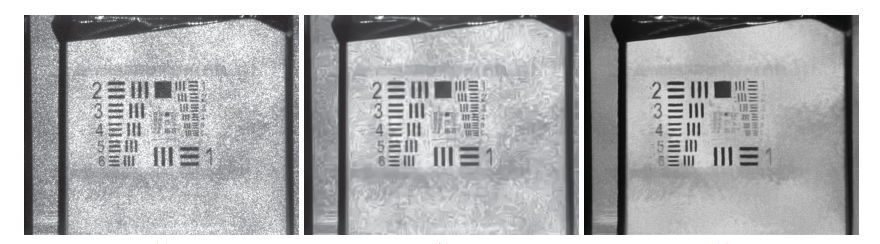
Figure 1: Example image restoration of real world images by Dong et al. ^[5]

In the literature, various image denoising methods already exist. Some of them, explicitly estimate edge structures and try to preserve them in the denoised images. For example, Mukherjee and Qiu^[10] proposed a denoising procedure which uses local clustering of pixels based on their observed intensity values. In this method they cluster the neighborhood of pixel into two clusters using the intensity values and use the pixels corresponding to the cluster of the given pixel for smoothing procedure. An advantage of this method is that these does not require explicit edge detection and complex edge structures can be preserved using this method. Qiu and Mukherjee^[11] also introduced an image denoising method that first detects edges, estimates them locally using two intersecting half-lines, and then smooths the observed image intensities within a neighborhood where pixels are located on one side of the estimated edge curve.There are also jumpe-regression analysis based methods (eg Gijbels et al. ^[8]), but these have the drawback of blurring complicated edge structures.
Another major type of denoising methods obtain edge information to use in the smoothing process without estimating the underlying edge structure directly. Bilateral filtering methods (e.g Gavaskar and Chaudhury^[7]) assign weights base on edge information in there smoothing process. Similarly, Anistropic diffusion methods (e.g. Bai et al.^[1])control the strength and direction of smoothing based on the underlying edge information. Takeda et al.^[13] proposed an adaptive smoothing method based on steering kernel regression, in which they choose the shape and size of the neighborhood depending on the local edge structure. For pixels near edge structures the neighborhood chosen by the method is elongated along the edge so that the neighborhood contain minimal number of pixels form the edges and the other side of edge. But, in cases where they contain pixels from both side of edges they result blurring the image.
Apart from these two approaches, there are various other denoising methods in the literature. The non-local means algorithms (Buades et al.^[2],[3],Lie et al.^[9],Froment^[6]) calculates similarity scores between pixels and use them as weights to provide noise free estimates. Wavelet transformation (e.g Chang et al. ^[4]) methods rely on predefined basis functions, with the denoised image being a linear combination of these functions. The performance of these methods greatly depends on the selection of basis functions.
In this paper, we propose a novel denoising technique which integrates explicit edge detection and adaptive smoothing to preserve edge structure while efficiently choosing larger neighborhoods to make the denoising performance better. This method will utilize explicit edge detection to determine neighborhood shapes and sizes specifically for pixels located farther from edge structures. For pixels nearer to edges, we can employ clustering methods to achieve enhanced performance, particularly around intricate edge configurations. In Section 2 we will be discussing the methodology in detail and in Section 3 we will present some numerical studies and comparisons with other competing methods.

2 Proposed Methodology

2.1 Identifying the edge pixels

We first identify the edge pixels in a given image. The intensities at a given pixel is given by :

$$z_{ij}=f(x_{i},y_{i})+\epsilon_{ij}\hskip 7.22743ptfor\hskip 7.22743pti,j=1,2,\dots,n$$

where $\{(x_{i},y_{j})=(i/n,j/n),i,j=1,2,\dots,n\}$ are equally spaced design points or pixels. $\{\epsilon_{i,j}\}$ are iid random variables with mean $\mu$ and variance $\sigma^{2}$. $f(x,y)$ is continuous over $[0,1]\times[0,1]$ except on some curves which is called the jump location curve or JLC. A point (i,j) is called a singular point if it satisfies at least one of the following conditions:

• There exists some constant $\zeta_{0}>0$ such that for any $0<\zeta<\zeta_{0}$ the neighborhood of $(i,j)$ of diameter $\zeta$ is divided into more than two connected region by the JLCs.

• There exists no such constant $\rho_{0}>0$ such that there exist two orthogonal lines crossing at $(i,j)$and two vertical quadrants formed by these two line belong to two different regions separated by a JLC in a neghborhood of $(i,j)$ with diameter $\rho_{0}$.

Consider

$$N(x_{i},y_{i})=\{(x_{i+s},y_{j+t}),s,t=-l,-l+1,\dots,0,\dots,l--1,l\}$$

and we are trying to fit a least square plane in this neighborhood:

$$\hat{z}_{ij}(x,y)=\hat{\beta}_{0}^{(i,j)}+\hat{\beta}_{1}^{(i,j)}(x-x_{i})+\hat{\beta}_{2}^{(i,j)}(y-y_{j}),\hskip 7.22743pt(x,y)\in N(x_{i},y_{j})$$

We can estimate the gradients of intensity using $\beta_{1},\beta_{2}$. And if $P1\text{, }P2$ are neighboring pixels of $(i,j)$ along the gradient, then consider :

$$\delta_{ij}=min(||\vec{v}_{ij}-\vec{v}_{P1}||,||\vec{v}_{ij}-\vec{v}_{P2}||)\hskip 7.22743pt\text{where }\vec{v}_{ij}=(\hat{\beta}_{1}^{(i,j)},\hat{\beta}_{2}^{(i,j)}).$$

And Qiu and Yandoll^[12] has proven the following theorems showing that under some assumptions, $\delta_{ij}>\hat{\sigma}\sqrt{\frac{\chi^{2}_{2,\alpha_{n}}}{kS_{x}^{@}}}$ can be used as an indicator of an edge pixel. Here $k$ is the window width and $\chi^{2}_{2,\alpha_{n}}$ is the $(1-\alpha_{n})^{th}$ quantile of $\chi^{2}_{2}$ distribution. We are using this method to detect edge pixels in an image.

Lemma 2.1.

Assume that $f(x,y)$ has continuous first order partial derivatives over $(0,1)\times(0,1)$ except on the JLCs and it has the first order right and left partial derivatives at the JLCs.And also $\lim_{n\rightarrow\infty}k=\infty$ and $\lim_{n\rightarrow\infty}k/n=0$ where $k$ is the window width. If there is no jump in $N\left(x_{i},y_{j}\right)$, then

$$\hat{\beta}_{1}^{(i,j)}=f_{x}^{\prime}\left(x_{i},y_{j}\right)+O\left(\frac{n\sqrt{\log\log k}}{k^{2}}\right)\text{, a.s. }$$

and

$$\hat{\beta}_{2}^{(i,j)}=f_{y}^{\prime}\left(x_{i},y_{j}\right)+O\left(\frac{n\sqrt{\log\log k}}{k^{2}}\right)\text{, a.s. }$$

If $\left(x_{i},y_{j}\right)$ is on a JLC and it is not a singular point, then

$$\hat{\beta}_{1}^{(i,j)}=f_{x}^{\prime}\left(\tilde{x}_{i},\tilde{y}_{j}\right)+h_{1}^{(i,j)}C(i,j)+\gamma_{1}C_{x}(i,j)+O\left(\frac{n\sqrt{\log\log k}}{k^{2}}\right)\text{, a.s. }$$

and

$$\hat{\beta}_{2}^{(i,j)}=f_{y}^{\prime}\left(\tilde{x}_{i},\tilde{y}_{j}\right)+h_{2}^{(i,j)}C(i,j)+\gamma_{2}C_{y}(i,j)+O\left(\frac{n\sqrt{\log\log k}}{k^{2}}\right)\text{, a.s. }$$

where $\left(\tilde{x}_{i},\tilde{y}_{j}\right)$ is some point around $\left(x_{i},y_{j}\right)$ on the same side of the JLC as $\left(x_{i},y_{j}\right)$ and the distance between $\left(\tilde{x}_{i},\tilde{y}_{j}\right)$ and $\left(x_{i},y_{j}\right)$ tends to zero; $C(i,j),C_{x}(i,j)$, and $C_{y}(i,j)$ are the jump magnitudes of $f(x,y)$ and its first order $x$ and y partial derivatives; $h_{1}^{(i,j)}$ and $h_{2}^{(i,j)}$ are two constants satisfying

$$\sqrt{\left(h_{1}^{(i,j)}\right)^{2}+\left(h_{2}^{(i,j)}\right)^{2}}=O(n/k)$$

$\gamma_{1}$ and $\gamma_{2}$ are two constants between $-1$ and 1 .

Lemma 2.2.

Besides the conditions stated above, if there are only finite number of singular points on JLCs and $\alpha_{n}$ is chosen such that

1. $\lim_{n\rightarrow\infty}\alpha_{n}=$ $0;$

2. $\lim_{n\rightarrow\infty}\log\left(\alpha_{n}\right)/\log(\log(k))=-\infty$;

3. and $\lim_{n\rightarrow\infty}\log\left(\alpha_{n}\right)/k^{2}=0$,

then the detected jumps are a.s. consistent in the Hausdorff distance and the convergence rate is $O\left(n^{-1}\log(n)\right)$.

From the above results we can say that if we choose $\alpha_{n}=O(1/log(log(n))$ and $k=O(n^{\beta})$ where $\beta<1$, all the above conditions are satisfied for edge detection.

2.2 Smoothing

Next for each given pixel, we try to find out and ellipse around the given pixels such that no edge pixels are inside it. To do this:

1. We first find out the nearest edge pixel to $P$, where $P$ is point where we want to fit the smoothed value. Call this point $P_{1}$,

2. Next we consider the point $M$, which is the reflection of the point $P_{1}$ with respect to the given point. Then we find the nearest edge pixel in the strip perpendicular to the line joining $M$ and $P_{1}$, say $P_{2}$.

3. now the consider the ellipse $E$, which is centered at $P$ and chose such that $d(P_{1},E)>\gamma$ and $d(P_{2},E)>\gamma$. Here $\gamma$ is a tuning parameter.

We then use a suitable kernel which is non-negative inside $E$ and zero outside it, and find out the smoothed value at $P$ using kernel regression. In kernel regression we take the measured pixel intensities are given by :

$$z_{\tilde{x}}=f(\tilde{x})+\epsilon_{\tilde{x}}$$

Where $f$ is an unknown function. Here we assume $f$ to be smooth up to $N^{th}$ order, so if $\tilde{x}_{i}$ is near $\tilde{x}$ the we can use Taylor expansion to get:

$$z(\tilde{x}_{i}) \approx z(\tilde{x})+(\nabla z(\tilde{x}))^{T}(\tilde{x}_{i}-\tilde{x})+\frac{1}{2}(\tilde{x}_{i}-\tilde{x})^{T}\mathcal{H}z(x)(\tilde{x}_{i}-\tilde{x})+\dots$$

$$=\beta_{0}+\beta_{1}^{T}(\tilde{x}_{i}-\tilde{x})+\beta_{2}^{T}vech{(\tilde{x}_{i}-\tilde{x})(\tilde{x}_{i}-\tilde{x})^{T}}+...$$

where $\beta_{0}=z(\tilde{x})$, $\beta_{1}=\nabla z(\tilde{x})$, $\beta_{2}=\frac{1}{2}[\frac{\partial^{2}z(\tilde{x}}{\partial\tilde{x}_{1}^{2}},2\frac{\partial^{2}z(\tilde{x}}{\partial\tilde{x}_{1}\partial\tilde{x}_{2}},\frac{\partial^{2}z(\tilde{x}}{\partial\tilde{x}_{2}^{2}}]$ and $vech(\begin{pmatrix}a&b\\ b&d\end{pmatrix}=(a,b,d)$
So we can formulate this as a regression problem and estimate $\beta_{0}$,$\beta_{1}$, $\dots$ by minimizing :

$$\sum_{i=1}^{P}\bigg{[}z(\tilde{x}_{i})-\beta_{0}-\beta_{1}^{T}(\tilde{x}_{i}-\tilde{x})-\beta_{2}^{T}vech{(\tilde{x}_{i}-\tilde{x})(\tilde{x}_{i}-\tilde{x})^{T}}+...\bigg{]}^{2}K(\tilde{x}_{i}-\tilde{x})$$

with $K$ as a kernel of our choice. We do this only in points where the distance between $P$ and $P_{1}$ is large enough.

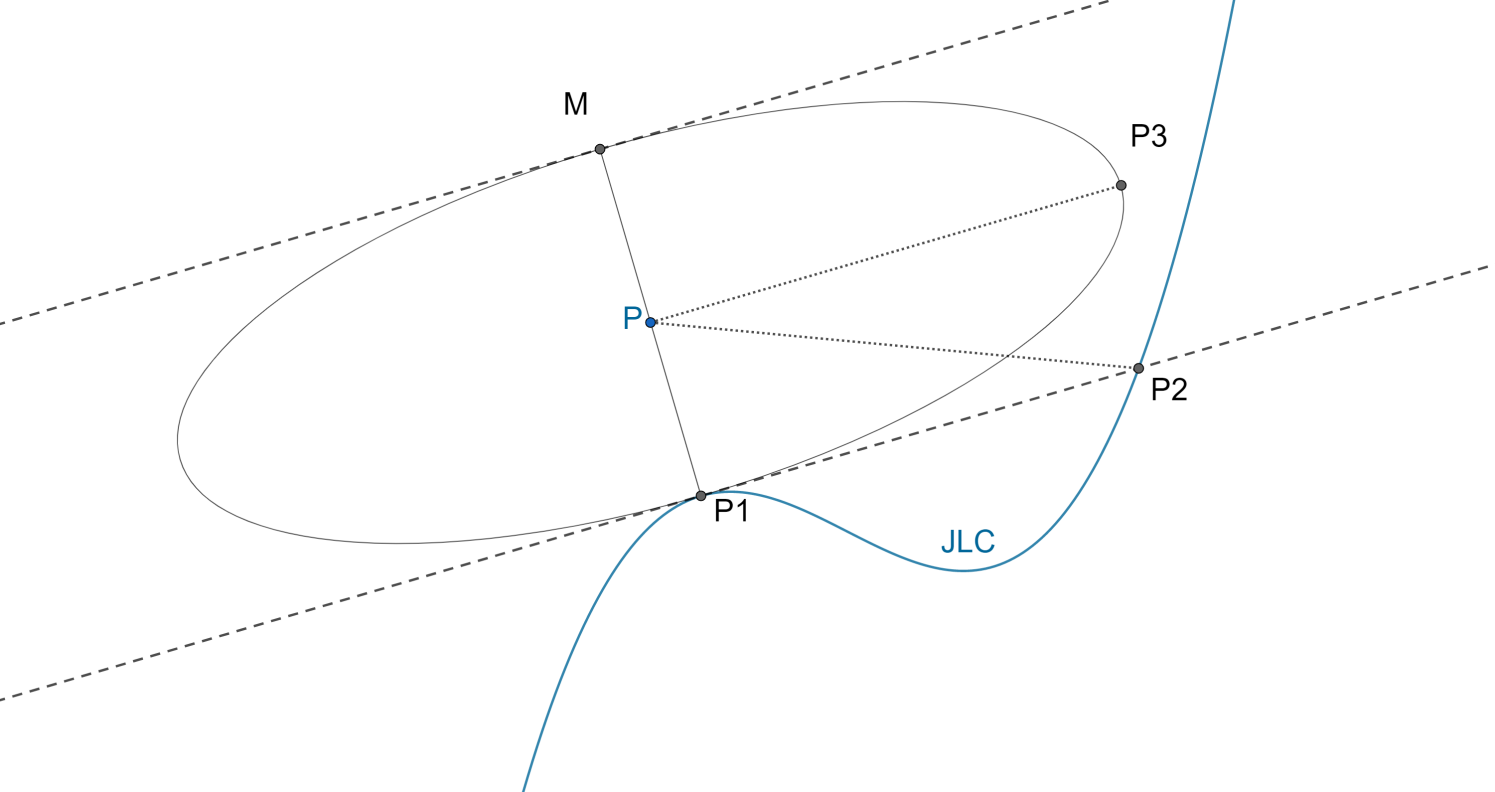
Figure 2: Figure showing how neighborhood for regression is selected

For pixels which are closer to the detected edge pixels,i.e within $\gamma$ distance of an edge pixel, we are using the clustering method proposed by Mukherjee and Qiu ^[10]. Consider a neighborhood $O(x,y,h_{n})$ around one such point $(x,y)$. We can choose a threshold $s$, so that the pixels with intensity value $z_{ij}\leq s$ are i one cluster. Then we are choosing s such that it minimizes $T(x,y,h_{n},s)$, the ratio of between-group and within-group variability of the intensity values.

$$T(x,y,h_{n},s)=\frac{|O_{1}(x,y,h_{n},s)|(\bar{z_{1}}-\bar{z})^{2}+|O_{2}(x,y,h_{n},s)|(\bar{z_{2}}-\bar{z})^{2}}{\sum\limits_{(x_{i},y_{j})\in O_{1}(x,y,h_{n},s)}(z_{ij}-\bar{z_{1}})^{2}+\sum\limits_{(x_{i},y_{j})\in O_{2}(x,y,h_{n},s)}(z_{ij}-\bar{z_{2}})^{2}}$$

Where $O_{1}(x,y,h_{n},s)$ and $O_{2}(x,y,h_{n},s)$ are the two clusters created using threshold $s$. And $\bar{z_{1}}$ and $\bar{z_{2}}$ are the average of intensity values in the respective clusters. We can choose the optimal value of $s$ using:

$$S_{0}=\text{arg}\max T(x,y,h_{n},s)$$

After dividing the neighborhood $O(x,y,h_{n})$ into to clusters, we can estimate the true image intensity at $(x,y)$ using the weighted average of intensity values of the pixels in the cluster corresponding to $(x,y)$ . Here we are using a similarity measure between pixels as weights, which is given by :

$$\tilde{W_{ij}}=exp\Bigg{(}-\frac{||\tilde{O}(x_{i},y_{j})-\tilde{O}(x,y)||^{2}_{2}}{2\hat{\sigma}^{2}|\tilde{O}(x_{i},y_{j})|B_{n}})\Bigg{)}$$

where, $\tilde{O}(x,y)$ is a neighborhood around $(x,y)$ of radius $\tilde{h_{n}}$, $\hat{\sigma}$ is the estimated standard deviation of errors. and $B_{n}$ is a tuning parameter. We are using $L_{2}$ distance between the observed intensity values as the distance here.
Next, consider the following notations.

$$\Omega_{\epsilon} =[\epsilon,1-\epsilon]\times[\epsilon,1-\epsilon],$$

$$J_{\epsilon} =\left\{(x,y):(x,y)\in\Omega,d_{E}\left((x,y),\left(x^{*},y^{*}\right)\right)\leq\epsilon\text{ for some }\left(x^{*},y^{*}\right)\in D\right\},$$

$$S_{\epsilon} =\left\{(x,y):(x,y)\in\Omega,d_{E}\left((x,y),\left(x^{*},y^{*}\right)\right)\leq\epsilon\text{ for a singular point }\left(x^{*},y^{*}\right)\in D\right\},$$

$$\Omega_{\bar{J},\epsilon} =\Omega_{\epsilon}\backslash J_{\epsilon},$$

$$\Omega_{\bar{S},\epsilon} =\Omega_{\epsilon}\backslash S_{\epsilon},$$

Mukherjee and Qiu ^[10] have shown the following results to prove the consistency of the method explained above.

Lemma 2.3.

Assume that $f$ has continuous first-order derivatives over $(0,1)\times(0,1)$ except on the JLCs, its first order derivatives have one-sided limits at non-singular points of the JLCs, $\left\{\varepsilon_{ij}\right\}$ are i.i.d. and have the common distribution $N\left(0,\sigma^{2}\right)$, where $0<\sigma<\infty$, $h_{n}=o(1),1/nh_{n}=o(1),u_{n}=\kappa+\delta$, where $\kappa=\left(\frac{\phi^{2}(0)}{\Phi(0)(1-\Phi(0))}\right)/\left[1-\left(\frac{\phi^{2}(0)}{\Phi(0)(1-\Phi(0))}\right)\right],\delta$ is any positive number, and $\phi$ and $\Phi$ are the probability density function and the cumulative distribution function of the $N(0,1)$ distribution, respectively. Then, we have

(i) if $(x,y)\in\Omega_{\bar{J},\epsilon}$, then $T\left(x,y;h_{n},S_{0}\right)\leq u_{n}$, a.s. (ii) on the other hand, if a non-singular point $(x,y)\in J_{h_{n}}$, and the minimum jump size of the JLC within $O\left(x,y;h_{n}\right)$ is larger than $4\kappa\sigma^{2}$, then $T\left(x,y;h_{n},S_{0}\right)>u_{n}$, a.s.

Lemma 2.4.

Under the assumptions in Lemma 2.3, if we further assume that $B_{n}=$ $O\left(h_{n}^{1/2}\right)$, then for any non-singular $(x,y)\in\Omega_{\bar{S},\epsilon}$, we have $\widehat{f}(x,y)=f(x,y)+O\left(h_{n}^{1/2}\right)$, a.s.

Now suppose we are using $\bar{h_{n}}$ window width and $\alpha_{n}$ confidence level for edge detection and $h_{n}$ window width and $\gamma_{n}$ as tuning parameter for the smoothing process. Then the following holds:

Theorem 2.5.

Assume that f has continuous first-order derivatives over $(0,1)\times(0,1)$ except on KLCs and the first order right and left derivative exists at the JLCs, $\epsilon_{ij}$ are iid and have distribution $N(0,\sigma^{2})$ with $0<\sigma^{2}<\infty$. And we have $\bar{h_{n}}=O(n^{\beta}))$ with $\beta<1$, $\alpha_{n}=O(1/\log\log n)$, $h_{n}=o(1)$, $1/nh_{n}=o(1)$ and constant $\gamma<1$. Then for any non-singular (x,y) with the property $d((x,y),(x^{*},y^{*}))>\epsilon\forall$ singular points $(x^{*},y^{*})$ we have $\hat{f}(x,y)=f(x,y)+o(\sqrt{h_{n}})$. where $\hat{f}(x,y)$ are the estimates produces by the proposed method.

Proof.

Let $J$ denote the points on JLCs and $\hat{J_{n}}$ denote the detected edge pixels. Suppose we are given the point $(\tilde{x},\tilde{y})$.

Suppose the point is not on $J$. Then as $\mathcal{H}(J,\hat{J}_{n})\rightarrow 0$, for large enough n it is not in $\hat{J}_{n}$ wp 1.So wlog we assume it is not on $\hat{J}_{n}$ . Suppose the nearest point on $\hat{J}_{n}$ is $(x,y)$.
There exists $N$ st for all $n>N$ we have $\mathcal{H}(J,\hat{J_{n}})<\gamma$. So we can say $\forall n>N$ there is a circle around $(x,y)$ of radius $d((x,y),(\tilde{x},\tilde{y}))-\gamma$ which does not touch $\hat{J_{n}}$.

Now, for choosing the 2nd closest point in our algorithm( point $P2$ in figure 2), we are doing the same as above while restricting the image in that strip. So we can take $\hat{\Omega}=\Omega\cap S$ and $\hat{J}^{{}^{\prime}}_{n}=\hat{J}_{n}\cap S$, where $S$ is the strip chosen using the first step. So from the fact that the ellipse we define is completely inside the strip and using the same argument as choosing the first point we can say that the ellipse we are choosing has no point which are on JLC. So. $f(x)$ hase continuous first order derivatives inside the ellipse E. So the Taylor series converges, Hence $\hat{f}(x)\rightarrow f(x)$.

Now if $(\tilde{x},\tilde{y})$ is on J. Then as $\mathcal{H}(J,\hat{J}_{n})\rightarrow 0$, we can say, $d((\tilde{x},\tilde{y}),\hat{J}_{n})<\gamma$ for large enough n. So, for large enough n we will be using the method proposed by Mukherjee and Qiu ^[10]. So, by Result (2.4) we get, $\hat{f}(x)\rightarrow f(x)$.

∎

3 Comparison with other methods

In the following figures we demonstrate how our algorithm works on different types of images.We have compared it with number of methods including the steering kernel algorithm suggested by Takeda et al^[13] and the clustering method proposed by Mukherjee and Qiu^[10].In the steering kernel algorithm the neighborhood around each pixel is chosen in such a way so that the neighbor hood becomes elongated parallel to the edge if he chose pixel is near an edge structure. Since this method employs a similar idea as our proposed method we have chosen it to include in our comparison.
In the following figures we have added Gaussian noise of 5,10 and 20 standard deviation on each row, respectively.

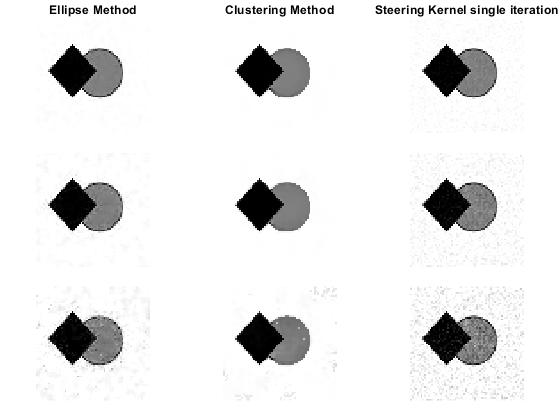
Figure 3: Comparison with competing methods.

RMSE
Ellipse Method	2.61	4.67	9.81
Clustering Method	8	8.11	9.9
Steering Kernel	3.01	5.22	11.18

Figure 4: Comparison with competing methods.

RMSE
Ellipse Method	4.41	6.43	10.27
Clustering Method	4.45	6.45	10.53
Steering Kernel	3.27	5.95	14.45

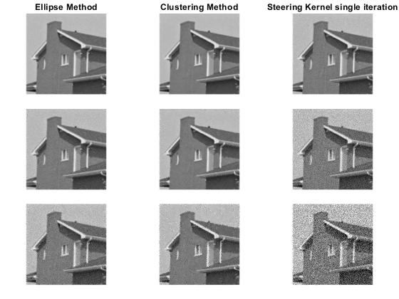
Figure 5: Comparison with competing methods.

RMSE
Ellipse Method	2.51	4.37	7.99
Clustering Method	2.52	4.6	8.69
Steering Kernel	1.97	4.85	13.45

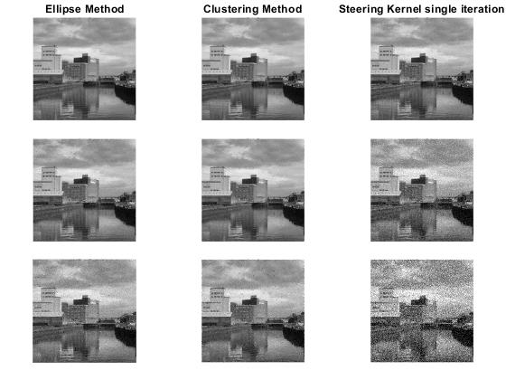
Figure 6: Comparison with competing methods.

RMSE
Ellipse Method	2.8	4.77	8.2
Clustering Method	2.89	4.87	8.45
Steering Kernel	2.12	4.93	13.46

From Figures 3 ,4 5 and 6, we can see that our method performs better when the edges in the given images are defined clearly. So it performs better for the test image we used. But where the edges are not obvious or there are multiple edges with similar direction in a small neighborhood, performance of our algorithm is affected. We can see it clearly when we apply the algorithm on real images as these cases frequently occur there. For real images, the other two methods perform better when noise is low. However, our algorithm gives better results at higher noise levels, as errors due to poorly defined edges become minimal compared to noise. Here, we used only one iteration for the steering kernel algorithm.

4 Conclusion

In this paper, we proposed a denoising procedure which detects edge structures and then proceed to denoising using adaptive kernel regression or local clustering depending on the underlying edge structure. And we have also shown that it show increase in performance when compared to similar methods already in literature. We have also show that under some constraints the denoised image converges to the true image for large enough images. However, there are improvements to be made. The edge detection method we used uses the same radius of neighborhood throughput the whole image, we can improve this by choosing differently sized neighborhood for different pixels depending on local standard deviation to better the edge detection performance which further improves the denoising performance. Computation time for our algorithm can also be improved. We can also try to generalize this method for 3D images. We plan to address all these issues in our future research.

References

- [1] Jian Bai and Xiang-Chu Feng “Fractional-order anisotropic diffusion for image denoising” In IEEE transactions on image processing 16.10 IEEE, 2007, pp. 2492–2502
- [2] Antoni Buades, Bartomeu Coll and J-M Morel “A non-local algorithm for image denoising” In 2005 IEEE computer society conference on computer vision and pattern recognition (CVPR’05) 2, 2005, pp. 60–65 Ieee
- [3] Antoni Buades, Bartomeu Coll and Jean-Michel Morel “Image denoising methods. A new nonlocal principle” In SIAM review 52.1 SIAM, 2010, pp. 113–147
- [4] S Grace Chang, Bin Yu and Martin Vetterli “Spatially adaptive wavelet thresholding with context modeling for image denoising” In IEEE Transactions on image Processing 9.9 IEEE, 2000, pp. 1522–1531
- [5] Weisheng Dong, Guangming Shi and Xin Li “Nonlocal Image Restoration With Bilateral Variance Estimation: A Low-Rank Approach” In IEEE Transactions on Image Processing 22.2, 2013, pp. 700–711 DOI: 10.1109/TIP.2012.2221729
- [6] Jacques Froment “Parameter-free fast pixelwise non-local means denoising” In Image Processing On Line 4, 2014, pp. 300–326
- [7] Ruturaj G. Gavaskar and Kunal N. Chaudhury “Fast Adaptive Bilateral Filtering” In IEEE Transactions on Image Processing 28.2, 2019, pp. 779–790 DOI: 10.1109/TIP.2018.2871597
- [8] Irene Gijbels, Alexandre Lambert and Peihua Qiu “Jump-preserving regression and smoothing using local linear fitting: a compromise” In Annals of the Institute of Statistical Mathematics 59 Springer, 2007, pp. 235–272
- [9] Yan-Li Liu et al. “A robust and fast non-local means algorithm for image denoising” In Journal of computer science and technology 23.2 Springer, 2008, pp. 270–279
- [10] Partha Sarathi Mukherjee and Peihua Qiu “Image denoising by a local clustering framework” In Journal of Computational and Graphical Statistics 24.1 Taylor & Francis, 2015, pp. 254–273
- [11] Peihua Qiu and Partha Sarathi Mukherjee “Edge structure preserving image denoising” In Signal Processing 90.10 Elsevier, 2010, pp. 2851–2862
- [12] Peihua Qiu and Brian Yandell “Jump detection in regression surfaces” In Journal of Computational and Graphical Statistics 6.3 Taylor & Francis, 1997, pp. 332–354
- [13] Hiroyuki Takeda, Sina Farsiu and Peyman Milanfar “Kernel regression for image processing and reconstruction” In IEEE Transactions on image processing 16.2 IEEE, 2007, pp. 349–366