Accelerated Primal-Dual Proximal Gradient Splitting Methods for Convex-Concave Saddle-Point Problems

Abstract

In this paper, based a novel primal-dual dynamical model with adaptive scaling parameters and Bregman divergences, we propose new accelerated primal-dual proximal gradient splitting methods for solving bilinear saddle-point problems with optimal nonergodic convergence rates. For the first, using the spectral analysis, we show that a naive extension of Nesterov acceleration to a quadratic game is unstable. Motivated by this, we present an accelerated primal-dual hybrid gradient (APDHG) flow which combines acceleration with careful velocity correction. To work with non-Euclidean distances, we also equip our APDHG model with general Bregman divergences and prove the exponential decay of a Lyapunov function. Then, new primal-dual splitting methods are developed based on proper semi-implicit Euler schemes of the continuous model, and the theoretical convergence rates are nonergodic and optimal with respect to the matrix norms,  Lipschitz constants and convexity parameters. Thanks to the primal and dual scaling parameters, both the algorithm designing and convergence analysis cover automatically the convex and (partially) strongly convex objectives. Moreover, the use of Bregman divergences not only unifies the standard Euclidean distances and general cases in an elegant way, but also makes our methods more flexible and adaptive to problem-dependent metrics.

1 Introduction

Consider the convex-concave saddle-point problem

$$\min_{x\in\,{\mathbb{R}}^{n}}\max_{y\in\,{\mathbb{R}}^{m}}\,\mathcal{L}(x,y)=f(x)+\left\langle{Ax,y}\right\rangle-g(y),$$ (1)

where $f:\,{\mathbb{R}}^{n}\to\,{\mathbb{R}}\cup\{+\infty\}$ and $g:\,{\mathbb{R}}^{m}\to\,{\mathbb{R}}\{\infty\}$ are properly closed convex functions and $A\in\,{\mathbb{R}}^{m\times n}$ is a linear operator. This model problem arises from many practical applications such as image processing [13], numerical partial differential equations [8], machine learning [40], and optimal transport [7]. We are mainly interested in first-order methods that involve the (proximal) gradient information of the objective $f/g$; see the proximal algorithm class [81, Definition 2.1] for instance.

The saddle-point problem 1 is closely related to many convex optimization problems. Obviously, it contains the unconstrained composite convex minimization

$$\min_{x\in\,{\mathbb{R}}^{n}}\,P(x):=f(x)+g^{*}(Ax),$$ (2)

for which the dual problem reads equivalently as

$$\min_{y\in\,{\mathbb{R}}^{m}}\,D(y):=g(y)+f^{*}(-A^{\top}y).$$ (3)

When $g^{*}$ (or $f^{*}$) is the indicator function of a simple convex set $\mathcal{K}$, the primal problem 2 (or the dual problem 3) also corresponds to the standard affinely constrained problem

$$\min_{x\in\,{\mathbb{R}}^{n}}\,f(x)\quad{{\rm s.t.}\,}\,Ax\in\mathcal{K}.$$ (4)

Besides, one can replace $Ax$ (or $A^{\top}y$) with an auxiliary variable, and the unconstrained minimization 2 (or 3) becomes a special case of the two-block separable problem

$$\min_{x_{1}\in\,{\mathbb{R}}^{n},\,x_{2}\in\,{\mathbb{R}}^{m}}\,f_{1}(x_{1})+f_{2}(x_{2})\quad{{\rm s.t.}\,}\,A_{1}x_{1}+A_{2}x_{2}=b,$$ (5)

which can be recast into the saddle-point problem 1 by using the Lagrange function.

1.1 Literature review

As mentioned before, the minimax formulation 1 is usually equivalent to the unconstrained composite problem 2. In this regard, classical first-order methods include proximal gradient [65], forward-backward splitting [42], Douglas–Rachford splitting (DRS) [23], and accelerated gradient methods [6, 16, 45, 51, 61]. As for linearly constrained problems 4 and 5, prevailing algorithms are quadratic penalty methods [41, 71], Bregman iteration [11], augmented Lagrangian methods (ALM) [5, 46, 47, 49] and alternating direction methods of multipliers (ADMM) [25, 52, 63, 68, 79, 82].

1.1.1 Primal-dual splitting

In the following, we mainly review existing primal-dual splitting methods that applied directly to the saddle-point problem 1. Zhu and Chan [84] proposed the primal-dual hybrid gradient (PDHG) method:

$$\left\{\begin{aligned} x_{k+1}={}&\mathop{{\mathop{{\rm argmin}}\,}}\limits_{x\in\,{\mathbb{R}}^{n}}\mathcal{L}(x,y_{k})+\frac{1}{2\tau}\left\lVert{x-x_{k}}\right\rVert^{2},\quad\tau>0,\\ y_{k+1}={}&\mathop{{\mathop{{\rm argmax}}\,}}\limits_{y\in\,{\mathbb{R}}^{m}}\mathcal{L}(x_{k+1},y)-\frac{1}{2\sigma}\left\lVert{y-y_{k}}\right\rVert^{2},\quad\sigma>0,\end{aligned}\right.$$ (6)

which actually corresponds to the well-known Arrow–Hurwicz method [1]. However, even for extremely small steplengths, PDHG is not necessarily convergent unless one of the objectives is strongly convex; see the counterexamples in [27]. Later on, Chambolle and Pock [12] presented a generalized version (CP for short)

$$\left\{\begin{aligned} x_{k+1}={}&\mathop{{\mathop{{\rm argmin}}\,}}\limits_{x\in\,{\mathbb{R}}^{n}}\mathcal{L}(x,y_{k})+\frac{1}{2\tau}\left\lVert{x-x_{k}}\right\rVert^{2},\\ \bar{x}_{k+1}={}&x_{k+1}+\theta(x_{k+1}-x_{k}),\\ y_{k+1}={}&\mathop{{\mathop{{\rm argmax}}\,}}\limits_{y\in\,{\mathbb{R}}^{m}}\mathcal{L}(\bar{x}_{k+1},y)-\frac{1}{2\sigma}\left\lVert{y-y_{k}}\right\rVert^{2},\end{aligned}\right.$$ (7)

where $\theta\in(0,1]$ denotes the relaxation parameter. When $\theta=0$, CP amounts to PDHG, and it is also closely related to many existing methods such as the extra-gradient method [38], DRS [62], and the preconditioned ADMM [67, 69]. In [28], He and Yuan discovered that CP can be reformulated as a tight proximal point algorithm (PPA), and the relaxation parameter $\theta\in(0,1]$ can be further extended to $\theta\in[-1,1)$, with proper correction steps (see [28, Algorithms 1 and 2]). However, these extra steps involve additional matrix-vector multiplications. As discussed in [76, Remark 2.3], it is possible to extend the PPA framework of CP to the non-Euclidean setting with general Bregman distances. This is in line with the spirit of the mirror-descent method by Nemirovski [55]; see [14, 19, 20, 73] and the references therein. For more extensions of CP, with preconditioning, extrapolation/correction and inexact variants, we refer to [26, 36, 43, 85].

Assumption	${\mu_{\!f}}={\mu_{g}}=0$	${\mu_{\!f}}+{\mu_{g}}>0$	${\mu_{\!f}}{\mu_{g}}>0$
Rate	$\mathcal{O}\left(\frac{1}{k}\right)$	$\mathcal{O}\left(\frac{1}{k^{2}}\right)$	$\mathcal{O}\left(\exp\left(-\frac{k}{\sqrt{\kappa_{P}}}\right)\right)$
Refs.	[4, 12, 14, 21, 36]	[14, 36, 53]	[14, 36]
	[53, 72, 74, 78]	[72, 74, 78]	[66, 72]
	[70, 73, 75]*	[12, 33, 75]*	[12, 75]*
	This work*

Table 1: Summary of convergence rates of existing primal-dual methods for solving 1. Nonergodic results are marked with “*”. Here, $\mu_{f},\,\mu_{g}\geq 0$ are respectively the strong convexity constants of $f$ and $g$, and $\kappa_{P}:=\left\lVert{A}\right\rVert^{2}/({\mu_{\!f}}{\mu_{g}})$ stands for the condition number of the primal problem 2.

According to [12, 14], CP converges with an ergodic sublinear rate $\mathcal{O}(1/k)$ for generic convex-concave problems, and fast (ergodic) sublinear/linear rates can also be achieved for (partially) strongly convex case ${\mu_{\!f}}+{\mu_{g}}>0$; see Table 1 for a summary of related works on convergence rates. However, from the literature, it is rare to see nonergodic results, which, as mentioned by Chambolle and Pock in [14, Section 8], converge very often much faster than the sense of ergodic. We mention that linear convergence can still be obtained even for non-strongly convex problems [24, 39, 44] and nonergodic convergence with respect to fixed-point type residual can be found in [26, 37].

Recently, based on the PPA structure of CP and the testing approach [76], Valkonen [75] proposed the inertial corrected primal-dual proximal splitting (IC-PDPS), which achieves the optimal sublinear/linear nonergodic rates (cf.Table 1). In [48], we provided a continuous-time perspective on IC-PDPS, which can be viewed as an implicit-explicit time discretization of a novel primal-dual dynamics.

When the primal (dual) objective $f$ ($g$) in 1 possesses the composite structure $f=f_{1}+f_{2}$ ($g=g_{1}+g_{2}$), where the smooth part $f_{1}$ ($g_{1}$) has Lipschitz continuous gradient, some existing primal-dual splitting methods [17, 19, 34, 39, 78] possess optimal mixed-type complexity bounds; see Table 2. Compared with these works, our methods cover both convex ($\mu_{f}=\mu_{g}=0$) case and partially convex case ($\mu_{f}+\mu_{g}>0$). Especially, it is rare to see the mixed-type result for $\mu_{f}>0$ and $\mu_{g}=0$.

	${\mu_{\!f}}=0$		${\mu_{\!f}}>0$
${\mu_{g}}=0$	$\mathcal{O}\left(\frac{\left\lVert{A}\right\rVert}{\epsilon}+\sqrt{\frac{{L_{\!f}}}{\epsilon}}\right)$	[19, 59, 60]	$\mathcal{O}\left(\frac{\left\lVert{A}\right\rVert}{\sqrt{{\mu_{\!f}}\epsilon}}+\sqrt{\kappa_{\!f_{1}}}\left\lvert{\ln\epsilon}\right\rvert\right)$
		[34, 78]⋆
		This work	This work
${\mu_{g}}>0$	$\mathcal{O}\left(\frac{\left\lVert{A}\right\rVert}{\sqrt{{\mu_{g}}\epsilon}}+\sqrt{\frac{{L_{\!f}}}{\epsilon}}\right)$	[59] [78]⋆	$\mathcal{O}\left(\sqrt{\kappa_{P}+\kappa_{\!f_{1}}}\left\lvert{\ln\epsilon}\right\rvert\right)$
		This work	[17, 39]  This work

Table 2: Summary of existing mixed-type complexity bounds for solving 1 under the composite structure $f=f_{1}+f_{2}$, where $f_{1}$ is ${\mu_{\!f}}$-convex with ${L_{\!f}}$-Lipschitz continuous gradient. Ergodic results are marked with “$\star$”. Again $\kappa_{P}=\left\lVert{A}\right\rVert^{2}/({\mu_{\!f}}{\mu_{g}})$ is the condition number of 2 and $\kappa_{\!f_{1}}={\mu_{\!f}}/{L_{\!f}}$ is the condition number of $f_{1}$.

1.1.2 Smoothing

Except primal-dual splitting methods based on the PPA framework mentioned above, let us also review other works with smoothing technique. For nonsmooth composite convex optimization problems with the minimax structure (like 1), Nesterov [60] combined his accelerated gradient [57] with smoothing and improved the iteration complexity of subgradient-type methods from $\mathcal{O}(1/\epsilon^{2})$ [56] to $\mathcal{O}(1/\epsilon)$. Afterwards, there are primal-dual methods based on the excessive gap technique (double smoothing approach) [22, 59] and homotopy strategy (adaptively changing smoothing parameters) [70].

In [73], Tran-Dinh et al. proposed two accelerated smoothed gap reduction (ASGARD) algorithms and established the optimal sublinear rate $\mathcal{O}(1/k)$ for the primal objective residual. The unified variant of ASGARD in [72] and two primal-dual algorithms in [74] achieve optimal sublinear/linear rates for the primal-dual gap, the primal objective residual, and the dual objective residual. However, it should be noticed that (i) both [73, Algorithm 2] and [74, Algorithm 2] involve three proximal operations per iteration; (ii) the convergence results in [72, 74] are semi-ergodic. In other words, the primal sequence is in nonergodic sense while the dual sequence is averaging; (iii) the extra dual steps in [74, Algorithms 1 and 2] require additional matrix-vector multiplications.

1.2 Main contribution

In this work, combining acceleration with velocity correction, we propose a novel accelerated primal-dual hybrid gradient (APDHG) flow 32d. Based on proper time discretizations, we obtain new primal-dual splitting methods for solving the saddle-point problem 1. More specifically, we highlight our main contributions as follows.

• By using the spectral analysis, we prove that a naive extension of acceleration model to a quadratic game does not work. With careful velocity correction, we propose a novel accelerated primal-dual dynamical system 28 and prove the improved spectral radials of the Gauss-Seidel splitting ; see Theorem 3.1.

• We then equip the template model 28 with adaptively scaling parameters and general Bregman divergence (cf.32d and 38d). This allows us to handle both convex and (partially) strongly convex cases in a unified way, and make the dynamical model work for non-Euclidean distances. Also, we establish the exponential decay rate of a tailored Lyapunov function, which provides important guidance for the discrete analysis; see Theorems 4.1 and 4.2.

• After that, new primal-dual splitting methods are developed based on proper semi-implicit Euler schemes of the continuous model 38d. Our methods (Algorithms 1, 2 and 3) belong to the first-order (proximal) algorithm classes (see [81, Section 2]), which involve the matrix-vector multiplications of $A$ and $A^{\top}$ and the proximal calculations of $f$ and $g$ only once in each iteration. In addition, the theoretical rates are nonergodic and optimal with respect to the matrix norm $\left\lVert{A}\right\rVert$,  the Lipschitz constant ${L_{\!f}}$ and the convexity parameter ${\mu_{\!f}}({\mu_{g}})$, as mentioned in Tables 1 and 2. For instance, to achieve the accuracy $\mathcal{L}(x_{k},\widehat{y})-\mathcal{L}(\widehat{x},y_{k})\leq\epsilon$, the iteration complexity bound of Algorithm 1 is (cf.Theorem 5.2)

  $$\mathcal{O}\left(\min\left\{\frac{\left\lVert{A}\right\rVert}{\epsilon},\,\frac{\left\lVert{A}\right\rVert}{\sqrt{{\mu_{\!f}}\epsilon}},\,\frac{\left\lVert{A}\right\rVert}{\sqrt{{\mu_{g}}\epsilon}},\,\sqrt{\kappa_{P}}\left\lvert{\ln\epsilon}\right\rvert\right\}\right),$$

  and for the composite objective $f=f_{1}+f_{2}$, we have (cf.Theorem 6.2)

  $$\mathcal{O}\left(\min\left\{\frac{\left\lVert{A}\right\rVert}{\epsilon}+\frac{\sqrt{{L_{\!f}}}}{\epsilon},\,\frac{\left\lVert{A}\right\rVert}{\sqrt{{\mu_{\!f}}\epsilon}}+\sqrt{\frac{L_{f}}{\mu_{f}}}\left\lvert{\ln\epsilon}\right\rvert,\,\frac{\left\lVert{A}\right\rVert}{\sqrt{{\mu_{g}}\epsilon}}+\frac{\sqrt{{L_{\!f}}}}{\epsilon},\,\sqrt{\kappa_{P}}\left\lvert{\ln\epsilon}\right\rvert\right\}\right).$$

• Thanks to the primal and dual scaling parameters, both the algorithm designing and convergence analysis cover automatically the convex and (partially) strongly convex objectives. The use of Bregman divergences not only unifies the analysis of standard Euclidean distances and general cases in an elegant way, but also makes our methods more flexible and adaptive to problem-dependent metrics that might better than the Euclidean one (like the entropy).

1.3 Organization

The rest of this paper is organized as follows. In Section 2, we prepare essential preliminaries including basic notations, the definition of Bregman distance, two auxiliary functions and some useful Lyapunov functions. Next, in Section 3, we study a simple quadratic game via spectral analysis and find some dynamical template system with provable stability and acceleration. This leads to two novel primal-dual flow models in Section 4 with adaptive scaling parameters and Bregman divergences. After that, in Sections 5 and 6, we propose our two main primal-dual splitting algorithms from numerical discretizations of the continuous model and prove the nonergodic mixed-type convergence rate via a tailored discrete Lyapunov function. Finally, some concluding remarks are given in Section 8.

2 Preliminaries

2.1 Notations

For a proper, closed and convex function $h$, denote by ${\bf dom\,}h$ and $\partial h(x)$ its domain and its subdifferential at $x$, respectively. We say $h:{\bf dom\,}h\to\,{\mathbb{R}}$ is $C^{1}$-smooth if it is continuous differentiable, and it is called $C_{L}^{1}$-smooth when its gradient $\nabla h$ is $L$-Lipschitz continuous. In particular, we use ${\bf dom\,}\mathcal{L}:={\bf dom\,}f\times{\bf dom\,}g$ as the domain of the minimax function in 1.

Throughout, the bracket $\left\langle{\cdot,\cdot}\right\rangle$ stands for the standard Euclidean inner product. Given any $R:\,{\mathbb{R}}^{n\times n}$, if $\left\langle{Rx,x}\right\rangle\geq 0$ for all $x\in\,{\mathbb{R}}^{n}$, then we say $R$ is symmetric positive semi-definite (SPSD), and the induced semi-norm is defined by $\left\lVert{x}\right\rVert_{R}:=\sqrt{\left\langle{Rx,x}\right\rangle}$. For any $A\in\,{\mathbb{R}}^{m\times n}$, we use $\sigma(A)$ to denote the set of all eigenvalues of $A$ and let $\rho(A):=\max_{\lambda\in\sigma(A)}\left\lvert{\lambda}\right\rvert$ be the spectral radius of $A$. Given any SPSD operator $R$, the spectral condition number is defined by $\kappa(R):=\lambda_{\max}(R)/\lambda_{\min}(R)$, where $\lambda_{\max}(R)$ and $\lambda_{\min}(R)$ are respectively the largest and smallest eigenvalues.

2.2 Bregman distance

Let us first recall the definitions of prox-function and Bregman distance.

Definition 2.1 (Prox-function).

We call $\phi:{\bf dom\,}\phi\to\,{\mathbb{R}}$ a prox-function if it is $C^{1}$-smooth and $1$-strongly convex, i.e.,

$$\phi(x)-\phi(v)-\langle\nabla\phi(v),x-v\rangle\geq\frac{1}{2}\left\lVert{x-v}\right\rVert^{2},\quad\forall\,x,v\in{\bf dom\,}\phi.$$

Definition 2.2 (Bregman distance).

Let $\phi:{\bf dom\,}\phi\to\,{\mathbb{R}}$ be a prox-function. Define the Bregman distance induced by $\phi$:

$$D_{\phi}(x,v):={} \phi(x)-\phi(v)-\langle\nabla\phi(v),x-v\rangle,\quad\forall\,x,v\in{\bf dom\,}\phi.$$

When $\phi(x)=1/2\left\lVert{x}\right\rVert_{R}^{2}$ with an SPSD operator $R\in\,{\mathbb{R}}^{n\times n}$, we obtain $D_{\phi}(x,v)=1/2\left\lVert{x-v}\right\rVert_{R}^{2}$. In addition, we have the three-term identity [49, Lemma 2.1].

Lemma 2.1 ([49]).

Let $\phi:{\bf dom\,}\phi\to\,{\mathbb{R}}$ be a prox-function, then

$$\left\langle{\nabla\phi(x)-\nabla\phi(v),v-\bar{x}}\right\rangle=D_{\phi}(\bar{x},x)-D_{\phi}(\bar{x},v)-D_{\phi}(v,x),\quad\forall\,x,v,\bar{x}\in{\bf dom\,}\phi.$$ (8)

In particular, for $\phi(x)=1/2\left\lVert{x}\right\rVert_{R}^{2}$, we have

$$\left\langle{R(x-v),v-\bar{x}}\right\rangle=\frac{1}{2}\left\lVert{x-\bar{x}}\right\rVert_{R}^{2}-\frac{1}{2}\left\lVert{v-\bar{x}}\right\rVert_{R}^{2}-\frac{1}{2}\left\lVert{x-v}\right\rVert_{R}^{2}.$$ (9)

For convergence analysis, we need the conception of relative convexity w.r.t. Bregman distance. Clearly, for $\phi(x)=1/2\left\lVert{x}\right\rVert^{2}$, the relative $\mu$-convexity coincides with the standard $\mu$-convexity.

Definition 2.3 (Relatively strong convexity).

Let $\phi:{\bf dom\,}\phi\to\,{\mathbb{R}}$ be a prox-function and $h$ a closed proper convex function such that ${\bf dom\,}h\subset{\bf dom\,}\phi$. We say $h$ is relatively $\mu$-convex with respect to (w.r.t. for short) $\phi$ if there exists $\mu\geq 0$ such that

$$h(x)\geq{} h(v)+\left\langle{p,x-v}\right\rangle+{\mu_{\!f}}D_{\phi}(x,v),\quad\forall\,x,v\in{\bf dom\,}h,\quad p\in\partial h(v).$$ (10)

Lemma 2.2.

Let $\phi:{\bf dom\,}\phi\to\,{\mathbb{R}}$ be a prox-function and $h$ a closed proper convex function such that ${\bf dom\,}h\subset{\bf dom\,}\phi$. If $h$ is $C_{L}^{1}$-smooth and relatively $\mu$-convex w.r.t. $\phi$, then

$$-\left\langle{\nabla h(\bar{x}),v-x}\right\rangle\leq h(x)-h(v)-\mu D_{\phi}(x,\bar{x})+\frac{L}{2}\left\lVert{\bar{x}-v}\right\rVert^{2},\quad\forall\,x,v,\bar{x}\in{\bf dom\,}h.$$

Proof.

Observe that

$$-\left\langle{\nabla h(\bar{x}),v-\bar{x}}\right\rangle\leq{} h(\bar{x})-h(v)+\frac{L}{2}\left\lVert{\bar{x}-v}\right\rVert^{2},$$

$$-\left\langle{\nabla h(\bar{x}),\bar{x}-x}\right\rangle\leq{} h(x)-h(\bar{x})-\mu D_{\phi}(x,\bar{x}).$$

Collecting these two estimates leads to the desired result. ∎

2.3 Two auxiliary functions

For later use, we introduce two auxiliary functions related to the min-part $f$ and the max-part $g$ of the saddle-point problem 1. Given $\widehat{z}=(\widehat{x},\widehat{y})\in{\bf dom\,}\mathcal{L}$, define

$$\widehat{f}(x;\widehat{z}):={}f(x)+\left\langle{A^{\top}\widehat{y},x-\widehat{x}}\right\rangle,\quad\widehat{g}(y;\widehat{z}):={}g(y)-\left\langle{A\widehat{x},y-\widehat{y}}\right\rangle,$$ (11)

for all $(x,y)\in{\bf dom\,}\mathcal{L}$. It is clear that both $\widehat{f}(\cdot,\widehat{z}):\,{\mathbb{R}}^{n}\to\,{\mathbb{R}}\cup\{+\infty\}$ and $\widehat{g}(\cdot,\widehat{z}):\,{\mathbb{R}}^{m}\to\,{\mathbb{R}}\cup\{+\infty\}$ are properly closed convex, and we have the relations:

$$\partial\widehat{f}(x;\widehat{z})=\partial_{x}\mathcal{L}(x,\widehat{y}),\quad\partial\widehat{g}(y;\widehat{z})=-\partial_{y}\mathcal{L}(\widehat{x},y).$$ (12)

Since $\widehat{f}(\widehat{x};\widehat{z})=f(\widehat{x})$ and $\widehat{g}(\widehat{y};\widehat{z})=g(\widehat{y})$, a simple calculation implies

$$\mathcal{L}(x,\widehat{y})-\mathcal{L}(\widehat{x},y)={} \widehat{f}(x;\widehat{z})-f(\widehat{x})+\widehat{g}(y;\widehat{z})-g(\widehat{y}).$$ (13)

Throughout we equip two prox-functions $\phi$ and $\psi$ respectively for the primal and dual variables, and make the following assumption:

Assumption 1.

$\phi:{\bf dom\,}\phi\to\,{\mathbb{R}}$ and $\psi:{\bf dom\,}\psi\to\,{\mathbb{R}}$ are two prox-functions such that ${\bf dom\,}\mathcal{L}\subset{\bf dom\,}\phi\times{\bf dom\,}\psi$.

Invoking Definitions 2.1, 2.3, 12 and 13 gives the lemma below.

Lemma 2.3.

Assume $(f,g)$ are relatively $(\mu_{f},\mu_{g})$-convex w.r.t. $(\phi,\psi)$ with ${\mu_{\!f}},\,{\mu_{g}}\geq 0$.

• For any $\widehat{z}=(\widehat{x},\widehat{y})\in{\bf dom\,}\mathcal{L}$, $\widehat{f}(\cdot,\widehat{z})$ and $\widehat{g}(\cdot,\widehat{z})$ are also relatively convex w.r.t. $\phi$ and $\psi$ with constants ${\mu_{\!f}},\,{\mu_{g}}\geq 0$.

• If $\widehat{z}=(\widehat{x},\widehat{y})$ is a saddle point to 1, then we have

  $$\widehat{f}(x;\widehat{z})\geq{}f(\widehat{x})+\frac{{\mu_{\!f}}}{2}\left\lVert{x-\widehat{x}}\right\rVert^{2},\quad\widehat{g}(y;\widehat{z})\geq{}g(\widehat{y})+\frac{{\mu_{g}}}{2}\left\lVert{y-\widehat{y}}\right\rVert^{2},$$

  for all $(x,y)\in{\bf dom\,}\mathcal{L}$. In particular, by 13, it holds that

  $$\mathcal{L}(x,\widehat{y})-\mathcal{L}(\widehat{x},y)\geq\frac{{\mu_{\!f}}}{2}\left\lVert{x-\widehat{x}}\right\rVert^{2}+\frac{{\mu_{g}}}{2}\left\lVert{y-\widehat{y}}\right\rVert^{2}.$$

2.4 Lyapunov functions

To prove the convergence rates of our continuous models and discrete algorithms, we need some technical Lyapunov functions.

For simplicity, let $\mathcal{Z}:=({\bf dom\,}f)^{2}\times({\bf dom\,}g)^{2}$. Given $\widehat{z}=(\widehat{x},\widehat{y})\in{\bf dom\,}\mathcal{L}$, define a Lyapunov function $\mathcal{E}:\,{\mathbb{R}}_{+}^{2}\times\mathcal{Z}\to\,{\mathbb{R}}_{+}$ by that

$$\mathcal{E}(\Theta,Z;\widehat{z}):=\mathcal{L}(x,\widehat{y})-\mathcal{L}(\widehat{x},y)+\frac{\gamma}{2}\left\lVert{v-\widehat{x}}\right\rVert^{2}+\frac{\beta}{2}\left\lVert{w-\widehat{y}}\right\rVert^{2},$$ (14)

where $\Theta=(\gamma,\beta)\in\,{\mathbb{R}}_{+}^{2}$ and $Z=(x,v,y,w)\in\mathcal{Z}$. To work with Bregman distances, we also introduce a generalized Lyapunov function $\mathcal{E}_{D}:\,{\mathbb{R}}_{+}^{2}\times\mathcal{Z}\to\,{\mathbb{R}}_{+}$:

$$\mathcal{E}_{D}(\Theta,Z;\widehat{z}):=\mathcal{L}(x,\widehat{y})-\mathcal{L}(\widehat{x},y)+\gamma D_{\phi}(\widehat{x},v)+\beta D_{\psi}(\widehat{y},w).$$ (15)

Clearly, when $\phi(x)=1/2\left\lVert{x}\right\rVert^{2}$ and $\psi(y)=1/2\left\lVert{y}\right\rVert^{2}$, $\mathcal{E}_{D}$ is identical to $\mathcal{E}$.

The previous two 14 and 15 are mainly applied to analyzing continuous models (cf.Theorems 4.1 and 4.2). For discrete algorithms, however, some additional careful correction is required. Let $\{\alpha_{k}\}\subset\,{\mathbb{R}}_{+},\,\{\Theta_{k}=(\gamma_{k},\beta_{k})\}\subset\,{\mathbb{R}}_{+}^{2}$ and $\{Z_{k}=(x_{k},v_{k},y_{k},w_{k})\}\subset\mathcal{Z}$ be given, define a discrete Lyapunov function

$$\mathcal{H}_{k}(\widehat{z}):=\mathcal{E}_{D}(\Theta_{k},Z_{k};\widehat{z})-\alpha_{k}\left\langle{A(v_{k}-\widehat{x}),w_{k}-\widehat{y}}\right\rangle,$$ (16)

with any $\widehat{z}\in{\bf dom\,}\mathcal{L}$. Thanks to Lemma 2.4, the extra cross term in 16 can be controlled by the Bregman distances in $\mathcal{E}_{D}$ as long as $\left\lVert{A}\right\rVert^{2}\alpha_{k}^{2}\leq\gamma_{k}\beta_{k}$.

Lemma 2.4.

Let $\alpha\in\,{\mathbb{R}}_{+}$ and $(\gamma,\beta)\in\,{\mathbb{R}}_{+}^{2}$ be given. If $\left\lVert{A}\right\rVert^{2}\alpha^{2}\leq\gamma\beta$, then

$$\alpha\left\lvert{\left\langle{A(v-x),w-y}\right\rangle}\right\rvert\leq\gamma D_{\phi}(x,v)+\beta D_{\psi}(y,w),\quad\forall\,(x,v,y,w)\in\mathcal{Z}.$$

Proof.

Since $\psi$ and $\phi$ are 1-strongly convex (cf.Definitions 2.1 and 1), applying the standard mean-value inequality gives the desired result. ∎

For convergence analysis, the key is to establish the upper bound of

$$\mathcal{H}_{k+1}(\widehat{z})-\mathcal{H}_{k}(\widehat{z})+\alpha_{k}\mathcal{H}_{k+1}(\widehat{z})=\mathbb{I}_{1}+\mathbb{I}_{21}+\mathbb{I}_{22}+\mathbb{I}_{31}+\mathbb{I}_{32},$$ (17)

where the decomposition on the right hand side consists of

$$\mathbb{I}_{1}:={} \alpha_{k}\left\langle{A(v_{k}-\widehat{x}),w_{k}-\widehat{y}}\right\rangle-\alpha_{k+1}(1+\alpha_{k})\left\langle{A(v_{k+1}-\widehat{x}),w_{k+1}-\widehat{y}}\right\rangle,$$

$$\mathbb{I}_{21}:={} \widehat{f}(x_{k+1};\widehat{z})-\widehat{f}(x_{k};\widehat{z})+\alpha_{k}\left(\widehat{f}(x_{k+1};\widehat{z})-f(\widehat{x})\right),$$

$$\mathbb{I}_{22}:={} \gamma_{k+1}(1+\alpha_{k})D_{\phi}(\widehat{x},v_{k+1})-\gamma_{k}D_{\phi}(\widehat{x},v_{k}),$$

$$\mathbb{I}_{31}:={} \widehat{g}(y_{k+1};\widehat{z})-\widehat{g}(y_{k};\widehat{z})+\alpha_{k}\left(\widehat{g}(y_{k+1};\widehat{z})-g(\widehat{y})\right),$$

$$\mathbb{I}_{32}:={} \beta_{k+1}(1+\alpha_{k})D_{\psi}(\widehat{y},w_{k+1})-\beta_{k}D_{\psi}(\widehat{y},w_{k}).$$

Lemma 2.5.

Let $\{\Theta_{k}=(\gamma_{k},\beta_{k})\}\subset\,{\mathbb{R}}_{+}^{2}$ and $\{Z_{k}=(x_{k},v_{k},y_{k},w_{k})\}\subset\mathcal{Z}$ be given. Assume $\left\lVert{A}\right\rVert^{2}\alpha_{k}^{2}\leq\gamma_{k}\beta_{k}$ and

$$\mathcal{H}_{k+1}(\widehat{z})-\mathcal{H}_{k}(\widehat{z})+\alpha_{k}\mathcal{H}_{k+1}(\widehat{z})\leq-\Omega_{k},$$ (18)

where $\{\Omega_{k}\}\subset\,{\mathbb{R}}_{+}$ is some nonnegative sequence and $\widehat{z}=(\widehat{x},\widehat{y})$ is a saddle point to 1, then we have

$$\mathcal{L}(x_{k},\widehat{y})-\mathcal{L}(\widehat{x},y_{k})+\frac{{\mu_{\!f}}}{2}\left\lVert{x_{k}-\widehat{x}}\right\rVert^{2}+\frac{{\mu_{g}}}{2}\left\lVert{y_{k}-\widehat{y}}\right\rVert^{2}+\theta_{k}\sum_{i=0}^{k-1}\frac{\Omega_{i}}{\theta_{i}}\leq 2\theta_{k}\mathcal{H}_{0}(\widehat{z}),$$ (19)

where $\{\theta_{k}\}$ is defined by

$$\theta_{0}=1,\quad\theta_{k}=\prod_{i=0}^{k-1}\frac{1}{1+\alpha_{i}}\quad\forall\,k\geq 1.$$ (20)

Proof.

It is not hard to obtain from 20 that

$$\theta_{k+1}-\theta_{k}=-\alpha_{k}\theta_{k+1}.$$ (21)

According to our assumption 18, it follows that

$$\mathcal{H}_{k}(\widehat{z})+\theta_{k}\sum_{i=0}^{k-1}\frac{\Omega_{i}}{\theta_{i}}\leq\theta_{k}\mathcal{H}_{0}(\widehat{z}),\quad k\geq 0.$$

Since $\left\lVert{A}\right\rVert^{2}\alpha_{k}^{2}\leq\gamma_{k}\beta_{k}$, applying Lemma 2.4 gives $\mathcal{L}(x_{k},\widehat{y})-\mathcal{L}(\widehat{x},y_{k})\leq\mathcal{H}_{k}(\widehat{z})$. Consequently, invoking Lemma 2.3 (ii) proves 19. ∎

Remark 2.1.

Compared with 14 and 15, the discrete version 16 has an extra cross term, which is crucial to establish the key estimate 18 for our methods. However, this is very different from the discrete Lyapunov analysis for affinely constrained problems [18, 31, 46, 47, 50, 52], where NO cross term is needed.

3 Spectral Analysis of a Quadratic Game

In this section, we follow the main idea from [51, Section 2] to seek proper lifting system of a quadratic game. By using the tool of spectral analysis, we verify the stability and better dependence on the condition number. This provides the key guidance for desinging our continuous models for saddle-point problems.

3.1 The unconstrained case

Let us start from the quadratic programming

$$\min_{x\in\,{\mathbb{R}}^{n}}\,f(x)=\frac{1}{2}\left\lVert{x}\right\rVert_{Q}^{2},$$ (22)

where $Q\in\,{\mathbb{R}}^{n\times n}$ is SPD. Note that the optimal solution is $x^{*}=0$. The classical gradient flow reads as $x^{\prime}=-\nabla f(x)=-Qx$, which is converges exponentially. The explicit Euler discretization, i.e., the gradient descent method $x_{k+1}=x_{k}-\alpha\nabla f(x_{k})=(I-\alpha Q)x_{k}$, converges at a linear rate $\mathcal{O}(1-1/\kappa(Q))$ with $\alpha=O(1/\kappa(Q))$, which is suboptimal.

To seek acceleration, the basic idea in [51, Section 2] is to find some lifting vector field $\bm{x}^{\prime}=\mathcal{G}\bm{x}$, where $\bm{x}=(x,v)$ and $\mathcal{G}$ is preferably a block matrix with $\Re(\lambda)<0$ for all $\lambda\in\sigma(\mathcal{G})$. The block matrix $\mathcal{G}$ transforms $\sigma(-Q)$ from the negative real line to the left half complex plane and hopefully provides better dependence on the condition number.

Especially, a nice candidate has been given in [51, Section 2]:

$$\mathcal{G}=\begin{pmatrix}-I&I\\ I-Q/\lambda_{\min}(Q)&-I\end{pmatrix},$$ (23)

which leads to the continuous NAG flow model

$$x^{\prime}={}v-x,\quad v^{\prime}={}x-v-\frac{Qx}{\lambda_{\min}(Q)}.$$ (24)

It is proved via spectral analysis that [51, Theorem 2.1], a suitable Gauss–Seidel splitting of 24 possesses a smaller spectral radius $\mathcal{O}(1-1/\sqrt{\kappa(Q)})$ with larger step size $\alpha=\mathcal{O}(1/\sqrt{\kappa(Q)})$, which matches the optimal rate [58].

3.2 A quadratic game

Let us then consider the saddle-point problem 1 with simple quadratic objectives $f(x)=\mu/2\left\lVert{x}\right\rVert^{2}$ and $g(y)=\mu/2\left\lVert{y}\right\rVert^{2}$, which corresponds to a quadratic game

$$\min_{x\in\,{\mathbb{R}}^{n}}\max_{y\in\,{\mathbb{R}}^{m}}\frac{1}{2}(x^{\top},-y^{\top})\mathcal{Q}\begin{pmatrix}x\\ y\end{pmatrix},\quad\text{where }\,\mathcal{Q}=\mu I+\begin{pmatrix}O&A^{\top}\\ -A&O\end{pmatrix}.$$ (25)

Note that $\mathcal{Q}$ is strongly monotone and $\sigma(\mathcal{Q})=\mu\pm i\sqrt{\sigma(AA^{\top})}$. The optimality condition is $\mathcal{Q}z^{*}=0$, and the unique saddle point is $z^{*}=(x^{*},y^{*})=(0,0)$. Analogously to the unconstrained case, the explicit Euler scheme

$$\frac{z_{k+1}-z_{k}}{\alpha}=-\mathcal{Q}z_{k}$$ (26)

of the saddle-point dynamics $z^{\prime}=-\mathcal{Q}z$ results in a large spectral radius $\mathcal{O}(1-\mu^{2}/\left\lVert{A}\right\rVert^{2})$ with the step size $\alpha=\mathcal{O}(\mu^{2}/\left\lVert{A}\right\rVert^{2})$; see Section A.1. However, according to the theoretical lower complexity bound [3, 35, 81], this is suboptimal.

Following [51, Section 2], we aim to find some lifting system $\bm{\xi}^{\prime}=\mathcal{G}\bm{\xi}$ with $\bm{\xi}=(z,u)$, which realizes the improved spectral radius $\mathcal{O}(1-\mu/\left\lVert{A}\right\rVert)$ with larger step size $\alpha=\mathcal{O}(\mu/\left\lVert{A}\right\rVert)$. Motivated by the NAG model 23, a natural one shall be

$$\mathcal{G}_{\rm nag}=\begin{pmatrix}-I&I\\ I-\mathcal{Q}/\mu&-I\end{pmatrix}.$$

Expanding the system $\bm{\xi}^{\prime}=\mathcal{G}_{\rm nag}\bm{\xi}$ with $z=(x,y)$ and $u=(v,w)$ gives

$$\begin{pmatrix}x^{\prime}\\ y^{\prime}\end{pmatrix}=\begin{pmatrix}v-x\\ w-y\end{pmatrix},\quad\begin{pmatrix}v^{\prime}\\ w^{\prime}\end{pmatrix}=\begin{pmatrix}x-v\\ y-w\end{pmatrix}-\frac{1}{\mu}\begin{pmatrix}\mu x+A^{\top}y\\ \mu y-Ax\end{pmatrix}.$$ (27)

This is very close to the saddle-point dynamics in [54, Eq.(3.2) in Chapter 3], which has one more time rescaling factor. Asymptotic stability of 27 has been proved by [54, Theorem 4.1.1], under the assumption that the coupling matrix $A$ is not dominated. Otherwise, we will see instability. In other words, the naive model 27 is unstable; see Fig. 1.

Proposition 3.1.

If $\left\lVert{A}\right\rVert>2\mu$, then there must be some $\lambda\in\sigma(\mathcal{G}_{\rm nag})$ with $\Re(\lambda)>0$.

Proof.

Let $\lambda\in\sigma(\mathcal{G}_{\rm nag})$, then a primal calculation gives $(\lambda+1)^{2}=\pm i\sqrt{\delta}/\mu$, where $\delta\in\sigma(A^{\top}A)$. Since $\lambda_{\max}(A^{\top}A)=\left\lVert{A}\right\rVert^{2}>4\mu^{2}$, there exists at least one $\delta^{*}\in\sigma(A^{\top}A)$ satisfying $\delta^{*}>4\mu^{2}$. This results in a trouble eigenvalue $\lambda^{*}\in\sigma(\mathcal{G}_{\rm nag})$ such that

$$\lambda^{*}=-1+\sqrt{\frac{\sqrt{\delta^{*}}}{2\mu}}\pm i\sqrt{\frac{\sqrt{\delta^{*}}}{2\mu}},\quad\text{with }\,\Re(\lambda^{*})=-1+\sqrt{\frac{\sqrt{\delta^{*}}}{2\mu}}>0.$$

This finishes the proof. ∎

3.3 NAG with velocity correction

Motivated by the velocity correction of the continuous models in [46, 47], we modify 27 as follows

$$\begin{pmatrix}x^{\prime}\\ y^{\prime}\end{pmatrix}^{\prime}=\begin{pmatrix}v-x\\ w-y\end{pmatrix},\quad\begin{pmatrix}v^{\prime}\\ w^{\prime}\end{pmatrix}=\begin{pmatrix}x-v\\ y-w\end{pmatrix}-\frac{1}{\mu}\begin{pmatrix}\mu x+A^{\top}(y+y^{\prime})\\ \mu y-A(x+x^{\prime})\end{pmatrix},$$ (28)

which is related to $\bm{\xi}^{\prime}=\mathcal{G}_{\rm new}\bm{\xi}$ with

$$\mathcal{G}_{\rm new}=\begin{pmatrix}-I&I\\ O&-\mathcal{Q}/\mu\end{pmatrix}.$$ (29)

Similarly with 3.1, any $\lambda\in\sigma(\mathcal{G}_{\rm new})$ satisfies

$$(\lambda+1)(\lambda+1\pm i\sqrt{\delta}/\mu)=0,$$ (30)

with some $\delta\in\sigma(A^{\top}A)$. This means the modified one 28 is stable since $\sigma(\mathcal{G}_{\rm new})$ is located at the straight line $-1+i\,{\mathbb{R}}$; see Fig. 1.

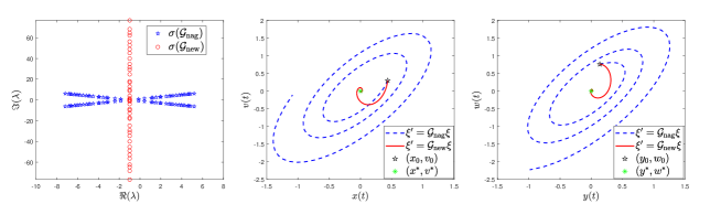
Figure 1: Numerical illustrations of the spectrum and the trajectories of 27 and 28.

Write $\mathcal{G}_{\rm new}=-I+\mathcal{L}+\mathcal{U}$, where $\mathcal{L}$ and $\mathcal{U}$ are respectively the strictly lower triangular and upper triangular part of $\mathcal{G}_{\rm new}$. Let $\alpha>0$ be the step size, we now consider the Gauss–Seidel splitting

$$\frac{\bm{\xi}_{k+1}-\bm{\xi}_{k}}{\alpha}=(-I+\mathcal{L})\bm{\xi}_{k+1}+\mathcal{U}\bm{\xi}_{k},$$ (31)

where the lower triangular part adopts the implicit discretization. A direct computation gives

$$\bm{\xi}_{k+1}=\widehat{\mathcal{G}}\bm{\xi}_{k},\quad\widehat{\mathcal{G}}=\left[(1+\alpha)I-\alpha\mathcal{L}\right]^{-1}\left(I+\alpha\mathcal{U}\right).$$

Theorem 3.1.

If $0<\alpha\leq 2\mu/\left\lVert{A}\right\rVert$, then $\rho(\widehat{\mathcal{G}})=\frac{1}{1+\alpha}$. In particular, taking $\alpha=\mu/\left\lVert{A}\right\rVert$ gives

$$\rho(\widehat{\mathcal{G}})=\frac{1}{1+\mu/\left\lVert{A}\right\rVert}.$$

Proof.

See Section A.2. ∎

Recall that for the unconstrained case 22, we see acceleration from $\mathcal{O}(1-1/\kappa(Q))$ to $\mathcal{O}(1-1/\sqrt{\kappa(Q)})$. For the quadratic game 25, it has $\mu\leq\Re(\lambda)$ and $\left\lvert{\lambda}\right\rvert\leq\sqrt{\mu^{2}+\left\lVert{A}\right\rVert^{2}}$ for all $\lambda\in\sigma(\mathcal{Q})$. From Theorem 3.1, we see a larger step size $\alpha=\mathcal{O}(\mu/\left\lVert{A}\right\rVert)$ leads to the improved spectral radius $\mathcal{O}(1-\mu/\left\lVert{A}\right\rVert)$, which is optimal [3, 35] and brings acceleration.

4 Continuous Model and Exponential Decay

4.1 Accelerated primal-dual hybrid gradient flow

Based on the template 28, we propose an accelerated primal-dual hybrid gradient (APDHG) flow:

$${}x^{\prime}=v-x,$$ (32a)

$${}y^{\prime}=w-y,$$ (32b)

$${}\gamma v^{\prime}\in{\mu_{\!f}}(x-v)-\partial_{x}\mathcal{L}(x,w),$$ (32c)

$${}\beta w^{\prime}\in{\mu_{g}}(y-w)+\partial_{y}\mathcal{L}(v,y).$$ (32d)

Here and in the sequel, the primal parameter $\gamma$ and the dual parameter $\beta$ satisfy

$$\gamma^{\prime}={\mu_{\!f}}-\gamma,\quad\beta^{\prime}={\mu_{g}}-\beta,$$ (33)

with arbitrary positive initial conditions. Eliminating the inertial variables $v$ and $w$ from 32d leads to a novel second-order ODE model

$${}\gamma x^{\prime\prime}+({\mu_{\!f}}+\gamma)x^{\prime}+\partial_{x}\mathcal{L}(x,y+y^{\prime})=0,$$ (34a)

$${}\beta y^{\prime\prime}+({\mu_{g}}+\beta)y^{\prime}-\partial_{y}\mathcal{L}(x+x^{\prime},y)=0.$$ (34b)

Under proper smooth setting, our APDHG flow 32d admits a unique global $C^{1}$-smooth solution $Z=(x,v,y,w):[0,\infty)\to\mathcal{Z}$. This allows us to establish the exponential decay property of the Lyapunov function along the continuous trajectory.

Theorem 4.1.

Assume $f/g$ are $C^{1}_{L_{f}}/C^{1}_{L_{g}}$-smooth and relatively $\mu_{f}/\mu_{g}$-convex with respect to $\phi/\psi$. There is a unique global $C^{1}$-smooth solution $Z:[0,\infty)\to\mathcal{Z}$ to the APDHG model 32d. Moreover, we have

$$\frac{\,{\rm d}}{\,{\rm d}t}\mathcal{E}(\Theta,Z;\widehat{z})\leq-\mathcal{E}(\Theta,Z;\widehat{z}),$$ (35)

where $\mathcal{E}(\Theta,Z;\widehat{z})$ is defined by 14 with any $\widehat{z}=(\widehat{x},\widehat{y})\in{\bf dom\,}\mathcal{L}$. This leads to the exponential decay

$$\mathcal{E}(\Theta(t),Z(t);\widehat{z})\leq e^{-t}\mathcal{E}(\Theta(0),Z(0);\widehat{z}),\quad\forall\,0<t<\infty.$$

Proof.

According to the Lipschitz assumption son $\nabla f$ and $\nabla g$, the right hand side of 32d is Lipschitz continuous over bounded sets. Thus, following the argument in [9, Theorem 4.1], we conclude that the unique $C^{1}$-smooth solution $Z=(x,v,y,w)$ exists globally on $[0,\infty)$.

It remains to establish 35. Invoking 32d and 33, a direct computation gives

$$\frac{\,{\rm d}}{\,{\rm d}t}\mathcal{E}(\Theta,Z;\widehat{z})=\left\langle{\nabla_{\Theta}\mathcal{E},\Theta^{\prime}}\right\rangle+\left\langle{\nabla_{Z}\mathcal{E},Z^{\prime}}\right\rangle:={} \mathbb{A}_{1}+\mathbb{A}_{2}+\mathbb{A}_{3}+\mathbb{A}_{4},$$ (36)

where

$$\left\{\begin{aligned} \mathbb{A}_{1}={}&\frac{{\mu_{\!f}}-\gamma}{2}\left\lVert{v-\widehat{x}}\right\rVert^{2}+\frac{{\mu_{g}}-\beta}{2}\left\lVert{w-\widehat{y}}\right\rVert^{2},\\ \mathbb{A}_{2}={}&{\mu_{\!f}}\left\langle{x-v,v-\widehat{x}}\right\rangle+{\mu_{g}}\left\langle{y-w,w-\widehat{y}}\right\rangle,\\ \mathbb{A}_{3}={}&\left\langle{\nabla_{y}\mathcal{L}(v,y),w-\widehat{y}}\right\rangle-\left\langle{\nabla_{y}\mathcal{L}(\widehat{x},y),w-y}\right\rangle,\\ \mathbb{A}_{4}={}&\left\langle{\nabla_{x}\mathcal{L}(x,\widehat{y}),v-x}\right\rangle-\left\langle{\nabla_{x}\mathcal{L}(x,w),v-\widehat{x}}\right\rangle.\end{aligned}\right.$$

Applying the three-term identity 9 gives that

$$\mathbb{A}_{2}={} \frac{{\mu_{\!f}}}{2}\left(\left\lVert{x-\widehat{x}}\right\rVert^{2}-\left\lVert{v-\widehat{x}}\right\rVert^{2}-\left\lVert{x-v}\right\rVert^{2}\right)$$

$$\quad+\frac{{\mu_{g}}}{2}\left(\left\lVert{y-\widehat{y}}\right\rVert^{2}-\left\lVert{w-\widehat{y}}\right\rVert^{2}-\left\lVert{y-w}\right\rVert^{2}\right).$$

For $\mathbb{A}_{3}$, by 12 and the strong convexity of $\widehat{g}(\cdot;\widehat{z})$, there follows

$$\mathbb{A}_{3}={} \left\langle{A(v-\widehat{x}),w-\widehat{y}}\right\rangle+\left\langle{\nabla_{y}\mathcal{L}(\widehat{x},y),w-\widehat{y}}\right\rangle-\left\langle{\nabla_{y}\mathcal{L}(\widehat{x},y),w-y}\right\rangle$$

$$={} \left\langle{A(v-\widehat{x}),w-\widehat{y}}\right\rangle+\left\langle{\nabla_{y}\mathcal{L}(\widehat{x},y),y-\widehat{y}}\right\rangle$$

$$={} \left\langle{A(v-\widehat{x}),w-\widehat{y}}\right\rangle-\left\langle{\nabla\widehat{g}(y),y-\widehat{y}}\right\rangle\quad\left(\text{by \lx@cref{creftype~refnum}{eq:subg}}\right)$$

$$\leq{} \left\langle{A(v-\widehat{x}),w-\widehat{y}}\right\rangle+g(\widehat{y})-\widehat{g}(y;\widehat{z})-\frac{{\mu_{g}}}{2}\left\lVert{y-\widehat{y}}\right\rVert^{2},$$

and similarly

$$\mathbb{A}_{4}\leq{} -\left\langle{A^{\top}(w-\widehat{y}),v-\widehat{x}}\right\rangle+f(\widehat{x})-\widehat{f}(x;\widehat{z})-\frac{{\mu_{\!f}}}{2}\left\lVert{x-\widehat{x}}\right\rVert^{2}.$$

This together with the fact 13 gives

$$\mathbb{A}_{3}+\mathbb{A}_{4}\leq{} g(\widehat{y})-\widehat{g}(y;\widehat{z})-\frac{{\mu_{g}}}{2}\left\lVert{y-\widehat{y}}\right\rVert^{2}+f(\widehat{x})-\widehat{f}(x;\widehat{z})-\frac{{\mu_{\!f}}}{2}\left\lVert{x-\widehat{x}}\right\rVert^{2}$$ (37)

$$= -\left(\mathcal{L}(x,\widehat{y})-\mathcal{L}(\widehat{x},y)\right)-\frac{{\mu_{g}}}{2}\left\lVert{y-\widehat{y}}\right\rVert^{2}-\frac{{\mu_{\!f}}}{2}\left\lVert{x-\widehat{x}}\right\rVert^{2}.$$

Therefore, combining this with $\mathbb{A}_{1}$ and $\mathbb{A}_{2}$ leads to

$$\frac{\,{\rm d}}{\,{\rm d}t}\mathcal{E}(\Theta,Z;\widehat{z})\leq -\mathcal{E}(\Theta,Z;\widehat{z})-\frac{{\mu_{g}}}{2}\left\lVert{y-w}\right\rVert^{2}-\frac{{\mu_{\!f}}}{2}\left\lVert{x-v}\right\rVert^{2}.$$

Using the substitutions $x^{\prime}=v-x$ and $y^{\prime}=w-y$, we obtain 35 and complete the proof. ∎

4.2 Accelerated Bregman primal-dual hybrid gradient flow

Motivated by the accelerated Bregman primal-dual flow [49] for solving linearly constrained optimization, to work with general non-Euclidean distances, we propose the following accelerated Bregman primal-dual hybrid gradient (AB-PDHG) flow:

$${}x^{\prime}=v-x,$$ (38a)

$${}y^{\prime}=w-y,$$ (38b)

$${}\gamma\frac{\,{\rm d}}{\,{\rm d}t}\nabla\phi(v)\in{\mu_{\!f}}(\nabla\phi(x)-\nabla\phi(v))-\partial_{x}\mathcal{L}(x,w),$$ (38c)

$${}\beta\frac{\,{\rm d}}{\,{\rm d}t}\nabla\psi(w)\in{\mu_{g}}(\nabla\phi(y)-\nabla\psi(w))+\partial_{y}\mathcal{L}(v,y),$$ (38d)

where $\gamma$ and $\beta$ are still governed by 33. Analogously to 34b, we can drop $v$ and $w$ to obtain

$${}\gamma\frac{\,{\rm d}}{\,{\rm d}t}\nabla\phi(x+x^{\prime})\in{\mu_{\!f}}(\nabla\phi(x)-\nabla\phi(x+x^{\prime}))-\partial_{x}\mathcal{L}(x,y+y^{\prime}),$$

$${}\beta\frac{\,{\rm d}}{\,{\rm d}t}\nabla\psi(y+y^{\prime})\in{\mu_{g}}(\nabla\phi(y)-\nabla\psi(y+y^{\prime}))+\partial_{y}\mathcal{L}(x+x^{\prime},y).$$

Remark 4.1.

Let us discuss the relation and difference among our models and existing works. We mainly focus on primal-dual dynamical systems for the saddle-point problem 1 and the equality constrained problem 4 with $Ax=b$, which is a special case of 1 with $g(y)=\left\langle{b,y}\right\rangle$.

• Linearly constrained problem 4: Looking at the equations for the primal variable and the dual variable (Lagrange multiplier), most works adopt either second-order + second-order [2, 10, 30, 80, 83] or first-order + first-order structures [15, 18, 47]. Besides, in [32, 46, 52, 49], the hybrid second-order + first-order combination has been considered. When $g(y)=\left\langle{b,y}\right\rangle$, both of our APDHG flow 34b and AB-PDHG flow 38d provide new second-order + second-order models for the equality constrained problem 4. Especially, the latter is equipped with general Bregman distances respectively for the primal variable and the Lagrange multiplier, which can be adapted to proper metrics and brings further preconditioning effect.

• Saddle-point problem 1: We are aware of some recent works [17, 29]. Compared with these, ours combine Bregman distances with subtlety time rescaling parameters for primal and dual variables. This paves the way for designing new (nonlinear) primal-dual splitting methods for both convex and (partially) strongly convex problems in a unified way.

Theorem 4.2.

Assume $(f,g)$ are $C^{1}$-smooth and relatively $(\mu_{f},\mu_{g})$-convex with respect to $(\phi,\psi)$. Let $Z=(x,v,y,w):[0,\infty)\to\mathcal{Z}$ be a global $C^{1}$-smooth solution to the ABPDHG flow 38d, then for the Lyapunov function 15, we have

$$\frac{\,{\rm d}}{\,{\rm d}t}\mathcal{E}_{D}(\Theta,Z;\widehat{z})\leq-\mathcal{E}_{D}(\Theta,Z;\widehat{z})-{\mu_{\!f}}D_{\psi}(v,x)-{\mu_{g}}D_{\psi}(w,y),$$ (39)

which implies

$$\mathcal{E}_{D}(\Theta(t),Z(t);\widehat{z})\leq e^{-t}\mathcal{E}_{D}(\Theta(0),Z(0);\widehat{z}),\quad\forall\,0<t<\infty,$$ (40)

for any $\widehat{z}=(\widehat{x},\widehat{y})\in{\bf dom\,}\mathcal{L}$.

Proof.

Observing Definition 2.2, a direct calculation gives

$$\frac{\,{\rm d}}{\,{\rm d}t}D_{\phi}(\widehat{x},v)=\left\langle{\frac{\,{\rm d}}{\,{\rm d}t}\nabla\phi(v),v-\widehat{x}}\right\rangle,\quad\frac{\,{\rm d}}{\,{\rm d}t}D_{\psi}(\widehat{y},w)=\left\langle{\frac{\,{\rm d}}{\,{\rm d}t}\nabla\psi(w),w-\widehat{y}}\right\rangle.$$

Therefore, similarly with 36, we take the time derivative on 38d and use the right hand side of 38d to obtain the expansion

$$\frac{\,{\rm d}}{\,{\rm d}t}\mathcal{E}_{D}(\Theta,Z;\widehat{z})={} \mathbb{A}_{1}+\mathbb{A}_{2}+\mathbb{A}_{3}+\mathbb{A}_{4},$$

where

$$\left\{\begin{aligned} \mathbb{A}_{1}={}&({\mu_{\!f}}-\gamma)D_{\phi}(\widehat{x},v)+({\mu_{g}}-\beta)D_{\psi}(\widehat{y},w),\\ \mathbb{A}_{2}={}&{\mu_{\!f}}\left\langle{\nabla\phi(x)-\nabla\phi(v),v-\widehat{x}}\right\rangle+{\mu_{g}}\left\langle{\nabla\psi(y)-\nabla\psi(w),w-\widehat{y}}\right\rangle,\\ \mathbb{A}_{3}={}&\left\langle{\nabla_{y}\mathcal{L}(v,y),w-\widehat{y}}\right\rangle-\left\langle{\nabla_{y}\mathcal{L}(\widehat{x},y),w-y}\right\rangle,\\ \mathbb{A}_{4}={}&\left\langle{\nabla_{x}\mathcal{L}(x,\widehat{y}),v-x}\right\rangle-\left\langle{\nabla_{x}\mathcal{L}(x,w),v-\widehat{x}}\right\rangle.\end{aligned}\right.$$

Following the proof of 35 and using the relatively strong convexity (cf.Definition 2.3), the estimate of $\mathbb{A}_{3}$ and $\mathbb{A}_{4}$ becomes (cf.37)

$$\mathbb{A}_{3}+\mathbb{A}_{4}\leq{} \mathcal{L}(\widehat{x},y)-\mathcal{L}(x,\widehat{y})-{\mu_{g}}D_{\psi}(\widehat{y},y)-{\mu_{\!f}}D_{\phi}(\widehat{x},x).$$

For the second term $\mathbb{A}_{2}$, applying Lemma 2.1 yields that

$$\mathbb{A}_{2}={} {\mu_{\!f}}\left(D_{\phi}(\widehat{x},x)-D_{\phi}(\widehat{x},v)-D_{\phi}(v,x)\right)+{\mu_{g}}\left(D_{\psi}(\widehat{y},y)-D_{\psi}(\widehat{y},w)-D_{\psi}(w,y)\right).$$

Consequently, collecting all the terms implies 39 and finishes the proof. ∎

Remark 4.2.

Since 40 holds for any $\widehat{z}=(\widehat{x},\widehat{y})\in{\bf dom\,}\mathcal{L}$, a further argument leads to the exponential convergence of the Lagrangian gap $\mathcal{L}(x(t),\widehat{y})-\mathcal{L}(\widehat{x},y(t))$ and the partial duality gap $\sup_{\widehat{z}\in X\times Y}\mathcal{L}(x(t),\widehat{y})-\mathcal{L}(\widehat{x},y(t))$ over any compact subset $X\times Y\subset{\bf dom\,}\mathcal{L}$. For simplicity, we omit the details.

5 Accelerated Bregman Primal-Dual Proximal Splitting

In this section, we propose an accelerated Bregman primal-dual proximal splitting for solving the saddle-point problem 1 under the following setting.

Assumption 2.

$(f,\,g)$ are relatively $(\mu_{f},\mu_{g})$-convex w.r.t. $(\phi,\psi)$ with ${\mu_{\!f}},{\mu_{g}}\geq 0$.

5.1 Discretization

Let us consider a semi-implicit Euler (SIE) scheme for the AB-PDHG flow system 38d. Given $Z_{k}=(x_{k},v_{k},y_{k},w_{k})\in\mathcal{Z}$ and $\Theta_{k}=(\gamma_{k},\beta_{k})\in\,{\mathbb{R}}_{+}^{2}$, find $\alpha_{k}>0$ and update $Z_{k+1}=(x_{k+1},v_{k+1},y_{k+1},w_{k+1})\in\mathcal{Z}$ by that

$${}\frac{x_{k+1}-x_{k}}{\alpha_{k}}=v_{k+1}-x_{k+1},$$ (41a)

$${}\frac{y_{k+1}-y_{k}}{\alpha_{k}}=\eta_{k}(w_{k+1}-y_{k+1}),$$ (41b)

$${}\gamma_{k}\frac{\nabla\phi(v_{k+1})-\nabla\phi(v_{k})}{\alpha_{k}}\in{\mu_{\!f}}(\nabla\phi(x_{k+1})-\nabla\phi(v_{k+1}))-\partial_{x}\mathcal{L}(x_{k+1},w_{k}),$$ (41c)

$${}\beta_{k}\frac{\nabla\psi(w_{k+1})-\nabla\psi(w_{k})}{\alpha_{k}}\in{\mu_{g}}(\nabla\psi(y_{k+1})-\nabla\psi(w_{k+1}))+\eta_{k}\partial_{y}\mathcal{L}({\bar{v}_{k+1}},y_{k+1}),$$ (41d)

where

$$\eta_{k}:=\frac{\alpha_{k+1}}{\alpha_{k}}(1+\alpha_{k}),\quad\bar{v}_{k+1}:=v_{k+1}+\frac{v_{k+1}-v_{k}}{\eta_{k}}.$$ (42)

To update $\Theta_{k+1}=(\gamma_{k+1},\beta_{k+1})\subset\,{\mathbb{R}}_{+}^{2}$, the continuous parameter equation 33 is discretized by

$$\frac{\gamma_{k+1}-\gamma_{k}}{\alpha_{k}}={}{\mu_{\!f}}-\gamma_{k+1},\quad\frac{\beta_{k+1}-\beta_{k}}{\alpha_{k}}={}{\mu_{g}}-\beta_{k+1},$$ (43)

with arbitrary positive initial values $\gamma_{0},\,\beta_{0}>0$. We mention that the factor $\eta_{k}\geq 1$ in (41b) and (41d) is actually a perturbation (cf.46) and $\bar{v}_{k+1}$ depends only on $v_{k}$ and $v_{k+1}$. Both two are chosen technically for the Lyapunov analysis in Section 5.2. Later in Algorithm 1, we reformulate the SIE scheme 41d as a primal-dual proximal splitting method.

5.2 Lyapunov analysis

In this part, we aim to establish the Lyapunov analysis of the SIE scheme 41d by using the discrete Lyapunov function $\mathcal{H}_{k}(\widehat{z})$ defined by 16. Motivated by the decomposition given in Lemma 2.5, in the next, we shall focus on $\mathbb{I}_{21}+\mathbb{I}_{22}$ and $\mathbb{I}_{31}+\mathbb{I}_{32}$ and prove the corresponding upper bounds separately in Lemmas 5.2 and 5.3.

Lemma 5.1.

Let $\{\gamma_{k}\}$ and $\{\beta_{k}\}$ be defined by 43 with any $\alpha_{k}>0$, then

$$\max\{\gamma_{0}\theta_{k},\,\min\{{\mu_{\!f}},\,\gamma_{0}\}\}\leq\gamma_{k}\leq\max\{{\mu_{\!f}},\,\gamma_{0}\},$$ (44a)

$$\max\{\beta_{0}\theta_{k},\,\min\{{\mu_{g}},\,\beta_{0}\}\}\leq\beta_{k}\leq\max\{{\mu_{g}},\,\beta_{0}\},$$ (44b)

where $\{\theta_{k}\}$ is defined by 20. If $\left\lVert{A}\right\rVert^{2}\alpha_{k}^{2}=(1-\chi)\gamma_{k}\beta_{k}$ with any $\chi\in[0,1)$, then $\eta_{k}=\alpha_{k+1}(1+\alpha_{k})/\alpha_{k}\geq 1$.

Proof.

By 43, we have

$$\gamma_{k+1}=\frac{{\mu_{\!f}}\alpha_{k}+\gamma_{k}}{1+\alpha_{k}},\quad\beta_{k+1}=\frac{{\mu_{g}}\alpha_{k}+\beta_{k}}{1+\alpha_{k}}.$$ (45)

In view of this and 21, a standard induction argument verifies 44. Furthermore, if $\left\lVert{A}\right\rVert^{2}\alpha_{k}^{2}=(1-\chi)\gamma_{k}\beta_{k}$, then it follows that

$$\eta_{k}={} \frac{1+\alpha_{k}}{\alpha_{k}}\alpha_{k+1}=\frac{1+\alpha_{k}}{\alpha_{k}\left\lVert{A}\right\rVert}\sqrt{(1-\chi)\gamma_{k+1}\beta_{k+1}}$$ (46)

$$={} \frac{\sqrt{1-\chi}}{\alpha_{k}\left\lVert{A}\right\rVert}\sqrt{({\mu_{\!f}}\alpha_{k}+\gamma_{k})({\mu_{g}}\alpha_{k}+\beta_{k})}$$

$$={} \frac{1}{\sqrt{\gamma_{k}\beta_{k}}}\sqrt{({\mu_{\!f}}\alpha_{k}+\gamma_{k})({\mu_{g}}\alpha_{k}+\beta_{k})}\geq 1.$$

This completes the proof of this lemma. ∎

Lemma 5.2.

Given $\Theta_{k}=(\gamma_{k},\beta_{k})\in\,{\mathbb{R}}_{+}^{2}$ and $Z_{k}=(x_{k},v_{k},y_{k},w_{k})\in\mathcal{Z}$, let $\Theta_{k+1}=(\gamma_{k+1},\beta_{k+1})\in\,{\mathbb{R}}_{+}^{2}$ and $Z_{k+1}=(x_{k+1},v_{k+1},y_{k+1},w_{k+1})\in\mathcal{Z}$ be the outputs of the SIE scheme 41d and the parameter equation 43 at the $k$-th step with any step size $\alpha_{k}>0$. Then we have

$$\mathbb{I}_{21}+\mathbb{I}_{22}\leq -\alpha_{k}\left\langle{A^{\top}(w_{k}-\widehat{y}),v_{k+1}-\widehat{x}}\right\rangle-\gamma_{k}D_{\phi}(v_{k+1},v_{k}),$$ (47)

where $\mathbb{I}_{21}$ and $\mathbb{I}_{22}$ are defined in 17 with any $\widehat{z}=(\widehat{x},\widehat{y})\in{\bf dom\,}\mathcal{L}$.

Proof.

According to Assumption 2, $f$ is relatively $\mu_{f}$-convex w.r.t. $\phi$ and so is $\widehat{f}(\cdot;\widehat{z})$ by Lemma 2.3 (i). This implies that

$$\mathbb{I}_{21}={} \widehat{f}(x_{k+1};\widehat{z})-\widehat{f}(x_{k};\widehat{z})+\alpha_{k}\left(\widehat{f}(x_{k+1};\widehat{z})-f(\widehat{x})\right)$$

$$\overset{\text{by \lx@cref{creftype~refnum}{eq:scv-f}}}{\leq} \left\langle{\partial\widehat{f}(x_{k+1};\widehat{z}),x_{k+1}-x_{k}}\right\rangle+\alpha_{k}\left\langle{\partial\widehat{f}(x_{k+1};\widehat{z}),x_{k+1}-\widehat{x}}\right\rangle-{\mu_{\!f}}\alpha_{k}D_{\phi}(\widehat{x},x_{k+1})$$

$$\overset{\text{by \eqref{eq:ab-pdps-x}}}{=} \alpha_{k}\left\langle{\partial\widehat{f}(x_{k+1};\widehat{z}),v_{k+1}-\widehat{x}}\right\rangle-{\mu_{\!f}}\alpha_{k}D_{\phi}(\widehat{x},x_{k+1}).$$ (48)

Notice that $\partial\widehat{f}(x_{k+1};\widehat{z})=\partial_{x}\mathcal{L}(x_{k+1},\widehat{y})=\partial_{x}\mathcal{L}(x_{k+1},w_{k})-A^{\top}(w_{k}-\widehat{y})$, which together with (41c) gives

$$\alpha_{k}\left\langle{\partial\widehat{f}(x_{k+1};\widehat{z}),v_{k+1}-\widehat{x}}\right\rangle$$

$$= -\alpha_{k}\left\langle{A^{\top}(w_{k}-\widehat{y}),v_{k+1}-\widehat{x}}\right\rangle+\gamma_{k}\left\langle{\nabla\phi(v_{k})-\nabla\phi(v_{k+1}),v_{k+1}-\widehat{x}}\right\rangle$$

$$\quad+{\mu_{\!f}}\alpha_{k}\left\langle{\nabla\phi(x_{k+1})-\nabla\phi(v_{k+1}),v_{k+1}-\widehat{x}}\right\rangle.$$

Plugging this into the previous estimate 48 and using the three-term identity 8, we obtain

$$\mathbb{I}_{21}\leq -{\mu_{\!f}}\alpha_{k}D_{\phi}(\widehat{x},x_{k+1})-\alpha_{k}\left\langle{A^{\top}(w_{k}-\widehat{y}),v_{k+1}-\widehat{x}}\right\rangle$$

$$\quad+\gamma_{k}\left(D_{\phi}(\widehat{x},v_{k})-D_{\phi}(\widehat{x},v_{k+1})-D_{\phi}(v_{k+1},v_{k})\right)$$

$$\qquad+{\mu_{\!f}}\alpha_{k}\left(D_{\phi}(\widehat{x},x_{k+1})-D_{\phi}(\widehat{x},v_{k+1})-D_{\phi}(v_{k+1},x_{k+1})\right)$$

$$= -{\mu_{\!f}}\alpha_{k}D_{\phi}(v_{k+1},x_{k+1})-\alpha_{k}\left\langle{A^{\top}(w_{k}-\widehat{y}),v_{k+1}-\widehat{x}}\right\rangle$$

$$\quad+\gamma_{k}D_{\phi}(\widehat{x},v_{k})-(\gamma_{k}+{\mu_{\!f}}\alpha_{k})D_{\phi}(\widehat{x},v_{k+1})-\gamma_{k}D_{\phi}(v_{k+1},v_{k}).$$

In view of 45, it follows that $\gamma_{k}+{\mu_{\!f}}\alpha_{k}=\gamma_{k+1}(1+\alpha_{k})$ and

$$\mathbb{I}_{21}\leq -\gamma_{k}D_{\phi}(v_{k+1},v_{k})-\alpha_{k}\left\langle{A^{\top}(w_{k}-\widehat{y}),v_{k+1}-\widehat{x}}\right\rangle$$

$$\quad-{\mu_{\!f}}\alpha_{k}D_{\phi}(v_{k+1},x_{k+1})+\underbrace{\gamma_{k}D_{\phi}(\widehat{x},v_{k})-\gamma_{k+1}(1+\alpha_{k})D_{\phi}(\widehat{x},v_{k+1})}_{=-\mathbb{I}_{22}}.$$

This implies 47 and completes the proof of this lemma. ∎

Lemma 5.3.

Given $\Theta_{k}=(\gamma_{k},\beta_{k})\in\,{\mathbb{R}}_{+}^{2}$ and $Z_{k}=(x_{k},v_{k},y_{k},w_{k})\in\mathcal{Z}$, let $\Theta_{k+1}=(\gamma_{k+1},\beta_{k+1})\in\,{\mathbb{R}}_{+}^{2}$ and $Z_{k+1}=(x_{k+1},v_{k+1},y_{k+1},w_{k+1})\in\mathcal{Z}$ be the outputs of the SIE scheme 41d and the parameter equation 43 with $\left\lVert{A}\right\rVert^{2}\alpha_{k}^{2}=(1-\chi)\gamma_{k}\beta_{k}$ and $\chi\in[0,1)$. Then we have

$$\mathbb{I}_{31}+\mathbb{I}_{32}\leq{} \alpha_{k}\eta_{k}\left\langle{A(\bar{v}_{k+1}-\widehat{x}),w_{k+1}-\widehat{y}}\right\rangle-\beta_{k}D_{\psi}(w_{k+1},w_{k}),$$ (49)

where $\mathbb{I}_{31}$ and $\mathbb{I}_{32}$ are defined in 17 with $\widehat{z}=(\widehat{x},\widehat{y})$ being a saddle point to 1.

Proof.

By Lemma 2.3 (ii) we have $\widehat{g}(y_{k+1};\widehat{z})\geq g(\widehat{y})$. Analogously to 48, using 10 and 2.3 (i) and (41b) implies that

$$\mathbb{I}_{31}={} \widehat{g}(y_{k+1};\widehat{z})-\widehat{g}(y_{k};\widehat{z})+\alpha_{k}\left(\widehat{g}(y_{k+1};\widehat{z})-g(\widehat{y})\right)$$

$$\leq{} \widehat{g}(y_{k+1};\widehat{z})-\widehat{g}(y_{k};\widehat{z})+\alpha_{k}\eta_{k}\left(\widehat{g}(y_{k+1};\widehat{z})-g(\widehat{y})\right)$$

$$\leq{} \left\langle{\partial\widehat{g}(y_{k+1};\widehat{z}),y_{k+1}-y_{k}}\right\rangle+\alpha_{k}\eta_{k}\left\langle{\partial\widehat{g}(y_{k+1};\widehat{z}),y_{k+1}-\widehat{y}}\right\rangle-{\mu_{g}}\alpha_{k}\eta_{k}D_{\psi}(\widehat{y},y_{k+1})$$

$$\leq{} \alpha_{k}\eta_{k}\left\langle{\partial\widehat{g}(y_{k+1};\widehat{z}),w_{k+1}-\widehat{y}}\right\rangle-{\mu_{g}}\alpha_{k}D_{\psi}(\widehat{y},y_{k+1}),$$

where in the second and the last lines, we used the fact $\eta_{k}\geq 1$, which holds true indeed by Lemma 5.1 and the step size condition $\left\lVert{A}\right\rVert^{2}\alpha_{k}^{2}=(1-\chi)\gamma_{k}\beta_{k}$. Observing that $\partial\widehat{g}(y_{k+1};\widehat{z})=\partial_{y}\mathcal{L}(\bar{v}_{k+1},y_{k+1})+A(\bar{v}_{k+1}-\widehat{x})$, we get

$$\mathbb{I}_{31}\overset{\text{by \eqref{eq:ab-pdps-w}}}{\leq} -{\mu_{g}}\alpha_{k}D_{\psi}(\widehat{y},y_{k+1})+\alpha_{k}\eta_{k}\left\langle{A(\bar{v}_{k+1}-\widehat{x}),w_{k+1}-\widehat{y}}\right\rangle$$

$$\quad+{\mu_{g}}\alpha_{k}\left(D_{\psi}(\widehat{y},y_{k+1})-D_{\psi}(\widehat{y},w_{k+1})-D_{\psi}(w_{k+1},y_{k+1})\right)$$

$$\qquad+\beta_{k}\left(D_{\psi}(\widehat{y},w_{k})-D_{\psi}(\widehat{y},w_{k+1})-D_{\psi}(w_{k+1},w_{k})\right)$$

$$\overset{\text{by \lx@cref{creftype~refnum}{eq:3-id}}}{=} -{\mu_{g}}\alpha_{k}D_{\psi}(w_{k+1},y_{k+1})+\alpha_{k}\eta_{k}\left\langle{A(\bar{v}_{k+1}-\widehat{x}),w_{k+1}-\widehat{y}}\right\rangle$$

$$\quad+\underbrace{\beta_{k}D_{\psi}(\widehat{y},w_{k})-(\beta_{k}+{\mu_{g}}\alpha_{k})D_{\psi}(\widehat{y},w_{k+1})}_{=-\mathbb{I}_{32}}-\beta_{k}D_{\psi}(w_{k+1},w_{k}).$$

We mention that $\beta_{k}+{\mu_{g}}\alpha_{k}=\beta_{k+1}(1+\alpha_{k})$ (cf.45). This finishes the proof of 49. ∎

Theorem 5.1.

Given $\Theta_{k}=(\gamma_{k},\beta_{k})\in\,{\mathbb{R}}_{+}^{2}$ and $Z_{k}=(x_{k},v_{k},y_{k},w_{k})\in\mathcal{Z}$, let $\Theta_{k+1}=(\gamma_{k+1},\beta_{k+1})\in\,{\mathbb{R}}_{+}^{2}$ and $Z_{k+1}=(x_{k+1},v_{k+1},y_{k+1},w_{k+1})\in\mathcal{Z}$ be the outputs of the SIE scheme 41d and the parameter equation 43 with $\left\lVert{A}\right\rVert^{2}\alpha_{k}^{2}=(1-\chi)\gamma_{k}\beta_{k}$ and $\chi\in[0,1)$. Then we have

$$\mathcal{H}_{k+1}(\widehat{z})-\mathcal{H}_{k}(\widehat{z})+\alpha_{k}\mathcal{H}_{k+1}(\widehat{z})\leq{}-\chi\left(\frac{\gamma_{k}}{2}\left\lVert{v_{k+1}-v_{k}}\right\rVert^{2}+\frac{\beta_{k}}{2}\left\lVert{w_{k+1}-w_{k}}\right\rVert^{2}\right),$$ (50)

where $\mathcal{H}_{k}(\widehat{z})$ is define by 16 with $\widehat{z}=(\widehat{x},\widehat{y})$ being a saddle point to 1.

Proof.

Thanks to Lemmas 5.2 and 5.3 and the decomposition 17, we obtain

$$\mathcal{H}_{k+1}(\widehat{z})-\mathcal{H}_{k}(\widehat{z})+\alpha_{k}\mathcal{H}_{k+1}(\widehat{z})\leq{} \Delta_{k}-\gamma_{k}D_{\phi}(v_{k},v_{k+1})-\beta_{k}D_{\psi}(w_{k},w_{k+1}),$$ (51)

where

$$\Delta_{k}={} \alpha_{k}\eta_{k}\left\langle{A(\bar{v}_{k+1}-\widehat{x}),w_{k+1}-\widehat{y}}\right\rangle-\alpha_{k}\left\langle{A(v_{k+1}-\widehat{x}),w_{k}-\widehat{y}}\right\rangle$$ (52)

$$\quad+\alpha_{k}\left\langle{A(v_{k}-\widehat{x}),w_{k}-\widehat{y}}\right\rangle-\alpha_{k+1}(1+\alpha_{k})\left\langle{A(v_{k+1}-\widehat{x}),w_{k+1}-\widehat{y}}\right\rangle.$$

Recalling 42, we expand the first term as follows

$$\alpha_{k}\eta_{k}\left\langle{A(\bar{v}_{k+1}-\widehat{x}),w_{k+1}-\widehat{y}}\right\rangle=\alpha_{k+1}(1+\alpha_{k})\left\langle{A(\bar{v}_{k+1}-\widehat{x}),w_{k+1}-\widehat{y}}\right\rangle$$

$$={} \alpha_{k}\eta_{k}\left\langle{A(v_{k+1}-\widehat{x}),w_{k+1}-\widehat{y}}\right\rangle+\alpha_{k}\left\langle{A(v_{k+1}-v_{k}),w_{k+1}-\widehat{y}}\right\rangle,$$

which yields that $\Delta_{k}=\alpha_{k}\left\langle{A(v_{k+1}-v_{k}),w_{k+1}-w_{k}}\right\rangle$. Hence, using the fact $\left\lVert{A}\right\rVert^{2}\alpha_{k}^{2}=(1-\chi)\gamma_{k}\beta_{k}$ and the mean value inequality gives

$$\Delta_{k}\leq(1-\chi)\left(\frac{\gamma_{k}}{2}\left\lVert{v_{k+1}-v_{k}}\right\rVert^{2}+\frac{\beta_{k}}{2}\left\lVert{w_{k+1}-w_{k}}\right\rVert^{2}\right).$$

In view of 51 and the $1$-strongly convex property of the prox-functions (cf.Definition 2.1), we obtain 50 and conclude the proof of this theorem. ∎

5.3 The overall algorithm and iteration complexity

The overall SIE scheme 41d with the step size condition $\left\lVert{A}\right\rVert^{2}\alpha_{k}^{2}\leq\gamma_{k}\beta_{k}$ is listed in Algorithm 1, which is called the Accelerated Bregman Primal Dual Proximal Splitting (AB-PDPS). By Assumption 2, the objectives of the proximal steps in Lines 7 and 11 of Algorithm 1 are (strongly) convex.

Algorithm 1 AB-PDPS for solving 1 under Assumptions 1 and 2

0:  Problem parameters: ${\mu_{\!f}},\,{\mu_{g}}\geq 0$ and $\left\lVert{A}\right\rVert$.     Initial guesses: $x_{0},v_{0}\in{\bf dom\,}f$ and $y_{0},w_{0}\in{\bf dom\,}g$.    Initial parameters: $\gamma_{0},\,\beta_{0}>0$.

1:  for $k=0,1,\ldots$ do

2:     Take $\alpha_{k}\leq\sqrt{\gamma_{k}\beta_{k}}/\left\lVert{A}\right\rVert$.

3:     Update $\gamma_{k+1}=({\mu_{\!f}}\alpha_{k}+\gamma_{k})/(1+\alpha_{k})$ and $\beta_{k+1}=({\mu_{g}}\alpha_{k}+\beta_{k})/(1+\alpha_{k})$.

4:     Compute $\alpha_{k+1}=\sqrt{\gamma_{k+1}\beta_{k+1}}/\left\lVert{A}\right\rVert$ and $\eta_{k}=\alpha_{k+1}(1+\alpha_{k})/\alpha_{k}$.

5:     

6:     Define $f_{k}(x,v):=f(x)+\gamma_{k+1}D_{\phi}(v,v_{k})+\left\langle{A^{\top}w_{k},x}\right\rangle$.

7:     Update $x_{k+1}=\mathop{{\mathop{{\rm argmin}}\,}}\limits_{x\in\,{\mathbb{R}}^{n}}\left\{f_{k}(x,v)-{\mu_{\!f}}D_{\phi}(x,v_{k}):\,v=x+\frac{x-x_{k}}{\alpha_{k}}\right\}$.

8:     Update $v_{k+1}=x_{k+1}+(x_{k+1}-x_{k})/\alpha_{k}$ and $\bar{v}_{k+1}=v_{k+1}+(v_{k+1}-v_{k})/\eta_{k}$.

9:     

10:     Define $g_{k}(y,w):=g(y)+\frac{1+\alpha_{k}}{1+\alpha_{k}\eta_{k}}\beta_{k+1}D_{\psi}(w,w_{k})-\left\langle{A\bar{v}_{k+1},y}\right\rangle$.

11:     Update $y_{k+1}=\mathop{{\mathop{{\rm argmin}}\,}}\limits_{y\in\,{\mathbb{R}}^{m}}\left\{\eta_{k}g_{k}(y,w)-{\mu_{g}}D_{\psi}(y,w_{k}):\,w=y+\frac{y-y_{k}}{\alpha_{k}\eta_{k}}\right\}$.

12:     Update $w_{k+1}=y_{k+1}+(y_{k+1}-y_{k})/(\alpha_{k}\eta_{k})$.

13:  end for

Remark 5.1.

Let $R\in\,{\mathbb{R}}^{n\times n}$ and $S\in\,{\mathbb{R}}^{m\times m}$ be SPD. If we choose quadratic prox-functions

$$\phi(x)=1/2\left\lVert{x}\right\rVert_{R}^{2},\quad\psi(y)=1/2\left\lVert{y}\right\rVert_{S}^{2},$$ (53)

then the proximal steps in Lines 7 and 11 become

$$x_{k+1}={} \mathop{{\mathop{{\rm argmin}}\,}}\limits_{x\in\,{\mathbb{R}}^{n}}\!\!\left\{f(x)+\left\langle{A^{\top}w_{k},x}\right\rangle+\frac{\delta_{k}}{2\alpha_{k}^{2}}\left\lVert{x-\widetilde{x}_{k}}\right\rVert_{R}^{2}\right\},$$ (54)

$$y_{k+1}={} \mathop{{\mathop{{\rm argmin}}\,}}\limits_{y\in\,{\mathbb{R}}^{m}}\!\!\left\{g(y)-\left\langle{A\bar{v}_{k+1},y}\right\rangle+\frac{\tau_{k}}{2\eta_{k}\alpha_{k}^{2}}\left\lVert{y-\widetilde{y}_{k}}\right\rVert_{S}^{2}\right\},$$ (55)

where

$$\delta_{k}={} {\mu_{\!f}}\alpha_{k}+\gamma_{k}(1+\alpha_{k}),{} \widetilde{x}_{k}=\frac{1}{\delta_{k}}\left(({\mu_{\!f}}\alpha_{k}+\gamma_{k})x_{k}+\gamma_{k}\alpha_{k}v_{k}\right),$$

$$\tau_{k}={} {\mu_{g}}\alpha_{k}+\beta_{k}(1+\eta_{k}\alpha_{k}),{} \widetilde{y}_{k}=\frac{1}{\tau_{k}}(({\mu_{g}}\alpha_{k}+\beta_{k})y_{k}+\eta_{k}\beta_{k}\alpha_{k}w_{k}).$$

Theorem 5.2.

Assume that $\{(x_{k},y_{k})\}\subset{\bf dom\,}\mathcal{L}$ is generated by Algorithm 1 with $\left\lVert{A}\right\rVert^{2}\alpha_{k}^{2}=(1-\chi)\gamma_{k}\beta_{k}$ and $\chi\in[0,1)$. Then we have

$$\left\{\begin{aligned} {}&\mathcal{L}(x_{k},\widehat{y})-\mathcal{L}(\widehat{x},y_{k})+\frac{{\mu_{\!f}}}{2}\left\lVert{x_{k}-\widehat{x}}\right\rVert^{2}+\frac{{\mu_{g}}}{2}\left\lVert{y_{k}-\widehat{y}}\right\rVert^{2}\leq 2\theta_{k}\mathcal{H}_{0}(\widehat{z}),\\ {}&\sum_{i=0}^{k-1}\frac{\chi}{\theta_{i}}\left(\gamma_{i}\left\lVert{v_{i+1}-v_{i}}\right\rVert^{2}+\beta_{i}\left\lVert{w_{i+1}-w_{i}}\right\rVert^{2}\right)\leq 4\mathcal{H}_{0}(\widehat{z}),\end{aligned}\right.$$ (56)

where $\{\theta_{k}\}$ is defined by 20 and $\widehat{z}=(\widehat{x},\widehat{y})$ a saddle point to 1. Moreover, if $\gamma_{0}\geq{\mu_{\!f}},\,\beta_{0}\geq{\mu_{g}}$ and $\gamma_{0}\beta_{0}\leq\left\lVert{A}\right\rVert^{2}$, then

$$\theta_{k}\leq{} \min\left\{\frac{\|\widehat{A}\|}{\sqrt{\gamma_{0}\beta_{0}}k},\,\frac{64\|\widehat{A}\|^{2}}{{\mu_{g}}\gamma_{0}k^{2}},\,\frac{64\|\widehat{A}\|^{2}}{{\mu_{\!f}}\beta_{0}k^{2}},\,\left(1+\frac{1-\chi}{\sqrt{\kappa_{P}}}\right)^{-k}\right\},$$ (57)

for all $k\geq 1$, where $\kappa_{P}=\left\lVert{A}\right\rVert^{2}/({\mu_{\!f}}{\mu_{g}})$ and $\widehat{A}=A/(1-\chi)$.

Proof.

Applying Lemmas 2.5 and 5.1 proves 56. Recall the difference equation 21 of $\{\theta_{k}\}$.

To establish 57, the key is to find the upper bound and lower bound of $\alpha_{k}$. Since $\gamma_{0}\geq{\mu_{\!f}}$ and $\beta_{0}\geq{\mu_{g}}$, by 44 we have $\gamma_{k}\leq\gamma_{0}$ and $\beta_{k}\leq\beta_{0}$, which implies

$$\alpha_{k}=\frac{\sqrt{1-\chi}}{\left\lVert{A}\right\rVert}\sqrt{\gamma_{k}\beta_{k}}=\sqrt{\gamma_{k}\beta_{k}}/\|\widehat{A}\|\leq\sqrt{\gamma_{0}\beta_{0}}/\left\lVert{A}\right\rVert\leq 1.$$

The lower bound of $\alpha_{k}$ is more subtle. From 44, both $\gamma_{k}$ and $\beta_{k}$ have two under estimates. Hence, we consider four situations.

• First of all, for $\alpha_{k}\geq\sqrt{\gamma_{0}\beta_{0}}\theta_{k}/\|\widehat{A}\|=\alpha_{0}\theta_{k}$, it follows from 21 that $\theta_{k+1}-\theta_{k}\leq-\alpha_{0}\theta_{k}\theta_{k+1}$. This also implies $1/\theta_{k+1}-1/\theta_{k}\geq\alpha_{0}$ and yields that $\theta_{k}\leq 1/(1+\alpha_{0}k)\leq\|\widehat{A}\|/(\sqrt{\gamma_{0}\beta_{0}}k)$.

• Secondly, for $\alpha_{k}\geq\sqrt{{\mu_{\!f}}\beta_{0}\theta_{k}}/\|\widehat{A}\|$, we have $\theta_{k+1}-\theta_{k}\leq-\sqrt{{\mu_{\!f}}\beta_{0}}\sqrt{\theta_{k}}\theta_{k+1}/\|\widehat{A}\|$. Notice that $\theta_{k+1}/\theta_{k}=1/(1+\alpha_{k})\geq 1/(1+\alpha_{0})\geq 1/2$. Hence, invoking Lemma C.1 implies $\theta_{k}\leq 64\|\widehat{A}\|^{2}/({\mu_{\!f}}\beta_{0}k^{2})$.

• Similarly, for $\alpha_{k}\geq\sqrt{{\mu_{g}}\gamma_{0}\theta_{k}}/\|\widehat{A}\|$, we get $\theta_{k}\leq 64\|\widehat{A}\|^{2}/({\mu_{g}}\gamma_{0}k^{2})$.

• Finally, for $\alpha_{k}\geq\sqrt{{\mu_{\!f}}{\mu_{g}}}/\|\widehat{A}\|=(1-\chi)/\sqrt{\kappa_{P}}$, we obtain from 20 that $\theta_{k}\leq\left(1+(1-\chi)/\sqrt{\kappa_{P}}\right)^{-k}$.

Note that these estimates hold simultaneously. This leads to 57 and finishes the proof. ∎

According to convergence rate estimate 57, we conclude that Algorithm 1 admits the optimal iteration complexity [64, 81] under the proximal algorithm class [81, Definition 2.1] $(x_{k},y_{k})\in\mathcal{X}^{k}\times\mathcal{Y}^{k}$, where

$$\left\{\begin{aligned} \mathcal{X}^{k+1}:={}&{\bf span}\left\{x_{i},\,{\bf prox}_{\delta_{i}f}(\widetilde{x}_{i}-\delta_{i}A^{\top}\widetilde{y}_{i}):\,\widetilde{x}_{i}\in\mathcal{X}^{i},\widetilde{y}_{i}\in\mathcal{Y}^{i},\,0\leq i\leq k\right\},\\ \mathcal{Y}^{k+1}:={}&{\bf span}\left\{y_{i},\,{\bf prox}_{\tau_{i}g}(\widetilde{y}_{i}+\tau_{i}A\widetilde{x}_{i}):\,\widetilde{x}_{i}\in\mathcal{X}^{i},\widetilde{y}_{i}\in\mathcal{Y}^{i},\,0\leq i\leq k\right\},\end{aligned}\right.$$

with $\mathcal{X}^{0}:={\bf span}\left\{x_{0}\right\}$ and $\mathcal{Y}^{0}:={\bf span}\left\{y_{0}\right\}$. More precisely, to achieve the accuracy $\mathcal{L}(x_{k},\widehat{y})-\mathcal{L}(\widehat{x},y_{k})\leq\epsilon$, the iteration complexity is

$$\mathcal{O}\left(\min\left\{\frac{\left\lVert{A}\right\rVert}{\epsilon},\,\frac{\left\lVert{A}\right\rVert}{\sqrt{{\mu_{\!f}}\epsilon}},\,\frac{\left\lVert{A}\right\rVert}{\sqrt{{\mu_{g}}\epsilon}},\,\sqrt{\kappa_{P}}\left\lvert{\ln\epsilon}\right\rvert\right\}\right).$$

When ${\mu_{\!f}}>0$, the iteration complexity for finding $\left\lVert{x_{k}-\widehat{x}}\right\rVert^{2}\leq\epsilon$ is

$$\mathcal{O}\left(\min\left\{\frac{\left\lVert{A}\right\rVert}{{\mu_{\!f}}\sqrt{\epsilon}},\,\sqrt{\kappa_{P}}\left\lvert{\ln\frac{{\mu_{\!f}}}{\epsilon}}\right\rvert\right\}\right).$$

When ${\mu_{g}}>0$, the iteration complexity for finding $\left\lVert{y_{k}-\widehat{y}}\right\rVert^{2}\leq\epsilon$ is

$$\mathcal{O}\left(\min\left\{\frac{\left\lVert{A}\right\rVert}{{\mu_{g}}\sqrt{\epsilon}},\,\sqrt{\kappa_{P}}\left\lvert{\ln\frac{{\mu_{g}}}{\epsilon}}\right\rvert\right\}\right).$$

Remark 5.2.

Thanks to the second estimate in 56, we have fast convergence results on $\{v_{k+1}-v_{k}\}$ and $\{w_{k+1}-w_{k}\}$. In view of Lemma 5.1, we have $\gamma_{k}\geq\theta_{k}\gamma_{0}$ and $\beta_{k}\geq\theta_{k}\beta_{0}$. Putting this into 56 implies

$$\sum_{k=0}^{\infty}\left(\gamma_{0}\left\lVert{v_{k+1}-v_{k}}\right\rVert^{2}+\beta_{0}\left\lVert{w_{k+1}-w_{k}}\right\rVert^{2}\right)<\infty,$$

which gives $\left\lVert{v_{k+1}-v_{k}}\right\rVert^{2}=o\left(1/k\right)$ and $\left\lVert{w_{k+1}-w_{k}}\right\rVert^{2}=o\left(1/k\right)$. If ${\mu_{\!f}}>0$, then by 57 we have

$$\sum_{k=0}^{\infty}\left(\frac{\mu_{f}^{2}}{\|\widehat{A}\|^{2}}k^{2}\left\lVert{v_{k+1}-v_{k}}\right\rVert^{2}+\left\lVert{w_{k+1}-w_{k}}\right\rVert^{2}\right)<\infty.$$

This gives the fast convergence $\left\lVert{v_{k+1}-v_{k}}\right\rVert^{2}=o\left(1/k^{3}\right)$. Similarly, for ${\mu_{g}}>0$, we also have $\left\lVert{w_{k+1}-w_{k}}\right\rVert^{2}=o\left(1/k^{3}\right)$. If ${\mu_{\!f}}{\mu_{g}}>0$, then it follows from 57 that

$$\sum_{k=0}^{\infty}\left(1+\frac{1-\chi}{\sqrt{\kappa_{P}}}\right)^{k}\left({\mu_{\!f}}\left\lVert{v_{k+1}-v_{k}}\right\rVert^{2}+{\mu_{g}}\left\lVert{w_{k+1}-w_{k}}\right\rVert^{2}\right)<\infty.$$

6 Accelerated Bregman Primal-Dual Proximal Gradient Splitting

In this section, we mainly focus on the composite case $f=f_{1}+f_{2}$ with the smooth + nonsmooth structure that satisfies the following setting.

Assumption 3.

$g$ is relatively $\mu_{g}$-convex w.r.t. $\psi$ and $f=f_{1}+f_{2}$ where $f_{1}$ is $C_{{L_{\!f}}}^{1}$-smooth and relatively $\mu_{f}$-convex w.r.t. $\phi$.

6.1 Algorithm and Lyapunov analysis

Based on 41d, we propose an variant SIE scheme for the continuous AB-PDHG flow model 38d. Given $Z_{k}=(x_{k},v_{k},y_{k},w_{k})\in\mathcal{Z}$ and $\Theta_{k}=(\gamma_{k},\beta_{k})\in\,{\mathbb{R}}_{+}^{2}$, find $\alpha_{k}>0$ and update $Z_{k+1}=(x_{k+1},v_{k+1},y_{k+1},w_{k+1})\in\mathcal{Z}$ as follows

$${}\frac{x_{k+1}-x_{k}}{\alpha_{k}}=v_{k+1}-x_{k+1},$$ (58a)

$${}\frac{y_{k+1}-y_{k}}{\alpha_{k}}=\eta_{k}(w_{k+1}-y_{k+1}),$$ (58b)

$${}\gamma_{k}\frac{\nabla\phi(v_{k+1})-\nabla\phi(v_{k})}{\alpha_{k}}\in{\mu_{\!f}}(\nabla\phi(\bar{x}_{k})-\nabla\phi(v_{k+1}))-\mathcal{F}(\bar{x}_{k},w_{k},v_{k+1}),$$ (58c)

$${}\beta_{k}\frac{\nabla\psi(w_{k+1})-\nabla\psi(w_{k})}{\alpha_{k}}\in{\mu_{g}}(\nabla\psi(y_{k+1})-\nabla\psi(w_{k+1}))+\eta_{k}\partial_{y}\mathcal{L}({\bar{v}_{k+1}},y_{k+1}),$$ (58d)

where $\eta_{k}$ and $\bar{v}_{k+1}$ is defined by 42 and

$$\mathcal{F}(\bar{x}_{k},w_{k},v_{k+1})=\nabla f_{1}(\bar{x}_{k})+\partial f_{2}(v_{k+1})+A^{\top}w_{k},\quad\bar{x}_{k}=\frac{x_{k}+\alpha_{k}v_{k}}{1+\alpha_{k}}.$$

Notice that (58b) and (58d) are identical to (41b) and (41d) respectively. The parameter updating template 43 leaves unchanged, but the third step (58c) differs from (41c) since we replace $\partial_{x}\mathcal{L}(x_{k+1},w_{k})=\partial f(x_{k+1})+A^{\top}w_{k}$ with $\mathcal{F}(\bar{x}_{k},w_{k},v_{k+1})$.

With the step size condition $({L_{\!f}}\beta_{k}+\left\lVert{A}\right\rVert^{2})\alpha_{k}^{2}\leq\gamma_{k}\beta_{k}$, we rearrange 58d as a primal-dual proximal gradient method and summarize it in Algorithm 2, which is called Accelerated Bregman Primal-Dual Proximal Gradient Splitting (AB-PDPGS).

Algorithm 2 AB-PDPGS for solving 1 under Assumptions 1 and 3

0:  Problem parameters: ${\mu_{\!f}},\,{\mu_{g}}\geq 0,\,{L_{\!f}}$ and $\left\lVert{A}\right\rVert$.     Initial guesses: $x_{0},v_{0}\in{\bf dom\,}f$ and $y_{0},w_{0}\in{\bf dom\,}g$.    Initial parameters: $\gamma_{0},\,\beta_{0}>0$.

1:  for $k=0,1,\ldots$ do

2:     Take $\alpha_{k}\leq\sqrt{\gamma_{k}\beta_{k}/({L_{\!f}}\beta_{k}+\left\lVert{A}\right\rVert^{2})}$.

3:     Update $\gamma_{k+1}=({\mu_{\!f}}\alpha_{k}+\gamma_{k})/(1+\alpha_{k})$ and $\beta_{k+1}=({\mu_{g}}\alpha_{k}+\beta_{k})/(1+\alpha_{k})$.

4:     Compute $\alpha_{k+1}=\sqrt{\gamma_{k+1}\beta_{k+1}/({L_{\!f}}\beta_{k+1}+\left\lVert{A}\right\rVert^{2})}$ and $\eta_{k}=\alpha_{k+1}(1+\alpha_{k})/\alpha_{k}$.

5:     

6:     Set $\widetilde{v}_{k}=\nabla f_{1}(\bar{x}_{k})+A^{\top}w_{k}-{\mu_{\!f}}(\nabla\phi(\bar{x}_{k})-\nabla\phi(v_{k}))$.

7:     Update $v_{k+1}=\mathop{{\mathop{{\rm argmin}}\,}}\limits_{v\in\,{\mathbb{R}}^{n}}\!\!\left\{f_{2}(v)+\left\langle{\widetilde{v}_{k},v}\right\rangle+\frac{\gamma_{k}+{\mu_{\!f}}\alpha_{k}}{\alpha_{k}}D_{\phi}(v,v_{k})\right\}$.

8:     Update $x_{k+1}=(x_{k}+\alpha_{k}v_{k+1})/(1+\alpha_{k})$ and $\bar{v}_{k+1}=v_{k+1}+(v_{k+1}-v_{k})/\eta_{k}$.

9:     

10:     Define $g_{k}(y,w):=g(y)+\frac{1+\alpha_{k}}{1+\alpha_{k}\eta_{k}}\beta_{k+1}D_{\psi}(w,w_{k})-\left\langle{A\bar{v}_{k+1},y}\right\rangle$.

11:     Update $y_{k+1}=\mathop{{\mathop{{\rm argmin}}\,}}\limits_{y\in\,{\mathbb{R}}^{m}}\left\{\eta_{k}g_{k}(y,w)-{\mu_{g}}D_{\psi}(y,w_{k}):\,w=y+\frac{y-y_{k}}{\alpha_{k}\eta_{k}}\right\}$.

12:     Update $w_{k+1}=y_{k+1}+(y_{k+1}-y_{k})/(\alpha_{k}\eta_{k})$.

13:  end for

Remark 6.1.

As discussed in 5.1, if we choose 53, then the subproblems in Algorithm 2 agree with standard preconditioned proximal calculations. Indeed, the minimization problem in Line 11 coincides with 55 while the proximal step in Line 7 becomes

$$v_{k+1}=\mathop{{\mathop{{\rm argmin}}\,}}\limits_{v\in\,{\mathbb{R}}^{n}}\!\!\left\{f_{2}(v)+\left\langle{\widetilde{v}_{k},v}\right\rangle+\frac{\gamma_{k}+{\mu_{\!f}}\alpha_{k}}{2\alpha_{k}}\left\lVert{v-v_{k}}\right\rVert_{R}^{2}\right\}.$$ (59)

Lemma 6.1.

Let $\{\Theta_{k}=(\gamma_{k},\beta_{k})\}\subset\,{\mathbb{R}}_{+}^{2}$ and $\{Z_{k}=(x_{k},v_{k},y_{k},w_{k})\}\subset\mathcal{Z}$ be generated by Algorithm 2. It holds that

$$\mathbb{I}_{21}+\mathbb{I}_{22}\leq -\alpha_{k}\left\langle{A^{\top}(w_{k}-\widehat{y}),v_{k+1}-\widehat{x}}\right\rangle-\gamma_{k}D_{\phi}(v_{k+1},v_{k})+\frac{L_{f}\alpha_{k}^{2}}{2(1+\alpha_{k})}\left\lVert{v_{k+1}-v_{k}}\right\rVert^{2},$$ (60)

where $\mathbb{I}_{21}$ and $\mathbb{I}_{22}$ are defined in 17 with any $\widehat{z}=(\widehat{x},\widehat{y})\in{\bf dom\,}\mathcal{L}$.

Proof.

In view of 11 and (58a), it holds that

$$\mathbb{I}_{21}={} f(x_{k+1})-f(x_{k})+\alpha_{k}\left(f(x_{k+1})-f(\widehat{x})\right)$$

$$\quad+\left\langle{A^{\top}\widehat{y},x_{k+1}-x_{k}}\right\rangle+\alpha_{k}\left\langle{A^{\top}\widehat{y},x_{k+1}-\widehat{x}}\right\rangle$$

$$={} f(x_{k+1})-f(x_{k})+\alpha_{k}\left(f(x_{k+1})-f(\widehat{x})\right)+\alpha_{k}\left\langle{A^{\top}\widehat{y},v_{k+1}-\widehat{x}}\right\rangle.$$

Since $f=f_{1}+f_{2}$, let us establish the upper bounds for $f_{1}$ and $f_{2}$ separately. By Assumptions 3 and 2.2, we have

$$\alpha_{k}\left(f_{1}(x_{k+1})-f_{1}(\widehat{x})\right)+f_{1}(x_{k+1})-f_{2}(x_{k})$$

$$\leq{} \alpha_{k}\left(\left\langle{\nabla f_{1}(\bar{x}_{k}),x_{k+1}-\widehat{x}}\right\rangle-{\mu_{\!f}}D_{\phi}(\widehat{x},\bar{x}_{k})+\frac{L_{f}}{2}\left\lVert{x_{k+1}-\bar{x}_{k}}\right\rVert^{2}\right)$$

$$\quad+\left\langle{\nabla f_{1}(\bar{x}_{k}),x_{k+1}-x_{k}}\right\rangle+\frac{L_{f}}{2}\left\lVert{x_{k+1}-\bar{x}_{k}}\right\rVert^{2}$$

$$\overset{\text{by \eqref{eq:ab-pdpgs-x}}}{=}{} \alpha_{k}\left\langle{\nabla f_{1}(\bar{x}_{k}),v_{k+1}-\widehat{x}}\right\rangle-{\mu_{\!f}}\alpha_{k}D_{\phi}(\widehat{x},\bar{x}_{k})+\frac{L_{f}(1+\alpha_{k})}{2}\left\lVert{x_{k+1}-\bar{x}_{k}}\right\rVert^{2}.$$ (61)

For the nonsmooth part $f_{2}$, we use convexity to obtain

$$\alpha_{k}\left(f_{2}(x_{k+1})-f_{2}(\widehat{x})\right)+f_{2}(x_{k+1})-f_{2}(x_{k})$$

$$\overset{\text{by \eqref{eq:ab-pdpgs-x} }}{=}{} \alpha_{k}\left(f_{2}\left(\frac{x_{k}+\alpha_{k}v_{k+1}}{1+\alpha_{k}}\right)-f_{2}(\widehat{x})\right)+f_{2}\left(\frac{x_{k}+\alpha_{k}v_{k+1}}{1+\alpha_{k}}\right)-f_{2}(x_{k})$$

$$\leq{} \alpha_{k}\left(\frac{1}{1+\alpha_{k}}f_{2}(x_{k})+\frac{\alpha_{k}}{1+\alpha_{k}}f_{2}(v_{k+1})-f_{2}(\widehat{x})\right)$$

$$\quad+\frac{1}{1+\alpha_{k}}f_{2}(x_{k})+\frac{\alpha_{k}}{1+\alpha_{k}}f_{2}(v_{k+1})-f_{2}(x_{k})$$

$$={} \alpha_{k}\left(f_{2}(v_{k+1})-f_{2}(\widehat{x})\right).$$

Observing (58c), we find $p_{k+1}\in\partial f_{2}(v_{k+1})$, where

$$p_{k+1}:=\gamma_{k}\frac{\nabla\phi(v_{k})-\nabla\phi(v_{k+1})}{\alpha_{k}}+{\mu_{\!f}}(\nabla\phi(\bar{x}_{k})-\nabla\phi(v_{k+1}))-\nabla f_{1}(\bar{x}_{k})-A^{\top}w_{k}.$$

Hence, it follows immediately that

$$\alpha_{k}\left(f_{2}(x_{k+1})-f_{2}(\widehat{x})\right)+f_{2}(x_{k+1})-f_{2}(x_{k})\leq{}\alpha_{k}\left\langle{p_{k+1},v_{k+1}-\widehat{x}}\right\rangle$$ (62)

$$={} \gamma_{k}\left\langle{\nabla\phi(v_{k})-\nabla\phi(v_{k+1}),v_{k+1}-\widehat{x}}\right\rangle+{\mu_{\!f}}\alpha_{k}\left\langle{\nabla\phi(\bar{x}_{k})-\nabla\phi(v_{k+1}),v_{k+1}-\widehat{x}}\right\rangle$$

$$\quad-\alpha_{k}\left\langle{\nabla f_{1}(\bar{x}_{k})+A^{\top}w_{k},v_{k+1}-\widehat{x}}\right\rangle.$$

Applying Lemma 2.1 gives

$${\mu_{\!f}}\alpha_{k}\left\langle{\nabla\phi(\bar{x}_{k})-\nabla\phi(v_{k+1}),v_{k+1}-\widehat{x}}\right\rangle={} {\mu_{\!f}}\alpha_{k}\left(D_{\phi}(\widehat{x},\bar{x}_{k})-D_{\phi}(\widehat{x},v_{k+1})-D_{\phi}(v_{k+1},\bar{x}_{k})\right),$$

$$\gamma_{k}\left\langle{\nabla\phi(v_{k})-\nabla\phi(v_{k+1}),v_{k+1}-\widehat{x}}\right\rangle={} \gamma_{k}\left(D_{\phi}(\widehat{x},v_{k})-D_{\phi}(\widehat{x},v_{k+1})-D_{\phi}(v_{k+1},v_{k})\right).$$

Combining this with 61 and 62, we get

$$\mathbb{I}_{21}\leq -\gamma_{k}D_{\phi}(v_{k+1},v_{k})+\frac{L_{f}(1+\alpha_{k})}{2}\left\lVert{x_{k+1}-\bar{x}_{k}}\right\rVert^{2}-\alpha_{k}\left\langle{A^{\top}(w_{k}-\widehat{y}),v_{k+1}-\widehat{x}}\right\rangle$$

$$\quad-{\mu_{\!f}}\alpha_{k}D_{\phi}(v_{k+1},\bar{x}_{k})+\underbrace{\gamma_{k}D_{\phi}(\widehat{x},v_{k})-(\gamma_{k}+\mu_{f}\alpha_{k})D_{\phi}(\widehat{x},v_{k+1})}_{=-\mathbb{I}_{22}}.$$

In view of (58a) and the setting $\bar{x}_{k}=(x_{k}+\alpha_{k}v_{k})/(1+\alpha_{k})$, we have $x_{k+1}-\bar{x}_{k}=\alpha_{k}(v_{k+1}-v_{k})/(1+\alpha_{k})$. Since $\gamma_{k}+{\mu_{\!f}}\alpha_{k}=\gamma_{k+1}(1+\alpha_{k})$, we can move the second line to the left hand side to get 60. This completes the proof of this lemma. ∎

Theorem 6.1.

Let $\{\Theta_{k}=(\gamma_{k},\beta_{k})\}\subset\,{\mathbb{R}}_{+}^{2}$ and $\{Z_{k}=(x_{k},v_{k},y_{k},w_{k})\}\subset\mathcal{Z}$ be generated by Algorithm 2. If $\beta_{0}\geq\mu_{g}$ and $({L_{\!f}}\beta_{k}+\left\lVert{A}\right\rVert^{2})\alpha_{k}^{2}=(1-\chi)^{2}\gamma_{k}\beta_{k}$ with $\chi\in[0,1)$, then it holds that

$$\mathcal{H}_{k+1}(\widehat{z})-\mathcal{H}_{k}(\widehat{z})+\alpha_{k}\mathcal{H}_{k+1}(\widehat{z})\leq-\chi\left(\frac{\beta_{k}}{2}\left\lVert{w_{k+1}-w_{k}}\right\rVert^{2}+\frac{\gamma_{k}}{2}\left\lVert{v_{k+1}-v_{k}}\right\rVert^{2}\right),$$ (63)

where $\mathcal{H}_{k}(\widehat{z})$ is define by 16 with $\widehat{z}=(\widehat{x},\widehat{y})$ being a saddle point to 1.

Proof.

Similar with Lemma 5.1, the lower bound $\eta_{k}\geq 1$ still holds true. Indeed, since $\beta_{0}\geq{\mu_{g}}$, by 45 and 44, it follows that $\beta_{k}\geq\beta_{k+1}\geq\mu_{g}$ and

$$\eta_{k}=\frac{1+\alpha_{k}}{\alpha_{k}}\alpha_{k+1}={} \frac{1+\alpha_{k}}{\alpha_{k}}\frac{\sqrt{(1-\chi)\gamma_{k+1}\beta_{k+1}}}{\sqrt{{L_{\!f}}\beta_{k+1}+\left\lVert{A}\right\rVert^{2}}}\geq\sqrt{1-\chi}\frac{\sqrt{({\mu_{\!f}}\alpha_{k}+\gamma_{k})({\mu_{g}}\alpha_{k}+\beta_{k})}}{\alpha_{k}\sqrt{{L_{\!f}}\beta_{k}+\left\lVert{A}\right\rVert^{2}}}$$

$$={} \sqrt{\left(1+{\mu_{\!f}}\alpha_{k}/\gamma_{k}\right)\left(1+{\mu_{g}}\alpha_{k}/\beta_{k}\right)}\geq 1.$$

Compared with 41d, we see that (41b) = (58b) and (41d) = (58d). Also, both 41d and 58d share with the same settings in 42 and 43. Hence, we conclude that the estimate 49 leaves unchanged:

$$\mathbb{I}_{31}+\mathbb{I}_{32}\leq{} \alpha_{k}\eta_{k}\left\langle{A(\bar{v}_{k+1}-\widehat{y}),w_{k+1}-\widehat{y}}\right\rangle-\beta_{k}D_{\psi}(w_{k+1},w_{k}).$$

Collecting this with 17 and 6.1 yields that

$$\mathcal{H}_{k+1}(\widehat{z})-\mathcal{H}_{k}(\widehat{z})+\alpha_{k}\mathcal{H}_{k+1}(\widehat{z})$$ (64)

$$\leq{} \Delta_{k}+\frac{L_{f}\alpha_{k}^{2}}{2(1+\alpha_{k})}\left\lVert{v_{k+1}-v_{k}}\right\rVert^{2}-\gamma_{k}D_{\phi}(v_{k},v_{k+1})-\beta_{k}D_{\psi}(w_{k},w_{k+1}),$$

where $\Delta_{k}$ is defined by 52 and can be further estimated as follows

$$\Delta_{k}\overset{\text{by \lx@cref{creftype~refnum}{eq:etak-b-vk1}}}{=}{} \alpha_{k}\left\langle{A(v_{k+1}-v_{k}),w_{k+1}-w_{k}}\right\rangle$$

$$\leq{} {}\frac{(1-\chi)\beta_{k}}{2}\left\lVert{w_{k+1}-w_{k}}\right\rVert^{2}+\frac{\left\lVert{A}\right\rVert^{2}\alpha_{k}^{2}}{2\beta_{k}(1-\chi)}\left\lVert{v_{k+1}-v_{k}}\right\rVert^{2}.$$

Since $({L_{\!f}}\beta_{k}+\left\lVert{A}\right\rVert^{2})\alpha_{k}^{2}=(1-\chi)^{2}\gamma_{k}\beta_{k}$, we claim that

$$\frac{\left\lVert{A}\right\rVert^{2}}{\beta_{k}(1-\chi)}+\frac{L_{f}}{1+\alpha_{k}}\leq\frac{\left\lVert{A}\right\rVert^{2}+L_{f}\beta_{k}}{\beta_{k}(1-\chi)}=\frac{\gamma_{k}(1-\chi)}{\alpha_{k}^{2}},$$

which implies

$$\Delta_{k}+\frac{L_{f}\alpha_{k}^{2}}{2(1+\alpha_{k})}\left\lVert{v_{k+1}-v_{k}}\right\rVert^{2}\leq{}(1-\chi)\left(\frac{\beta_{k}}{2}\left\lVert{w_{k+1}-w_{k}}\right\rVert^{2}+\frac{\gamma_{k}}{2}\left\lVert{v_{k+1}-v_{k}}\right\rVert^{2}\right).$$

Plugging this into 64 leads to the desired result 63 and finishes the proof. ∎

6.2 Convergence rate and iteration complexity

Theorem 6.2.

Assume that $\{(x_{k},y_{k})\}\subset{\bf dom\,}\mathcal{L}$ is generated by Algorithm 2 with $({L_{\!f}}\beta_{k}+\left\lVert{A}\right\rVert^{2})\alpha_{k}^{2}=(1-\chi)^{2}\gamma_{k}\beta_{k}$ and $\chi\in[0,1)$. Then we have

$$\left\{\begin{aligned} {}&\mathcal{L}(x_{k},\widehat{y})-\mathcal{L}(\widehat{x},y_{k})+\frac{{\mu_{\!f}}}{2}\left\lVert{x_{k}-\widehat{x}}\right\rVert^{2}+\frac{{\mu_{g}}}{2}\left\lVert{y_{k}-\widehat{y}}\right\rVert^{2}\leq 2\theta_{k}\mathcal{H}_{0}(\widehat{z}),\\ {}&\sum_{i=0}^{k-1}\frac{\chi}{\theta_{i}}\left(\gamma_{i}\left\lVert{v_{i+1}-v_{i}}\right\rVert^{2}+\beta_{i}\left\lVert{w_{i+1}-w_{i}}\right\rVert^{2}\right)\leq 4\mathcal{H}_{0}(\widehat{z}),\end{aligned}\right.$$ (65)

where $\{\theta_{k}\}$ is defined by 20 and $\widehat{z}=(\widehat{x},\widehat{y})$ a saddle point to 1. Moreover, if $\gamma_{0}\geq\mu_{f},\,\beta_{0}\geq{\mu_{g}}$ and $\gamma_{0}\beta_{0}\leq{L_{\!f}}\beta_{0}+\left\lVert{A}\right\rVert^{2}$, then we have two decay estimates for $\theta_{k}$.

• If ${\mu_{\!f}}={\mu_{g}}=0$, then it holds that

  $$\theta_{k}\leq\frac{64\widehat{{L_{\!f}}}}{\gamma_{0}k^{2}}+\frac{4\|\widehat{A}\|}{\sqrt{\gamma_{0}\beta_{0}}k},$$ (66)

  where $\widehat{{L_{\!f}}}={L_{\!f}}/(1-\chi)^{2}$ and $\widehat{A}=A/(1-\chi)^{2}$.

• If ${\mu_{\!f}}+{\mu_{g}}>0$, then we have

  $$\theta_{k}\leq\min\left\{\exp\left(-\frac{(1-\chi)k}{4\sqrt{\kappa_{\!f_{1}}}}\right)+\frac{64\|\widehat{A}\|^{2}}{{\mu_{\!f}}\beta_{0}k^{2}},\,\frac{64\widehat{{L_{\!f}}}}{\gamma_{0}k^{2}}+\frac{64\|\widehat{A}\|^{2}}{{\mu_{g}}\gamma_{0}k^{2}}\right\},$$ (67)

  where $\kappa_{\!f_{1}}={L_{\!f}}/{\mu_{\!f}}$.

• If ${\mu_{\!f}}{\mu_{g}}>0$, then

  $$\theta_{k}\leq\left(1+\frac{1-\chi}{\sqrt{\kappa_{P}+\kappa_{\!f_{1}}}}\right)^{-k},$$ (68)

  where $\kappa_{P}=\left\lVert{A}\right\rVert^{2}/({\mu_{\!f}}{\mu_{g}})$.

Proof.

Since $\left\lVert{A}\right\rVert^{2}\alpha_{k}^{2}\leq\gamma_{k}\beta_{k}$ (cf. Line 2 of Algorithm 2), applying Lemmas 2.5 and 6.1 proves 65. Let us establish the decay rate of $\theta_{k}$, which satisfies the difference equation 21. By 44, we have $\gamma_{k}\leq\gamma_{0}$ and $\beta_{k}\leq\beta_{0}$ and thus

$$\alpha_{k}=\frac{(1-\chi)\sqrt{\gamma_{k}\beta_{k}}}{\sqrt{{L_{\!f}}\beta_{k}+\left\lVert{A}\right\rVert^{2}}}=\frac{\sqrt{\gamma_{k}\beta_{k}}}{\sqrt{\widehat{{L_{\!f}}}\beta_{k}+\|\widehat{A}\|^{2}}}\leq\frac{\sqrt{\gamma_{0}\beta_{0}}}{\sqrt{{L_{\!f}}\beta_{0}+\left\lVert{A}\right\rVert^{2}}}\leq 1.$$

Similarly with the proof of 57, according to the lower bounds of $\gamma_{k}$ and $\beta_{k}$, we consider four scenarios.

• Firstly, for $\alpha_{k}\geq\sqrt{\gamma_{0}\beta_{0}}\theta_{k}/\sqrt{\widehat{{L_{\!f}}}\beta_{0}\theta_{k}+\|\widehat{A}\|^{2}}$, we have

  $$\theta_{k+1}-\theta_{k}\,\overset{\text{ by \lx@cref{creftype~refnum}{eq:diff-tk}}}{\leq}\,-\frac{\sqrt{\gamma_{0}\beta_{0}}\theta_{k}\theta_{k+1}}{\sqrt{\widehat{{L_{\!f}}}\beta_{0}\theta_{k}+\|\widehat{A}\|^{2}}}\,\overset{\text{ by \lx@cref{creftype~refnum}{lem:app-est}}}{\Longrightarrow}\,\theta_{k}\leq\frac{64\widehat{{L_{\!f}}}}{\gamma_{0}k^{2}}+\frac{4\|\widehat{A}\|}{\sqrt{\gamma_{0}\beta_{0}}k}.$$

• Secondly, for $\alpha_{k}\geq\sqrt{{\mu_{\!f}}\beta_{0}\theta_{k}}/\sqrt{\widehat{{L_{\!f}}}\beta_{0}\theta_{k}+\|\widehat{A}\|^{2}}$, it follows from 21 that

  $$\theta_{k+1}-\theta_{k}\leq-\frac{\sqrt{{\mu_{\!f}}\beta_{0}\theta_{k}}\theta_{k+1}}{\sqrt{\widehat{{L_{\!f}}}\beta_{0}\theta_{k}+\|\widehat{A}\|^{2}}}\,\overset{\text{ by \lx@cref{creftype~refnum}{lem:app-est}}}{\Longrightarrow}\,\theta_{k}\leq\exp\left(-\frac{k}{4}\sqrt{\frac{{\mu_{\!f}}}{\widehat{{L_{\!f}}}}}\right)+\frac{64\|\widehat{A}\|^{2}}{{\mu_{\!f}}\beta_{0}k^{2}}.$$

• Thirdly, for $\alpha_{k}\geq\sqrt{{\mu_{g}}\gamma_{0}\theta_{k}}/\sqrt{\widehat{{L_{\!f}}}{\mu_{g}}+\|\widehat{A}\|^{2}}$, applying Lemma C.1 once gain gives

  $$\theta_{k+1}-\theta_{k}\,\overset{\text{ by \lx@cref{creftype~refnum}{eq:diff-tk}}}{\leq}\,-\frac{\sqrt{{\mu_{g}}\gamma_{0}\theta_{k}}\theta_{k+1}}{\sqrt{\widehat{{L_{\!f}}}{\mu_{g}}+\|\widehat{A}\|^{2}}}\,\overset{\text{ by \lx@cref{creftype~refnum}{lem:app-est}}}{\Longrightarrow}\,\theta_{k}\leq\frac{64\widehat{{L_{\!f}}}}{\gamma_{0}k^{2}}+\frac{64\|\widehat{A}\|^{2}}{{\mu_{g}}\gamma_{0}k^{2}}.$$

• Finally, for $\alpha_{k}\geq\sqrt{{\mu_{\!f}}{\mu_{g}}}/\sqrt{\widehat{{L_{\!f}}}{\mu_{g}}+\|\widehat{A}\|^{2}}$, it follows from 20 that

  $$\theta_{k}\leq\left(1+\frac{\sqrt{{\mu_{\!f}}{\mu_{g}}}}{\sqrt{\widehat{{L_{\!f}}}{\mu_{g}}+\|\widehat{A}\|^{2}}}\right)^{-k}.$$

Note that the above four estimates hold simultaneously for $\theta_{k}$. Particularly, the first one (i) proves 67 and combining the second (ii) and the third (iii) implies 67, and the last one gives 68. This finishes the proof of this theorem. ∎

Similarly with the discussion in 5.2, from Theorem 6.2 we have fast convergence results on $\{v_{k+1}-v_{k}\}$ and $\{w_{k+1}-w_{k}\}$. Besides, we claim that Algorithm 2 admits the optimal iteration complexity [64, 81]. Specifically, to obtain $\mathcal{L}(x_{k},\widehat{y})-\mathcal{L}(\widehat{x},y_{k})\leq\epsilon$, the iteration complexity is

$$\mathcal{O}\left(\min\left\{\frac{\left\lVert{A}\right\rVert}{\epsilon}+\frac{\sqrt{{L_{\!f}}}}{\epsilon},\,\frac{\left\lVert{A}\right\rVert}{\sqrt{{\mu_{\!f}}\epsilon}}+\sqrt{\kappa_{\!f_{1}}}\left\lvert{\ln\epsilon}\right\rvert,\,\frac{\left\lVert{A}\right\rVert}{\sqrt{{\mu_{g}}\epsilon}}+\frac{\sqrt{{L_{\!f}}}}{\epsilon},\,\sqrt{\kappa_{P}}\left\lvert{\ln\epsilon}\right\rvert\right\}\right).$$

When ${\mu_{\!f}}>0$, the iteration complexity for finding $\left\lVert{x_{k}-\widehat{x}}\right\rVert^{2}\leq\epsilon$ is

$$\mathcal{O}\left(\min\left\{\frac{\left\lVert{A}\right\rVert}{{\mu_{\!f}}\sqrt{\epsilon}},\,\sqrt{\kappa_{P}}\left\lvert{\ln\frac{{\mu_{\!f}}}{\epsilon}}\right\rvert\right\}+\sqrt{\kappa_{\!f_{1}}}\left\lvert{\ln\frac{{\mu_{\!f}}}{\epsilon}}\right\rvert\right).$$

When ${\mu_{g}}>0$, the iteration complexity for finding $\left\lVert{y_{k}-\widehat{y}}\right\rVert^{2}\leq\epsilon$ is

$$\mathcal{O}\left(\min\left\{\frac{\left\lVert{A}\right\rVert}{{\mu_{g}}\sqrt{\epsilon}}+\sqrt{\frac{{L_{\!f}}}{{\mu_{g}}\epsilon}},\,\sqrt{\kappa_{P}+\kappa_{\!f_{1}}}\left\lvert{\ln\frac{{\mu_{g}}}{\epsilon}}\right\rvert\right\}\right).$$

7 A Symmetric AB-PDPGS Method

In this part, we following the last section and further consider the case that both $f$ and $g$ possess the smooth + nonsmooth composite structure.

Assumption 4.

$f=f_{1}+f_{2}$ where $f_{1}$ is $C_{{L_{\!f}}}^{1}$-smooth and relatively strongly convex w.r.t. $\phi$ with ${\mu_{\!f}}\geq 0$. $g=g_{1}+g_{2}$ where $g_{1}$ is $C_{L_{g}}^{1}$-smooth and relatively strongly convex w.r.t. $\psi$ with ${\mu_{g}}\geq 0$.

7.1 Algorithm presentation and Lyapunov analysis

We propose a symmetric version of the previous SIE scheme 58d:

$${}\frac{x_{k+1}-x_{k}}{\alpha_{k}}=v_{k+1}-x_{k+1},$$ (69a)

$${}\frac{y_{k+1}-y_{k}}{\alpha_{k}}=\eta_{k}(w_{k+1}-y_{k+1}),$$ (69b)

$${}\gamma_{k}\frac{\nabla\phi(v_{k+1})-\nabla\phi(v_{k})}{\alpha_{k}}\in{\mu_{\!f}}(\nabla\phi(\bar{x}_{k})-\nabla\phi(v_{k+1}))-\mathcal{F}(\bar{x}_{k},w_{k},v_{k+1}),$$ (69c)

$${}\beta_{k}\frac{\nabla\psi(w_{k+1})-\nabla\psi(w_{k})}{\alpha_{k}}\in{\mu_{g}}(\nabla\psi(\bar{y}_{k})-\nabla\psi(w_{k+1}))-\eta_{k}\mathcal{G}(\bar{y}_{k},\bar{v}_{k+1},w_{k+1}),$$ (69d)

where $\eta_{k}$ and $\bar{v}_{k+1}$ are defined by 42 and

$$\mathcal{F}(\bar{x}_{k},w_{k},v_{k+1})={} \nabla f_{1}(\bar{x}_{k})+\partial f_{2}(v_{k+1})+A^{\top}w_{k},\quad\bar{x}_{k}=\frac{x_{k}+\alpha_{k}v_{k}}{1+\alpha_{k}},$$

$$\mathcal{G}(\bar{y}_{k},\bar{v}_{k+1},w_{k+1})={} \nabla g_{1}(\bar{y}_{k})+\partial g_{2}(w_{k+1})-A\bar{v}_{k+1},\quad\bar{y}_{k}=\frac{y_{k}+\eta_{k}\alpha_{k}w_{k}}{1+\eta_{k}\alpha_{k}}.$$

Similarly with 58d, the parameter updating relation 43 leaves unchanged.

We take the step size $\alpha_{k}^{2}(L_{f}\beta_{k}+L_{g}\gamma_{k}+\left\lVert{A}\right\rVert^{2})=\gamma_{k}\beta_{k}$ and rearrange 69d as a primal-dual proximal gradient splitting method and list it below in Algorithm 3, which is called the Symmetric Accelerated Bregman Primal-Dual Proximal Gradient Splitting (Symmetric AB-PDPGS for short).

Remark 7.1.

As discussed in 6.1, when we choose 53, the subproblems in Algorithm 3 reduce to standard preconditioned proximal steps. In this case, the inner problem in Line 7 agrees with 59 and the proximal problem in Line 11 becomes

$$w_{k+1}=\mathop{{\mathop{{\rm argmin}}\,}}\limits_{w\in\,{\mathbb{R}}^{m}}\!\!\left\{g_{2}(w)+\left\langle{\nabla g_{1}(\bar{y}_{k})-A\bar{v}_{k+1}-\widetilde{w}_{k},w}\right\rangle+\frac{\beta_{k}+{\mu_{g}}\alpha_{k}}{2\alpha_{k}\eta_{k}}\left\lVert{w-w_{k}}\right\rVert_{S}^{2}\right\}.$$

Algorithm 3 Symmetric AB-PDPGS for solving 1 under Assumptions 1 and 4

0:  Problem parameters: ${\mu_{\!f}},\,{\mu_{g}}\geq 0,\,L_{f},\,L_{g}$ and $\left\lVert{A}\right\rVert$.     Initial guesses: $x_{0},v_{0}\in{\bf dom\,}f$ and $y_{0},w_{0}\in{\bf dom\,}g$.    Initial parameters: $\gamma_{0},\,\beta_{0}>0$.

1:  for $k=0,1,\ldots$ do

2:     Compute $\alpha_{k}=\sqrt{\gamma_{k}\beta_{k}/(L_{f}\beta_{k}+L_{g}\gamma_{k}+\left\lVert{A}\right\rVert^{2})}$.

3:     Update $\gamma_{k+1}=({\mu_{\!f}}\alpha_{k}+\gamma_{k})/(1+\alpha_{k})$ and $\beta_{k+1}=({\mu_{g}}\alpha_{k}+\beta_{k})/(1+\alpha_{k})$.

4:     Set $\alpha_{k+1}=\sqrt{\gamma_{k+1}\beta_{k+1}/(L_{f}\beta_{k+1}+L_{g}\gamma_{k+1}+\left\lVert{A}\right\rVert^{2})}$ and $\eta_{k}=\frac{\alpha_{k+1}}{\alpha_{k}}(1+\alpha_{k})$.

5:     

6:     Set $\widetilde{v}_{k}=\nabla f_{1}(\bar{x}_{k})+A^{\top}w_{k}-{\mu_{\!f}}(\nabla\phi(\bar{x}_{k})-\nabla\phi(v_{k}))$.

7:     Update $v_{k+1}=\mathop{{\mathop{{\rm argmin}}\,}}\limits_{v\in\,{\mathbb{R}}^{n}}\!\!\left\{f_{2}(v)+\left\langle{\widetilde{v}_{k},v}\right\rangle+\frac{\gamma_{k}+{\mu_{\!f}}\alpha_{k}}{\alpha_{k}}D_{\phi}(v,v_{k})\right\}$.

8:     Update $x_{k+1}=(x_{k}+\alpha_{k}v_{k+1})/(1+\alpha_{k})$ and $\bar{v}_{k+1}=v_{k+1}+(v_{k+1}-v_{k})/\eta_{k}$.

9:     

10:     Set $\widetilde{w}_{k}=\nabla g_{1}(\bar{y}_{k})-A\bar{v}_{k+1}-{\mu_{g}}/\eta_{k}(\nabla\psi(\bar{y}_{k})-\nabla\psi(w_{k}))$.

11:     Update $w_{k+1}=\mathop{{\mathop{{\rm argmin}}\,}}\limits_{w\in\,{\mathbb{R}}^{m}}\!\!\left\{g_{2}(w)+\left\langle{\widetilde{w}_{k},w}\right\rangle+\frac{\beta_{k}+{\mu_{g}}\alpha_{k}}{\eta_{k}\alpha_{k}}D_{\psi}(w,w_{k})\right\}$.

12:     Update $y_{k+1}=(y_{k}+\alpha_{k}\eta_{k}w_{k+1})/(1+\alpha_{k}\eta_{k})$.

13:  end for

Lemma 7.1.

Let $\{\Theta_{k}=(\gamma_{k},\beta_{k})\}\subset\,{\mathbb{R}}_{+}^{2}$ and $\{Z_{k}=(x_{k},v_{k},y_{k},w_{k})\}\subset\mathcal{Z}$ be generated by Algorithm 3. If $\gamma_{0}\geq\mu_{f}$ and $\beta_{0}\geq\mu_{g}$, then we have

$$\mathbb{I}_{31}+\mathbb{I}_{32}\leq{} \alpha_{k}\eta_{k}\left\langle{A(\bar{v}_{k+1}-\widehat{x}),w_{k+1}-\widehat{y}}\right\rangle-\beta_{k}D_{\psi}(w_{k+1},w_{k})+\frac{L_{g}\alpha_{k}^{2}\eta_{k}^{2}}{2(1+\alpha_{k}\eta_{k})}\left\lVert{w_{k+1}-w_{k}}\right\rVert^{2},$$ (70)

where $\mathbb{I}_{31}$ and $\mathbb{I}_{32}$ are defined in 17 with $\widehat{z}=(\widehat{x},\widehat{y})$ being a saddle point to 1.

Proof.

By Lemma 2.3 (ii) we have $\widehat{g}(y_{k+1};\widehat{z})\geq g(\widehat{y})$. Since $\alpha_{k}^{2}(L_{f}\beta_{k}+L_{g}\gamma_{k}+\left\lVert{A}\right\rVert^{2})=\gamma_{k}\beta_{k}$, using 45 gives

$$\eta_{k}={} \frac{1+\alpha_{k}}{\alpha_{k}}\alpha_{k+1}=\frac{1+\alpha_{k}}{\alpha_{k}}\frac{\sqrt{\gamma_{k+1}\beta_{k+1}}}{\sqrt{L_{f}\beta_{k+1}+L_{g}\gamma_{k+1}+\left\lVert{A}\right\rVert^{2}}}$$

$$\geq{} \frac{\sqrt{(\gamma_{k}+{\mu_{\!f}}\alpha_{k})(\beta_{k}+{\mu_{g}}\alpha_{k})}}{\alpha_{k}\sqrt{L_{f}\beta_{k}+L_{g}\gamma_{k}+\left\lVert{A}\right\rVert^{2}}}={}\sqrt{\left(1+{\mu_{\!f}}\alpha_{k}/\gamma_{k}\right)\left(1+{\mu_{g}}\alpha_{k}/\beta_{k}\right)}\geq 1.$$

Above, we used the monotone relations $\gamma_{k}\geq\gamma_{k+1}$ and $\beta_{k}\geq\beta_{k+1}$, which holds true by 44 and our assumption: $\gamma_{0}\geq\mu_{f}$ and $\beta_{0}\geq\mu_{g}$. Following the proof of Lemma 6.1, we shall split $g=g_{1}+g_{2}$ into two parts. For the sake of completeness, we provide the detailed proof in Appendix B. ∎

Theorem 7.1.

Let $\{\Theta_{k}=(\gamma_{k},\beta_{k})\}\subset\,{\mathbb{R}}_{+}^{2}$ and $\{Z_{k}=(x_{k},v_{k},y_{k},w_{k})\}\subset\mathcal{Z}$ be generated by Algorithm 3. If $\gamma_{0}\geq\mu_{f}$ and $\beta_{0}\geq\mu_{g}$, then we have

$$\mathcal{H}_{k+1}(\widehat{z})-\mathcal{H}_{k}(\widehat{z})+\alpha_{k}\mathcal{H}_{k+1}(\widehat{z})\leq 0,$$ (71)

where $\mathcal{H}_{k}(\widehat{z})$ is define by 16 with $\widehat{z}=(\widehat{x},\widehat{y})$ being a saddle point to 1.

Proof.

Compared with 58d, we see that (58a) = (69a) and (58c) = (69c). Also, both 58d and 69d adopt the same templates 42 and 43. Thus, we conclude that the estimate 60 still holds true:

$$\mathbb{I}_{21}+\mathbb{I}_{22}\leq -\alpha_{k}\left\langle{A^{\top}(w_{k}-\widehat{y}),v_{k+1}-\widehat{x}}\right\rangle-\gamma_{k}D_{\phi}(v_{k+1},v_{k})+\frac{L_{f}\alpha_{k}^{2}}{2(1+\alpha_{k})}\left\lVert{v_{k+1}-v_{k}}\right\rVert^{2},$$

Combining this with 17 and 7.1 gives

$$\mathcal{H}_{k+1}(\widehat{z})-\mathcal{H}_{k}(\widehat{z})+\alpha_{k}\mathcal{H}_{k+1}(\widehat{z})\leq{} \frac{L_{f}\alpha_{k}^{2}}{2(1+\alpha_{k})}\left\lVert{v_{k+1}-v_{k}}\right\rVert^{2}+\frac{L_{g}\alpha_{k}^{2}\eta_{k}^{2}}{2(1+\alpha_{k}\eta_{k})}\left\lVert{w_{k+1}-w_{k}}\right\rVert^{2}$$

$$\quad+\Delta_{k}-\gamma_{k}D_{\phi}(v_{k},v_{k+1})-\beta_{k}D_{\psi}(w_{k},w_{k+1}),$$

where $\Delta_{k}$ is the same as 52 and is equivalent to $\Delta_{k}=\alpha_{k}\left\langle{A(v_{k+1}-v_{k}),w_{k+1}-w_{k}}\right\rangle$. Since $\phi$ and $\psi$ are $1$-strongly convex, we obtain that

$$\mathcal{H}_{k+1}(\widehat{z})-\mathcal{H}_{k}(\widehat{z})+\alpha_{k}\mathcal{H}_{k+1}(\widehat{z})\leq-\frac{1}{2}\left\langle{Q(v_{k+1}-v_{k}),w_{k+1}-w_{k}}\right\rangle,$$

where

$$Q=\begin{pmatrix}\frac{\gamma_{k}(1+\alpha_{k})-L_{f}\alpha_{k}^{2}}{1+\alpha_{k}}I&-\alpha_{k}A^{\top}\\ -\alpha_{k}A&\frac{\beta_{k}(1+\eta_{k}\alpha_{k})-L_{g}\eta_{k}^{2}\alpha_{k}^{2}}{1+\eta_{k}\alpha_{k}}I\end{pmatrix}.$$

According to our choice $\gamma_{k}\beta_{k}=\alpha_{k}^{2}\left(\left\lVert{A}\right\rVert^{2}+L_{f}\beta_{k}+L_{g}\gamma_{k}\right)$, a direct calculation verifies that $Q$ is positive semidefinite. This yields 71 and concludes the proof. ∎

7.2 Convergence rate and iteration complexity

Theorem 7.2.

Let $\{(x_{k},y_{k})\}\subset{\bf dom\,}f\times{\bf dom\,}g$ be generated by Algorithm 3. We have

$$\mathcal{L}(x_{k},\widehat{y})-\mathcal{L}(\widehat{x},y_{k})+\frac{{\mu_{\!f}}}{2}\left\lVert{x_{k}-\widehat{x}}\right\rVert^{2}+\frac{{\mu_{g}}}{2}\left\lVert{y_{k}-\widehat{y}}\right\rVert^{2}\leq 2\theta_{k}\mathcal{H}_{0}(\widehat{z}),$$ (72)

where $\{\theta_{k}\}$ is defined by 20 and $\widehat{z}=(\widehat{x},\widehat{y})$ a saddle point to 1. If $\gamma_{0}\geq{\mu_{\!f}},\,\beta_{0}\geq{\mu_{g}}$ and $\gamma_{0}\beta_{0}\leq L_{f}\beta_{0}+L_{g}\gamma_{0}+\left\lVert{A}\right\rVert^{2}$, then we have two decay estimates of $\theta_{k}$.

• If ${\mu_{\!f}}={\mu_{g}}=0$, then

  $$\theta_{k}\leq\frac{64L_{f}}{\gamma_{0}k^{2}}+\frac{64L_{g}}{\beta_{0}k^{2}}+\frac{4\left\lVert{A}\right\rVert}{\sqrt{\gamma_{0}\beta_{0}}k}.$$ (73)

• If ${\mu_{\!f}}+{\mu_{g}}>0$, then

  $$\theta_{k}\leq{} \min\left\{\exp\left(-\frac{k}{4\sqrt{\kappa_{\!f_{1}}}}\right)+\frac{64L_{g}}{\beta_{0}k^{2}}+\frac{64\left\lVert{A}\right\rVert^{2}}{{\mu_{\!f}}\beta_{0}k^{2}},\,\exp\left(-\frac{k}{4\sqrt{\kappa_{\!g_{1}}}}\right)+\frac{64L_{f}}{\gamma_{0}k^{2}}+\frac{64\left\lVert{A}\right\rVert^{2}}{{\mu_{g}}\gamma_{0}k^{2}}\right\},$$ (74)

  where $\kappa_{\!f_{1}}=L_{f}/{\mu_{\!f}}$ and $\kappa_{\!g_{1}}=L_{g}/{\mu_{g}}$.

• If ${\mu_{\!f}}{\mu_{g}}>0$, then

  $$\theta_{k}\leq\left(1+\frac{1}{\sqrt{\kappa_{P}+\kappa_{\!f_{1}}+\kappa_{\!g_{1}}}}\right)^{-k},$$ (75)

  where $\kappa_{P}=\left\lVert{A}\right\rVert^{2}/({\mu_{\!f}}{\mu_{g}})$.

Proof.

Applying Lemmas 2.5 and 7.1 proves 72. Recall the relation 21 for the sequence $\{\theta_{k}\}$. According to the lower bound of $\alpha_{k}$, we consider four cases:

• Firstly, for $\alpha_{k}\geq\sqrt{\gamma_{0}\beta_{0}}\theta_{k}/\sqrt{(L_{f}\beta_{0}+L_{g}\gamma_{0})\theta_{k}+\left\lVert{A}\right\rVert^{2}}$, it follows from 21 and C.1 that

  $$\theta_{k}\leq\frac{64(L_{f}\beta_{0}+L_{g}\gamma_{0})}{\gamma_{0}\beta_{0}k^{2}}+\frac{4\left\lVert{A}\right\rVert}{\sqrt{\gamma_{0}\beta_{0}}k}.$$

• Secondly, for $\alpha_{k}\geq\sqrt{{\mu_{\!f}}\beta_{0}\theta_{k}}/\sqrt{L_{f}\beta_{0}\theta_{k}+L_{g}{\mu_{\!f}}+\left\lVert{A}\right\rVert^{2}}$, we obtain

  $$\theta_{k}\leq\exp\left(-\frac{k}{4}\sqrt{\frac{{\mu_{\!f}}}{L_{f}}}\right)+\frac{64(L_{g}{\mu_{\!f}}+\left\lVert{A}\right\rVert^{2})}{{\mu_{\!f}}\beta_{0}k^{2}}.$$

• Thirdly, for $\alpha_{k}\geq\sqrt{{\mu_{g}}\gamma_{0}\theta_{k}}/\sqrt{L_{g}\gamma_{0}\theta_{k}+L_{f}{\mu_{g}}+\left\lVert{A}\right\rVert^{2}}$, applying Lemma C.1 again yields

  $$\theta_{k}\leq\exp\left(-\frac{k}{4}\sqrt{\frac{{\mu_{g}}}{L_{g}}}\right)+\frac{64(L_{f}{\mu_{g}}+\left\lVert{A}\right\rVert^{2})}{{\mu_{g}}\gamma_{0}k^{2}}.$$

• Finally, for $\alpha_{k}\geq\sqrt{{\mu_{\!f}}{\mu_{g}}}/\sqrt{L_{f}{\mu_{g}}+L_{g}{\mu_{\!f}}+\left\lVert{A}\right\rVert^{2}}$, we obtain from 20 that

  $$\theta_{k}\leq\left(1+\frac{\sqrt{{\mu_{\!f}}{\mu_{g}}}}{\sqrt{L_{f}{\mu_{g}}+L_{g}{\mu_{\!f}}+\left\lVert{A}\right\rVert^{2}}}\right)^{-k}.$$

Collection the above four estimates finishes the proof. ∎

Thanks to Theorem 7.2, our Algorithm 3 also achieves the optimal iteration complexity [64, 81] under the pure first-order algorithm class [81, Definition 2.2]. That is, to get $\mathcal{L}(x_{k},\widehat{y})-\mathcal{L}(\widehat{x},y_{k})\leq\epsilon$, the iteration complexity is

$$\mathcal{O}\Bigg{(}\min\Bigg{\{}\frac{\left\lVert{A}\right\rVert}{\epsilon}+\sqrt{\frac{{L_{\!f}}+L_{g}}{\epsilon}},\,\frac{\left\lVert{A}\right\rVert}{\sqrt{{\mu_{\!f}}\epsilon}}+\sqrt{\frac{L_{g}}{\epsilon}}+\sqrt{\kappa_{\!f_{1}}}\left\lvert{\ln\epsilon}\right\rvert,$$

$$\quad\qquad\qquad\frac{\left\lVert{A}\right\rVert}{\sqrt{{\mu_{g}}\epsilon}}+\sqrt{\frac{{L_{\!f}}}{\epsilon}}+\sqrt{\kappa_{\!g_{1}}}\left\lvert{\ln\epsilon}\right\rvert,\,\sqrt{\kappa_{P}+\kappa_{\!f_{1}}+\kappa_{\!g_{1}}}\left\lvert{\ln\epsilon}\right\rvert\Bigg{\}}\Bigg{)}.$$

When ${\mu_{\!f}}>0$, the iteration complexity for finding $\left\lVert{x_{k}-\widehat{x}}\right\rVert^{2}\leq\epsilon$ is

$$\mathcal{O}\left(\min\left\{\frac{\left\lVert{A}\right\rVert}{{\mu_{\!f}}\sqrt{\epsilon}}+\sqrt{\frac{L_{g}}{{\mu_{\!f}}\epsilon}},\,\sqrt{\kappa_{P}+\kappa_{\!g_{1}}}\left\lvert{\ln\frac{{\mu_{\!f}}}{\epsilon}}\right\rvert\right\}+\sqrt{\kappa_{\!f_{1}}}\left\lvert{\ln\frac{{\mu_{\!f}}}{\epsilon}}\right\rvert\right).$$

When ${\mu_{g}}>0$, the iteration complexity for finding $\left\lVert{y_{k}-\widehat{y}}\right\rVert^{2}\leq\epsilon$ is

$$\mathcal{O}\left(\min\left\{\frac{\left\lVert{A}\right\rVert}{{\mu_{g}}\sqrt{\epsilon}}+\sqrt{\frac{L_{f}}{{\mu_{g}}\epsilon}},\,\sqrt{\kappa_{P}+\kappa_{\!f_{1}}}\left\lvert{\ln\frac{{\mu_{g}}}{\epsilon}}\right\rvert\right\}+\sqrt{\kappa_{\!g_{1}}}\left\lvert{\ln\frac{{\mu_{g}}}{\epsilon}}\right\rvert\right).$$

8 Conclusion

In this work, we start with the spectral analysis of a quadratic game and show that a naive application of the unconstrained model 27 to saddle-point problems does not work. We then propose a new template model 28 and prove its stability and improved spectral radius that matches the theoretical optimal convergence rate. After that, we combine general Bregman distances with proper time rescaling parameters and present two novel continuous models called APDHG flow 34b and AB-PDHG flow 38d, for which the exponential convergence of the Lagrange gap along the continuous trajectory is established via a compact Lyapunov analysis.

Based on the AB-PDHG flow, we consider three SIE time discretizations and obtain three first-order primal-dual splitting methods for solving the convex-concave saddle-point problem 1, as summarized in Algorithms 1, 2 and 3. By using careful discrete Lyapunov analysis, we establish the optimal convergence rate of the Lagrange gap with sharp dependence on the Lipschitz and convexity constants. This also matches the theoretical lower iteration complexity bound of first-order primal-dual methods.

Appendix A Spectral Analysis

A.1 Analysis of the explicit Euler scheme 26

Let $\mathcal{Q}(\alpha):=I-\alpha\mathcal{Q}$ with $\alpha>0$. For any $\lambda\in\sigma(\mathcal{Q}(\alpha))$, we have

$$\left\lvert{\lambda}\right\rvert^{2}=[1-\alpha\Re(\delta))]^{2}+\alpha^{2}\Im(\delta)^{2}=\left\lvert{\delta}\right\rvert^{2}\alpha^{2}-2\Re(\delta)\alpha+1,$$

for some $\delta\in\sigma(\mathcal{Q})$. It is not hard to see $\delta=\mu\pm i\sqrt{\tau}$ with $\tau\in\sigma(AA^{\top})$. This leads to

$$\left\lvert{\lambda}\right\rvert^{2}=\left(\mu^{2}+\tau\right)\alpha^{2}-2\mu\alpha+1.$$

As a function of $\tau$, $\left\lvert{\lambda(\tau)}\right\rvert$ is nondecreasing and it follows that

$$\rho(\mathcal{Q}(\alpha))={} \max_{\tau\in\sigma(AA^{\top})}\left\lvert{\lambda(\tau)}\right\rvert=\sqrt{\left(\mu^{2}+\left\lVert{A}\right\rVert^{2}\right)\alpha^{2}-2\mu\alpha+1},$$

which implies $\rho(\mathcal{Q}(\alpha))<1\,\Longleftrightarrow\,0<\alpha<\alpha_{0}:=2\mu/(\mu^{2}+\left\lVert{A}\right\rVert^{2})$. Additionally, the minimal spectral radius is

$$\min_{\alpha\in(0,\alpha_{0})}\rho(\mathcal{Q}(\alpha))=\sqrt{1-\frac{\mu^{2}}{\mu^{2}+\left\lVert{A}\right\rVert^{2}}}\leq{} 1-\frac{\mu^{2}}{2\mu^{2}+2\left\lVert{A}\right\rVert^{2}}=\mathcal{O}(1-\mu^{2}/\left\lVert{A}\right\rVert^{2}).$$

with optimal step size $\alpha_{\rm opt}=\alpha_{0}/2=\mu/(\mu^{2}+\left\lVert{A}\right\rVert^{2})$. With the scaling $\mathcal{Q}=\mathcal{Q}/\mu$, the minimal spectral radius $\mathcal{O}(1-\mu^{2}/\left\lVert{A}\right\rVert^{2})$ leaves invariant but we obtain $\alpha_{\rm opt}=\mu^{2}/(\mu^{2}+\left\lVert{A}\right\rVert^{2})=\mathcal{O}(\mu^{2}/\left\lVert{A}\right\rVert^{2})$.

A.2 Proof of Theorem 3.1

Let us first look at the structure of $\mathcal{G}_{\rm new}$ (cf.29):

$$\mathcal{G}_{\rm new}=\begin{pmatrix}-I&O&I&O\\ O&-I&O&I\\ O&O&-I&-A^{\top}/\mu\\ O&O&A/\mu&-I\end{pmatrix}.$$

A key property is that $\mathcal{G}_{\rm new}$ can be transferred into a block tridiagonal matrix

$$\mathcal{P}\mathcal{G}_{\rm new}\mathcal{P}^{\top}=\begin{pmatrix}-I&I&O&O\\ O&-I&A/\mu&O\\ O&-A^{\top}/\mu&-I&O\\ O&O&I&-I\end{pmatrix},\quad\text{with }\,\mathcal{P}=\begin{pmatrix}O&I&O&O\\ O&O&O&I\\ O&O&I&O\\ I&O&O&O\end{pmatrix}.$$

Note that $\mathcal{P}$ is a permutation matrix and $\mathcal{G}_{\rm new}=-I+\mathcal{L}+\mathcal{U}$, where $\mathcal{L}$ and $\mathcal{U}$ are respectively the strictly lower triangular part and upper triangular part. According to [77, Chapter 4.1], we find that $\mathcal{L}+\mathcal{U}$ is consistently ordered, weakly cyclic of index 2, which yields the spectrum relation

$$\sigma(\mathcal{L}+\mathcal{U})=\sigma\left(\alpha\mathcal{L}+\mathcal{U}/\alpha\right),\quad\forall\,\alpha\in\mathbb{C}\backslash\{0\}.$$

Moreover, by [77, Theorem 4.4], we have

$$\det\left(\gamma I-\alpha\mathcal{L}-\beta\mathcal{U}\right)=\det\left(\gamma I-\sqrt{\alpha\beta}\left(\mathcal{L}+\mathcal{U}\right)\right),\quad\forall\,\gamma,\alpha,\beta\in\mathbb{C}.$$ (76)

We then compute the eigenvalues of $\widehat{\mathcal{G}}=\left[(1+\alpha)I-\alpha\mathcal{L}\right]^{-1}\left(I+\alpha\mathcal{U}\right)$. For any $\lambda\in\sigma(\widehat{\mathcal{G}})$, it holds that

$$0=\det\left(\lambda I-\widehat{\mathcal{G}}\right)=\det\left[((1+\alpha)\lambda-1)I-\alpha\lambda\mathcal{L}-\alpha\mathcal{U}\right].$$

In view of 76, we obtain

$$0={} \det\left[\left((1+\alpha)\lambda-1\right)I-\alpha\sqrt{\lambda}\left(\mathcal{L}+\mathcal{U}\right)\right]$$

$$={} \det\left[\left((1+\alpha)\lambda-\alpha\sqrt{\lambda}-1\right)I-\alpha\sqrt{\lambda}\mathcal{G}_{\rm new}\right].$$

From this we claim that $\lambda\neq 0$. Then it follows

$$(1+\alpha)\lambda-\alpha(1+\tau)\sqrt{\lambda}-1=0,\quad\tau\in\sigma(\mathcal{G}_{\rm new}).$$ (77)

By 30, we have either $\tau=-1$ or $\tau=-1\pm i\sqrt{\delta}/\mu$, with $\delta\in\sigma(A^{\top}A)$. If $\tau=-1$, then $\lambda=(1+\alpha)^{-1}$. Otherwise, 77 becomes

$$(1+\alpha)\lambda\pm i\frac{\alpha\sqrt{\delta}}{\mu}\sqrt{\lambda}-1=0\quad\Longleftrightarrow\quad(1+\alpha)\lambda-1=\pm i\frac{\alpha\sqrt{\delta}}{\mu}\sqrt{\lambda}.$$

This further implies that $\lambda\in\sigma(\widehat{\mathcal{G}})$ satisfies the quadratic equation (with real coefficients)

$$(1+\alpha)^{2}\lambda^{2}+(\delta\alpha^{2}/\mu^{2}-2(1+\alpha))\lambda+1=0.$$ (78)

Since $\alpha\leq 2\mu/\left\lVert{A}\right\rVert\leq 2\mu/\sqrt{\delta}$ for any $\delta\in\sigma(A^{\top}A)$, we find that

$$\tau=\delta^{2}\alpha^{4}/\mu^{4}-4\delta(1+\alpha)\alpha^{2}/\mu^{2}=\frac{\delta\alpha^{2}}{\mu^{2}}\left(\frac{\delta\alpha^{2}}{\mu^{2}}-4(1+\alpha)\right)\leq 0.$$

Hence, the quadratic equation 78 has two complex roots and thus by Vieta’s theorem, we get $\left\lvert{\lambda}\right\rvert=(1+\alpha)^{-1}$. This implies $\rho(\widehat{\mathcal{G}})=(1+\alpha)^{-1}$ and completes the proof of Theorem 3.1.

Appendix B Proof of Lemma 7.1

The proof is almost in line with that of Lemma 6.1 but with subtle difference for handling the perturbation $\eta_{k}$ in (69b) and (69d). By 11 and (69b) and Lemma 2.3 (ii), it is clear that

$$\mathbb{I}_{31}={} \widehat{g}(y_{k+1};\widehat{z})-\widehat{g}(y_{k};\widehat{z})+\alpha_{k}\left(\widehat{g}(y_{k+1};\widehat{z})-g(\widehat{y})\right)$$

$$\leq{} \widehat{g}(y_{k+1};\widehat{z})-\widehat{g}(y_{k};\widehat{z})+\alpha_{k}\eta_{k}\left(\widehat{g}(y_{k+1};\widehat{z})-g(\widehat{y})\right)$$

$$={} g(y_{k+1})-g(y_{k})+\alpha_{k}\eta_{k}\left(g(y_{k+1})-g(\widehat{y})\right)-\left\langle{A\widehat{x},y_{k+1}-y_{k}}\right\rangle-\alpha_{k}\eta_{k}\left\langle{A\widehat{x},y_{k+1}-\widehat{y}}\right\rangle$$

$$={} g(y_{k+1})-g(y_{k})+\alpha_{k}\eta_{k}\left(g(y_{k+1})-g(\widehat{y})\right)-\alpha_{k}\eta_{k}\left\langle{A\widehat{x},w_{k+1}-\widehat{y}}\right\rangle.$$

In the following, we consider $g_{1}$ and $g_{2}$ subsequently. By Lemma 2.2 and (69b), we have

$$\alpha_{k}\eta_{k}\left(g_{1}(y_{k+1})-g_{1}(\widehat{y})\right)+g_{1}(y_{k+1})-g_{2}(y_{k})$$

$$\leq{} \alpha_{k}\eta_{k}\left(\left\langle{\nabla g_{1}(\bar{y}_{k}),y_{k+1}-\widehat{y}}\right\rangle-{\mu_{g}}D_{\psi}(\widehat{y},\bar{y}_{k})+\frac{L_{g}}{2}\left\lVert{y_{k+1}-\bar{y}_{k}}\right\rVert^{2}\right)$$

$$\quad+\left\langle{\nabla g_{1}(\bar{y}_{k}),y_{k+1}-y_{k}}\right\rangle+\frac{L_{g}}{2}\left\lVert{y_{k+1}-\bar{y}_{k}}\right\rVert^{2}$$

$$={} \alpha_{k}\eta_{k}\left\langle{\nabla g_{1}(\bar{y}_{k}),w_{k+1}-\widehat{y}}\right\rangle-{\mu_{g}}\alpha_{k}\eta_{k}D_{\psi}(\widehat{y},\bar{y}_{k})+\frac{L_{g}(1+\alpha_{k}\eta_{k})}{2}\left\lVert{y_{k+1}-\bar{y}_{k}}\right\rVert^{2}.$$ (79)

On the other hand, it follows that

$$\alpha_{k}\eta_{k}\left(g_{2}(y_{k+1})-g_{2}(\widehat{y})\right)+g_{2}(y_{k+1})-g_{2}(y_{k})$$

$$\overset{\text{by \eqref{eq:sym-ab-pdpgs-y} }}{=}{} \alpha_{k}\eta_{k}\left(g_{2}\left(\frac{y_{k}+\alpha_{k}\eta_{k}w_{k+1}}{1+\alpha_{k}\eta_{k}}\right)-g_{2}(\widehat{y})\right)+g_{2}\left(\frac{y_{k}+\alpha_{k}\eta_{k}w_{k+1}}{1+\alpha_{k}\eta_{k}}\right)-g_{2}(y_{k})$$

$$\leq{} \alpha_{k}\eta_{k}\left(\frac{1}{1+\alpha_{k}\eta_{k}}g_{2}(y_{k})+\frac{\alpha_{k}\eta_{k}}{1+\alpha_{k}\eta_{k}}g_{2}(w_{k+1})-g_{2}(\widehat{y})\right)$$

$$\quad+\frac{1}{1+\alpha_{k}\eta_{k}}g_{2}(y_{k})+\frac{\alpha_{k}\eta_{k}}{1+\alpha_{k}\eta_{k}}g_{2}(w_{k+1})-g_{2}(y_{k})$$

$$={} \alpha_{k}\eta_{k}\left(g_{2}(w_{k+1})-g_{2}(\widehat{y})\right).$$

Observing (69d), we find $q_{k+1}\in\partial g_{2}(w_{k+1})$, where

$$q_{k+1}:=\frac{1}{\eta_{k}}\left[\beta_{k}\frac{\nabla\psi(w_{k})-\nabla\psi(w_{k+1})}{\alpha_{k}}+{\mu_{g}}(\nabla\psi(\bar{y}_{k})-\nabla\psi(w_{k+1}))\right]-\nabla g_{1}(\bar{y}_{k})+A\bar{v}_{k+1}.$$

Hence, we obtain

$$\alpha_{k}\eta_{k}\left(g_{2}(y_{k+1})-g_{2}(\widehat{y})\right)+g_{2}(y_{k+1})-g_{2}(y_{k})\leq{}\alpha_{k}\eta_{k}\left\langle{q_{k+1},w_{k+1}-\widehat{y}}\right\rangle$$ (80)

$$={} \beta_{k}\left\langle{\nabla\psi(w_{k})-\nabla\psi(w_{k+1}),w_{k+1}-\widehat{y}}\right\rangle+{\mu_{g}}\alpha_{k}\left\langle{\nabla\psi(\bar{y}_{k})-\nabla\psi(w_{k+1}),w_{k+1}-\widehat{y}}\right\rangle$$

$$\quad-\alpha_{k}\eta_{k}\left\langle{\nabla g_{1}(\bar{y}_{k})-A\bar{v}_{k+1},w_{k+1}-\widehat{y}}\right\rangle.$$

Invoking the tree-term identity 8 yields that

$${\mu_{g}}\alpha_{k}\left\langle{\nabla\psi(\bar{y}_{k})-\nabla\psi(w_{k+1}),w_{k+1}-\widehat{y}}\right\rangle={} {\mu_{g}}\alpha_{k}\left(D_{\psi}(\widehat{y},\bar{y}_{k})-D_{\psi}(\widehat{y},w_{k+1})-D_{\psi}(w_{k+1},\bar{y}_{k})\right),$$

$$\beta_{k}\left\langle{\nabla\psi(w_{k})-\nabla\psi(w_{k+1}),w_{k+1}-\widehat{y}}\right\rangle={} \beta_{k}\left(D_{\psi}(\widehat{y},w_{k})-D_{\psi}(\widehat{y},w_{k+1})-D_{\psi}(w_{k+1},w_{k})\right).$$

Combining these two estimates with 79 and 80 gives

$$\mathbb{I}_{31}\leq{} \underbrace{\beta_{k}D_{\psi}(\widehat{y},w_{k})-(\beta_{k}+\mu_{f}\alpha_{k})D_{\psi}(\widehat{y},w_{k+1})}_{=-\mathbb{I}_{32}}+\alpha_{k}\eta_{k}\left\langle{A(\bar{v}_{k+1}-\widehat{x}),w_{k+1}-\widehat{y}}\right\rangle$$

$$\quad-\beta_{k}D_{\psi}(w_{k+1},w_{k})+\frac{L_{g}(1+\alpha_{k}\eta_{k})}{2}\left\lVert{y_{k+1}-\bar{y}_{k}}\right\rVert^{2}-{\mu_{g}}\alpha_{k}D_{\psi}(w_{k+1},\bar{y}_{k}).$$

Notice that by (69b) and the setting $\bar{y}_{k}=(y_{k}+\alpha_{k}\eta_{k}w_{k})/(1+\alpha_{k}\eta_{k})$, we have $y_{k+1}-\bar{y}_{k}=\alpha_{k}\eta_{k}(w_{k+1}-w_{k})/(1+\alpha_{k}\eta_{k})$. Since $\beta_{k}+{\mu_{g}}\alpha_{k}=\beta_{k+1}(1+\alpha_{k})$, we can move the first line to the left hand side to get 70. This completes the proof of Lemma 7.1.

Appendix C A Technical Estimate

We list a useful estimate of the positive sequence $\{\theta_{k}\}$ that satisfy

$$\theta_{k+1}-\theta_{k}\leq-\frac{\theta^{\nu}_{k}\theta_{k+1}}{\sqrt{Q\theta_{k}+R^{2}}},\quad\theta_{0}=1,$$ (81)

where $Q>0,\,R\geq 0$ and $\nu\geq 1/2$. The detailed proof can be found in [52, Lemma C.2].

Lemma C.1 ([52]).

Let $\{\theta_{k}\}$ be a positive real sequence satisfying 81. If $\theta_{k+1}/\theta_{k}\geq\delta>0$ for $k\in\mathbb{N}$, then for all $k\geq 0$, it holds that

$$\theta_{k}\leq\left\{\begin{aligned} {}&\left(\frac{4\sqrt{Q}}{4\sqrt{Q}+\delta(2\nu-1)k}\right)^{\frac{2}{2\nu-1}}+\left(\frac{2R}{2R+\delta\nu k}\right)^{\frac{1}{\nu}},&&\text{if }\nu>1/2,\\ {}&\exp\left(-\frac{\delta k}{2\sqrt{Q}}\right)+\left(\frac{4R}{4R+\delta k}\right)^{2},&&\text{if }\nu=1/2.\end{aligned}\right.$$

References

• [1] K. Arrow, L. Hurwicz, and H. Uzawa. Studies in Linear and Nonlinear Programming, volume volume II of Stanford Mathematical Studies in the Social Sciences. Stanford University Press, Stanford, 1958.
• [2] H. Attouch, Z. Chbani, J. Fadili, and H. Riahi. Fast convergence of dynamical ADMM via time scaling of damped inertial dynamics. J. Optim. Theory Appl., https://doi.org/10.1007/s10957-021-01859-2, 2021.
• [3] W. Azizian, D. Scieur, I. Mitliagkas, S. Lacoste-Julien, and G. Gidel. Accelerating smooth games by manipulating spectral shapes. In Proceedings of the 23rd International Conference on Artificial Intelligence and Statistics (AISTATS) 2020, volume 108, pages 1705–1715, Palermo, Italy, 2020. PMLR.
• [4] J. Bai and Y. Chen. Generalized AFBA algorithm for saddle-point problems. 2024.
• [5] J. Bai, L. Jia, and Z. Peng. A new insight on augmented Lagrangian method with applications in machine learning. J. Sci. Comput., 99(2):53, 2024.
• [6] A. Beck and M. Teboulle. A fast iterative shrinkage-thresholding algorithm for linear inverse problems. SIAM J. Imaging Sci., 2(1):183–202, 2009.
• [7] J.-D. Benamou. Optimal transportation, modelling and numerical simulation. Acta Numer., 30:249–325, 2021.
• [8] M. Benzi, G. H. Golub, and J. Liesen. Numerical solution of saddle point problems. Acta Numer., 14:1–137, 2005.
• [9] R. I. Boţ and D.-K. Nguyen. Improved convergence rates and trajectory convergence for primal-dual dynamical systems with vanishing damping. J. Differ. Equ., 303:369–406, 2021.
• [10] R. I. Boţ, E. R. Csetnek, and D.-K. Nguyen. Fast augmented Lagrangian method in the convex regime with convergence guarantees for the iterates. Math. Program., https://link.springer.com/10.1007/s10107-022-01879-4, 2022.
• [11] J.-F. Cai, S. Osher, and Z. Shen. Linearized Bregman iterations for compressed sensing. Math. Comput., 78(267):1515–1536, 2009.
• [12] A. Chambolle and T. Pock. A first-order primal-dual algorithm for convex problems with applications to imaging. J. Math. Imaging Vis., 40(1):120–145, 2011.
• [13] A. Chambolle and T. Pock. An introduction to continuous optimization for imaging. Acta Numer., 25:161–319, 2016.
• [14] A. Chambolle and T. Pock. On the ergodic convergence rates of a first-order primal-dual algorithm. Math. Program., 159(1-2):253–287, 2016.
• [15] L. Chen, R. Guo, and J. Wei. Transformed primal-dual methods with variable-preconditioners. arXiv:2312.12355, 2023.
• [16] L. Chen and H. Luo. First order optimization methods based on Hessian-driven Nesterov accelerated gradient flow. arXiv:1912.09276, 2019.
• [17] L. Chen and J. Wei. Accelerated gradient and skew-symmetric splitting methods for a class of monotone operator equations. arXiv:2303.09009, 2023.
• [18] L. Chen and J. Wei. Transformed primal-dual methods for nonlinear saddle point systems. J. Numer. Math., 2023.
• [19] Y. Chen, G. Lan, and Y. Ouyang. Optimal primal-dual methods for a class of saddle point problems. SIAM J. Optim., 24(4):1779–1814, 2014.
• [20] J. Darbon and G. P. Langlois. Accelerated nonlinear primal-dual hybrid gradient methods with applications to supervised machine learning. arXiv:2109.12222, 2022.
• [21] D. Davis. Convergence rate analysis of primal-dual splitting schemes. SIAM J. Optim., 25(3):1912–1943, 2015.
• [22] O. Devolder, F. Glineur, and Y. Nesterov. Double smoothing technique for large-scale linearly constrained convex optimization. SIAM J. Optim., 22(2):702–727, 2012.
• [23] J. Douglas and H. H. Rachford. On the numerical solution of heat conduction problems in two and three space variables. Trans. Amer. Math. Soc., 82:421–439, 1956.
• [24] S. S. Du and W. Hu. Linear convergence of the primal-dual gradient method for convex-concave saddle point problems without strong convexity. In Proceedings of the 22nd International Conference on Artificial Intelligence and Statistics (AISTATS) 2019, Naha, Okinawa, Japan, 2019. PMLR.
• [25] T. Goldstein, B. O’Donoghue, S. Setzer, and R. Baraniuk. Fast alternating direction optimization methods. SIAM J. Imaging Sci., 7(3):1588–1623, 2014.
• [26] B. He, F. Ma, and X. Yuan. An algorithmic framework of generalized primal-dual hybrid gradient methods for saddle point problems. J. Math. Imaging Vis., 58:279–293, 2017.
• [27] B. He, S. Xu, and X. Yuan. On convergence of the Arrow–Hurwicz method for saddle point problems. J. Math. Imaging Vis., 2022.
• [28] B. He and X. Yuan. Convergence analysis of primal-dual algorithms for a saddle-point problem: from contraction perspective. SIAM J. Imaging Sci., 5(1):119–149, 2012.
• [29] X. He, R. Hu, and Y. Fang. A second order primal–dual dynamical system for a convex–concave bilinear saddle point problem. Appl. Math. Optim., 89(2):30, 2024.
• [30] X. He, R. Hu, and Y. P. Fang. Convergence rates of inertial primal-dual dynamical methods for separable convex optimization problems. SIAM J. Control Optim., 59(5):3278–3301, 2021.
• [31] X. He, R. Hu, and Y.-P. Fang. Fast primal-dual algorithm via dynamical system for a linearly constrained convex optimization problem. Automatica, 146:110547, 2022.
• [32] X. He, R. Hu, and Y.-P. Fang. “Second-order primal” + “first-order dual” dynamical systems with time scaling for linear equality constrained convex optimization problems. IEEE Trans. Automat. Control, 67:4377–4383, 2022.
• [33] X. He, N. J. Huang, and Y. P. Fang. Non-ergodic convergence rate of an inertial accelerated primal-dual algorithm for saddle point problems. arXiv:2311.11274v1, 2023.
• [34] Y. He and R. D. C. Monteiro. An accelerated HPE-type algorithm for a class of composite convex-concave saddle-point problems. SIAM J. Optim., 26(1):29–56, 2016.
• [35] A. Ibrahim, W. Azizian, G. Gidel, and I. Mitliagkas. Linear lower bounds and conditioning of differentiable games. In Proceedings of the 37 th International Conference on Machine Learning, volume 119, pages 4583–4593, Vienna, Austria, 2020. PMLR.
• [36] F. Jiang, X. Cai, Z. Wu, and D. Han. Approximate first-order primal-dual algorithms for saddle point problems. Math. Comput., 90(329):1227–1262, 2021.
• [37] D. Kim. Accelerated proximal point method for maximally monotone operators. Math. Program., 190(1-2):57–87, 2021.
• [38] G. Korpelevič. An extragradient method for finding saddle points and for other problems. Èkon. Mat. Metody, 12(4):747–756, 1980.
• [39] D. Kovalev, A. Gasnikov, and P. Richtárik. Accelerated primal-dual gradient method for smooth and convex-concave saddle-point problems with bilinear coupling. arXiv:2112.15199, 2022.
• [40] G. Lan. First-Order and Stochastic Optimization Methods for Machine Learning. Springer Series in the Data Sciences. Springer International Publishing, Cham, 2020.
• [41] H. Li, C. Fang, and Z. Lin. Convergence rates analysis of the quadratic penalty method and its applications to decentralized distributed optimization. arXiv:1711.10802, 2017.
• [42] P. Lions and B. Mercier. Splitting algorithms for the sum of two nonlinear operators. SIAM J. Numer. Anal., 16:964–979, 1979.
• [43] Y. Liu, Y. Xu, and W. Yin. Acceleration of primal-dual methods by preconditioning and simple subproblem procedures. J. Sci. Comput., 86(2):http://link.springer.com/10.1007/s10915–020–01371–1, 2021.
• [44] D. R. Luke and R. Shefi. A globally linearly convergent method for pointwise quadratically supportable convex-concave saddle point problems. J. Math. Anal. Appl., 457(2):1568–1590, 2018.
• [45] H. Luo. Accelerated differential inclusion for convex optimization. Optimization, DOI: 10.1080/02331934.2021.2002327, 2021.
• [46] H. Luo. Accelerated primal-dual methods for linearly constrained convex optimization problems. arXiv:2109.12604, 2021.
• [47] H. Luo. A primal-dual flow for affine constrained convex optimization. ESAIM Control Optim. Calc. Var., 28:33, 2022.
• [48] H. Luo. A continuous perspective on the inertial corrected primal-dual proximal splitting. arXiv: 2405.14098v1, 2024.
• [49] H. Luo. A universal accelerated primal–dual method for convex optimization problems. J. Optim. Theory Appl., pages https://doi.org/10.1007/s10957–024–02394–6, 2024.
• [50] H. Luo. A universal accelerated primal-dual method for convex optimization problems. J. Optim. Theory Appl., Accepted, 2024.
• [51] H. Luo and L. Chen. From differential equation solvers to accelerated first-order methods for convex optimization. Math. Program., 195:735–781, 2022.
• [52] H. Luo and Z. Zhang. A unified differential equation solver approach for separable convex optimization: splitting, acceleration and nonergodic rate. arXiv:2109.13467, 2023.
• [53] Y. Malitsky and T. Pock. A first-order primal-dual algorithm with linesearch. SIAM J. Optim., 28(1):411–432, 2018.
• [54] M. P. D. McCreesh. Accelerated Convergence of Saddle-Point Dynamics. PhD thesis, Queen’s University, Kingston, Ontario, Canada, 2019.
• [55] A. Nemirovski. Prox-method with rate of convergence ${O}(1/t)$ for variational inequalities with Lipschitz continuous monotone operators and smooth convex-concave saddle point problems. SIAM J. Optim., 15(1):229–251, 2004.
• [56] A. Nemirovsky and D. Yudin. Problem Complexity and Method Efficiency in Optimization. John Wiley & Sons, New York, 1983.
• [57] Y. Nesterov. A method of solving a convex programming problem with convergence rate ${O}(1/k^{2})$. Soviet Mathematics Doklady, 27(2):372–376, 1983.
• [58] Y. Nesterov. Introductory Lectures on Convex Optimization, volume 87 of Applied Optimization. Springer US, Boston, MA, 2004.
• [59] Y. Nesterov. Excessive gap technique in nonsmooth convex minimization. SIAM J. Optim., 16(1):235–249, 2005.
• [60] Y. Nesterov. Smooth minimization of non-smooth functions. Math. Program., 103(1):127–152, 2005.
• [61] Y. Nesterov. Gradient methods for minimizing composite functions. Math. Program. Series B, 140(1):125–161, 2013.
• [62] D. O’Connor and L. Vandenberghe. On the equivalence of the primal-dual hybrid gradient method and Douglas–Rachford splitting. Math. Program., https://doi.org/10.1007/s10107-018-1321-1, 2018.
• [63] Y. Ouyang, Y. Chen, G. Lan, and E. Pasiliao. An accelerated linearized alternating direction method of multipliers. SIAM J. Imaging Sci., 8(1):644–681, 2015.
• [64] Y. Ouyang and Y. Xu. Lower complexity bounds of first-order methods for convex-concave bilinear saddle-point problems. Math. Program., 185(1-2):1–35, 2021.
• [65] N. Parikh and S. Boyd. Proximal algorithms. Foundations and Trends® in Optimization, 1(3):127–239, 2014.
• [66] J. Rasch and A. Chambolle. Inexact first-order primal-dual algorithms. Comput. Optim. Appl., 76(2):381–430, 2020.
• [67] R. Shefi and M. Teboulle. Rate of convergence analysis of decomposition methods based on the proximal method of multipliers for convex minimization. SIAM J. Optim., 24(1):269–297, 2014.
• [68] D. Sun, Y. Yuan, G. Zhang, and X. Zhao. Accelerating preconditioned admm via degenerate proximal point mappings. arXiv:2403.18618, 2024.
• [69] W. Tian and X. Yuan. An alternating direction method of multipliers with a worst-case ${O}(1/n^{2})$ convergence rate. Math. Comput., 88(318):1685–1713, 2018.
• [70] Q. Tran-Dinh. Adaptive smoothing algorithms for nonsmooth composite convex minimization. Comput. Optim. Appl., 66(3):425–451, 2017.
• [71] Q. Tran-Dinh. Proximal alternating penalty algorithms for nonsmooth constrained convex optimization. Comput. Optim. Appl., 72(1):1–43, 2019.
• [72] Q. Tran-Dinh. A unified convergence rate analysis of the accelerated smoothed gap reduction algorithm. Optim. Lett., https://doi.org/10.1007/s11590-021-01775-4, 2021.
• [73] Q. Tran-Dinh, O. Fercoq, and V. Cevher. A smooth primal-dual optimization framework for nonsmooth composite convex minimization. SIAM J. Optim., 28(1):96–134, 2018.
• [74] Q. Tran-Dinh and Y. Zhu. Non-stationary first-order primal-dual algorithms with faster convergence rates. SIAM J. Optim., 30(4):2866–2896, 2020.
• [75] T. Valkonen. Inertial, corrected, primal-dual proximal splitting. SIAM J. Optim., 30(2):1391–1420, 2020.
• [76] T. Valkonen. Testing and non-linear preconditioning of the proximal point method. Appl. Math. Optim., 82(2):591–636, 2020.
• [77] R. S. Varga. Matrix Iterative Analysis. Number 27 in Springer series in computational mathematics. Springer Verlag, Berlin ; New York, 2nd rev. and expanded ed edition, 2000.
• [78] Z. Xie and J. Shi. Accelerated primal dual method for a class of saddle point problem with strongly convex component. arXiv:1906.07691, 2019.
• [79] Y. Xu. Accelerated first-order primal-dual proximal methods for linearly constrained composite convex programming. SIAM J. Optim., 27(3):1459–1484, 2017.
• [80] X. Zeng, P. Yi, Y. Hong, and L. Xie. Distributed continuous-time algorithms for nonsmooth extended monotropic optimization problems. SIAM J. Control Optim., 56(6):3973–3993, 2018.
• [81] J. Zhang, M. Hong, and S. Zhang. On lower iteration complexity bounds for the convex concave saddle point problems. Math. Program., 194(1-2):901–935, 2022.
• [82] T. Zhang, Y. Xia, and S. R. Li. Faster Lagrangian-based methods: a unified prediction-correction framework. arXiv:2206.05088, 2022.
• [83] Y. Zhao, X. Liao, X. He, and C. Li. Accelerated primal-dual mirror dynamical approaches for constrained convex optimization. arXiv:2205.15983, 2022.
• [84] M. Zhu and T. Chan. An efficient primal-dual hybrid gradient algorithm for total variation image restoration. Technical report Technical report CAM Report 08-34, UCLA, Los Angeles, CA, USA, 2008.
• [85] Z. Zhu, F. Chen, J. Zhang, and Z. Wen. A unified primal-dual algorithm framework for inequality constrained problems. arXiv:2208.14196, 2022.