AutoScale–Automatic Prediction of Compute-optimal Data Composition for Training LLMs

Abstract

To ensure performance on a diverse set of downstream tasks, LLMs are pretrained via data mixtures over different domains. In this work, we demonstrate that the optimal data composition for a fixed compute budget varies depending on the scale of the training data, suggesting that the common practice of empirically determining an optimal composition using small-scale experiments will not yield the optimal data mixtures when scaling up to the final model. To address this challenge, we propose AutoScale, an automated tool that finds a compute-optimal data composition for training at any desired target scale. AutoScale first determines the optimal composition at a small scale using a novel bi-level optimization framework, Direct Data Optimization (DDO), and then fits a predictor to estimate the optimal composition at larger scales. The predictor’s design is inspired by our theoretical analysis of scaling laws related to data composition, which could be of independent interest. In empirical studies with pre-training 774M Decoder-only LMs (GPT-2 Large) on RedPajama dataset, AutoScale decreases validation perplexity at least 25% faster than any baseline with up to 38% speed up compared to without reweighting, achieving the best overall performance across downstream tasks. On pre-training Encoder-only LMs (BERT) with masked language modeling, compared with without reweighting, DDO is shown to decrease loss on all domains while visibly improving average task performance on GLUE benchmark by 8.7% and on large-scale QA dataset (SQuAD) by 5.9%, where AutoScale further speeds up training by up to 28%. Our codes are open-sourced.

1 Introduction

Large language models (LLMs) are pre-trained using data from different sources or domains. Given the limited compute available for pre-training, it is necessary to strategically curate and mix training data from these sources. An emerging line of research strives to tackle this problem with domain reweighting, i.e., adjusting the relative proportion of data from different data sources [1, 2, 3, 4, 5, 6]. Nonetheless, determining the optimal data composition is challenging.

Figure 1: LLMs are pre-trained using data from different sources or domains, yet determining the optimal data composition is challenging. We propose AutoScale, an automated tool that finds a compute-optimal data composition for training at any desired target scale. AutoScale first determines the optimal composition at a small scale using a novel bi-level optimization framework, Direct Data Optimization (DDO), and then fits a predictor to estimate the optimal composition at larger scales. The predictor’s design is inspired by our theoretical analysis of scaling laws related to data composition, which could be of independent interest. In empirical studies, AutoScale decreases validation perplexity at least 25% faster than any baseline with up to 38% speed up compared to without reweighting, achieving the best overall performance across downstream tasks.

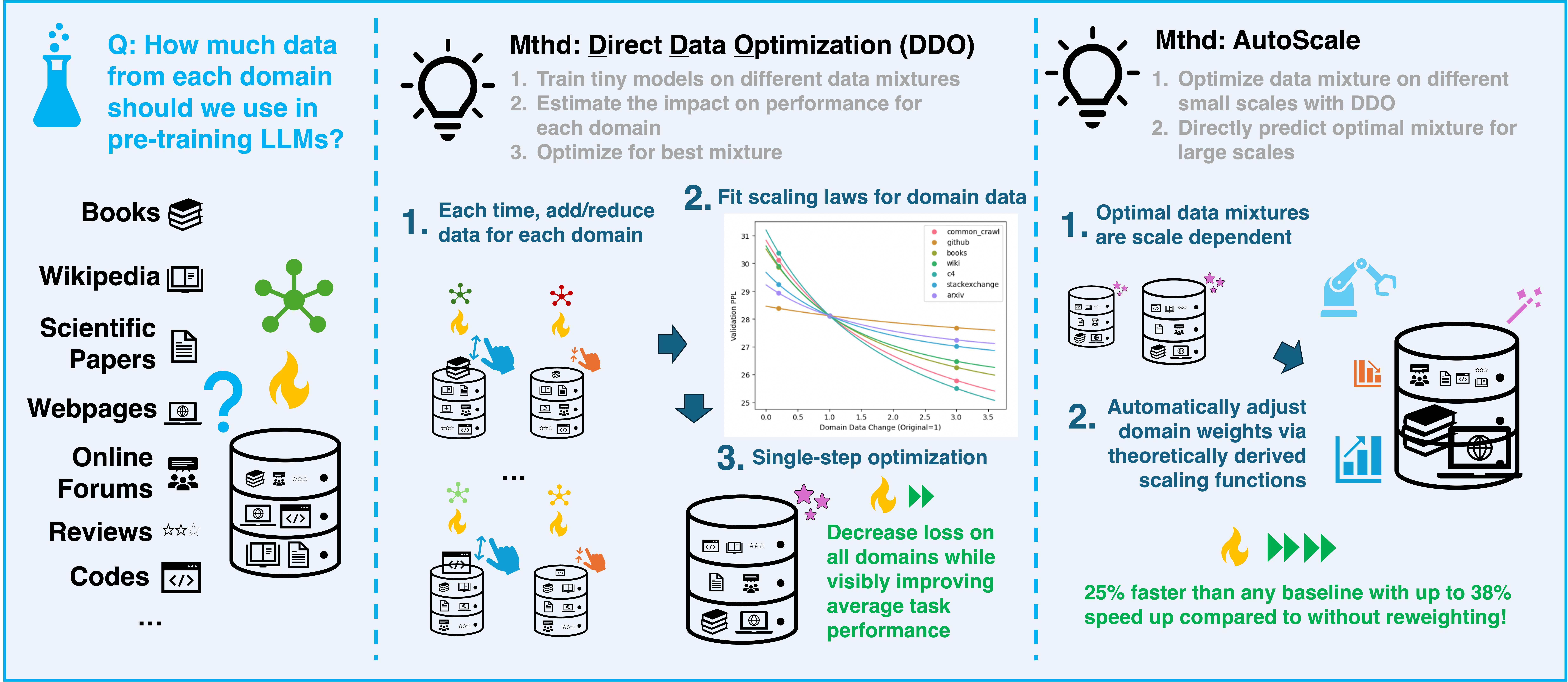
A majority of these works aim to first optimize data composition for a smaller proxy model and at a smaller data scale ([1, 5, 6]). Yet, this optimization is often conducted with alternative objectives not always aligned with the original objectives of minimizing evaluation loss. DoReMi [1] first trains a small reference model, and then trains a second proxy model with GroupDRO [7] to minimize the excessive domain loss relative to the reference model, where the domain weights of the proxy model will be the output. DOGE [5] trains a proxy model while tracking the first-order gradient of the model on evaluation domains (i.e., data influence) and optimizes domain weights based on the gradients, relying on infinitesimal approximations which may or may not be accurate for models trained with a practical learning rate. Data Mixing Laws [6] trains a number of proxy models to run a coarse grid search on the space of data mixtures and interpolate their performance with exponential functions to find the minimum. These methods often rely on ad-hoc hyperparameter tuning via trial and error. Further, the optimized weights are directly applied to training the target model on magnitudes of larger data scales. This implicitly poses a strong assumption that the "optimal data composition" is invariant of model sizes or data scales. Yet, optimal data composition is likely to shift with data size. Optimal curation at a smaller scale may not remain optimal at the target scale [8]. We refer to [9] and Appendix A for related works.

(a) Validation Perplexity. ($\downarrow$ lower is better)

(b) Downstream Task Performance at 96k Steps. ($\uparrow$ higher is better)

Figure 2: Training 774M Decoder-only LMs for 10B tokens (96k steps). AutoScale-predicted domain weights decrease validation PPL at least $28\%$ faster than any baseline with up to $38\%$ speed up. LLaMA weights yield a much better training efficiency than uniform weights when scaling up.

Given the challenges of optimizing data composition, an increasingly popular practice is to directly use domain weights that were designed for training previous models (e.g., LLaMA weights [10], The Pile weights [11]). For instance, [12] recently trained a 1B-parameter model on a combination of The Pile dataset, LLaMa (RedPajama [13]) training dataset, and Dolma [4] training dataset. However, these weights are optimized for specific applications that may be vastly different from the target scenario (e.g., model architecture, language modeling objectives, training data scale, etc.). Industry practice still relies on heuristics for mixing domain data [14, 12, 15]. Thus, the potential for improved training efficiency via principled domain reweighting remains unknown.

In this work, we propose a generic domain reweighting methodology for LLM pre-training to overcome these limitations. Our efforts are two-fold:

• First, we formalize the problem of finding compute-optimal data composition with domain reweighting as bi-level optimization. This allows for directly optimizing the final objective over data composition, circumventing most of the risks from heuristic designs. Further, we propose a practical solution algorithm, Direct Data Optimization (DDO), for determining a compute-optimal training data composition for a given data scale by estimating and optimizing over the neural scaling law of the data sources. This provides a global approximation to this problem, which allows finding the global optimum in a single step with high precision, achieving consistent results and reliable performance improvements robust to different use cases (Figure 4).

• Second, seminal work [16] suggests the possibility of attaining beyond-neural scaling law performance if one could find the best training dataset for each training data scale. We observe a similar pattern in optimizing training data composition for LLMs (Figure 3). We show that the shift in the optimal data composition with the scale of training complies with a simple function form and is empirically predictable. By fitting this pattern of shift at smaller scales, we are able to predict optimal data compositions at larger scales, automatically adjusting data composition for any training data scale and achieving beyond-neural scaling performance improvements on the target model. Correspondingly, we propose AutoScale, an automated tool that finds a compute-optimal data composition for training an LLM at the target scale. With optimal data compositions found at smaller scales, we fit the AutoScale predictor designed based on theoretical analysis with scaling laws and use it to determine optimal data composition at larger scales. Since one only needs to train models on small data scales where re-training is affordable, AutoScale does not require using proxy models with a smaller parameter size, avoiding the transferability issue between domain weights optimized on different models.

(a) DDO-Optimized Domain Weights

(b) Optimal Weights are Scale-dependent

Figure 3: Optimizing domain weights with DDO algorithm for pre-training 774M Decoder-only LMs (GPT-2 Large). Optimal domain weights are dependent on the scale of training data. A consistent shift can be observed. Using domain weights optimized for a different scale yields sub-optimal results, failing to fully realize the benefits of domain reweighting.

(a) Validation Loss ($\downarrow$ lower is better)

(b) Task Performance ($\uparrow$ higher is better)

Figure 4: Optimizing domain weights with DDO algorithm for pre-training Encoder-only LMs (BERT). DDO substantially reduces validation loss. After reweighting, all training domains’ loss has either decreased or remained unchanged. Out-of-domain loss on non-training domains has also decreased considerably. Enhanced performance has been observed on all GLUE tasks and SQuAD.

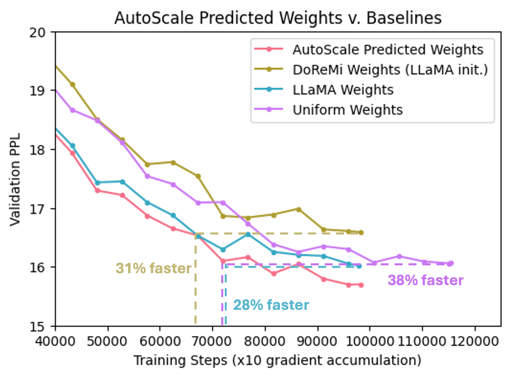
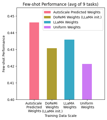
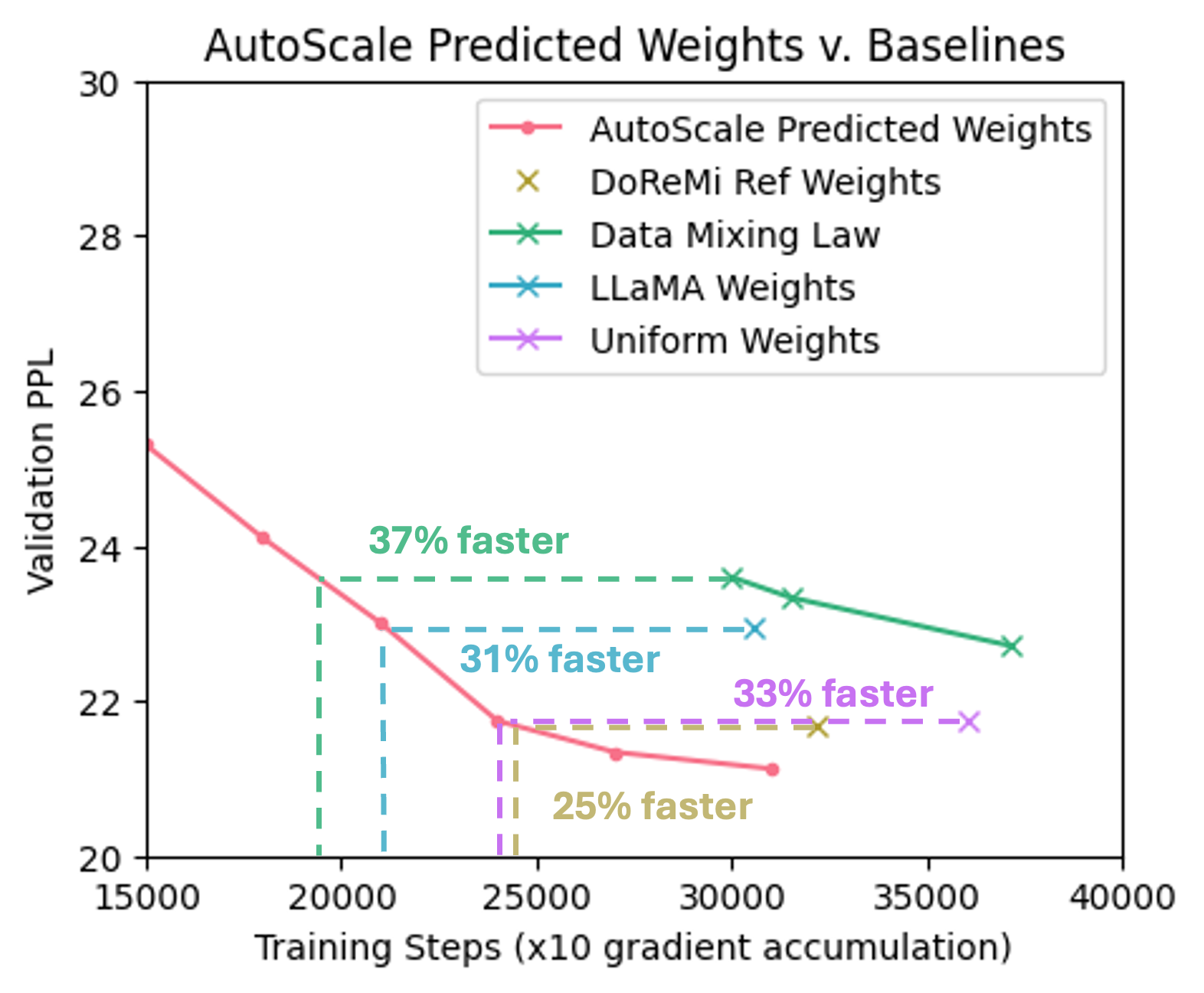
In empirical studies with pre-training 774M Decoder-only LMs (GPT-2 Large[17]) on RedPajama dataset, AutoScale decreases validation perplexity at least 25% faster than any baseline with up to 38% speed up compared to without reweighting, achieving the best overall performance over downstream tasks. On pre-training Encoder-only LMs (BERT [18]) with masked language modeling (MLM), compared to without reweighting, DDO decreases loss on all domains while visibly improving average task performance on GLUE benchmark [19] by 8.7% and on large-scale QA dataset, SQuAD [20], by 5.9%, where AutoScale further speeds up training by up to 28%. We found data sources with standard format such as Wikipedia and scientific papers, regarded as high quality, are most beneficial at smaller scales but observe sharp diminishing returns as the training data scales up. With more compute, data sources with diverse examples, such as CommonCrawl, demonstrate continued reductions in training loss even at considerably large training data scales.

2 Compute-optimal Training Data Compositions

Consider training an LLM on a data composition from multiple sources/domains. Proportions of data for each domain are referred to as “domain weights”. The goal is to find an optimal training data composition such that, for a given compute budget (i.e., training data size), the reduction in evaluation loss is maximized. For language models, the most commonly used evaluation metric is perplexity (PPL), defined as the exponentiation of cross-entropy loss. In information theory, reduction in perplexity is considered to measure the amount of information gain. Thus, the objective is to maximize training efficiency by finding "compute-optimal" domain weights for the training data. This setup has been adopted in this line of research [1, 3, 5] and we will also follow in this work. We first formulate this as a bi-level optimization problem and then introduce an efficient solution approach to solve it.

2.1 Problem Formulation

Consider training an LLM on a data composition $S$ from $m$ domains, $D_{1},D_{2},\cdots,D_{m}$. Let $S=\{S_{1},S_{2},\cdots,S_{m}\}$ denote the training dataset where $S_{i}$ is the subset of training data from each domain. The domain weights $\mathbf{w}=[w_{1},w_{2},\cdots,w_{m}]^{T}$ are defined as the proportions of data for each domain. Namely, letting $N=|S|$ denote the amount of total tokens of training data, domain weights are given as $w_{i}=N_{i}/N$, where $|S_{i}|$ denotes the amount of tokens for training subset $S_{i}$. Let $S(N,\mathbf{w})$ denote the dataset of $N$ tokens composed from different domains using the weights $\mathbf{w}$. Let $\mathcal{A}(S)$ denote a learning algorithm (i.e., the model) parameterized by $\theta$ trained on data $S$ with empirical risk minimization (ERM), given as $\mathcal{A}(S):={\arg\min}_{\theta}\mathcal{L}(\theta,S)$ where $\mathcal{L}(\cdot,\cdot)$ denotes the loss function used in training. With slight abuse of notation, we use $\mathcal{A}(N,\mathbf{w})$ as shorthand for $\mathcal{A}(S(N,\mathbf{w}))$. We would like to maximize the amount of information gain and achieve maximum loss reduction during training, given as $\min_{\mathbf{w}\in\mathbb{W}^{m}}\mathcal{L}^{P}_{v}(\mathcal{A}(N,\mathbf{w}))=\sum_{i=1}^{m}\mathcal{L}^{P}_{i}(\mathbf{\mathcal{A}}(N,\mathbf{w}),D_{i}^{v})$, where $\mathcal{L}^{P}_{v}(\cdot)$ and $\mathcal{L}^{P}_{i}(\cdot)$ denote total evaluation loss and the loss of the model evaluated on the validation data of individual domains, respectively; the space of weights $\mathbb{W}^{m}$ is the hyperplane of the probability simplex $\mathbb{W}^{m}=\{\mathbf{w}|w_{1}+w_{2}+\cdots+w_{m}=1\}\cap\{\mathbf{w}|0\leq w_{i}\leq 1,\forall i\in\{1,2,\cdots,m\}\}$. Then, the optimal domain weights, $\mathbf{w^{*}}$, are given as the minimizer of the objective,

$$\mathbf{w^{*}}=\arg\min_{\mathbf{w}\in\mathbb{W}^{m}}\frac{1}{m}\sum_{i=1}^{m}\mathcal{L}^{P}_{i}(\mathbf{\mathcal{A}}(N,\mathbf{w)},D_{i}^{v})\quad\text{s.t.}\,\,\,\,\mathcal{A}(N,\mathbf{w})=\arg\min_{\theta}\mathcal{L}(\theta,S(N,\mathbf{w}))\vspace{-1em}$$ (1)

where perplexity is adopted as the loss metric. This formulation naturally produces a bi-level optimization problem, where the upper-level problem (left) seeks the optimal domain weights, while the lower-level problem (right) is training the model with ERM on the data defined by certain weights. A general approach is to solve it with gradient descent, $\mathbf{w}^{t+1}=\mathbf{w}^{t}-\eta\cdot\frac{\partial\mathcal{L}^{P}_{v}(\mathcal{A}(N,\mathbf{w}^{t}))}{\partial\mathbf{w}}$. Since there is no tractable form of analytical expression for $\mathcal{A}$, this gradient needs to be estimated with empirical methods (e.g., approximated by finite difference), requiring repetitive re-training of the model at each update. It is worth noting that despite the rich literature on bi-level optimization [21], traditional methods either rely on differentiating through the optimization process involved in the lower-level problem or require solving a linear system, which are not scalable for the setting of our interest.

2.2 A Practical Solution via Scaling-law-inspired Approximation

Re-training LLMs is usually prohibitively expensive. The standard practice is to optimize the data composition with proxy models where re-training is plausible, and then optimized domain weights are used to train models at full scale [1, 5, 6]. The proxy model often has a similar architecture to the target model but is smaller in parameter size and/or trained with much less data. The assumption is the performance achieved on the proxy model could provide an effective indicator for performance on the target model. Even for proxy models, solving this bi-level optimization problem via gradient methods can still be expensive, which necessitates a trade-off between algorithmic efficiency and solution quality. Current work [1, 5, 6] mostly employs heuristic methods to conduct this optimization and achieves varying results, rendering the users hard to tell when they will work or fail. Instead, we provide a global approximation to this problem, which allows finding the global optimum in a single step with high precision. This enables achieving consistent results and reliable performance improvements robust to different use cases.

Neural scaling laws suggest the relationship between a model’s evaluation loss and the size of its training data can be well-represented by power law functions [22] $\mathcal{L}^{P}_{v}(\mathcal{A}(N,\mathbf{w}))=N^{-\gamma}+\mathcal{L}_{0}$ where constants $\mathcal{L}_{0}$ denotes some irreducible loss and $\gamma\geq 0$ is some scaling coefficient. Drawing inspirations from [23], we propose the following approximation. Consider a model trained on data with size $N$ and domain weights $\mathbf{w}$. If the amount of training data from one domain $D_{i}$ is changed from $N_{i}$ to $N_{i}^{\prime}$ with the amount of training from other domains unchanged, we approximate the new model’s evaluation loss after re-training with a power law function of $N_{i}^{\prime}$:

$$\mathcal{L}^{P}_{v}(\mathcal{A}(N^{\prime},\mathbf{w^{\prime}}))=(N_{0}^{i}+N_{i}^{\prime})^{-b_{i}}+c_{i},$$ (2)

where $b_{i},c_{i}$ are constants associated with domain $i$, $N^{\prime}=N+(N_{i}^{\prime}-N_{i})$ denotes the updated amount of training data, and $w_{i}^{\prime}=N_{i}^{\prime}/N^{\prime}$ denotes the updated domain weights. $N_{0}^{i}$ estimates the evaluation loss when the amount of training data from domain $i$ is zero (i.e., $N_{i}^{\prime}=0$) and effectively measures the effect of data from all other domains. From this regard, $N_{0}^{i}$ can be interpreted as the equivalent data size for training data from domains other than $i$. Notably, this formulation aligns with empirical findings in the prior literature [23, 6].

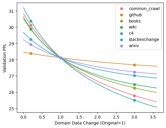
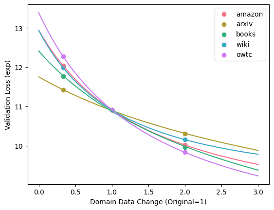
We propose the following procedure to fit the parameters in (2). We re-train two models with different $N_{i}^{\prime}$ and $N_{i}^{\prime\prime}$ and calculate their evaluation loss. Then, together with evaluation loss for the original model trained with $N_{i}$, the parameters $b_{i}$, $c_{i}$ and $N_{0}^{i}$ can be estimated via ordinary least square (OLS) fitting. The difference in evaluation loss compared to the original model is given as $\mathcal{L}^{P}_{v}(\mathcal{A}(N^{\prime},\mathbf{w^{\prime}}))-\mathcal{L}^{P}_{v}(\mathcal{A}(N,\mathbf{w}))=(N_{0}^{i}+N_{i}^{\prime})^{-b_{i}}-(N_{0}^{i}+N_{i})^{-b_{i}}.$ Repeating this process and fitting the scaling functions for each domain, finally, we express the evaluation loss as a function of the amount of data from each domain as their summation: $\mathcal{L}^{P}_{v}(\mathcal{A}(N^{\prime},\mathbf{w^{\prime}}))-\mathcal{L}^{P}_{v}(\mathcal{A}(N,\mathbf{w}))=\sum_{i=1}^{m}\left[(N_{0}^{i}+N_{i}^{\prime})^{-b_{i}}-(N_{0}^{i}+N_{i})^{-b_{i}}\right]$ where $N^{\prime}=N+\sum_{i}(N_{i}^{\prime}-N_{i})$ and $w_{i}^{\prime}=N_{i}^{\prime}/N^{\prime}$. Empirically, evaluation loss is shown to be well represented by such function form (Figure 5). This representation lends us an analytical form for the objective of the problem, which becomes

$$\mathbf{w^{*}}=\arg\min_{\mathbf{w^{\prime}}\in\mathbb{W}^{m}}\sum_{i=1}^{m}\left[(N_{0}^{i}+N_{i}^{\prime})^{-b_{i}}-(N_{0}^{i}+N_{i})^{-b_{i}}\right]=\arg\min_{\mathbf{w^{\prime}}\in\mathbb{W}^{m}}\sum_{i=1}^{m}(N_{0}^{i}+w_{i}^{\prime}\cdot N)^{-b_{i}}.$$

To derive the final objective from the middle one, we first note that $(N_{0}^{i}+N_{i})^{-b_{i}}$ is independent of $\mathbf{w}^{\prime}$. Moreover, when we retrain model on the perturbed data sizes $N_{i}^{\prime}$, we explicitly constrain the total amount of training data to be the same as before, i.e., $\sum_{i}N_{i}^{\prime}=N$. Hence, $(N_{0}^{i}+N_{i}^{\prime})^{-b_{i}}=(N_{0}^{i}+w_{i}^{\prime}\cdot N^{\prime})^{-b_{i}}=(N_{0}^{i}+w_{i}^{\prime}\cdot N)^{-b_{i}}$. Since the objective is defined as the summation of convex functions, we end up with a convex optimization problem. With the constraint on the probability simplex and the objective being easily differentiable, the problem can be solved extremely efficiently using projected gradient descent [24]. We term this solution approach as DDO Algorithm (Direct Data Optimization). We provide its pseudocode below and an operational pipeline in Appendix B.

Algorithm 1 Direct Data Optimization (DDO)

$m$ domains (data sources) with data $D_{1}\dots D_{m}$, data budget $N_{0}$ ($\ll$ data budget for full-scale training), training dataset $S$, model $\mathcal{A}$, validation loss function $\mathcal{L}_{v}$.

Initialize weights for all domains $\forall i\in\{1,\dots m\}$: $w_{i}\leftarrow 1/m$;

Initialize training data for all domains $\forall i\in\{1,\dots m\}$: sample $S_{i}\subset D_{i}$ where $|S_{i}|=w_{i}\cdot N$;

Train the model on data $S=\{S_{1}\dots S_{m}\}$ and evaluates its loss $\mathcal{L}_{0}\leftarrow\mathcal{L}_{v}(\mathcal{A}(S))$;

for $j$ from $1$ to $m$ do

     $w_{j}^{+}\leftarrow 3\cdot w_{j}$; $\triangleright$ Perturb domain weights (+)

     Resample $S_{j}^{+}\subset D_{j}$ where $|S_{j}^{+}|=w_{j}^{+}\cdot N$;

     Train the model on data $S=(\{S_{1}\dots S_{m}\}\setminus S_{i})\cup S_{j}^{+}$ and evaluates its loss $\mathcal{L}_{j}^{+}\leftarrow\mathcal{L}_{v}(\mathcal{A}(S))$;

     $w_{j}^{-}\leftarrow\frac{1}{3}\cdot w_{j}$; $\triangleright$ Perturb domain weights (-, optional)

     Resample $S_{j}^{-}\subset D_{j}$ where $|S_{j}^{-}|=w_{j}^{-}\cdot N$;

     Train the model on data $S=(\{S_{1}\dots S_{m}\}\setminus S_{i})\cup S_{j}^{-}$ and evaluates its loss $\mathcal{L}_{j}^{-}\leftarrow\mathcal{L}_{v}(\mathcal{A}(S))$;

     OLS fit for scaling functions $b_{j},c_{j}=\arg\min_{b_{j},c_{j}}[\mathcal{L}_{0}-(w_{i}\cdot N)^{-b_{j}}-c_{j}]^{2}+[\mathcal{L}_{j}^{+}-(3\cdot w_{i}\cdot N)^{-b_{j}}-c_{j}]^{2}+[\mathcal{L}_{j}^{-}-(\frac{1}{3}\cdot w_{i}\cdot N)^{-b_{j}}-c_{j}]^{2}$;

end for

Output optimized domain weights $\mathbf{w^{*}}=\arg\min_{\mathbf{w^{\prime}}\in\mathbb{W}^{m}}\sum_{i=1}^{m}(w_{i}^{\prime}\cdot N)^{-b_{i}}$.

(a) 774M Decoder-only LMs (GPT-2 Large)

(b) Encoder-only LMs (BERT-case)

Figure 5: Fitting validation loss with power-law functions, directly approximating how loss changes with each domain’s data quantity. Compared to BERT models trained with MLM (right), GPT models trained with CLM (left) demonstrate a much stronger response to domain reweighting. In final results, GPT/CLM achieved >2x speed-up margins relative to uniform weights compared to BERT/MLM.

3 Predicting Optimal Data Compositions for Larger Scales

While Section 2 provides an algorithmic framework to optimize the data composition at any scale, it is computationally expensive to directly perform optimization at a large target scale because it requires retraining models, which is only practical at a smaller scale. This section will investigate how to predict the optimal composition at a larger scale based on the composition optimized at smaller scales. In particular, we show that the optimal composition follows an exponential trend with respect to the scale, derived through a novel theoretical analysis and further justified through empirical observations.

3.1 Scaling Domain Weights

Recall that neural scaling laws give the relationship between evaluation loss and training data quantity as $\mathcal{L}=N^{-\gamma}+\mathcal{L}_{0}$ where $\mathcal{L}$ is the evaluation loss (e.g., perplexity), $\mathcal{L}_{0}$ denotes some irreducible loss, and $\gamma\geq 0$ are some constant. $(\mathcal{L}_{0},\gamma)$ can be fitted empirically. Consider a stylized case where the evaluation metric is aggregated loss over multiple independent tasks where each training sample will only contribute to a single task and the loss of each task only scales with the amount of training data contributing to this task as a power law function. Then, for a total of $m$ tasks, the aggregated evaluation loss scales as the following $\mathcal{L}=\mathcal{L}_{0}+\sum_{i=1}^{m}\beta_{i}\cdot N_{i}^{-\gamma_{i}}$, where $\mathcal{L}_{0}$ denotes some irreducible loss, $N_{i}$ denotes the amount of data contributing to task $i$, and constants $\beta_{i}\geq 0$ and $\gamma_{i}\geq 0$ are coefficients associated with task $i$. Define diagonal matrix $\mathbf{N}=diag\{N_{1},N_{2},\cdots N_{m}\}$. For a training data scale $N=\sum_{i}N_{i}$, define compute-optimal data composition $\mathbf{N}=diag\{N_{1}^{*},N_{2}^{*},\cdots N_{m}^{*}\}$ as the minimizer of $\mathcal{L}$, given as $\mathbf{N^{*}}={\arg\min}_{\sum_{i}N_{i}=N}\mathcal{L}_{0}+\sum_{i=1}^{m}\beta_{i}\cdot N_{i}^{-\gamma_{i}}$. We propose the following theorem, which states the optimal data composition scales in exponential-style functions with the amount of training data and can be directly predictable from that of smaller scales.

Theorem 1 (Scaling Law for Optimal Data Compositions).

For an evaluation loss that is aggregated over multiple independent tasks as described above. If we have optimal data compositions $\mathbf{N^{(1)*}}=diag\{N_{1}^{(1)*},N_{2}^{(1)*},\cdots N_{m}^{(1)*}\}$ which minimizes $\mathcal{L}$ s.t. $\sum_{i}N_{i}^{(1)*}=N^{(1)}$ and $\mathbf{N^{(2)*}}=diag\{N_{1}^{(2)*},N_{2}^{(2)*},\cdots N_{m}^{(2)*}\}$ minimizes $\mathcal{L}$ s.t. $\sum_{i}N_{i}^{(2)*}=N^{(2)}$ where $N^{(1)}\neq N^{(2)}$, then, optimal data compositions at other data scales $\mathbf{N^{(3)*}}=diag\{N_{1}^{(3)*},N_{2}^{(3)*},\cdots N_{m}^{(3)*}\}$ which minimizes $\mathcal{L}$ s.t. $\sum_{i}N_{i}^{(3)*}=N^{(3)}$ where $N^{(3)}\neq N^{(2)}\neq N^{(1)}$ can be given as $\mathbf{N^{(3)*}}=\mathbf{N^{(2)*}}(\mathbf{N^{(1)*}})^{-1}\mathbf{N^{(2)*}}$.

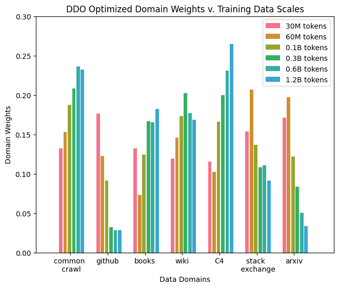
See Appendix C.1 for the formal theorem statement and a complete proof, which is based on the optimality condition for convex optimization. At an optimal data composition, KKT condition [24] gives that we have the partial derivative of the loss function w.r.t. the amount of data from each domain equal to each other. This holds for any data scale $N$. The power law scaling function for the loss yields an exponential-style scaling function for the optimal data quantity of each task. Examples for illustration are also provided in C.1. We built our theory from a stylized example which assumes the evaluation metric is composed of independent tasks with separate scaling laws. In Appendix C.2, we further extend this theory to a general case where the same conclusion can be reached without the independence assumption, where we consider the evaluation to be composed of a number of indepedent sub-tasks ("latent skills" [25]) which are hidden variables. Finally, we note that empirical results are shown to be highly consistent with the derivations above. In Figure 3(a), we observe a consistent shifting pattern for optimal data composition with the scale of training data, which can be well-described by the function forms described above.

3.2 AutoScale: Automatic Prediction of Optimal Training Data at Larger Scales

We conclude the section by presenting a novel tool–AutoScale, which automatically predicts optimal training data compositions at larger scales.

Algorithm 2 AutoScale

Optimal domain weights (obtained from DDO) $\mathbf{w^{(1)*}}$at data scale $N^{(1)}$ and $\mathbf{w^{(2)*}}$ at data scale $N^{(2)}$, target data scale $N^{(t)}$, where $N^{(1)}<N^{(2)}<N^{(t)}$.

Optimal domain data $\mathbf{N^{(1)*}}\leftarrow\mathbf{w^{(1)*}}\cdot N^{(1)}$;

Optimal domain data $\mathbf{N^{(2)*}}\leftarrow\mathbf{w^{(2)*}}\cdot N^{(2)}$;

Next optimal domain data $\mathbf{N^{(x)*}}\leftarrow\mathbf{N^{(2)*}}(\mathbf{N^{(1)*}})^{-1}\mathbf{N^{(2)*}}$;

Next data scale $N^{(x)}\leftarrow\sum_{i}N_{i}^{(x)*}$;

while $N^{(x)}<N^{(t)}$ do

     Next optimal domain data $\mathbf{N^{(x)*}}\leftarrow\mathbf{N^{(x)*}}(\mathbf{N^{(1)*}})^{-1}\mathbf{N^{(2)*}}$;

     Next data scale $N^{(x)}\leftarrow\sum_{i}N_{i}^{(x)*}$;

end while

Output predicted optimal domain weights $\mathbf{w^{(t)*}}\leftarrow\mathbf{N^{(x)*}}/N^{(x)}$.

Theoretical analysis above shows that the optimal quantity for each domain scales in exponential-style functions with training data size. We leverage this result to enable the automatic prediction of optimal training data compositions at larger scales from optimal compositions at small scales. First, for two smaller training data scales $N^{(1)}$ and $N^{(2)}$ where $N^{(1)}\neq N^{(2)}$, find their optimal training data compositions $\mathbf{N^{(1)*}}$ and $\mathbf{N^{(2)}*}$ where $\sum_{i}N_{i}^{(1)*}=^{(1)}$ and $\sum_{i}N_{i}^{(2)*}=N^{(2)}$ using DDO algorithm provided in Section 2. Models trained at scales $N$ and $N^{\prime}$ are considered proxy models where re-training these models is affordable. Since $N^{(1)}$ and $N^{(2)}$ are small data scales where re-training these models is affordable, AutoScale does not require using proxy models with a smaller parameter size, avoiding the transferability issue between domain weights optimized on different models. Then, $\mathbf{N^{(1)*}}$ and $\mathbf{N^{(2)*}}$ yield the optimal training data composition at the next scale as $\mathbf{N^{(3)*}}=\mathbf{N^{(2)*}}(\mathbf{N^{(1)*}})^{-1}\mathbf{N^{(2)*}}$, where $N_{i}^{(3)*}=(N_{i}^{(2)*})^{2}/N_{i}^{(1)*}$ is the optimal amount of training data for each domain. This gives that for data scale $N^{(3)}=\sum_{i}N_{i}^{(3)*}$, optimal domain weights are given as $w_{i}^{(3)*}=N_{i}^{(3)*}/N^{(3)}$. Then, $\mathbf{N^{(3)*}}$ can be combined with either $\mathbf{N^{(1)*}}$ or $\mathbf{N^{(2)*}}$ to make the next prediction. Repeat this process until the target training data scale is reached. The procedure is described in the pseudocode above. Operational pipeline is provided in Appendix B.

4 Empirical Results

We showcase our proposed algorithms in two sets of empirical studies: Causal Language Modeling (CLM) in Section 4.2, and Masked Language Modeling (MLM) in Section 4.3. We train models with up to 10B tokens and report the number of steps saved to reach the same evaluation loss (perplexity). We also report downstream task performance to benchmark performance improvements after training the same number of steps.

4.1 Experimental setup

In Section 4.2, we pretrain 774M Decoder-only LMs (GPT-2 Large architecture [17]) from scratch on the RedPajama dataset [13]. RedPajama dataset is an open-source reproduction of the training data used for LLaMA-1/2 models [10], totaling 1.2T tokens from 7 data domains with proportions: Common Crawl (67%), C4 [26] (15%), GitHub (4.5%), Wikipedia (4.5%), ArXiv (2.5%), and StackExchange (2.0%). In Section 4.3, we pretrain 110M Encoder-only LMs (BERT-base architecture [27]) from scratch on data from 5 typical sources—Amazon Reviews, Arxiv, Books, Wikipedia, and Open WebText Corpus [28]. Further details are in Appendix D.1 and D.2. Runtime and GPU hours are documented in Appendix D.7.

4.2 Causal Language Modeling with Decoder-only LMs (GPT)

Baselines

In total, we report results for our methods (DDO and AutoScale) and 5 baselines–Uniform, LLaMA weights (curated), DoReMi (LLaMA weights initialization), Data Mixing Laws from [6] and DoReMi from [1] (uniform initialization). Uniform weights uniformly sample data from all domains, resulting in the same number of training tokens from each domain. LLaMA weights are a set of curated domain weights heuristically tuned for training LLaMA-1/2 models. We implemented DoReMi proposed in [1]. DoReMi trains two smaller-scale auxiliary models (proxy models). First, a reference model is trained with the dataset’s original domain weights, which are the LLaMA weights for RedPajama dataset. Then, optimized domain weights are obtained by using a proxy model to minimize the worst-case excess loss across different domains. We train both auxiliary models for 50K steps. Implementation details are available in Appendix D.3. Besides, we compare with 2 domain weights from existing literature, which are optimized on the same data domains RedPajama dataset with similar Decoder-only LMs. Data Mixing Laws [6] first performs a grid search on the space of possible data mixtures and records evaluation loss for proxy models trained on these mixtures. Then, the loss is interpolated with exponential functions to find the optimal domain weights for the proxy model. DOGE [5] also implements DoReMi [1] with auxiliary models trained for 50K steps but with the reference model trained with uniform weights. We evaluate the model trained on these domain weights to present a complete landscape.

Evaluation We test the perplexity on the held-out dataset, comprising 10K samples each from the 7 domains. For downstream tasks, we include: BoolQ [29] (zero-shot), HellaSwag [30] (zero-shot, 10-shot), PIQA [31] (zero-shot), TruthfulQA [32] (zero-shot), PubMedQA [33] (10-shot), CrowsPairs [34] (25-shot), and ARC-Easy [35] (zero-shot). Additionally, BBH Novel Concepts [36] task is added to the aggregated results for models trained beyond 10B tokens, making a total of 9 tasks. We select tasks that ensure the model’s performance surpasses random guessing, spanning from question answering and commonsense inference to bias identification and scientific problem solving. These tasks provide a comprehensive assessment of model performance [12, 37]. We adopt the evaluation framework from [38]. More details on downstream datasets are available in Appendix D.4.

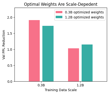
Direct Data Optimization (DDO): We conduct DDO Algorithm to optimize domain weights for proxy models (774M Decoder-only LMs) trained from scratch with 30M to 1.2B tokens. Takeaway 1a:, as depicted in Figure 3(a), optimal domain weights for each training data scale are visibly different and demonstrate a clear shifting pattern. We found data sources with standard format such as Wikipedia and scientific papers, regarded as high quality, are most beneficial at smaller scales and observe sharp diminishing returns as the training data scales up. With more compute, data sources with diverse examples, such as CommonCrawl, continue to reduce training loss even at considerably large training data scales. We validated this observation in Figure 3(b), where we trained two models with 0.3B tokens with domain weights optimized at 0.3B tokens and 1.2B tokens, and two models with 1.2B tokens with these weights, respectively. Takeaway 1b: the results show that, the optimal weights on only optimal at the scale it is optimized and become suboptimal when applied on other scales.

Predicting Optimal Weights at Larger Scales with AutoScale: With DDO-optimized weights from proxy models trained up to 0.6B tokens, we fit AutoScale predictor and use it to visualize how the optimal domain weights will shift as we continue scaling up training data. As depicted in Figure 6, as the training data scale grows, data sources with diverse examples, such as C4 and CommonCrawl, will take up a considerable proportion of training data. Takeaway 2a: therefore, we expect LLaMA weights will perform better when the training data scale is sufficiently large. The results also suggest training on data from Books domain will continue to provide benefits. Takeaway 2b: thus, AutoScale-predicted domain weights give a larger weight to Books domain compared to baselines which counterintuitively downweight high-quality book contents.

(a) AutoScale-predicted optimal data quantity for each domain as training data scales up.

(b) AutoScale-predicted optimal domain weights as training data scales up.

Figure 6: AutoScale-predicted domain weights for training 774M Decoder-only LMs. Optimal data quantity for each domain grows in exponential-style functions with training data scale (left) where data sources with diverse samples (e.g., C4) are unweighted relative to domains with standard format (e.g., Wikipedia).

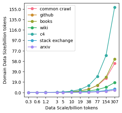
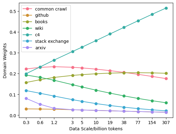
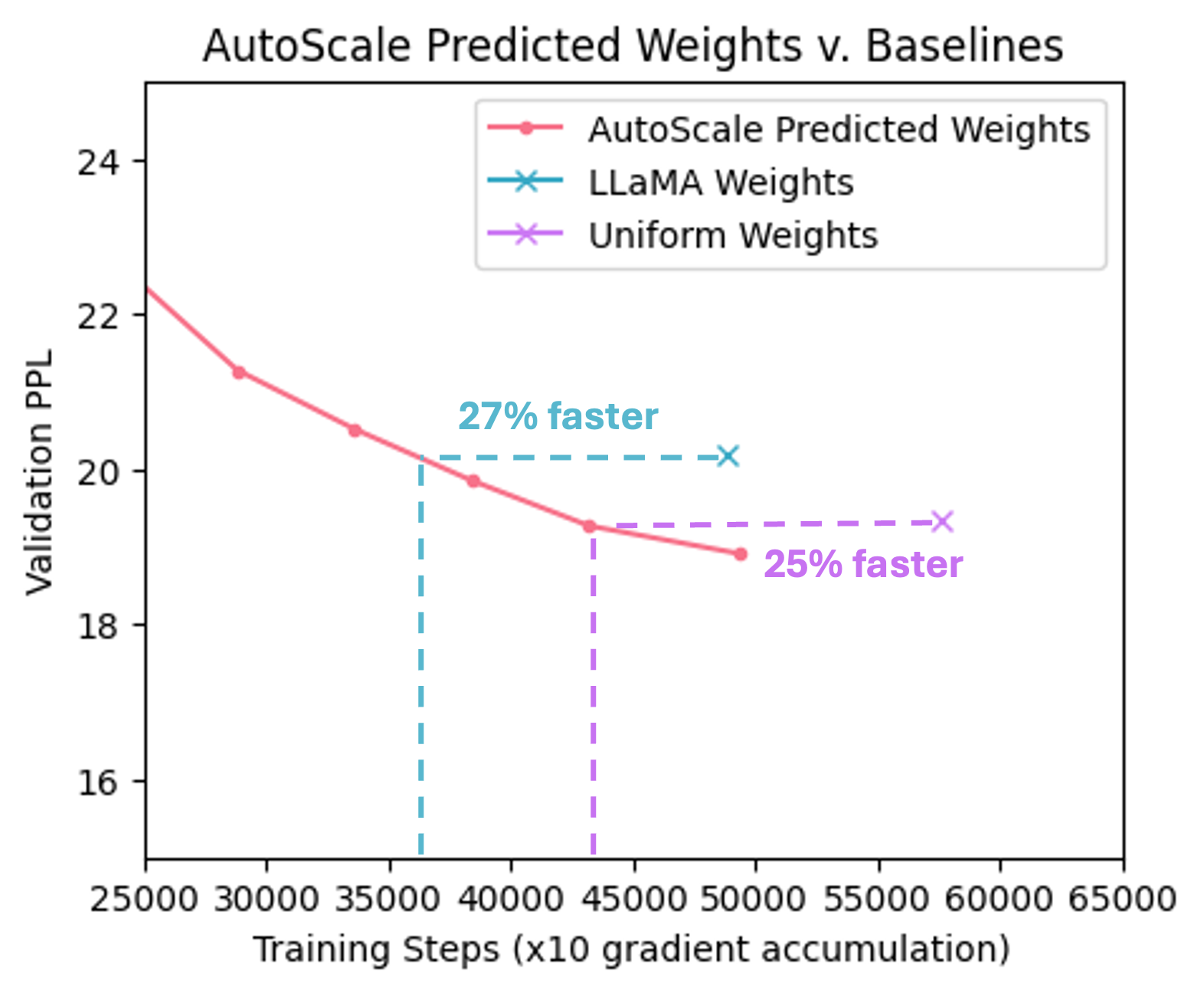
Subsequently, to examine AutoScale-predicted weights, we train models on larger scales with 3B, 5B, and 10B tokens. On 3B training data, we compare AutoScale-predicted weights with Uniform weights, LLaMA weights, DoReMi weights from [5] (uniform initialization), and Data Mixing Laws weights from [6]. Takeaway 2c: in both 3B and 5B results (Figure 8), AutoScale achieves the lowest validation perplexity after the same steps, at least $25\%$ faster than any baseline with up to $37\%$ speed up. Provided in Table 7, AutoScale-predicted weights significantly reduced the loss on Books domain and also achieved much lowered worst-domain perplexity. When testing the few-shot performance on 8 downstream tasks, the model trained with AutoScale-predicted weights achieves the best overall performance, as shown in Table 1. Results for models trained with 10B tokens are depicted in Figure 2, where we added the comparison with DoReMi initialized with LLaMA weights. AutoScale-predicted weights consistently outperform any baseline with a $28\%$ to $38\%$ margin and demonstrate advantageous performance on downstream tasks. Takeaway 2d: echoing our predictions, as training data scales up, LLaMA weights visibly outperform uniform domain weights. For additional results see Appendix D.5.

Method/Task	truthfulqa	pubmedqa	piqa	hellaswag	crows_pairs	boolq	arc_easy	hellaswag	Avg
	_mc2			(10-shot)	_english			(zero-shot)
Uniform Weights	0.4526	0.438	0.6115	0.2923	0.5886	0.5636	0.3742	0.2907	0.4514
LLaMA Weights	0.434	0.492	0.6055	0.2944	0.5903	0.5612	0.3956	0.2952	0.4585
AutoScale (ours)	0.4385	0.536	0.6202	0.3021	0.585	0.6141	0.3977	0.303	0.4746
Data Mixing Laws (ref)	0.4537	0.468	0.6061	0.2951	0.5778	0.6162	0.3771	0.2938	0.4610

Table 1: Downstream task performance for 774M Decoder-only LMs trained for 3B tokens. Models trained with AutoScale-predicted weights achieve the best overall performance across the tasks.

4.3 Masked Language Modeling with Encoder-only LMs (BERT)

We examine the model’s MLM loss on held-out datasets, comprising 10K samples each from the 5 training domains. Additionally, as an auxiliary evaluation, we also test the MLM loss on 3 non-training held-out domains. To be consistent with the perplexity loss used in CLM, we report the exponential cross-entropy loss for MLM. We evaluate the model’s task performance on GLUE benchmark [19] (with 8 diverse tasks for natural language understanding (NLU)) and SQuAD [20] (a large-scale QA dataset). Evaluation details can be found in Appendix D.4. We examine the uniform weights as the baseline.

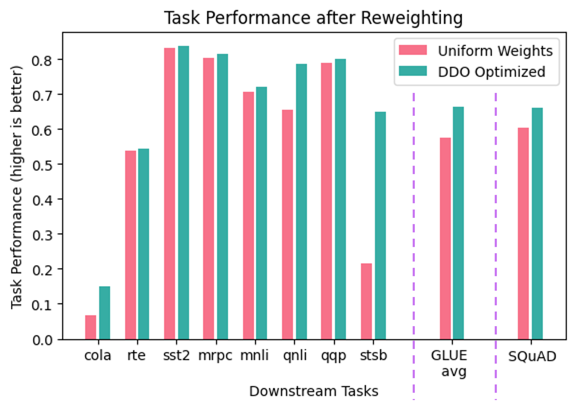
Direct Data Optimization (DDO): We conduct DDO Algorithm to optimize domain weights for proxy models (110M Encoder-only LMs) trained from scratch with MLM on 1GB data. Results for DDO-optimized weights are shown in Figure 4. Takeaway 3a: DDO visibly decreased the model’s validation loss on all training domains as well as held-out non-training domains, demonstrating its effectiveness in improving training efficiency and model utility. Takeaway 3b: when testing on GLUE benchmark and SQuAD dataset, consistent with the reduced evaluation loss, DDO-optimized weights are shown to improve the model’s performance on downstream tasks by a notable margin.

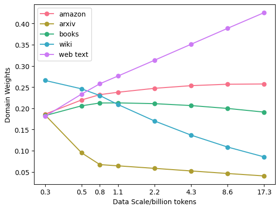
Predicting Optimal Weights at Larger Scales with AutoScale: With DDO-optimized weights from proxy models trained up to 0.5B tokens, we fit AutoScale predictor and use it to visualize how the optimal domain weights will shift as we continue scaling up training data. Takeaway 4a: as depicted in Figure 11, similar to the pattern described above, as the training data scale grows, data sources with diverse examples, such as WebText and Amazon Reviews, become increasingly important over standard domains, such as Wikipedia and Arxiv. One hypothesis is such data sources contain samples on diverse topics and language styles, providing rich information compared to domains with clean, standard text. We train models with MLM for up to 288k steps (which corresponds to 120% of the pertaining data size for BERT-base when first proposed in [18]). Takeaway 4b: table 2 shows that, compared to without reweighting (uniform weights), AutoScale-predicted weights speed up training by 16.7% on most data scales with an around 10% speedup on the largest scale, validating its consistent effectiveness. Takeaway 4c: nonetheless, the speedup is less impressive than in the results for Decoder-only LMs, demonstrating the different response to domain reweighting for models with different architecture or language modeling objectives. This is first hinted at in Figure 5, where the evaluation loss has a similar response to data from different domains, suggesting limited potential for performance improvements from domain reweighting.

Data Scale/steps	18k	36k	72k	144k	288k
Final Loss (exp)	38.32	16.94	10.97	8.13	6.30
Steps Saved	5k (28%)	5k (14%)	10k (14%)	20k (14%)	20k (10%)

Table 2: AutoScale notably improving training efficiency for BERT models on all scales–even for a considerably large scale, 288k steps, the speedup margin remains visible.

5 Conclusions

In this work, we demonstrate that the optimal data composition for a fixed compute budget varies depending on the scale of the training data, showcasing that the common practice of empirically determining an optimal composition using small-scale experiments will not yield the optimal data mixtures when scaling up to the final model. Addressing this challenge, we propose AutoScale, an automated tool that finds a compute-optimal data composition for training at any desired target scale. In empirical studies with pre-training 774M Decoder-only LMs and Ecoder-only LMs, AutoScale decreases validation perplexity at least 25% faster than any baseline with up to 38% speed up compared to without reweighting, achieving the best overall performance across downstream tasks.

Limitations and Future Work

The promising results achieved by AutoScale in optimizing data composition for large-scale language model pretraining open up some intriguing avenues for future exploration. (1) Generalizability: It will be interesting to extend this research to larger-scale settings, other data modalities, and more comprehensive evaluation benchmarks, and re-examine the validity of insights provided by the experiments at the scale that we work on. (2) Direct optimization of downstream performance: In practice, the capabilities of LLMs are characterized by their performance on various downstream tasks, and the perplexity loss that we focused on in this study is only a rough, inaccurate proxy for downstream performance. It will be interesting to extend AutoScale to directly optimize downstream performance. (3) More fine-grained data curation: AutoScale works with fixed data domains and only optimizes how the domains are mixed together, confining the optimization space. Intuitively, if one can strategically select the corpus within each domain and even adapt the data selection strategy to different stages of training, further improvements could be achieved.

Broader Impacts

Reducing the complexity and resource requirements associated with pretraining LLMs, AutoScale contributes to the democratization of AI. Smaller organizations, academic institutions, and individual researchers can more easily participate in cutting-edge AI research and development, fostering innovation and collaboration across the AI community. Moreover, learning from massive amounts of data requires large and costly computational resources, which not only consume substantial energy but also generate a significant carbon footprint, contributing to environmental issues. Furthermore, these resources quickly become obsolete due to the rapid pace of technological advancements, leading to e-waste. This research makes contributions to mitigating these issues by improving the efficiency of resource utilization in AI training.

[sections] [sections]l1

Appendix A Extended Related Work

Extensive research shows that Neural Scaling laws, predicting how the model performance changes with the scale of training data, model parameters, and computation budget [22], to be impressively accurate in various tasks from vision and text processing [39] to LLM pre-training [15] and evaluations [37]. [40] proposes compute-optimal scaling for LLM pretraining data scales together with the model’s parameter sizes. Yet, recent progress [41, 12] shows no sign of saturation in pre-training even for models pre-trained on a considerably larger data scale than recommended by [40]. [42] shows that data from different sources generally scale at different rates. Our work provides a novel perspective that materializes this dependency of scaling relationships with multiple data sources and at different data scales, achieving favorable empirical results.

Data Selection problems have been extensively studied for a variety of applications such as vision [43, 44, 45, 46], speech [47, 48], and language models [43, 46, 49], and have been attracting growing interest over recent years. For LLMs, a line of research focuses on data selection for pre-training (also known as pre-training data curation) [50, 51, 40] from scratch or continued pre-training. For these settings, the scale of data selection budget ranges from millions to billions of samples. For example, [51] shows that continuing pre-training the model on the domain-specific dataset improves its performance on tasks of this domain; [52] uses importance resampling on simple bi-gram features with $10$K bins to select millions of samples for domain/task adaptive pre-training. Problem-specific heuristic methods [53] employ simple criteria to distinguish data quality for a given language model on particular datasets. The effectiveness of these methods for data selection is often limited to specific use cases and easily fails when migrated to different problems [52]. More recently, [54] selects samples for fine-tuning pre-trained LLMs via gradients of Optimal Transport distance. [55] curates pre-training data using GPT-4 to rate and select samples based on a number of quality criteria; further, [56] uses pre-trained LLMs to re-write the entire training corpus to improves its quality for pre-training other LLMs. Pre-training data curation is also studied for multimodal foundation models (MMFM)–e.g., [14] for vision-language models (VLMs), and [57, 8] for CLIP (Contrastive Language-Image Pretraining). Aside from pre-training LLMs, Domain Reweighting problems have been studied in research on collecting data for vision, audio, and text applications [58, 59, 60, 61].

Besides, Coresets [62, 63] aim to find a representative subset of samples to speed up the training process, which may be formulated as an optimization problem. This process is considerably computationally intensive and hard to be applied on a practical scale for language applications. Data valuation methods aim to measure the contribution of each sample to the model performance, which naturally provides a viable tool for data selection. Notable examples includes model-based approaches Shapley [64, 65], LOO [65, 66], and model-agnostic methods [67, 68]. Achieving fruitful results in their respective applications and providing valuable insights, though, these methods are commonly known for their scalability issues. Model-based approaches require repetitive model training and often struggle to apply to a few thousand samples. A recent example, [69] uses a sampling approach to speed up a Shapley-style method for selecting data for fine-tuning LLMs and scales up to selecting from $7.28$k subsets. It is hardly imaginable to apply it to the scale of practical language datasets. [67] utilizes the gradients of an OT problem to provide an efficient measure of data values, yet the selection based on gradients does not necessarily align with the target distribution, resulting in mediocre performance in general cases.

Appendix B Operational Pipeline for Algorithms

Operational Pipeline (DDO)

1. Train a base proxy model with uniform weights (or reference weights, if available);

2. At each time, add/reduce data quantity for one domain and re-train the proxy model;

3. Fit power law scaling functions and solve the optimization problem;

4. Iterate the process if necessary.

Operational Pipeline (AutoScale)

1. For two smaller training data scales $N^{(1)}$ and $N^{(2)}$ where re-training the model is affordable, find their corresponding optimal training data compositions $\mathbf{N^{(1)*}}$ and $\mathbf{N^{(2)*}}$ using DDO Algorithm described above;

2. Predict the next optimal training data composition as $\mathbf{N^{(3)*}}=\mathbf{N^{(2)*}}(\mathbf{N^{(1)*}})^{-1}\mathbf{N^{(2)*}}$, yielding optimal domain weights $w_{i}^{(3)*}=N_{i}^{(3)*}/N^{(3)}$ at new training data scale $N^{(3)}=\sum_{i}N_{i}^{(3)*}$;

3. Repeat this process until the target training data scale is reached.

Appendix C Proofs for Section 3

C.1 Theorem 1: Scaling Law for Optimal Data Compositions

Theorem 1 (Scaling Law for Optimal Data Compositions (restated)).

For an evaluation loss that is aggregated over multiple independent tasks where each training sample will only contribute to a single task and the loss of each task only scales with the amount of training data contributing to this task as a power law function, given as $\mathcal{L}=\sum_{i=1}^{m}\beta_{i}\cdot N_{i}^{-\gamma_{i}}$ where $\mathcal{L}_{0}$ denotes some irreducible loss, $N_{i}$ denotes the amount of data contributing to task $i$, and constants $\beta_{i}\geq 0$ and $\gamma_{i}\geq 0$ are coefficients associated with task $i$. If we have optimal data compositions $\mathbf{N^{(1)*}}=diag\{N_{1}^{(1)*},N_{2}^{(1)*}\cdots N_{m}^{(1)*}\}$ which minimizes $\mathcal{L}$ s.t. $\sum_{i}N_{i}^{(1)*}=N^{(1)}$ and $\mathbf{N^{(2)*}}=diag\{N_{1}^{(2)*},N_{2}^{(2)*},\cdots N_{m}^{(2)*}\}$ minimizes $\mathcal{L}$ s.t. $\sum_{i}N_{i}^{(2)*}=N^{(2)}$ where $N^{(1)}\neq N^{(2)}$, then, optimal data compositions at other data scales $\mathbf{N^{(3)*}}=diag\{N_{1}^{(3)*},N_{2}^{(3)*},\cdots N_{m}^{(3)*}\}$ which minimizes $\mathcal{L}$ s.t. $\sum_{i}N_{i}^{(3)*}=N^{(3)}$ where $N^{(3)}\neq N^{(2)}\neq N^{(1)}$ can be given as $\mathbf{N^{(3)*}}=\mathbf{N^{(2)*}}(\mathbf{N}^{(1)*})^{-1}\mathbf{N^{(2)*}}$.

Proof.

For the evaluation loss given as

$$\mathcal{L}=\sum_{i=1}^{m}\beta_{i}\cdot N_{i}^{-\gamma_{i}}$$

At an optimal data composition, KKT condition [24] gives that we have the partial derivative of the loss function w.r.t. the amount of data from each domain equal to each other. This gives, for any two domains $a$ and $b$ (w.l.o.g, we simplify the derivation to the case of two domains) with optimal data quantity $N_{a}^{*}$ and $N_{b}^{*}$, respectively, we have

$$\frac{\partial\mathcal{L}}{\partial N_{a}}=-\beta_{a}\cdot\gamma_{a}\cdot N_{a}^{-\gamma_{a}-1}$$

$$\frac{\partial\mathcal{L}}{\partial N_{b}}=-\beta_{b}\cdot\gamma_{b}\cdot N_{b}^{-\gamma_{b}-1}$$

$$\left.\frac{\partial\mathcal{L}}{\partial N_{a}}\right|_{N_{a}=N_{a}^{*}}=\left.\frac{\partial\mathcal{L}}{\partial N_{b}}\right|_{N_{b}=N_{b}^{*}}$$

With straightforward derivations, this gives

$$-\beta_{a}\cdot\gamma_{a}\cdot(N_{a}^{*})^{-\gamma_{a}-1} =-\beta_{b}\cdot\gamma_{b}\cdot(N_{b}^{*})^{-\gamma_{b}-1}$$ (3)

$$\frac{\beta_{a}\cdot\gamma_{a}}{\beta_{b}\cdot\gamma_{b}} =\frac{(N_{a}^{*})^{\gamma_{a}+1}}{(N_{b}^{*})^{\gamma_{b}+1}}$$

$$(N_{a}^{*})^{\gamma_{a}+1} =\frac{\beta_{a}\gamma_{a}}{\beta_{b}\gamma_{b}}(N_{b}^{*})^{\gamma_{b}+1}$$

$$N_{a}^{*} =\left[\frac{\beta_{a}\gamma_{a}}{\beta_{b}\gamma_{b}}(N_{b}^{*})^{\gamma_{b}+1}\right]^{\frac{1}{\gamma_{a}+1}}$$

Let $N_{a}^{(2)*},N_{b}^{(2)*}$ be the optimal data quantity for domains $a$ and $b$ at a different data scale $N^{(2)}=N_{a}^{(2)*}+N_{b}^{(2)*}\neq N$. Assuming we have the optimal data quantity for domain $b$ becoming $m$ times than $N_{b}^{*}$, namely,

$$N_{b}^{(2)*} :=m\cdot N_{b}^{*}$$

Then, from Eq. 3, the optimal data quantity for domain $a$ can be given as

$$N_{a}^{(2)*} =\left[\frac{\beta_{a}\gamma_{a}}{\beta_{b}\gamma_{b}}(N_{b}^{(2)*})^{\gamma_{b}+1}\right]^{\frac{1}{\gamma_{a}+1}}$$ (4)

$$=\left[\frac{\beta_{a}\gamma_{a}}{\beta_{b}\gamma_{b}}(m\cdot N_{b}^{*})^{\gamma_{b}+1}\right]^{\frac{1}{\gamma_{a}+1}}$$

$$=m^{\frac{\gamma_{b}+1}{\gamma_{a}+1}}\cdot\left[\frac{\beta_{a}\gamma_{a}}{\beta_{b}\gamma_{b}}(N_{b}^{*})^{\gamma_{b}+1}\right]^{\frac{1}{\gamma_{a}+1}}$$

$$=m^{\frac{\gamma_{b}+1}{\gamma_{a}+1}}\cdot N_{a}^{*}$$

It can be immediately seen that the optimal domain data $N_{a}^{*}$ and $N_{b}^{*}$ scale at different rates–new optimal data quantity for domain $a$ does not become $m$ times than before. This implies that the optimal data composition is scale-dependent and is different for different training data scales. This implies that the optimal data composition is scale-dependent and is different for different training data scales, establishing the main argument of this paper.

Since the ratio from Eq. 4, $(\gamma_{b}+1)/(\gamma_{a}+1)$, is constant and invariant to the change in the training data scale, it can be utilized to provide a direct approach for predicting the scaling of optimal data compositions–given as

$$N_{a}^{(2)*}=(\frac{N_{b}^{(2)*}}{N_{b}^{*}})^{{\frac{\gamma_{b}+1}{\gamma_{a}+1}}}N_{a}^{*}$$

Equivalently, taking the logarithm for both sides of the equation, we have

$$\log N_{a}^{(2)*}=\log(\frac{N_{b}^{(2)*}}{N_{b}^{*}})^{{\frac{\gamma_{b}+1}{\gamma_{a}+1}}}+\log N_{a}^{*}$$

Further, we show that one does not need to estimate any of the coefficients ($\gamma_{a}$, $\gamma_{b}$) from the loss function to predict the optimal data quantity for each domain. Assume one have obtained the optimal data quantity for domains $a$ and $b$, $N_{a}^{(1)*},N_{b}^{(1)*}$, at a data scale $N^{(1)}=N_{a}^{(1)*}+N_{b}^{(1)*}$ and the optimal data quantity $N_{a}^{(2)*},N_{b}^{(2)*}$ at a data scale $N^{(2)}=N_{a}^{(2)*}+N_{b}^{(2)*}$ where $N^{(1)}\neq N^{(2)}$. This gives

$$\log N_{a}^{(2)*}=\frac{\gamma_{b}+1}{\gamma_{a}+1}\cdot(\log N_{b}^{(2)*}-\log N_{b}^{(1)*})+\log N_{a}^{(1)*}$$

Then, for a different data scale where the optimal data quantity for domain $b$ is $N_{b}^{(3)*}$, the optimal data quantity for domain $a$ can be given as

$$\log N_{a}^{(3)*}= \frac{\gamma_{b}+1}{\gamma_{a}+1}\cdot(\log N_{b}^{(3)*}-\log N_{b}^{(2)*})+\log N_{a}^{(2)*}$$

$$= \frac{\log N_{a}^{(2)*}-\log N_{a}^{(1)*}}{\log N_{b}^{(2)*}-\log N_{b}^{(1)*}}\cdot(\log N_{b}^{(3)*}-\log N_{b}^{(2)*})+\log N_{a}^{(2)*}$$

W.l.o.g., consider $\frac{N_{b}^{(3)*}}{N_{b}^{(2)*}}=\frac{N_{b}^{(2)*}}{N_{b}^{(1)*}}$ where $\log N_{b}^{(2)*}-\log N_{b}^{(1)*}=\log N_{b}^{(3)*}-\log N_{b}^{(2)*}$, the equation above can be simplified to

$$\log N_{a}^{(3)*}=2\log N_{a}^{(2)*}-\log N_{a}^{(1)*}$$

and equivalently,

$$N_{a}^{(3)*}=\frac{(N_{a}^{(2)*})^{2}}{N_{a}^{(1)*}}$$

Defining compact representations $\mathbf{N^{(i)*}}=diag\{N_{a}^{(i)*},N_{b}^{(i)*}\}$, the above results can be written as

$$\mathbf{N^{(3)*}}=\mathbf{N^{(2)*}}(\mathbf{N^{(1)*}})^{-1}\mathbf{N^{(2)*}}$$

which concludes the proof.

The process can be iterated (e.g., replacing $\mathbf{N^{(1)*}}$ or $\mathbf{N^{(2)*}}$ with $\mathbf{N^{(3)*}}$) to obtain optimal domain data quantity for different data scales. he example below provides a straightforward look on how this result can be operationalized. ∎

Remark 1 (An Example).

This example helps visualize the operation pipeline.

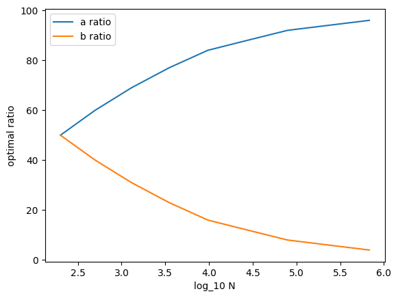
If at training data scale $N^{(1)}=N_{a}^{(1)}+N_{b}^{(1)}=200$, we have optimal domain data composition as $N_{a}^{(1)*}=100,N_{b}^{(1)*}=100$ ($50\%-50\%$); and at scale $N^{(2)}=N_{a}^{(2)}+N_{b}^{(2)}=500$, we have optimal domain data composition as $N_{a}^{(2)*}=300,N_{b}^{(2)*}=200$ ($60\%-40\%$). Then, from the theorem, when the optimal domain data composition has $N_{a}^{(3)*}=(N_{a}^{(2)*})^{2}/N_{a}^{(1)*}=900$, we can predict $N_{b}^{(3)*}=(N_{b}^{(2)*})^{2}/N_{b}^{(1)*}=400$, which gives the optimal ratio at $N^{(3)}=N_{a}^{(3)}+N_{b}^{(3)}=1300$ as $69\%-31\%$.

Similarly,

For $N_{a}^{(4)*}=2700$, we have $N_{b}^{(4)*}=800$, which gives the optimal ratio at $N^{(4)}=3500$ as $77\%-23\%$
For $N_{a}^{(5)*}=8100$, we have $N_{b}^{(5)*}=1600$, which gives the optimal ratio at $N^{(5)}=9700$ as $84\%-16\%$
For $N_{a}^{(6)*}=24300$, we have $N_{b}^{(6)*}=3200$, which gives the optimal ratio at $N^{(6)}=27500$ as $88\%-12\%$
For $N_{a}^{(7)*}=72900$, we have $N_{b}^{(7)*}=6400$, which gives the optimal ratio at $N^{(7)}=79300$ as $92\%-8\%$
For $N_{a}^{(8)*}=218700$, we have $N_{b}^{(8)*}=12800$, which gives the optimal ratio at $N^{(8)}=231500$ as $94\%-6\%$
For $N_{a}^{(9)*}=656100$, we have $N_{b}^{(9)*}=25600$, which gives the optimal ratio at $N^{(9)}=681700$ as $96\%-4\%$

We visualize it in Figure 7.

Figure 7: Illustration: optimal data composition scales in exponential-style functions with training data quantity.

C.2 Scaling Latent Skills

We extend this theory to a general case where the evaluation loss is the perplexity averaged over training domains. Consider the evaluation is composed of a number of indepedent sub-tasks ("latent skills" [25]) which are hidden variables, where each of them observes a power law scaling law relationship with the amount of data contributing to this task ("equivalent data size"), $\mathcal{L}=\mathcal{L}_{0}+\beta_{a}\cdot K_{a}^{-\gamma_{a}}+\beta_{b}\cdot K_{b}^{-\gamma_{b}}+\beta_{c}\cdot K_{c}^{-\gamma_{c}}+\cdots$ where scalar $K_{j}\geq 0$ denote equivalent data size for skill_j, and constants $(\beta_{j},\gamma_{j})\geq 0$ are coefficients associated with skill_j, respectively. Mathematically, these latent skills can be seen as an orthogonal basis that spans the space of evaluation loss.

Consider training data from each domain $D_{i}$ contributes to these skills to varying degrees, where Equivalent data size for skill_j, $K_{j}$, is given as $K_{j}=c_{j,1}\cdot N_{1}+c_{j,2}\cdot N_{2}+\cdots$ where $N_{i}=w_{i}\cdot N$ denotes the amount of training data from domain $D_{i}$ and constant $c_{j,i}$ is the coefficient measuring the degree of contribution between domain $D_{i}$ and skill_j. Defining diagonal matrices for training data composition $\mathbf{N}=diag\{N_{1},N_{2},\cdots\}$ and skill data composition $\mathbf{K}=diag\{K_{a},K_{b},\cdots\}$, we have $\mathbf{K}=\mathbf{A}\mathbf{N}$, where $\mathbf{A}_{ji}=c_{j,i}$ is the matrix for coefficients. For simplicity, we consider training data from each domain will be distributed to the skills such that $\forall i,\sum_{j}N_{i}=1$. This gives the amount of total training data from all domains is identical to the amount of total equivalent data for all skills, $\sum_{j}K_{j}=\sum_{i}N_{i}$. For a training data scale $N=\sum_{i}N_{i}=\sum_{j}K_{j}$, define optimal skill data composition $\mathbf{K^{*}}=diag\{K_{a}^{*},K_{b}^{*},\cdots\}$ as the minimizer of $\mathcal{L}$, given as $\mathbf{K^{*}}={\arg\min}_{\sum_{j}K_{j}=N}\mathcal{L}_{0}+\beta_{a}\cdot K_{a}^{-\gamma_{a}}+\beta_{b}\cdot K_{b}^{-\gamma_{b}}+\cdots$. Theoretically, there can be an infinite number of latent skills. For analysis, we consider a finite number of $k$ independent skills most important for the evaluation. This can considered as performing Principal Components Analysis (PCA) with orthogonal transformation and selecting the first $k$ independent components. We consider the standard scenario with an equal number of relevant skills and data domains where $k=m$ and $\mathbf{A}$ is a square matrix with full rank. This describes the case where this optimization problem is well-defined. We discuss in Appendix C.2 what will happen in other scenarios. In this case, $\mathbf{A}$ is invertible and the corresponding optimal training data composition for $\mathbf{K^{*}}$ can be given as $\mathbf{N^{*}}=\mathbf{A}^{-1}\mathbf{K^{*}}$.

We provide the following theorem, which states that for the scenario described above, optimal training data composition scales in exponential-style functions with training data quantity and can be directly predictable from that of smaller scales without needing to identify the latent skills.

Theorem 2 (Scaling Latent Skills).

Consider the evaluation is composed of a number of indepedent sub-tasks ("latent skills") where each of them observes a power law scaling law relationship with the amount of data contributing to this task ("equivalent data size"). Namely, $\mathcal{L}=\mathcal{L}_{0}+\beta_{a}\cdot K_{a}^{-\gamma_{a}}+\beta_{b}\cdot K_{b}^{-\gamma_{b}}+\beta_{c}\cdot K_{c}^{-\gamma_{c}}+\cdots$ where scalar $K_{j}\geq 0$ denote equivalent data size for skill_j, and constants $(\beta_{j},\gamma_{j})\geq 0$ are coefficients associated with skill_j, respectively. Define diagonal matrices for training data composition $\mathbf{N}=diag\{N_{1},N_{2},\cdots\}$ and skill data composition $\mathbf{K}=diag\{K_{a},K_{b},\cdots\}$. Consider training data from each domain $D_{i}$ contributes to these skills to varying degrees, given as $\mathbf{K}=\mathbf{A}\mathbf{N}$ where $\mathbf{A}_{ji}=c_{j,i}$ is the matrix for coefficients. Assume the amount of total training data from all domains is identical to the amount of total equivalent data for all skills, $\sum_{j}K_{j}=\sum_{i}N_{i}$. Assume there is a finite number of latent skills and data domains and $\mathbf{A}$ is a square matrix with full rank. For a training data scale $N=\sum_{i}N_{i}=\sum_{j}K_{j}$ , define optimal skill data composition $\mathbf{K^{*}}=diag\{K_{a}^{*},K_{b}^{*},\cdots\}$ as the minimizer of $\mathcal{L}$ s.t. $\sum_{j}K_{j}=N$ with corresponding optimal training data composition If we have optimal data compositions $\mathbf{N^{(1)*}}=diag\{N_{a}^{(1)*},N_{b}^{(1)*},\cdots\}$ where its corresponding skill data composition $\mathbf{K^{(1)*}}=diag\{K_{a}^{(1)*},K_{b}^{(1)*},\cdots\}=\mathbf{A}\mathbf{N^{(1)*}}$ minimizes $\mathcal{L}$ s.t. $\sum_{j}K_{j}=\sum_{i}N^{(1)*}=N^{(1)}$, and $\mathbf{N^{(2)*}}=diag\{N_{a}^{(2)*},N_{b}^{(2)*},...\}$ where its corresponding skill data composition $\mathbf{K^{(2)*}}=diag\{K_{a}^{(2)*},K_{b}^{(2)*},...\}=\mathbf{A}\mathbf{N^{(2)*}}$ minimizes $\mathcal{L}$ s.t. $\sum_{j}K_{j}^{(2)*}=\sum_{i}N^{(2)*}=N^{(2)}$ where $N^{(2)}\neq N^{(1)}$, then, other optimal data compositions $\mathbf{N^{(3)*}}=diag\{N_{a}^{(3)*},N_{b}^{(3)*},...\}$ where its corresponding skill data composition $\mathbf{K^{(3)*}}=diag\{K_{a}^{(3)*},K_{b}^{(3)*},\cdots\}=\mathbf{A}\mathbf{N^{(3)*}}$ minimizes $\mathcal{L}$ s.t. $\sum_{j}K_{j}^{(3)*}=\sum_{i}N^{(3)*}=N^{(3)}$ where $N^{(3)}\neq N^{(2)}\neq N^{(1)}$ can be given as $\mathbf{N^{(3)*}}=\mathbf{N^{(2)*}}(\mathbf{N^{(1)*}})^{-1}\mathbf{N^{(2)*}}$.

Proof.

By definition, we have

$$\mathbf{A}\mathbf{N^{(1)*}}=\mathbf{K^{(1)*}},\quad\mathbf{A}\mathbf{N^{(2)*}}=\mathbf{K^{(2)*}},\quad\mathbf{A}\mathbf{N^{(3)*}}=\mathbf{K^{(3)*}}$$

From results of Theorem 1, we have

$$\mathbf{K^{(3)*}}=\mathbf{K^{(2)*}}(\mathbf{K}^{(1)*})^{-1}\mathbf{K^{(2)*}}$$

which gives

$$\mathbf{A}\mathbf{N^{(3)*}}=(\mathbf{A}\mathbf{N^{(2)*}})(\mathbf{A}\mathbf{N^{(1)*}})^{-1}\mathbf{A}\mathbf{N^{(2)*}}$$

Since $\mathbf{A}$ is invertible and $\mathbf{N}$ and $\mathbf{K}$ are diagonal matrices, naturally,

$$(\mathbf{A}\mathbf{N^{(1)*}})^{-1}=(\mathbf{N^{(1)*}})^{-1}\mathbf{A}^{-1}$$

and we have

$$\mathbf{A}\mathbf{N^{(3)*}}=\mathbf{A}\mathbf{N^{(2)*}}[(\mathbf{N^{(1)*}})^{-1}\mathbf{A}^{-1}]\mathbf{A}\mathbf{N^{(2)*}}=\mathbf{A}\mathbf{N^{(2)*}}(\mathbf{N^{(1)*}})^{-1}\mathbf{N^{(2)*}}$$

This directly gives

$$\mathbf{N^{(3)*}}=\mathbf{A}^{-1}\mathbf{A}\mathbf{N^{(2)*}}(\mathbf{N}^{(1)*})^{-1}\mathbf{N^{(2)*}}=\mathbf{N^{(2)*}}(\mathbf{N}^{(1)*})^{-1}\mathbf{N^{(2)*}}$$

which completes the proof.

The above result does not require identifying the latent skills or observing skill data compositions $\mathbf{K}$. Rather, the theorem gives that as long as the coefficient matrix $\mathbf{A}$ is invertible, the scaling of $\mathbf{N}$ complies to the same scaling law as in Section 3.1. ∎

Remark 2 (what happens when $\mathbf{A}$ is not invertible.).

In general, if $\mathbf{A}$ is not invertible, scaling for optimal training data composition is not directly predictable. Specifically, if $\mathbf{A}$ does not have full rank, there exists redundant domains/data sources where their contribution to the skills are identical/exact multipliers of each other. Some data sources may not be needed at any scale; if $\mathbf{A}$ has more rows than columns (more domains than skills), this suggests multiple training data compositions can achieve the same skills data composition and the optimal training data compositions are non-unique (infinitely many). If $\mathbf{A}$ has more columns than rows (more skills than domains), this means there are too many skills to optimize for. No optimal training data composition exists and one has to make trade-offs. If this is relevant to the practical needs, training data may be processed with additional techniques such as clustering and split into more different domains.

Appendix D Experimental Details and Additional Results

D.1 Experimental Details of Section 4.2

Model Training

GPT-2 Large is a variant of the GPT-2 architecture, featuring an embedding dimension of 1280, 36 transformer layers, and 20 attention heads. We rely on the Hugging Face Transformers library for implementation [70]. Specific training hyperparameters are detailed in Table 3.

Architecture	gpt2
Optimizer	AdamW
Tokenizer Vocabulary Size	$50257$
Batch Size Per Device	$1$
Gradient Accumulation Steps	$10$
Maximum Learning Rate	2e-4
LR Schedule	Linear
Weight Decay	1e-2
Warm-up Ratio	$10\%$
Epochs	$3$
GPU Hardware	8x NVIDIA A100/8x NVIDIA H100

Table 3: The list of hyperparameters for GPT-2 Large pretraining.

Dataset Details

The RedPajama dataset is available at: https://huggingface.co/datasets/togethercomputer/RedPajama-Data-1T. The 7 domains involved are characterized as follows:

• Commoncrawl: A vast repository of web-crawled data, providing a heterogeneous mix of internet text.

• C4: The Colossal Clean Crawled Corpus, filtered to remove low-quality content, thus ensuring the reliability and cleanliness of the data.

• GitHub: This domain includes a compilation of publicly available code repositories, offering a rich source of syntactic and semantic patterns inherent in programming languages.

• Books: A collection of textual content from published books, providing diverse narrative styles and complex character developments.

• ArXiv: Comprising scientific papers primarily from the fields of physics, mathematics, computer science, and quantitative biology, this domain offers high-quality, scholarly content.

• Wikipedia: A well-organized and meticulously curated dataset of encyclopedia articles, delivering a broad spectrum of knowledge across multiple disciplines. We only use English samples with ’en’ in meta-data.

• StackExchange: This domain captures a variety of user-generated content from discussions and question-answer sessions across numerous technical topics.

Given copyright restrictions with the Books domain on Hugging Face, we have opted for an alternative source available at https://yknzhu.wixsite.com/mbweb.

For each domain, we ensure only samples with more than 1000 characters are retained. For each sample, the first 1000 characters are truncated, with the exception of the ArXiv and GitHub domains where we randomly extract a continuous block of 1000 characters. For the Wikipedia domain, we keep only those samples that are in English. Samples are selected without replacement, based on the computed data volume for each domain. Additionally, for each domain, a held-out dataset comprising 10K samples is reserved to evaluate the perplexity of the pretrained model.

D.2 Experimental Details of Section 4.3

Model Training

We employ the BERT-base-uncased model from the Hugging Face Transformers library. Originally, BERT’s pretraining scheme involved MLM and next sentence prediction (NSP); however, in our experiments, we exclusively utilize MLM. Detailed training hyperparameters can be found in Table 4.

Architecture	bert-base-uncased
Max Token Length	$300$
Mask Token Percentage	$15$%
Optimizer	AdamW
Batch Size Per Device	$12$
Devices	$4$
Maximum Learning Rate	1e-4
LR Schedule	Linear
Weight Decay	1e-2
Warm-up Steps	$3000$
Epochs	$1\sim 4$
GPU Hardware	4x NVIDIA RTX A6000

Table 4: The list of hyperparameters for BERT pretraining.

Dataset Details

The 5 domains of training data utilized are listed as follows:

• Amazon Reviews: A compilation of customer reviews from Amazon, widely utilized in sentiment analysis studies, available at: https://huggingface.co/datasets/amazon_us_reviews.

• Arxiv: Comprises 1.7 million articles from arXiv, available at: https://www.tensorflow.org/datasets/catalog/scientific_papers.

• Books: A corpus of 11,038 novels by unpublished authors across 16 genres, available at: https://yknzhu.wixsite.com/mbweb.

• Wikipedia: Offers datasets extracted from Wikipedia in various languages, available at: https://www.tensorflow.org/datasets/catalog/wikipedia. We only use English samples with ’en’ in meta-data.

• Open WebText Corpus (OWTC): A corpus of English web texts from Reddit posts, available at: https://skylion007.github.io/OpenWebTextCorpus/.

3 held-out non-training domains used in the evaluation include:

• Pubmed: Features 19,717 diabetes-related publications from the PubMed database, organized into three classes and linked by a network of 44,338 citations, available at: https://www.tensorflow.org/datasets/catalog/scientific_papers

• News: Comprises a significant collection of news articles derived from CommonCrawl, specifically from 5000 news domains indexed by Google News, available at: https://github.com/rowanz/grover/blob/master/realnews/README.md

• GitHub: A curated selection from the RedPajama dataset, this segment includes an array of open-source code projects, available at: https://huggingface.co/datasets/togethercomputer/RedPajama-Data-1T

D.3 Implementation Details of Baselines

Implementation details

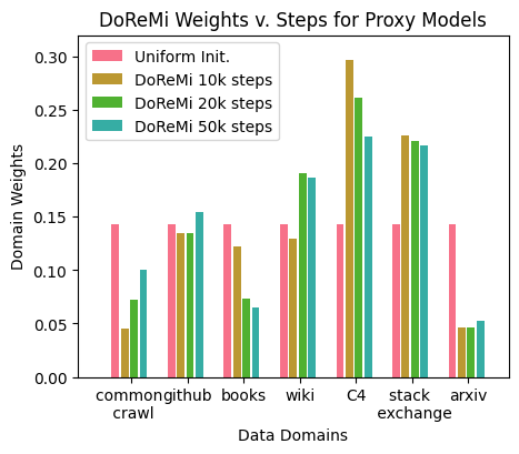
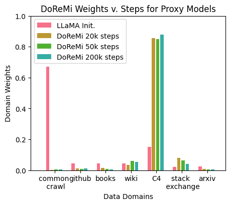
We followed the official implementation of DoReMi for our experiments. We evaluated two sets of reference domain weights: (1) the domain weights utilized in the LLaMA-2 paper [10] (referred to as LLaMA weights), and (2) uniform weights. Both the reference and proxy models have 120M parameters and are trained from scratch. We use GPT-2 tokenizer with a vocabulary size of roughly 50K. For LLaMA weights, we train each model for 20K, 50K and 200K steps for comparison. For uniform weights, we train each model for 10K, 20K and 50K steps. Refer to Table 5 for detailed hyperparameters. The effect of reference weights on the output DoReMi is discussed in Figure10.

Architecture	Decoder-only LM
Max Token Length	$1024$
Optimizer	AdamW
Batch Size Per Device	$8$
Devices	$8$
Maximum Learning Rate	2e-4
LR Schedule	Linear
Weight Decay	1e-2
Warm-up Steps	$3000$
Epochs	$1$
GPU Hardware	8x NVIDIA RTX A6000

Table 5: The list of hyperparameters for DoReMi.

D.4 Evaluation Details

GPT/CLM

The following tasks are considered for downstream performance evaluation, in line with the setup from [12, 37]. For few-shot tasks, the demonstrations are sampled at random.

• BoolQ [29] consists of a question-answering format that requires binary yes/no answers.

• HellaSwag [30] challenges models on their ability to make commonsense inferences.

• PIQA [31] focuses on evaluating a model’s commonsense reasoning regarding physical interactions.

• TruthfulQA [32] is designed to assess the ability of models to generate truthful and factual responses.

• PubMedQA [33] offers a dataset for evaluating question-answering in the biomedical domain.

• CrowsPairs-English [34] tests models on their ability to identify and correct stereotypical biases in English text.

• ARC-Easy [35] presents a set of relatively simpler scientific reasoning questions, aimed at evaluating a model’s basic understanding of scientific principles.

• BigBench-Novel Concepts [36] serves as a test of the model’s creative abstraction skills, challenging it to make sense of scenarios that it could not have memorized during training.

BERT/MLM

For each task, we conduct supervised fine-tuning on the corresponding training data and test the fine-tuned model on the validation data. The hyperparameters for supervised fine-tuning are given in Table 6.

Architecture	bert-base-uncased
Max Token Length	$128$
Batch Size Per Device	$8$ or $300$
Optimizer	AdamW
Devices	$4$
Maximum Learning Rate	2e-5 or 5e-5
Epochs	$3$
GPU Hardware	4x NVIDIA RTX A6000

Table 6: The list of hyperparameters for supervised fine-tuning of BERT.

D.5 Additional Results of Section 4.2

Figure 8 exhibits that AutoScale-predicted weights decreases val loss at least $25\%$ faster than any baseline with up to $37\%$ speed up.

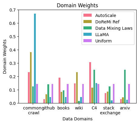
Figure 9 provides a visualization of domain weights used for training GPT-2 Large, given by different methods.

Table 7 examines the domain-specific perplexity of GPT-2 Large trained on 3 billion tokens, respectively. Notably, AutoScale achieves the lowest average validation perplexity and significantly reduces the perplexity in the worst-performing domains.

Figure 10 visualizes DoReMi optimized domain weights with different reference weights and training steps. Training proxy/reference models for different steps gives different weights. It is unclear which weights are optimal. DoReMi recommends 200k steps, which equals >100B tokens in the default setup. Since optimization was conducted relative to the reference weights, reference weights have a profound impact on DoReMi’s output.

Domain/Method	AutoScale	DoReMi (Ref)	Data Mixing	LLaMA	Uniform
			Laws (ref)		(30% more tokens)
Common Crawl	25.598	24.116	30.824	21.464	28.351
Github	7.482	6.678	5.845	7.376	5.784
Books	29.162	33.324	34.450	35.533	31.14
Wikipedia	18.828	17.154	26.795	21.110	19.57
C4	34.242	39.429	38.521	37.393	40.323
Stack Exchange	15.991	15.393	14.519	20.133	13.890
Arxiv	16.558	15.638	12.372	17.598	13.082
Average	21.123	21.676	23.333	22.944	21.736
Worst-domain	34.242	39.429	38.521	37.393	40.323

Table 7: Domain perplexity for 774M Decoder-only LMs trained for 3B tokens. AutoScale notably achieves the lowest average validation perplexity while also significantly decreasing worse-domain perplexity.

(a) Training Decoder-only LMs for 3B tokens.

(b) Training Decoder-only LMs for 5B tokens.

Figure 8: AutoScale-predicted weights decreases val loss at least $25\%$ faster than any baseline with up to $37\%$ speed up. Despite LLaMa weights being very different from uniform weights, they yield highly similar training efficiency at these data scales.

Figure 9: Domain Weights used for training 774M Decoder-only LMs for 3B tokens. (Domain weights for Data Mixing Laws and DoReMi are from references [6] and [5], respectively, which are implemented on the same datasets/data domains with highly similar model architecture/model size/tokenizers.)

(a) with Uniform Reference Weights

(b) with LLaMA Reference Weights (Default)

Figure 10: DoReMi with different reference weights and steps. Training proxy/reference models for different steps gives different weights. It is unclear which weights are optimal. DoReMi recommends 200k steps, which equals >100B tokens in the default setup. Since optimization was conducted relative to the reference weights, reference weights have a profound impact on DoReMi’s output.

D.6 Additional Results of Section 4.3

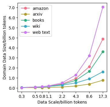
Figure 11 depicts the AutoScale-predicted domain weights for training BERT. It is evident that optimal data quantity for each domain grows in exponential-style functions with training data scale where data sources with diverse samples (e.g., WebText) are upweighted relative to domains with standard format (e.g., ArXiv).

(a) AutoScale-predicted optimal data quantity for each domain as training data scales up.

(b) AutoScale-predicted optimal domain weights as training data scales up.

Figure 11: AutoScale-predicted domain weights for training Encoder-only LMs (BERT). Optimal data quantity for each domain grows in exponential-style functions with training data scale (left) where data sources with diverse samples (e.g., WebText) are upweighted relative to domains with standard format (e.g., ArXiv).

D.7 Runtime Analysis

Training a GPT-2 large model from scratch for 3B tokens requires 15.5 hours on 8x NVIDIA A100 40GB SXM GPUs or 9 hours on 8x NVIDIA H100 80GB GPUs. Training time increases linearly with the number of training tokens on both types of GPUs.

Training BERT-base models takes 2 hours for every 18k steps on 4x NVIDIA A6000 48GB GPUs. Computational time grows linearly with the number of training steps.

Training reference models for DoReMi takes one hour for every 10K steps on 8x NVIDIA A6000 48GB GPUs. Computational time grows linearly with the number of training steps. Similar runtime for training proxy models for DoReMi.

References

- [1] Sang Michael Xie, Hieu Pham, Xuanyi Dong, Nan Du, Hanxiao Liu, Yifeng Lu, Percy S Liang, Quoc V Le, Tengyu Ma, and Adams Wei Yu. Doremi: Optimizing data mixtures speeds up language model pretraining. Advances in Neural Information Processing Systems, 36, 2024.
- [2] Mayee Chen, Nicholas Roberts, Kush Bhatia, Jue Wang, Ce Zhang, Frederic Sala, and Christopher Ré. Skill-it! a data-driven skills framework for understanding and training language models. Advances in Neural Information Processing Systems, 36, 2024.
- [3] Alon Albalak, Liangming Pan, Colin Raffel, and William Yang Wang. Efficient online data mixing for language model pre-training. arXiv preprint arXiv:2312.02406, 2023.
- [4] Luca Soldaini, Rodney Kinney, Akshita Bhagia, Dustin Schwenk, David Atkinson, Russell Authur, Ben Bogin, Khyathi Chandu, Jennifer Dumas, Yanai Elazar, et al. Dolma: An open corpus of three trillion tokens for language model pretraining research. arXiv preprint arXiv:2402.00159, 2024.
- [5] Simin Fan, Matteo Pagliardini, and Martin Jaggi. Doge: Domain reweighting with generalization estimation. arXiv preprint arXiv:2310.15393, 2023.
- [6] Jiasheng Ye, Peiju Liu, Tianxiang Sun, Yunhua Zhou, Jun Zhan, and Xipeng Qiu. Data mixing laws: Optimizing data mixtures by predicting language modeling performance. arXiv preprint arXiv:2403.16952, 2024.
- [7] Shiori Sagawa, Pang Wei Koh, Tatsunori B Hashimoto, and Percy Liang. Distributionally robust neural networks for group shifts: On the importance of regularization for worst-case generalization. arXiv preprint arXiv:1911.08731, 2019.
- [8] Sachin Goyal, Pratyush Maini, Zachary Chase Lipton, Aditi Raghunathan, and J Zico Kolter. The science of data filtering: Data curation cannot be compute agnostic. In ICLR 2024 Workshop on Navigating and Addressing Data Problems for Foundation Models.
- [9] Jiahao Wang, Bolin Zhang, Qianlong Du, Jiajun Zhang, and Dianhui Chu. A survey on data selection for llm instruction tuning. arXiv preprint arXiv:2402.05123, 2024.
- [10] Hugo Touvron, Thibaut Lavril, Gautier Izacard, Xavier Martinet, Marie-Anne Lachaux, Timothée Lacroix, Baptiste Rozière, Naman Goyal, Eric Hambro, Faisal Azhar, et al. Llama: Open and efficient foundation language models. arXiv preprint arXiv:2302.13971, 2023.
- [11] Leo Gao, Stella Biderman, Sid Black, Laurence Golding, Travis Hoppe, Charles Foster, Jason Phang, Horace He, Anish Thite, Noa Nabeshima, et al. The pile: An 800gb dataset of diverse text for language modeling. arXiv preprint arXiv:2101.00027, 2020.
- [12] Sachin Mehta, Mohammad Hossein Sekhavat, Qingqing Cao, Maxwell Horton, Yanzi Jin, Chenfan Sun, Iman Mirzadeh, Mahyar Najibi, Dmitry Belenko, Peter Zatloukal, et al. Openelm: An efficient language model family with open-source training and inference framework. arXiv preprint arXiv:2404.14619, 2024.
- [13] Together Computer. Redpajama: An open source recipe to reproduce llama training dataset, 2023.
- [14] Brandon McKinzie, Zhe Gan, Jean-Philippe Fauconnier, Sam Dodge, Bowen Zhang, Philipp Dufter, Dhruti Shah, Xianzhi Du, Futang Peng, Floris Weers, et al. Mm1: Methods, analysis & insights from multimodal llm pre-training. arXiv preprint arXiv:2403.09611, 2024.
- [15] Jack W Rae, Sebastian Borgeaud, Trevor Cai, Katie Millican, Jordan Hoffmann, Francis Song, John Aslanides, Sarah Henderson, Roman Ring, Susannah Young, et al. Scaling language models: Methods, analysis & insights from training gopher. arXiv preprint arXiv:2112.11446, 2021.
- [16] Ben Sorscher, Robert Geirhos, Shashank Shekhar, Surya Ganguli, and Ari Morcos. Beyond neural scaling laws: beating power law scaling via data pruning. Advances in Neural Information Processing Systems, 35:19523–19536, 2022.
- [17] Alec Radford, Jeffrey Wu, Rewon Child, David Luan, Dario Amodei, Ilya Sutskever, et al. Language models are unsupervised multitask learners. OpenAI blog, 1(8):9, 2019.
- [18] Jacob Devlin, Ming-Wei Chang, Kenton Lee, and Kristina Toutanova. Bert: Pre-training of deep bidirectional transformers for language understanding. arXiv preprint arXiv:1810.04805, 2018.
- [19] Alex Wang, Amanpreet Singh, Julian Michael, Felix Hill, Omer Levy, and Samuel Bowman. Glue: A multi-task benchmark and analysis platform for natural language understanding. In Proceedings of the 2018 EMNLP Workshop BlackboxNLP: Analyzing and Interpreting Neural Networks for NLP, pages 353–355, 2018.
- [20] Pranav Rajpurkar, Jian Zhang, Konstantin Lopyrev, and Percy Liang. Squad: 100,000+ questions for machine comprehension of text. arXiv preprint arXiv:1606.05250, 2016.
- [21] Risheng Liu, Jiaxin Gao, Jin Zhang, Deyu Meng, and Zhouchen Lin. Investigating bi-level optimization for learning and vision from a unified perspective: A survey and beyond. IEEE Transactions on Pattern Analysis and Machine Intelligence, 44(12):10045–10067, 2021.
- [22] Jared Kaplan, Sam McCandlish, Tom Henighan, Tom B Brown, Benjamin Chess, Rewon Child, Scott Gray, Alec Radford, Jeffrey Wu, and Dario Amodei. Scaling laws for neural language models. arXiv preprint arXiv:2001.08361, 2020.
- [23] Danny Hernandez, Jared Kaplan, Tom Henighan, and Sam McCandlish. Scaling laws for transfer. arXiv preprint arXiv:2102.01293, 2021.
- [24] Dimitri P Bertsekas. Nonlinear programming. Journal of the Operational Research Society, 48(3):334–334, 1997.
- [25] Anthony Tiong, Junqi Zhao, Junnan Li, Steven Hoi, Caiming Xiong, and Boyang Li. Toward data-driven skill identification for general-purpose vision-language models. In ICLR 2024 Workshop on Navigating and Addressing Data Problems for Foundation Models.
- [26] Colin Raffel, Noam Shazeer, Adam Roberts, Katherine Lee, Sharan Narang, Michael Matena, Yanqi Zhou, Wei Li, and Peter J Liu. Exploring the limits of transfer learning with a unified text-to-text transformer. Journal of machine learning research, 21(140):1–67, 2020.
- [27] Jacob Devlin, Ming-Wei Chang, Kenton Lee, and Kristina Toutanova. BERT: pre-training of deep bidirectional transformers for language understanding. CoRR, abs/1810.04805, 2018.
- [28] Aaron Gokaslan and Vanya Cohen. Openwebtext corpus. http://Skylion007.github.io/OpenWebTextCorpus, 2019.
- [29] Christopher Clark, Kenton Lee, Ming-Wei Chang, Tom Kwiatkowski, Michael Collins, and Kristina Toutanova. Boolq: Exploring the surprising difficulty of natural yes/no questions. arXiv preprint arXiv:1905.10044, 2019.
- [30] Rowan Zellers, Ari Holtzman, Yonatan Bisk, Ali Farhadi, and Yejin Choi. Hellaswag: Can a machine really finish your sentence? arXiv preprint arXiv:1905.07830, 2019.
- [31] Yonatan Bisk, Rowan Zellers, Jianfeng Gao, Yejin Choi, et al. Piqa: Reasoning about physical commonsense in natural language. In Proceedings of the AAAI conference on artificial intelligence, volume 34, pages 7432–7439, 2020.
- [32] Stephanie Lin, Jacob Hilton, and Owain Evans. Truthfulqa: Measuring how models mimic human falsehoods. arXiv preprint arXiv:2109.07958, 2021.
- [33] Qiao Jin, Bhuwan Dhingra, Zhengping Liu, William W Cohen, and Xinghua Lu. Pubmedqa: A dataset for biomedical research question answering. arXiv preprint arXiv:1909.06146, 2019.
- [34] Nikita Nangia, Clara Vania, Rasika Bhalerao, and Samuel R Bowman. Crows-pairs: A challenge dataset for measuring social biases in masked language models. arXiv preprint arXiv:2010.00133, 2020.
- [35] Peter Clark, Isaac Cowhey, Oren Etzioni, Tushar Khot, Ashish Sabharwal, Carissa Schoenick, and Oyvind Tafjord. Think you have solved question answering? try arc, the ai2 reasoning challenge. arXiv preprint arXiv:1803.05457, 2018.
- [36] Aarohi Srivastava, Abhinav Rastogi, Abhishek Rao, Abu Awal Md Shoeb, Abubakar Abid, Adam Fisch, Adam R Brown, Adam Santoro, Aditya Gupta, Adrià Garriga-Alonso, et al. Beyond the imitation game: Quantifying and extrapolating the capabilities of language models. arXiv preprint arXiv:2206.04615, 2022.
- [37] Samir Yitzhak Gadre, Georgios Smyrnis, Vaishaal Shankar, Suchin Gururangan, Mitchell Wortsman, Rulin Shao, Jean Mercat, Alex Fang, Jeffrey Li, Sedrick Keh, et al. Language models scale reliably with over-training and on downstream tasks. arXiv preprint arXiv:2403.08540, 2024.
- [38] Leo Gao, Jonathan Tow, Stella Biderman, Sid Black, Anthony DiPofi, Charles Foster, Laurence Golding, Jeffrey Hsu, Kyle McDonell, Niklas Muennighoff, et al. A framework for few-shot language model evaluation. Version v0. 0.1. Sept, 2021.
- [39] Ibrahim M Alabdulmohsin, Behnam Neyshabur, and Xiaohua Zhai. Revisiting neural scaling laws in language and vision. Advances in Neural Information Processing Systems, 35:22300–22312, 2022.
- [40] Jordan Hoffmann, Sebastian Borgeaud, Arthur Mensch, Elena Buchatskaya, Trevor Cai, Eliza Rutherford, Diego de Las Casas, Lisa Anne Hendricks, Johannes Welbl, Aidan Clark, et al. Training compute-optimal large language models. arXiv preprint arXiv:2203.15556, 2022.
- [41] AI@Meta. Llama 3 model card. 2024.
- [42] Yasaman Bahri, Ethan Dyer, Jared Kaplan, Jaehoon Lee, and Utkarsh Sharma. Explaining neural scaling laws. arXiv preprint arXiv:2102.06701, 2021.
- [43] Cody Coleman, Christopher Yeh, Stephen Mussmann, Baharan Mirzasoleiman, Peter Bailis, Percy Liang, Jure Leskovec, and Matei Zaharia. Selection via proxy: Efficient data selection for deep learning. arXiv preprint arXiv:1906.11829, 2019.
- [44] Vishal Kaushal, Rishabh Iyer, Suraj Kothawade, Rohan Mahadev, Khoshrav Doctor, and Ganesh Ramakrishnan. Learning from less data: A unified data subset selection and active learning framework for computer vision. In 2019 IEEE Winter Conference on Applications of Computer Vision (WACV), pages 1289–1299. IEEE, 2019.
- [45] Krishnateja Killamsetty, Sivasubramanian Durga, Ganesh Ramakrishnan, Abir De, and Rishabh Iyer. Grad-match: Gradient matching based data subset selection for efficient deep model training. In International Conference on Machine Learning, pages 5464–5474. PMLR, 2021.
- [46] Sören Mindermann, Jan M Brauner, Muhammed T Razzak, Mrinank Sharma, Andreas Kirsch, Winnie Xu, Benedikt Höltgen, Aidan N Gomez, Adrien Morisot, Sebastian Farquhar, et al. Prioritized training on points that are learnable, worth learning, and not yet learnt. In International Conference on Machine Learning, pages 15630–15649. PMLR, 2022.
- [47] Chanho Park, Rehan Ahmad, and Thomas Hain. Unsupervised data selection for speech recognition with contrastive loss ratios. In ICASSP 2022-2022 IEEE International Conference on Acoustics, Speech and Signal Processing (ICASSP), pages 8587–8591. IEEE, 2022.
- [48] Andrew Rosenberg, Bhuvana Ramabhadran, Yu Zhang, and Murali Karthick Baskar. Guided data selection for masked speech modeling, April 6 2023. US Patent App. 17/820,871.
- [49] Roee Aharoni and Yoav Goldberg. Unsupervised domain clusters in pretrained language models. arXiv preprint arXiv:2004.02105, 2020.
- [50] Tom Brown, Benjamin Mann, Nick Ryder, Melanie Subbiah, Jared D Kaplan, Prafulla Dhariwal, Arvind Neelakantan, Pranav Shyam, Girish Sastry, Amanda Askell, et al. Language models are few-shot learners. Advances in neural information processing systems, 33:1877–1901, 2020.
- [51] Suchin Gururangan, Ana Marasović, Swabha Swayamdipta, Kyle Lo, Iz Beltagy, Doug Downey, and Noah A Smith. Don’t stop pretraining: Adapt language models to domains and tasks. arXiv preprint arXiv:2004.10964, 2020.
- [52] Sang Michael Xie, Shibani Santurkar, Tengyu Ma, and Percy Liang. Data selection for language models via importance resampling. arXiv preprint arXiv:2302.03169, 2023.
- [53] Aakanksha Chowdhery, Sharan Narang, Jacob Devlin, Maarten Bosma, Gaurav Mishra, Adam Roberts, Paul Barham, Hyung Won Chung, Charles Sutton, Sebastian Gehrmann, et al. Palm: Scaling language modeling with pathways. arXiv preprint arXiv:2204.02311, 2022.
- [54] Feiyang Kang, Hoang Anh Just, Yifan Sun, Himanshu Jahagirdar, Yuanzhi Zhang, Rongxing Du, Anit Kumar Sahu, and Ruoxi Jia. Get more for less: Principled data selection for warming up fine-tuning in llms. 12th International Conference on Learning Representations, ICLR, 2024.
- [55] Alexander Wettig, Aatmik Gupta, Saumya Malik, and Danqi Chen. Qurating: Selecting high-quality data for training language models. arXiv preprint arXiv:2402.09739, 2024.
- [56] Pratyush Maini, Skyler Seto, He Bai, David Grangier, Yizhe Zhang, and Navdeep Jaitly. Rephrasing the web: A recipe for compute and data-efficient language modeling. arXiv preprint arXiv:2401.16380, 2024.
- [57] Christoph Schuhmann, Richard Vencu, Romain Beaumont, Robert Kaczmarczyk, Clayton Mullis, Aarush Katta, Theo Coombes, Jenia Jitsev, and Aran Komatsuzaki. Laion-400m: Open dataset of clip-filtered 400 million image-text pairs. arXiv preprint arXiv:2111.02114, 2021.
- [58] Rafid Mahmood, James Lucas, David Acuna, Daiqing Li, Jonah Philion, Jose M Alvarez, Zhiding Yu, Sanja Fidler, and Marc T Law. How much more data do i need? estimating requirements for downstream tasks. In Proceedings of the IEEE/CVF Conference on Computer Vision and Pattern Recognition, pages 275–284, 2022.
- [59] Rafid Mahmood, James Lucas, Jose M Alvarez, Sanja Fidler, and Marc Law. Optimizing data collection for machine learning. Advances in Neural Information Processing Systems, 35:29915–29928, 2022.
- [60] Feiyang Kang, Hoang Anh Just, Anit Kumar Sahu, and Ruoxi Jia. Performance scaling via optimal transport: Enabling data selection from partially revealed sources. arXiv preprint arXiv:2307.02460, 2023.
- [61] Hoang Anh Just, I-Fan Chen, Feiyang Kang, Yuanzhi Zhang, Anit Kumar Sahu, and Ruoxi Jia. Asr data selection from multiple sources: A practical approach on performance scaling. NeurIPS 2023 Workshop on Efficient Natural Language and Speech Processing (ENLSP), 2023.
- [62] Zalán Borsos, Mojmir Mutny, and Andreas Krause. Coresets via bilevel optimization for continual learning and streaming. Advances in Neural Information Processing Systems, 33:14879–14890, 2020.
- [63] Baharan Mirzasoleiman, Jeff Bilmes, and Jure Leskovec. Coresets for data-efficient training of machine learning models. In International Conference on Machine Learning, pages 6950–6960. PMLR, 2020.
- [64] Ruoxi Jia, David Dao, Boxin Wang, Frances Ann Hubis, Nezihe Merve Gurel, Bo Li, Ce Zhang, Costas J Spanos, and Dawn Song. Efficient task-specific data valuation for nearest neighbor algorithms. arXiv preprint arXiv:1908.08619, 2019.
- [65] Amirata Ghorbani and James Zou. Data shapley: Equitable valuation of data for machine learning. In International Conference on Machine Learning, pages 2242–2251. PMLR, 2019.
- [66] Pang Wei Koh and Percy Liang. Understanding black-box predictions via influence functions. In International conference on machine learning, pages 1885–1894. PMLR, 2017.
- [67] Hoang Anh Just, Feiyang Kang, Tianhao Wang, Yi Zeng, Myeongseob Ko, Ming Jin, and Ruoxi Jia. Lava: Data valuation without pre-specified learning algorithms. In 11th International Conference on Learning Representations, ICLR, page to appear, 2023.
- [68] Yongchan Kwon and James Zou. Data-oob: Out-of-bag estimate as a simple and efficient data value. arXiv preprint arXiv:2304.07718, 2023.
- [69] Stephanie Schoch, Ritwick Mishra, and Yangfeng Ji. Data selection for fine-tuning large language models using transferred shapley values. arXiv preprint arXiv:2306.10165, 2023.
- [70] Thomas Wolf, Lysandre Debut, Victor Sanh, Julien Chaumond, Clement Delangue, Anthony Moi, Pierric Cistac, Tim Rault, Rémi Louf, Morgan Funtowicz, et al. Huggingface’s transformers: State-of-the-art natural language processing. arXiv preprint arXiv:1910.03771, 2019.
[sections] \printcontents[sections]l1