Non-standard boundary behaviour in binary mixture models
Abstract
Consider a binary mixture model of the form , where is standard Gaussian and is a completely specified heavy-tailed distribution with the same support. For a sample of independent and identically distributed values , the maximum likelihood estimator is asymptotically normal provided that is an interior point. This paper investigates the large-sample behaviour for boundary points, which is entirely different and strikingly asymmetric for and . The reason for the asymmetry has to do with typical choices such that is an extreme boundary point and is usually not extreme. On the right boundary, well known results on boundary parameter problems are recovered, giving . On the left boundary, , where indexes the domain of attraction of the density ratio when . For , which is the most important case in practice, we show how the tail behaviour of governs the rate at which tends to zero. A new limit theorem for the joint distribution of the sample maximum and sample mean conditional on positivity establishes multiple inferential anomalies. Most notably, given , the likelihood ratio statistic has a conditional null limit distribution that is not , but is determined by the joint limit theorem.
Some key words: -stable limit law; binary mixture; boundary point; empirical Bayes; multiple testing; non-standard likelihood theory; parametrization.
1 Introduction
Let be distinct probability distributions on the same measurable space. For each , the mixture
| (1) |
is also a probability distribution on the same space. In this paper, the phrase “mixture model generated by ” is interpreted as the set of convex combinations
in which the generators are the boundary points.
The model (1) arises particularly in connection with the empirical Bayes approach to multiple testing (Efron et al., 2001), where interest is either in evaluating the simultaneous correctness of a set of statements concerning the same null hypothesis, or in the assessment of different null hypotheses, at most a small number of which are false. The case in which one of the components is standard Gaussian reflects a reduction by sufficiency to a set of pivotal test statistics and is particularly relevant for the applications we have in mind. The other component is typically chosen to have tails that are heavier than Gaussian, for instance a standard Gaussian convolution corresponding to a signal plus noise model at the relevant site. Any given statistic is either from or and an arbitrary statistic is treated as a draw from for some on account of the label being unknown.
The goal of this paper is to study the large-sample behaviour of the maximum-likelihood estimator and related statistics when the generators have the same support and the data are generated independently according to the boundary distribution . In that case, we write for the density ratio at . For , the error probability has a large-sample limit, which is strictly positive in certain cases, and zero in other cases. It is shown in section 3 that is zero if and only if the random variables belong to the domain of attraction of the Cauchy class, i.e., the -stable family with index . Otherwise, if belongs to the the domain of attraction of any non-Cauchy class, which necessarily has index , the limit probability is strictly positive but not more than one half.
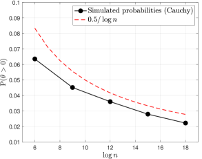
For reasons that are explained in section 2.5, the Cauchy class is virtually the default in practical work with mixtures where the null generator is Gaussian and is symmetric with heavier tails. In such situations, it is of interest to characterize the rate at which the error tends to zero. For example, if has regularly-varying tails with index , e.g., for large , then the rate is logarithmic:
By contrast, if has exponential tails, e.g., for large and , then
Hereafter, denotes the probability with respect to the null generator or its -fold product .
An important new result is the limit distribution of the likelihood ratio statistic conditional on . The derivation is based on a new limit theorem establishing a large-sample joint distribution for the sample mean and sample maximum of a random variable in the Cauchy domain of attraction, conditional on positivity of the sample mean. The theorem may be of interest in its own right but here we focus on its implications for multiple testing.
2 Maximum likelihood
2.1 Regularity conditions
Under the model (1), are independent random variables with distribution for some . Standard theory for maximum-likelihood estimators tells us that, under suitable regularity conditions, has a zero-mean Gaussian limit. A principal regularity condition is that all distributions in the model have the same support. This condition need not be satisfied by , but it is automatic for the sub-model in which . Whether and have the same support or not, a second principal regularity condition requires to be an interior point. Otherwise, if , the event has positive probability, so the limit distribution cannot be Gaussian. The mixture model can therefore be regular only if the boundary points are excluded. As discussed in section 2.4, from a list of further regularity conditions, there is the possibility that others are violated. In the empirical Bayes formulations that motivated the present work, non-existence of second moments presents considerable challenges not covered by existing literature on boundary inference problems.
2.2 Unequal supports
For completeness, we consider briefly the case where the supports and are not equal. The qualitative behaviour of the maximum-likelihood estimator is conveniently illustrated by an example in which is uniform on and is uniform on . The likelihood function is
where is the number of sample points in the interval . In the null case , we have and
Thus, at an exponential rate.
The generators are said to have disjoint supports if there exist disjoint events such that . By modifying the preceding example so that either the distributions have disjoint supports or is a subset of , we find with -probability one for every . By contrast, if is a proper subset of , we find that .
It appears from this analysis that the null error rate has a large-sample limit, which is either zero or one half.
2.3 Equal supports
In the standard case, the generators share a common support and have positive densities , so that has density , which is linear in . The contribution to the log likelihood from a single observation at is strictly concave as a function of , and the sum is also strictly concave. Consequently the maximum-likelihood estimate is either a stationary point or a boundary point.
The log likelihood derivative is
and where is the density ratio of the boundary points. It follows that the event is the same as the event , where are independently distributed as . In other words, if and only if the sample average of the transformed variables exceeds its expected value
If has a finite second moment , then is zero-mean Gaussian for large , and by the law of large numbers. In this case with probability 1/2 in the large-sample limit; otherwise is half-Gaussian with scale parameter . This is the familiar boundary-parameter result established by other authors (e.g. Chernoff, 1954; Liang and Self, 1987; Geyer, 1994). The boundary probabilities exhibit more interesting behaviours in the cases for which does not have a finite second moment under the null model. It is those situations that we explore here.
2.4 Position within the literature
The inferential problem for binary mixtures belongs to a class of boundary problems for which an extensive literature was carefully surveyed by Brazzale and Mameli (2024). Appendix A.1 of that work outlines an argument due to Liang and Self (1987) establishing the limit distribution of the log likelihood ratio statistic when the true value of the parameter is on the boundary. Two aspects of the argument are problematic when does not have finite variance under the null distribution : that the Fisher information at is not finite, being the expectation of ; and that a suitably rescaled version of is not asymptotically normally distributed. The same issues afflict the argument of Ghosh and Sen (1985) presented in Appendix A.3 of Brazzale and Mameli (2024). Non-existence of second moments necessitates a radically different approach based on the theory of -stable limits (Gnedenko and Kolmogorov, 1954) and regular variation (Bingham, Goldie and Teugels, 1987). From this we are able to delineate the role of tail properties in determining the null error rate and the anomalous limiting behaviour of likelihood-based statistics.
2.5 Tail behaviour for Gaussian mixtures
The motivating example for a large part of this paper is a restricted class of binary Gaussian mixtures in which the density ratio is an even function that is continuous, unbounded and ultimately monotone. Ultimate monotonicity means that to each sufficiently large there corresponds a number such that
| (2) |
By Mills’s approximation to the Gaussian tail probability and the implicit definition ,
| (3) |
It follows that the asymptotic inverse relationship determines the null tail behaviour via , and thereby the limit distribution of normalized sums.
For a large class of non-null generators, including all whose density satisfies
| (4) |
for some and slowly-varying , we find that as . This asymptotic inverse implies
where, for every in the class (4), is also slowly varying. In all such cases, the random variable , or more correctly, its distribution, belongs to the Cauchy domain of attraction with index .
3 Limit distributions for sums
3.1 Stable limits
The theory of limit distributions for the sum of independent and identically distributed random variables is tied up with distributional stability of convolutions. Modulo affine transformation, the stable distributions are indexed by two parameters: an index and a skewness parameter . Every stable distribution with has a density that is strictly positive on the real line; only in a few cases is it possible to express the density in terms of standard functions. However, the characteristic function of every limit distribution is necessarily of the form where
See Bingham, Goldie and Teugels (1987, Theorem 8.3.2), or Gnedenko and Kolmogorov (1954, chapter 34) (where the sign of is reversed for ).
Note that not all -combinations give rise to distinct distributions. In the Gaussian case () the last version of the log characteristic function reduces to , so is immaterial and all limits are symmetric. However, limits in every other class are symmetric only if .
Zolotarev (1986, section 2.5) gives the tail behaviour of the -limit distribution parameterized according to the characteristic function shown above:
where and . See also Feller (1966, section XVII.6). For , the first limit is interpreted as ; likewise for in the second limit. Note that , so this characterization is correct but not tight for Gaussian limits. For completeness, we include a derivation of the above expression for the tail probability when in Appendix III.
For the binary mixture problems considered in this paper, the class of limit distributions that can arise is a proper subset of those listed above. First, the fact that each summand has finite mean implies . Second, the fact that the random variables are positive implies maximal skewness with . For , equation (2.2.30) of Zolotarev (1986) gives
| (5) | ||||
which reduces to for .
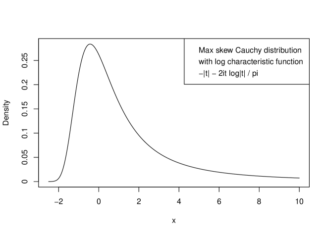
In the asymmetric Cauchy class, the distribution with log characteristic function
has the maximally skew density,
| (6) |
which is shown in Fig. 1. Although the summands have finite mean, the characteristic function for does not have a first-order Taylor expansion so the limit distribution does not have a first moment. The left tail is sub-Cauchy and ; the right tail behaviour is or , where .
3.2 Stabilizing sequences
More generally, let be the cumulative function of a distribution on the positive real line, and let be the right-tail probability. In order that belong to the domain of attraction of a stable law with index , it is necessary and sufficient that the tail be regularly varying, i.e.,
| (7) |
for large and some slowly-varying function . This is a re-statement of a special case of Theorem 2 from section 35 of Gnedenko and Kolmogorov (1954). For the moment, the choice of constant is immaterial, but the particular choice
| (8) |
matching the right tail of the limit distribution, will subsequently be convenient.
Note that the slow-variation factor in (7) is expressed deliberately in the form rather than or . This choice simplifies the scaling sequence (10). More obviously, if is a random variable whose tail is regularly-varying with index and slowly-varying function , then the transformed variable has a regularly-varying tail with index and the same function . In particular, implies for .
Let be independent and identically distributed with distribution in the domain of attraction of some stable law with index . Then there exist stabilizing sequences such that
has the stable limit distribution with index . The skewness coefficient is a balance between the two tails: if the support of is bounded below, then . For , the scaling coefficients are . Otherwise, for , they are determined by the condition
for each (Gnedenko and Kolmogorov, 1954, section 35). This implies
To each slowly varying function there corresponds a function , called the de Bruijn conjugate, which is defined up to asymptotic equivalence by the condition
| (9) |
If we now set , the condition on reduces to , which implies that , and hence
| (10) |
For a proof of equation (9), see Theorem 1.5.23 of Bingham, Goldie and Teugels (1987). Conjugation is an involution , which is also a group inverse under the compositional operation discussed in Appendix I. For the moment, it suffices to remark that if for any real and , then . In general, however, the conjugate is not equivalent to the reciprocal, and the conjugate of a functional product is not the product of the conjugates.
For , the distribution in (7) has a finite mean , and the footnote to Theorem 2 in section 35 of Gnedenko and Kolmogorov (1954) gives the centering sequence , which implies that
has the stable limit distribution discussed in the preceding section. It follows from (5) that the exceedance event has a large-sample limit probability
| (11) |
which is strictly positive, but not more than one half. The case does not arise in mixture models and is not discussed here.
The single remaining case is a little more complicated because even if the mean is finite. The development in section 2.5 shows that it is also by far the most important case for Gaussian mixture models.
3.3 Stabilizing sequences for Cauchy limits
In order for a distribution with tail probability to have a finite mean, it is necessary and sufficient that the tail contribution be finite. Integration by parts gives
For example, suffices for finiteness only if . While both terms tend to zero for large , the second term is dominant.
For , the scaling sequence (10) is . Finiteness of the mean implies , and hence as . The centering sequence given explicitly in the footnote to Theorem 2 of Gnedenko and Kolmogorov (1954) is
See also equation (6) in Chow and Teugels (1979). We now find an approximation for this sine-integral for a broad class of functions , conveniently parametrized in order to recover the most important cases arising in Gaussian mixture models.
Theorem 3.1.
Let be a finite-mean distribution on the positive real line whose tail is , where and
is slowly varying and . Finiteness of the mean implies either and , or and . With the convention that when and , the sine-integral for large is, in either case,
where is the mean, for , and .
Proof.
The argument detailed in Appendix II shows that the dominant component of the sine-integral for small is
where the remainder is of smaller order than the second term.
For , the second part is a straightforward integral
For , the transformation gives rise to a gamma-tail integral
∎
Corollary 3.1.
For a distribution satisfying the conditions of the preceding theorem, the centering sequence is
The third line follows from the definition of the de Bruijn conjugate in (9).
Corollary 3.2.
The large-sample distribution of the sample average is
where has the Cauchy limit with skewness . Given the right-tail behaviour of the limit distribution,
tending to zero at rate if , or if .
3.4 Joint distribution of
Let be a zero-mean distribution with support and tail satisfying the conditions of Theorem 3.1, and let be an iid sample. Our goal in this section is to prove the following theorem concerning the joint distribution of the sample average and the maximum order statistic .
Theorem 3.2.
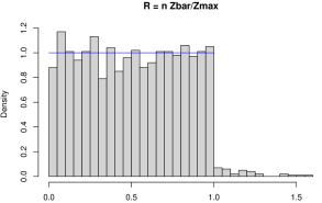
Let . Given , the conditional limit distribution of is such that
where is uniform on . It follows that is conditionally self-reciprocal, the ratio is conditionally uniform, and the support of the joint distribution degenerates to the line .
Remark 3.1.
The unconditional scaling factor for both and is , so has a joint limit distribution, which has been studied by Chow and Teugels (1979) in this setting. However, the conditioning event has probability tending to zero, so the joint limit distribution does not determine the limit of conditional distributions. Theorem 3.2 implies that and are asymptotically equivalent events for each .
To prove the theorem, we first state a technical lemma that relates the sample mean to the sample maximum in the event where the latter is unusually large.
Lemma 3.1.
Proof.
Let be the th order statistic with . Since the transformed variables are independent uniform, the joint distribution of the top order statistics is such that successive differences of the probability-integral transformed values
have exactly the same distribution as successive spacings of the top of independent uniform order statistics. For large and this implies that are independent unit exponential variables. For , the inverse function is and
| (13) |
where . If for some , then is unusually small compared with , so that . It follows that the conditional distribution of given is approximately the same as the unconditional distribution of . In that event, Corollary 3.2 implies
| (14) |
which implies (12). For , implies
∎
Proof of Theorem 3.2.
4 Implications for Gaussian mixtures
4.1 Parametrization for binary mixtures
When the null density is centered at the origin, it is common in the empirical Bayes approach to multiple testing to attribute all observations near zero to the null. This “zero-assumption” means , and ensures identifiability of the parameters and (see, e.g. Chapter 4.5 of Efron, 2012).
When the zero assumption does not hold there may exist real numbers or such that remains a valid probability density. Consider the set of all such , for which the extreme points are
When has heavier tails than , the extreme points typically satisfy and , and the original model is a strict subset of the extended model
| (16) |
The parameter space that is superficially natural from a modelling point of view is often artificial in the relevant mathematical sense. This extension of the parameter space for is illustrated for two Gaussian mixture problems in examples 4.1 and 4.2 below.
The extended model was considered by various authors (see, e.g. Genovese and Wasserman (2004), Patra and Sen (2016) and references therein) in a multiple testing context in order to provide inference for the non-null proportion, i.e. the mixing parameter in our setup. Patra and Sen (2016) point out that when for some constant , some of the probability mass in can be re-assigned to the null component without changing the density of the overall mixture. To address this non-identifiability issue, the latter authors define the minimal value
where is the marginal cdf, and propose an estimator , defined by a non-random sequence , whose error probability under the global null tends to zero, i.e. . In the current work, corresponds to in the extended model (16), which is consistently estimated by maximizing the likelihood over the extended parameter space. However, as equation (11) shows, the maximum likelihood estimator can be inconsistent when .
That and are respectively extreme and non-extreme boundary points of the extended model (16) leads to strikingly asymmetric boundary behaviour of the maximum likelihood estimator when the data are independent draws from and respectively. Under , is an interior point and the density ratio has finite variance. It follows from section 2.3 that the error probability tends to 1/2 as by the central limit theorem; this reflects known results from the literature on boundary inference problems. The behaviour under is non-standard because is an extreme boundary point. As explained in sections 2.3 and 2.5, the boundary behaviour is characterized by the tail probability of induced by the upper tail of .
Example 4.1.
Let be the standard Gaussian distribution, and let be the standard Cauchy distribution. Then has a density
where is the density ratio. The positivity condition implies
On the subset for which , this implies the lower bound
| (17) |
which is zero since is unbounded as . On the subset for which , positivity implies the upper bound
| (18) |
The density is illustrated in Figure 2.

As depicted in Figure 2, the level set is a symmetric interval, approximately , while the minimum in (18) occurs at , and a local maximum at . This is only partly typical for applied work in certain domains. The following example illustrates a broad family of symmetric distributions for which is convex and the minimum occurs at the origin, implying .
Example 4.2.
Signal-plus-noise model: Let , let be a symmetric distribution on , and let be the convolution with density
Symmetry of implies that is a positive combination of -functions, and hence that is symmetric and convex with a minimum at the origin. Provided that , the minimum is unique, and the value is strictly less than one. The argument used in Example 4.1 implies and for every symmetric convolution . The upper extremity has zero density at the origin.
If the non-null component is a convolution with a symmetric signal distribution , then has tails at least as heavy as those of . We formalize this claim below.
Proposition 4.1.
Suppose is a symmetric distribution about zero with density . If is regularly varying, then the standard normal convolution with density
is regularly varying with the same index. If is regularly varying with index , then
for some slowly varying . Furthermore, if , then is regularly varying with index .
Proof.
First suppose is regularly varying with index , i.e.
for some slowly varying as . Then for large the convolution satisfies
since over the range of the integral. Now suppose is regularly varying with index . By Jensen’s inequality,
Making the same restriction to as in the previous case and letting , we obtain the result. The proof that the inequality is tight when is recorded in Appendix IV. ∎
It follows from the above result that if has tails satisfying (4), then so does the convolution . Therefore, the distribution of the density ratio under the null remains in the Cauchy domain of attraction, implying that the type 1 error rates derived in Corollary 3.2 apply to the case where the non-null generator is a signal-plus-Gaussian noise convolution.
4.2 Left-boundary behaviour induced by the tail of
We start by considering in example 4.3 non-null generators that depart only slightly from Gaussianity in the relevant sense. Typical choices in practice are closer to examples 4.4 and 4.5 and result in density ratios whose distributions belong to the domain of attraction of the Cauchy family. These require the more elaborate theory of section 3.3.
Example 4.3.
Let , and suppose that the non-null generator has density
so that is even. For , both boundary points are extreme.
Ultimate monotonicity requires , in which case is equivalent to . In that case, the tail behaviour of the density ratio is
where is slowly varying. It follows that all moments exist and belongs to the domain of attraction of the normal distribution. Thus, by the discussion of section 2.3.
For , the ratio is monotone decreasing in , so condition (2) is not satisfied. However, the tail behaviour can be found by a simpler argument:
In other words, the tail is regularly varying with index . In this case, belongs to the normal domain of attraction only if , in which case . Otherwise, if , the behaviour is nonstandard and the limit is .
Example 4.4.
In a continuation of example 4.1, consider a Gaussian mixture with the standard Cauchy density function. The density ratio is not monotone in , but it is monotone for , and thus ultimately monotone according to (2). The equation has an asymptotic solution
so that , and the tail approximation (3) is
This is of the form in Theorem 3.1 with , leading by Corollary 3.2 to the conclusion that
Example 4.5.
Consider a Gaussian mixture in which the non-null generator has regularly varying tails according to (4) with tail index . Then is ultimately monotone, and the equation has asymptotic solution
For , the composition is slowly-varying as a function of , and the tail approximation (3) is
where is a normalizing constant. This is of the form in Theorem 3.1 with , leading by Corollary 3.2 to the conclusion that
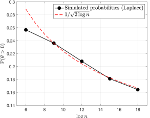
In particular, for the Laplace distribution , and the convergence rate is .
4.3 Likelihood-ratio statistic
The likelihood-ratio statistic for testing is
Our goal here is to establish the asymptotic null distribution, particularly the conditional distribution given .
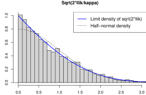
The conventional arguments based on Taylor expansion (see Appendices A.1 and A.3 of Brazzale and Mameli, 2024) do not apply because the th log-likelihood derivative at zero is equal to , where belongs to the domain of attraction of the stable law with index . The first derivative does not have a finite variance, so there is no concept of Fisher information. Higher-order derivatives do not have an expectation, and are strongly dependent. Nevertheless, one series of simulations shown in the right panel of Fig. 4 suggests that the asymptotic null distribution given is close to , where the Bartlett factor tends to one. This section offers an explanation and a derivation of the correct limit distribution, which is not in the setting of Theorem 3.1.
Theorem 4.1.
Let be independent standard Gaussian, let be in the domain of attraction of the Cauchy law, and let be the cumulative distribution function whose th quantile is
| (19) |
Then, the conditional limit distribution of the likelihood-ratio statistic is
Remark 4.1.
The limit distribution is not dissimilar to . Both densities have the same -singularity at the origin. The first four cumulants of are 1, 2, 8, and 96, while those of are 1, 7/3, 32/3, and 3194/45. However, for , the log density of has a Taylor expansion
which is essentially linear for , while the corresponding half-normal log density is exactly quadratic and negative at zero. The difference between and the degree-4 Taylor approximation is less than 1% for .
Proof.
For notational simplicity we set , so that is in the Cauchy domain of attraction with zero mean, and Theorem 3.2 applies. Given , we construct an approximation for and its derivatives , where
Both and are conditionally , while the conditional distribution of is asymptotically the same as the unconditional distribution of . Since is in the domain of attraction of the stable law with index , the scaling constant is , and we have
It follows that for . Thus, the log likelihood may be approximated locally by substituting for , giving
| (20) |
with for .
Theorem 3.2 shows that is less than one with high probability for large , in which case has a maximum at . In that case , and the approximate likelihood-ratio statistic
| (21) |
is a monotone function of . Theorem 3.2 also shows that the limit distribution of given is uniform on , implying that in the limit. ∎
Figure 4 shows a histogram of and the Bartlett-adjusted likelihood ratio statistic using the exact likelihood and the exact maximum in the Gauss-Cauchy mixture model restricted to 2000 out of 74058 samples for which . For this model, is the slow-variation function, and . For the simulation, , is the sample average, and in 31 cases. The sample cumulant ratios and for compared with are 1.160 and 1.346, which are surprisingly close to the theoretical limit values and respectively. The new limit density is shown on the same square-root scale, together with the half-normal density for comparison. While the difference between the two distributions is not large, the histogram clearly favours . A standard 20-bin -test gives for the distribution, and for .
Analogous simulations for the Gauss-Laplace mixture give virtually identical results for the likelihood-ratio statistic, though with . However, the fraction of -values greater than one was 249/2000, or 12%, consistent with a convergence rate. The argument used in the proof of Theorem 4.1 suggests that the rate of convergence of to might be or perhaps , but the simulations suggest a faster rate, particularly after Bartlett correction.
The local approximation (20) and ensuing argument is valid for any iid problem with a boundary at zero provided that the log likelihood derivative is a sum of zero mean random variables in the Cauchy domain of attraction. However the adequacy of the approximation (20) depends on the behaviour of higher derivatives, which is context specific.
4.4 Predictive activity rate
Given an estimate of , the fitted or predictive activity rate for unit is
| (22) |
and the complement is called the (fitted) local false discovery rate. If , the fitted activity rate is zero for every unit, and the false-discovery rate is one: every unit is deemed to have a null or negligible signal. Given , the maximum predicted activity rate is
where is the maximum absolute sample value.
Proof.
Since is uniformly distributed on in the large-sample limit for , the minimum fitted local false discovery rate is , whose conditional null distribution is also uniform on in the large-sample limit. Given , with probability tending to 1. In the rare event that , the conditional probability that some unit is declared active or non-null at level is equal to in the large-sample limit,
4.5 Wald and Rao statistics
The conventional Wald and Rao statistics for testing are
where is the log likelihood function and is the Fisher information. Technically speaking, the Rao statistic does not exist in the mixture setting because is not finite. For present purposes, however, we substitute for in both.
Given , the approximate likelihood in section 4.3 implies
where . It follows that the modified Wald and Rao statistics are
In other words, the two statistics are conditionally equivalent given , both uniformly distributed on . The squared statistics are not approximately the same as the likelihood-ratio statistic, although all three are asymptotically equivalent in the sense that each is a monotone function of . Conventional standard normal approximations are incorrect.
Reproducibility.
We provide code to reproduce Figures 1, 2 and 4 on Github, under the repository: https://github.com/dan-xiang/dan-xiang.github.io/tree/master/non-standard-boundary-paper.
Appendices
Appendix I: De Bruijn group
The de Bruijn group is the set of slowly-varying functions together with the non-commutative binary operation . To see that this is an associative function , observe that
Associativity implies that the triple product is well-defined by the pairwise products. The identity element: is the unit constant function. If it exists, the inverse is a slowly-varying function such that for all . Since slow variation is a characterization of the limiting behaviour for large , it says little about the behaviour for general beyond continuity or measurability. Thus, the existence of an inverse is not guaranteed. Nevertheless, the following theorem suffices for present purposes.
Theorem .2 (de Bruijn 1959).
To each there corresponds a function , satisfying for all sufficiently large.
Proof.
Theorem 1.5.13 of Bingham, Goldie and Teugels (1987) proves existence in the sense of equivalence. Theorem 1.8.9 proves existence as stated above, i.e., for all sufficiently large. ∎
Although the product is ultimately monotone, it is not necessarily monotone for small . Thus, contains functions for which no group inverse exists (as a function ). The theorem states that an asymptotic inverse exists, which implies that the set of equivalence classes is a group. For the most part, it is the group of equivalence classes that is of interest here. However, we always work with a representative element.
Appendix II: Approximation of the sine-integral
Let be the cumulative function of a finite-mean distribution on the positive real line, and let be the right-tail probability. Since uniformly in as , the derivative (with respect to at ) tends to zero. Hence
We first split the integrand into two parts, , and split the range into disjoint intervals and , where is large. Then
| (23) |
where is the mean. The first integrand is bounded by for , so the contribution from the interval is bounded by
Appendix III: Calculation of the asymmetric Cauchy density
By the Fourier inversion formula of the characteristic function for and , the asymmetric Cauchy density in Fig. 1 is
Substitute , which is increasing over . As becomes large, the integral over the interval is exponentially small in , and may be ignored:
where is the inverse map for the substitution. From here on, we ignore the exponentially small remainder term. It is easy to check that
from which it follows that the integral is
where means a term that goes to zero as . Then the above is
Now using , the above expression becomes
The first term gives
The second term is
since . Finally, note that the above term is equal to
To summarize, we have shown that for large ,
which implies for the right tail. For ,
so the argument above implies that as ,
and .
Appendix IV: Proof of Proposition 4.1
Suppose , with symmetric about zero with density function having exponential index in the sense that:
for some slowly varying function . Then the Gaussian convolution has exponential tail index .
Proof.
Let and . The convolution density is
for some slowly varying . Since , we have as , so that
for sufficiently large. It follows that, over the range of the integral, we have
This implies is bounded by
for some constant . Now since , the above reduces to
for some slowly varying function . The formula implies
Finally, implies
for some slowly varying , from which it follows that
A similar argument yields for some slowly varying , which implies
so that is also slowly varying, completing the proof.
∎
Acknowledgement
P. McC is grateful to Titus Hilberdink for advice concerning regular-variation integrals and for pointing out the connection with de Bruijn conjugates.
References
- [1] Bingham, N. H, Goldie, C. M. and Teugels, J. L. (1987). Regular Variation. Cambridge University Press, Cambridge, UK.
- [2] Brazzale, A. R. and Mameli, V. (2024). Likelihood asymptotics in nonregular settings: a review with emphasis on the likelihood ratio. Statist. Sci., 39, 322–345.
- [3] de Bruijn, N. G. (1959). Pairs of slowly oscillating functions occurring in asymptotic problems concerning the Laplace transform. Nieuw Arch. Wisk., 7, 20–26.
- [4] Chernoff, H. (1954). On the distribution of the likelihood ratio. Ann. Math. Statist., 25, 573–578.
- [5] Chow, T. L. and Teugels, J. L. (1979) The sum and the maximum of i.i.d. random variables. In Proceedings of the Second Prague Symposium on Asymptotic Statistics, Petr Mandl and Marie Hušková, Editors, 81–92. North Holland Publishing Company.
- [6] Efron, B., Tibshirani, R., Storey, J. D., and Tusher, V. (2001). Empirical Bayes analysis of a microarray experiment. J. Amer. Statist. Assoc., 96, 1151–1160.
- [7] Efron, B. (2012). Large-scale inference: empirical Bayes methods for estimation, testing, and prediction (Vol. 1). Cambridge University Press.
- [8] Geyer, C. J. (1994). On the asymptotics of constrained M-estimation. Ann. Statist., 22, 1993–2010.
- [9] Ghosh, J. K. and Sen, P. K. (1985). On the asymptotic performance of the log likelihood ratio statistic for the mixture model and related results. In Proceeding of the Berkeley Conference in honour of Jerzy Neyman and Jack Kiefer, 789–806.
- [10] Gnedenko, B. V and Kolmogorov, A. N. (1954). Limit Distributions for Sums of Independent Random Variables. Translated from the Russian and annotated by K. L. Chung; with an appendix by J. L. Doob. Addison-Wesley Pub. Co., Cambridge, Massachusetts.
- [11] Patra, R. K. and Sen, B. (2016). Estimation of a Two-component Mixture Model with Applications to Multiple Testing. J. R. Statist. Soc. B, 78, 869–893.
- [12] Self, S. G. and Liang, K-Y. (1987). Asymptotic properties of maximum likelihood estimators and likelihood ratio tests under nonstandard conditions. J. Amer. Statist. Assoc., 82, 605–610.
- [13] Vu, H. T. V. and Zhou, S. (1997). Generalization of likelihood ratio tests under nonstandard conditions. Ann. Statist., 22, 1993–2010.
- [14] Zolotarev, V. M. (1986). One-dimensional Stable Distributions. American Mathematical Society, Providence.