Machine Learning for predicting chaotic systems

Abstract

Predicting chaotic dynamical systems is critical in many scientific fields such as weather prediction, but challenging due to the characterising sensitive dependence on initial conditions. Traditional modeling approaches require extensive domain knowledge, often leading to a shift towards data-driven methods using machine learning. However, existing research provides inconclusive results on which machine learning methods are best suited for predicting chaotic systems. In this paper, we compare different lightweight and heavyweight machine learning architectures using extensive existing databases, as well as a newly introduced one that allows for uncertainty quantification in the benchmark results. We perform hyperparameter tuning based on computational cost and introduce a novel error metric, the cumulative maximum error, which combines several desirable properties of traditional metrics, taylored for chaotic systems. Our results show that well-tuned simple methods, as well as untuned baseline methods, often outperform state-of-the-art deep learning models, but their performance can vary significantly with different experimental setups. These findings underscore the importance of matching prediction methods to data characteristics and available computational resources.

1 Introduction

In many scientific disciplines, predicting the behavior of dynamical systems is a crucial objective. Systems such as the climate, chemical reactions, and mechanical processes often exhibit chaotic behavior [Ott02, Str24]. Chaotic systems are characterized by their sensitive dependence on initial conditions, making them notoriously difficult to predict and presenting a significant challenge for researchers studying them.

A traditional approach to addressing this problem involves using domain knowledge to model the dynamical system. However, this approach requires detailed understanding of the specific system, which may not be available. In recent years, system-agnostic, data-driven approaches have emerged as a viable alternative. These methods, which leverage techniques from statistics and machine learning, are trained on observational data to predict the future behavior of the system.

These predictive methods range from relatively simple and computationally inexpensive, such as fitting polynomials, to highly sophisticated models that utilize complex neural network architectures, demanding significant computational power for training. To evaluate these approaches, various comparison studies have been conducted.

For instance, [Han+21] focuses on complex machine learning models with mostly classical neural network architectures. They do not include the sophisticated transformer model [Vas+17], which has gained popularity due to its effectiveness for large language models. Such models are surveyed in [Wen+22], where different variants of transformer models for time series forecasting are reviewed. Remarkably, [Zen+23] demonstrate how simple linear methods can outperform these complex models. Additionally, [Vla+20] compare reservoir computers (RCs) and recurrent neural networks (RNNs), favoring RNNs, whereas [SFC22] conducts a similar comparison, adding further machine learning methods and concluding that RCs are preferable.

Previous studies typically compare methods on a limited number of systems. However, [Gil21, Gil23] emphasize the use of extensive datasets and benchmarks to evaluate the performance of different methods. They introduce a database of more than 130 different chaotic dynamical systems and, in their comparison study, find that the sophisticated NBEATS method [Ore+19] performs best. Hyperparameter tuning in this study is minimal, despite its importance for algorithm performance.

All in all, there is no consensus in the literature on which method should be preferred. Even the distinction between lightweight and heavyweight methods is not clear. Apart from using only a few systems (and often different data in each study), lacking robustness of comparisons may stem from an inherent randomness in the evaluations. The results of the error metrics used may vary when different initial conditions are applied. If experiments are repeated only a few times with randomly drawn initial conditions, the results may still not be robust. If there is only one repetition, then uncertainty cannot even be judged.

With this work, we aim to address different shortcomings of previous studies. We compare various lightweight and heavyweight algorithms, including simple statistical methods that have shown promising performance but have received limited attention [RH17]. We tune hyperparameters guided by the computational cost of each algorithm, allocating more resources for lightweight methods and less for heavyweight ones.

As one source of (synthetic) observational data, we take the Dysts database of [Gil21] to have a wide range of chaotic systems and to allow for direct comparison with the results in [Gil23]. Additionally, we introduce a new database, DeebLorenz, which encompasses three variations of the well-known Lorenz63 system [Lor63], allowing for an easy comparison with other studies. It includes 100 repetitions of simulated observational data for each system to increase robustness of results and to allow uncertainty quantification. The database also features a nonparametric version of Lorenz63 to assess the performance of polynomial-based fitting algorithms on non-polynomial targets. Different observation schemes are used for each system to examine the impact of noise and time step intervals on performance. Furthermore, we propose a new error metric for forecasting task on dynamical systems, the cumulative maximal error ($\mathsf{CME}$). It combines the benefits of integrated error based methods (as used in, e.g., [Gil23, God+21]) and the valid time $t_{\mathsf{valid}}$, e.g., [Ren+09, Pat+18].

Our simulation study demonstrates significantly better performance of various tuned and untuned simple methods compared to complex machine learning models. Additionally, we find that the relative performance of methods is highly dependent on the experimental setup, though some trends, such as the strong performance of simple methods, remain consistent. Notably, introducing random time steps between consecutive observations dramatically alters performance, with a Gaussian process-based method [RW05, Hei+18], which ranks mid-tier under constant time steps, outperforming all other methods.

The remaining parts of the paper are structured as follows: Section 2 describes the databases, the forecasting task, the methods compared, the $\mathsf{CME}$ error metric, and the hyperparameter tuning. The results and key insights of the simulation study are described in Section 3. Appendix A provides additional details on the databases, followed by a discussion of the estimation methods in Appendix B. Finally, tables and plots detailing the simulation study results are available in Appendix C.

2 Methodology

2.1 Data

We are using two different databases: DeebLorenz, a database created specifically for this study, and the Dysts database from [Gil21]. An overview of their structure is given in Figure 1, and further details are described below.

Both databases consist of solutions $u\colon\mathbb{R}\to\mathbb{R}^{d}$ of autonomous, first-order ordinary differential equations (ODEs), i.e., $\dot{u}(t)=f(u(t))$, where $\dot{u}$ is the derivative of $u$ and $f\colon\mathbb{R}^{d}\to\mathbb{R}^{d}$ is the model function describing the dynamics of the system. All considered systems are chaotic, i.e., they show a sensitive dependence on initial conditions, an aperiodic long-term behavior, and a fractal structure in the state space [Ott02, Str24].

Figure 1: Visual overview over the databases used in this study.

2.1.1 DeebLorenz

All three systems considered in DeebLorenz are related to the Lorenz63 system [Lor63], in which $f\colon\mathbb{R}^{3}\to\mathbb{R}^{3}$ is a sparse polynomial of degree 2 with 3 parameters. In Lorenz63std, the parameters are fixed to their default values used in the literature. In Lorenz63random the parameters are drawn randomly. In LorenzNonparam the parameters change with the state using a random nonparametric function drawn from a Gaussian process.

The data is generated under different observation schemes: Initial conditions $u(0)$ are drawn randomly from the attractor of the system. For times $t_{1},\dots,t_{n}\in[0,T]$, $T\in\mathbb{R}_{>0}$, the state $u(t_{i})$ is recorded either directly as $Y_{i}=u(t_{i})$ or with random measurement error $\varepsilon_{i}$, i.e., $Y_{i}=u(t_{i})+\varepsilon_{i}$. The observation times $t_{i}$ either have a constant timestep so that $t_{i}=iT/n$ or timesteps are drawn randomly from an exponential distribution $t_{i+1}-t_{i}\sim\mathsf{Exp}(\lambda)$. All combinations of these timestep and measurement options make up the four different observation schemes for DeebLorenz.

For each combination of the three systems and four observation schemes, the generation of the data training data $(t_{i},Y_{i})_{i=1,\dots,n}$, $t_{i}\in[0,T]$ with $n=10^{4}$ and testing data $(t_{j},u(t_{j}))_{j=n+1,\dots,n+m}$, $t_{j}\in[T,T+S]$, $S\in\mathbb{R}_{>0}$, with $m=10^{3}$ is repeated with different random seeds to create a tuning set (10 repetitions) and an evaluation set (100 repetitions). A more detailed description can be found in Section A.2.

2.1.2 Dysts

The Dysts dataset consists of 133 chaotic systems with dimensions between 3 and 10, observed with constant timesteps, i.e., $t_{i}=iT/n$, and two different noise settings: one without noise $Y_{i}=u(t_{i})$, $\dot{u}(t)=f(u(t))$; the other with system noise, i.e., $Y_{i}=u(t_{i})$ with

$$\mathrm{d}u(t)=f(u(t))\mathrm{d}t+\sigma\mathrm{d}B(t)\,,$$ (1)

where $B(t)$ is a standard Brownian motion and $\sigma\in\mathbb{R}_{>0}$ is the scale of the noise. For both observation schemes, data are available in a tune set and an evaluation set, which each consist of one repetition of generated training data $(t_{i},Y_{i})_{i=1,\dots,n}$ with $n=10^{3}$ and testing data $(t_{j},u(t_{j}))_{j=n+1,\dots,n+m}$ with $m=200$ for each of the 133 systems.

2.2 Task and Evaluation

For all datasets, systems, and observation schemes, we impose the following task: Given the observations of the past, $(t_{i},Y_{i})_{i=1,\dots,n}$ in the time interval $t_{i}\in[0,T]$ (training time), and the true current state $u(T)$, predict the future states $u(t_{j})$ at given times $t_{j}\in[T,T+S]$ (testing time) for $j=1,\dots,m$.

We apply and compare different statistical and machine learning methods on this task. The methods are described below in Section 2.3. For a given method, we first tune its hyperparameters on the tuning data for each system individually. Then we train the method on the training data of the evaluation set and create the predictions $\hat{u}(t_{j})$ for the testing time. The predictions are compared with the ground truth $u(t_{j})$ using different metrics.

We calculate the following three metrics for comparing an estimate $\hat{u}(t)$ with the ground truth $u(t)$ in the testing time $t\in[T,T+S]$:

• The valid time $t_{\mathsf{valid}}$, e.g., [Ren+09, Pat+18], for a given threshold $\kappa\in\mathbb{R}_{\geq 0}$ is defined as the duration such that the normalized error stays below $\kappa$, i.e.,

  $$t_{\mathsf{valid}}(\hat{u},u):=\inf\left\{t\in[T,T+S]\,\kern-1.2pt\mathopen{}\left|\vphantom{t\in[T,T+S]}\,\frac{\left\|\hat{u}(t)-u(t)\right\|_{2}}{\mathsf{sd}(u)}>\kappa\right.\mathclose{}\kern-1.2pt\right\}-T$$ (2)

  where $\|\cdot\|_{2}$ denotes the Euclidean norm and $\mathsf{sd}(u)$ is the standard deviation of $u$ in the interval $[T,T+S]$, i.e.,

  $$\mathsf{sd}(u):=\sqrt{\frac{1}{S}\int_{T}^{T+S}\left\|u(t)-\mu(u)\right\|_{2}^{2}\mathrm{d}t}\,,\qquad\mu(u):=\frac{1}{S}\int_{T}^{T+S}u(t)\mathrm{d}t\,.$$ (3)

  If the threshold is not reached, we set $t_{\mathsf{valid}}=S$. In our evaluation, we set the threshold as $\kappa=0.4$. Note that the normalization, i.e., division by $\mathsf{sd}(u)$, is often done differently in the literature: [Ren+09] do not integrate but normalize by $\|u(t)\|_{2}$, and [Pat+18] do not remove the mean $\mu(u)$ in (3).

• The symmetric mean absolute percent error $\mathsf{sMAPE}$, e.g., [Gil23, God+21], is defined as

  $$\mathsf{sMAPE}(\hat{u},u):=\frac{2\cdot 100\%}{S}\int_{T}^{T+S}\frac{\left\|\hat{u}(t)-u(t)\right\|_{2}}{\left\|\hat{u}(t)\right\|_{2}+\left\|{u(t)}\right\|_{2}}\mathrm{d}t\,.$$ (4)

• For this study, we design a new error metric, the cumulative maximum error $\mathsf{CME}$. It is defined as

  $$\mathsf{CME}(\hat{u},u):=\frac{1}{S}\int_{T}^{T+S}\max_{s\in[T,t]}\min\!\left(1,\,\frac{\left\|\hat{u}(s)-u(s)\right\|_{2}}{\mathsf{sd}(u)}\right)\mathrm{d}t$$ (5)

  with $\mathsf{sd}$ as in (3). It combines the advantages of $t_{\mathsf{valid}}$ and $\mathsf{sMAPE}$, see Section 2.4 for details.

In practice, the canonical discrete-time versions of these metrics are applied, i.e., integrals are replaced by a suitable sum.

2.3 Estimation Methods

We apply a wide range of different methods. Additionally, for the noisefree version of the Dysts dataset, we also include the methods evaluated in [Gil23] in our benchmark (pre-calculated predictions are not available for the noisy version). Names of these reference methods start with an underscore, e.g., _NBEAT. In this section, we give a broad descriptions for the methods specifically executed for this study. A more detailed description can be found in Appendix B.

The methods can be separated into propagators, solution smoothers, and other methods that do not belong to either of these two groups.

Let us start with the last category, which also contains our baselines:

• ConstM (also called climatology): The prediction $\hat{u}(t)$ is the constant mean of the observed states, i.e., $\frac{1}{n}\sum_{i=1}^{n}Y_{i}$.

• ConstL (also called persistence): In our prediction task, the noisefree true state at time $T$ is always available to the methods, even in an observation scheme with noise. For this method, we set $\hat{u}(t):=u(T)$ for all $t$.

• Analog: For the method of the analog, we find the observed state $Y_{i_{0}}$ with the closest Euclidean distance to $u(T)$ and predict $\hat{u}(T+k\Delta\!t)=Y_{i_{0}+k}$ or a linear interpolation thereof if timesteps are not constant.

• Node: In the neural ODE [Che+18], a neural network $f_{\theta}$ is fitted to the data such that solving the ODE $\dot{\hat{u}}(t)=f_{\theta}(\hat{u}(t))$ minimizes the error $\|\hat{u}(t_{i})-Y_{i}\|_{2}$.

The methods ConstM, ConstL, and Analog can be treated as trivial baselines as no fitting or learning is required. Next, we consider the group of propagators: For these methods, the basic idea is to find an estimate for the so-called propagator map

$$\mathcal{P}_{\Delta\!t}\colon u(t)\mapsto u(t+\Delta\!t)\qquad\text{or equivalently}\qquad\mathcal{P}_{\Delta\!t}\colon\mathbb{R}^{d}\to\mathbb{R}^{d},\,x\mapsto u_{x}(\Delta\!t)\,,$$ (6)

where $u_{x}$ solves the initial value problem $\dot{u}_{x}(t)=f(u_{x}(t))$, $u_{x}(0)=x$. This task can be formulated as a regression problem on the data $(Y_{i},Y_{i+1})_{i=1,\dots,n-1}$ assuming constant timesteps $t_{i+1}-t_{i}=\Delta\!t$. After the propagator is estimated, recursive application yields the predictions

$$\hat{u}(T+k\Delta\!t)=\underbrace{\mathcal{P}_{\Delta\!t}(\dots\mathcal{P}_{\Delta\!t}(}_{k\text{ times}}u(T))\dots)\,.$$ (7)

All methods listed next are variations on this basic idea. Several of them come in four flavors marked by * below and the suffix S, D, ST, or DT in their name: S indicates (6) as a target, whereas D means that difference quotient

$$x\mapsto\frac{u_{x}(\Delta\!t)-x}{\Delta\!t}$$ (8)

is estimated and the prediction formula is adapted suitably. If T is part of the suffix, the timestep $t_{i+1}-t_{i}$ is available for the method as an input for the prediction of $u(t_{i+1})$.

• PgGp*, PgNet*, PgLl*: Fit $\mathcal{P}_{\Delta\!t}$ with a Gaussian process [RW05], a feed-forward neural network [RHW86], or a local linear estimator [RW94], respectively.

• Lin*: The propagator $\mathcal{P}_{\Delta\!t}$ is estimated via ridge regression [Has+09, chapter 3.4.1] using polynomial features. For a prediction of $u(t_{i+1})$, state values at times $t_{i-sk}$, $k=0,\dots,K$ for a fixed $s\in\mathbb{N}$ are available as inputs to the polynomial features. This method is also called a nonlinear vector autoregressive model [Gau+21].

• LinPo2, LinPo4: Tuning-free versions of LinD with linear regression (ridge penalty parameter equal to $0$), without past states as predictors ($K=0$), and with the polynomial degree fixed to $2$ and $4$, respectively.

• RaFe*: For Random Features [RR08], features are created from the predictors (the current state variables) by applying a once randomly created and untrained neural network. Then ridge regression [Has+09, chapter 3.4.1] is applied to estimate the mapping from features to targets (the next state).

• Esn*: The Echo State Network [Jae01], also referred to as a reservoir computer, is similar to Random Features, but features of the previous timestep are also inputs for the feature calculation of the current timestep.

• Trafo: A transformer network [Vas+17] that uses attention layers to compute the next state from a sequence of previous states is applied.

Finally, the solutions smoothers [RH17, chapter 8] work in three steps: First estimate $u(t)$ in the observation time $[0,T]$ with a regression estimator $\tilde{u}(t)$. Then view the data $(\tilde{u}(t),\dot{\tilde{u}}(t))_{t\in[0,T]}$ as observations of $(x,f(x))$ and use a second regression estimator to obtain an estimate $\hat{f}$. Lastly, solve the ODE $\dot{\hat{u}}(t)=\hat{f}(\hat{u}(t))$ on the time interval $[T,T+S]$ with initial conditions $\hat{u}(T)=u(T)$.

• PwNn: The observed solution is interpolated with a piece-wise linear function $\tilde{u}$, from which $\hat{f}$ is generated by a nearest neighbor interpolation.

• SpNn: As PwNn, but $\tilde{u}$ is cubic spline interpolation [For+77].

• LlNn: As PwNn, but $\tilde{u}$ is local linear regression [Fan93].

• SpPo: As SpNn, but $\hat{f}$ is ridge regression [Has+09, chapter 3.4.1] with polynomial features.

• SpPo2, SpPo4: Tuning-free version of SpPo with linear regression (ridge penalty parameter equal to $0$) and with fixed polynomial degree 2 and 4, respectively.

• SpGp: As SpNn, but $\hat{f}$ is Gaussian process regression [RW05].

• GpGpI, GpGpR: As SpGp, but $\tilde{u}$ is also Gaussian process regression. The two methods differ only in the hyperparmeter domain: GpGpI tends to be closer to interpolation, whereas GpGpR leans more towards regression. The methods are similar to the one proposed in [Hei+18].

• SINDy, SINDyN: As SpPo without $L_{2}$-penalty, but sparsity is enforced for the polynomial $\hat{f}$ via thresholding [BPK16]. As for all other methods, data normalization is applied before the actual estimation method for SINDyN. Only for SINDy it is turned off to not destroy potential sparsity in the original data. The name SINDy is short for Sparse Identification of Nonlinear Dynamics.

2.4 Cumulative Maximum Error – CME

Although different error metrics are calculated to evaluate the results of this simulation study, we focus on the $\mathsf{CME}$ (5). If time is discrete, (5) becomes

$$\mathsf{CME}_{m}(\hat{u},u):=\frac{1}{m}\sum_{j=1}^{m}\max_{k=1,\dots,j}\min\!\left(1,\,\frac{\left\|\hat{u}(t_{k})-u(t_{k})\right\|_{2}}{\mathsf{sd}_{m}(u)}\right)\,.$$ (9)

where

$$\mathsf{sd}_{m}(u):=\sqrt{\frac{1}{m}\sum_{j=1}^{m}\left\|u(t_{j})-\mu_{m}(u)\right\|_{2}^{2}}\,,\qquad\mu_{m}(u):=\frac{1}{m}\sum_{j=1}^{m}u(t_{j})\,.$$ (10)

Similar to the $\mathsf{sMAPE}$, errors are integrated over time, and similar to $t_{\mathsf{valid}}$, the future evolution of the predictions is discarded after a threshold is reached. The $\mathsf{CME}$ has many desirable properties:

1. It is translation and scale invariant, in contrast to $\mathsf{sMAPE}$ and the version of the valid time used in [Ren+09, Pat+18], but similar to our definition of $t_{\mathsf{valid}}$. This is desirable as every ODE system can be modified to create any translation and scaling of its solutions. Thus, the evaluation of an estimator $\hat{u}$ should not depend on the location and scale of the system.

2. We focus on a task that involves evaluating the precise state within a near-future time interval, as in weather forecasting. In contrast, one could also consider a task where the long-term behavior of the prediction should resemble the ground truth, without emphasizing the error at any single point in time, as in climate modeling. For the former task, predictive power deteriorates quickly over time due to the chaotic nature of the systems considered. Therefore, if the prediction interval $[T,T+S]$ is long, we are primarily interested in the early times when accurate prediction is possible. Accurate predictions at the beginning of the interval should not be discounted by divergence at the end. This requirement is captured by $\mathsf{CME}$ and, to some extent, by $t_{\mathsf{valid}}$, but not by $\mathsf{sMAPE}$.

3. The value of the $\mathsf{CME}$ is always between 0 and 1, where 0 is only achieved by perfect prediction. In contrast, the scale of $t_{\mathsf{valid}}$ depends strongly on the system’s time scale and the best value $t_{\mathsf{valid}}=S$ can be achieved for imperfect predictions.

4. Dealing with missing values when calculating the $\mathsf{CME}$ is canonical: If $\hat{u}(t)$ is not available for some $t$, we set the value of the minimum in (5) to $1$. Consistently, if all of the prediction is missing, we set the $\mathsf{CME}$ to $1$.

5. The $\mathsf{CME}$ is parameter-free in contrast to $t_{\mathsf{valid}}$, where the threshold $\kappa$ has to be specified.

6. If time is discrete, $t_{\mathsf{valid}}$ can only attain a finite number of values. In contrast, for all values in $[0,1]$ there is a prediction $\hat{u}$ such that $\mathsf{CME}_{m}(\hat{u},u)$ attains this value. Furthermore, $\hat{u}_{1}$ and $\hat{u}_{2}$ may have the same $t_{\mathsf{valid}}$, but $\|\hat{u}_{1}(t)-u(t)\|_{2}<\|\hat{u}_{2}(t)-u(t)\|_{2}$ for all $t\in[T,T+t_{\mathsf{valid}})$. If time is discrete, we can even have $\|\hat{u}_{1}(t)-u(t)\|_{2}<\|\hat{u}_{2}(t)-u(t)\|_{2}$ for all $t\in[T,T+S]$ while $t_{\mathsf{valid}}(\hat{u}_{1},u)=t_{\mathsf{valid}}(\hat{u}_{2},u)$. This cannot happen with $\mathsf{CME}$: If $\|\hat{u}_{1}(t)-u(t)\|_{2}<\|\hat{u}_{2}(t)-u(t)\|_{2}$ for all $t\in[T,t^{*}]$ for some $t^{*}>T$ and $\|\hat{u}_{1}(t)-u(t)\|_{2}\leq\|\hat{u}_{2}(t)-u(t)\|_{2}$ for all $t\in[t^{*},T+S]$, we have $\mathsf{CME}(\hat{u}_{1},u)<\mathsf{CME}(\hat{u}_{2},u)$.

Let us also describe potential drawbacks of the $\mathsf{CME}$.

1. The $\mathsf{CME}$ is not symmetric, $\mathsf{CME}(\hat{u},u)\neq\mathsf{CME}(u,\hat{u})$ in general, in contrast to $\mathsf{sMAPE}$. But in our use case, the relationship between its two arguments $\hat{u}$ and $u$ is also not symmetric. Thus, there does not seem to be a benefit to symmetry.

2. If $u$ is constant, then $\mathsf{sd}(u)=0$ and (5) is not valid. In this case, a reasonable definition is to set $\mathsf{CME}$ to $1$ for all $\hat{u}$ except the perfect prediction $\hat{u}=u$ in which case $0$ is the appropriate value. Note that $t_{\mathsf{valid}}$ (and to some extent $\mathsf{sMAPE}$) also suffers from this division by zero-problem.

3. If a prediction gets far away from $u(t)$ but recovers at a later point in time, the recovery is not accredited in $\mathsf{CME}$. As future states in our dynamical systems are independent of the past given the present (Markov property), this is a lesser issue. But note that the same distance $\delta=\|\hat{u}(t_{0})-u(t_{0})\|_{2}$ can translate to different future predictability at times $t>t_{0}$ for different states $u(t_{0})=x_{1}$ or $u(t_{0})=x_{2}$, $x_{1}\neq x_{2}$. I.e., we can have

   $$\left\|u_{x_{1}}(t)-u_{x_{1}^{\prime}}(t)\right\|_{2}\neq\left\|u_{x_{2}}(t)-u_{x_{2}^{\prime}}(t)\right\|_{2}$$ (11)

   for $t>t_{0}$ even if $\|x_{1}-x_{1}^{\prime}\|_{2}=\|x_{2}-x_{2}^{\prime}\|_{2}$.

4. On one hand, the value $1$ is the $\min$-term of (5) could be replaced by a threshold parameter $\kappa$ as in $t_{\mathsf{valid}}$, removing the advantage of being parameter-free for the $\mathsf{CME}$. On the other hand, $\kappa=1$ is a natural choice for the $\mathsf{CME}$ (in contrast to $t_{\mathsf{valid}}$), as the trivial baseline ConstM, $\hat{u}(t)=\sum_{i=1}^{n}Y_{i}$, achieves $\left\|\hat{u}(s)-u(s)\right\|_{2}/\mathsf{sd}(u)=1$ on average in the noisefree setting. Furthermore, for every constant prediction there is a finite time point $s_{0}$ such that $\left\|\hat{u}(s)-u(s)\right\|_{2}/\mathsf{sd}(u)\geq\kappa$ for $\kappa=1$ and $\kappa=1$ is largest value with this property.

5. The value of the $\mathsf{CME}$ depends on the testing duration $S$ (similar to $\mathsf{sMAPE}$, but in contrast to $t_{\mathsf{valid}}$). This could be mitigated by setting $S=\infty$ and multiplying the integrand in (5) by a weighting function $w(t-T)$, e.g., $w(\tau)=\exp(-\alpha\tau)$, but this introduces a new parameter choice $\alpha\in\mathbb{R}_{>0}$. To make the weighting choice-free on time-scale adaptive, $\alpha$ needs to be set depending on $u$, e.g., to the inverse correlation time.

2.5 Hyperparameter Tuning

Each pair of a dynamical system and an observation scheme comes as a tune dataset and an evaluation dataset. For hyperparameter tuning only the tune dataset is used. Each such dataset consists of $1$ (Dysts) or $10$ (DeebLorenz) repetitions. Each repetition consists of training and testing data.

For a given method $\hat{u}_{\mathbf{a}}$ with hyperparameters $\mathbf{a}$, we train it, predict, and calculate the $\mathsf{CME}$ for different $\mathbf{a}$. Let us denote $\mathsf{CME}(\mathbf{a})$ the average $\mathsf{CME}$ of all repetitions and the best hyperparameters among the tested ones as $\mathbf{a}^{*}=\operatorname*{arg\,min}_{\mathbf{a}}\mathsf{CME}(\mathbf{a})$. Then $\hat{u}_{\mathbf{a}^{*}}$ is applied to the evaluation dataset for the finial results presented in Section 3. See Appendix B for a description of the tuned hyperparameters for each method.

To decide which hyperparameters $\mathbf{a}$ to evaluate, we follow a local grid search procedure: For a given estimation method, decide on which parameters should be tuned $\mathbf{a}=(a_{1},\dots,a_{\ell})$. Each parameter $a_{j}$ has a domain of possible values $\mathcal{A}_{j}$. Furthermore, it can be categorical or scalar. For categorical parameters, decide whether they are persistent (always evaluate all options) or yielding (only evaluate best). For scalar parameters, decide on a linear or exponential scale and a stepsize $s_{j}\in\mathbb{R}_{>0}$. Define the sets of initial values $A_{0,1},\dots,A_{0,\ell}$ for each hyperparameter. Now for step $k\in\mathbb{N}_{0}$ in the optimization procedure, evaluate all elements of the grid of hyperparameters $(a_{1},\dots,a_{\ell})\in A_{k,1}\times\dots\times A_{k,\ell}$ that have not been evaluated before. If there are none, stop the search. Denote the best hyperparameter combination evaluated so far as $(a_{k,1}^{*},\dots,a_{k,\ell}^{*})$. Generate $A_{k+1,j}$ from $a_{k,j}^{*}$ as follows: If the $j$-th variable is categorical, set $A_{k+1,j}=A_{0,j}$ for persistent parameters and $A_{k+1,j}=\{a_{k,j}^{*}\}$ for yielding ones. If the $j$-th variable is scalar, set $A_{k+1,j}=\{a_{k,j}^{*}-s_{j},a_{k,j}^{*},a_{k,j}^{*}+s_{j}\}\cap\mathcal{A}_{j}$ if it has a linear scale and $A_{k+1,j}=\{a_{k,j}^{*}/s_{j},a_{k,j}^{*},s_{j}a_{k,j}^{*}\}\cap\mathcal{A}_{j}$ if the scale is exponential.

The local grid search finds locally optimal hyperparameter combinations with a reasonable amount of evaluations. In this study, the algorithm is applied to $\ell\leq 4$ hyperparameters to limit the computational costs. We tune more parameters in case of methods with low computational demand and limit to one categorical variable without search for the most expensive methods. See Table 34 and Table 36 for the computational cost of hyperparameter tuning. By this, we try to make the comparison more fair regarding total computational costs. The resulting total compute time can still be rather different between methods. This is partially due to the adaptive nature of the local grid search algorithm (i.e., the total number of predictions cannot be known beforehand) and partially due to the lack of meaningful tunable hyperparameters for some methods (in particular for very simple method that typically have low computational costs). Furthermore, perfect fairness does not seem achievable, e.g., the choice of which hyperparameters are tuned, what initial grid is chosen, and the design of the scales influence the result and are sources of unfairness.

In contrast to our approach, [Gil23] tune one hyperparameter for each method, independent of computational cost. The parameter selected is always related to the number of past time series elements that are inputs for the prediction of the next step. Note that in theory only the current state is required to predict a future state (Markov property) if there is no measurement noise.

3 Results

The results of the simulation study in terms of $\mathsf{CME}$ are depicted in Figure 2 for Dysts, in Figure 3 for DeebLorenz with constant timestep, and in and in Figure 4 for DeebLorenz with random timestep. Below, we describe the insights these results provide. For more details on the results, see Appendix C.

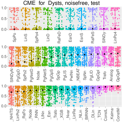
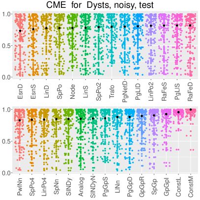
Figure 2: The $\mathsf{CME}$-values for each tuned method applied to the test data of the Dysts database of 133 chaotic systems in the noisefree and noisy versions. Methods with hyperparameters were tuned on the respective tune dataset of each system. The methods are ordered by the median $\mathsf{CME}$ over the 133 systems, shown in black.

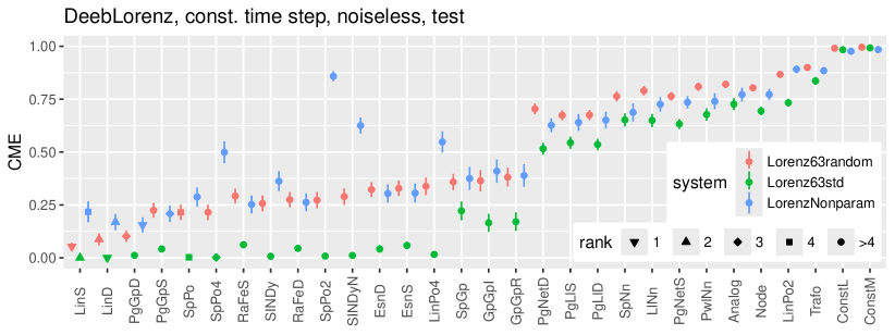
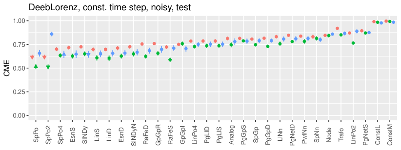
Figure 3: Mean $\mathsf{CME}$ of 100 repetitions with $95\%$ confidence intervals for the constant timestep data from DeebLorenz. Each method is applied the test data of each of the three systems of the database in the noisefree and noisy versions after tuning was executed on the respective tune data. The results are ordered by the median of the error over the three systems.

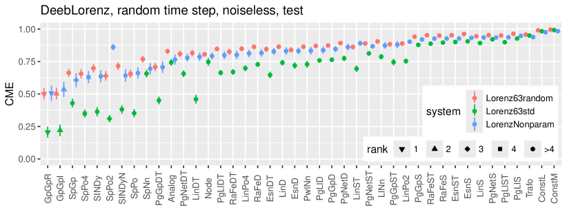
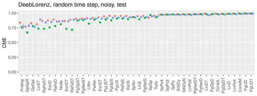
Figure 4: Same as Figure 3 but with the observation schemes which use random timesteps.

3.1 Lightweight Methods Outperform Heavyweight Methods

In all settings with constant timestep, the best methods are rather simple (e.g., SpPo, LinS, EsnS, …) and have low computational costs. In contrast, more complex, high-end learning methods (Node, Trafo, PgNet, _NBEAT, _NHiTS, _RaFo, _Node, _RNN, _Trafo, _XGB, _BIRNN, _TCN) perform rather poorly. This questions the utility of the latter group of methods for low dimensional systems, in particular, when considering the high computational demand.

3.2 Comparison to [Gil23]

Compared to the results of [Gil23] (the method names starting with underscore in Figure 2), several methods examined here have much lower errors: For the noisefree Dysts data, the median $\mathsf{CME}$ of _NBEAT, the best performing method in [Gil23], is 0.587. The lowest error achieved in our simulations is 0.004 (SpPo). A reason for this is the higher effort in our hyperparameter tuning compared to the one in [Gil23], where only one parameter per method was optimized. We allow for more hyperparameter optimization, in particular for methods with low computational costs. But note that SpPo4 and LinPo4 are tuning-free methods and achieve median $\mathsf{CME}$s of 0.008 and 0.039, respectively. Furthermore, from all methods of [Gil23], only _NBEAT outperforms the baseline method Analog. This underlines the importance of the choice of appropriate methods and baselines for a given task.

3.3 Importance of Hyperparameter Optimization for some Methods

Let us compare the median $\mathsf{CME}$ for selected methods on the noisefree dataset of Dysts, see Figure 2, Table 20, and Table 22. The methods _Nvar (0.83) and _Esn (0.80) from [Gil23] are essentially the same as our LinS (0.0054) and EsnS (0.026), respectively. But for the latter more hyperparameters were tuned. Our simulation shows a median $\mathsf{CME}$ orders magnitude lower than for the respective methods in [Gil23]. From this we conclude that tuning relevant hyperparameters is crucial for these methods.

3.4 Tuning-free Methods

Apart from the baselines, following methods are tuning-free: SpPo2, SpPo4, PwNn, SpNn, LinPo2, LinPo4. In all noise-free settings, SpPo4 is among the best. SpPo2 performs well in parametric noisy settings with constant timestep. The methods PwNn and SpNn are mediocre, usually having lower $\mathsf{CME}$ than the baselines and the worst methods, but never close to the best. LinPo2 often performs poorly whereas LinPo4 is mostly in the better half of methods.

As these methods come with lower computational costs, are simple to implement, and show good performance, we recommend SpPo2, SpPo4, and LinPo4 to be used as additional baselines for task similar to those shown in this study.

3.5 Polynomials

Most systems in Dysts and all systems but LorenzNonparam in DeebLorenz have model function $f$ that is a polynomial of low degree. Thus, it is not surprising that methods based on this assumption such as SpPo and SINDy perform well on these tasks. Note that a polynomial model function $f$ does not imply that the propagator $\mathcal{P}_{\Delta\!t}$ for a given timestep $\Delta\!t$ is also polynomial. Still, it might be a reasonable approximation, which would also explain the good performance of Lin*. Focusing on LorenzNonparam, SpPo and SINDy seem to have a somewhat weaker performance than on the parametric systems. The fit of a polynomial with degree 2 in SpPo2, which is enough for Lorenz63std and Lorenz63random has the clearest reduction in performance when it is applied to LorenzNonparam.

Thus, low degree polynomial approximation works only well if the target function can truly be described as such a polynomial. For higher degree polynomial approximation the effect is much less pronounced (note Taylor’s approximation theorem), but inherently nonparametric methods such as GpGp* or PgGp* may be more suitable if the target is non-polynomial.

3.6 Noise vs No Noise

In the absence of noise, forecasting becomes an interpolation task, whereas noisy observations yield a regression problem. Generally, performance degrades strongly when noise is added to the observations. Moreover, methods that are best for the noisefree interpolation task are typically not the best for the noisy regression task.

The Esn* has access to states of the past, whereas the otherwise similar method RaFe* does not. Because of the Markovian nature of our dynamical systems, knowledge of the past is not required in the noisefree case as the next state is equal to the (true) propagator applied to the current state. This is reflected in our simulation results, where RaFe* tends to perform better than Esn* in noisefree settings and vice versa for the settings with measurement noise. As the noisy systems of Dysts are created with system noise, they are Markovian. Surprisingly, the Esn* seems to be at an advantage over RaFe* here, too.

Under noise, the lower degree polynomial SpPo2 performs relatively better than the higher degree polynomial SpPo4, and vice versa in the noisefree case. Overfitting, which can only happen in the noisy case, seems to be the reason for this observation.

3.7 Fixed vs Random Timestep

There is a noticeable difference in performances of methods between fixed and random timesteps. Generally, random timesteps make the forecasting task more difficult. But also the rank of methods according to their $\mathsf{CME}$ changes: The Gaussian process based methods GpGp* take the lead for random timesteps. For fixed timesteps, these methods are only mediocre.

As could be expected, propagator methods that do not have the timestep as an input, do not fare well if the timestep is not constant. With the additional knowledge of the timestep (*ST and *DT), the performance improves, but not to the level of the best solution smoothers.

The combination of a random timestep with noisy observations seems to make the learning task so difficult that only very few methods are able to beat the baseline Analog. In the case of Lorenz63random, only GpGpR, GpGpI, and LinST have better scores. For LorenzNonparam only one method, GpGpI, is able to improve upon the result of Analog.

3.8 Different Modes for Propagators

As could be expected, the errors of propagators with and without timestep input (Table 26) are similar when the timestep is constant. For random timesteps, knowledge of the timestep typically improves the results.

Between the state (*S*) and the difference quotient (*D*) versions of the propagator estimators (Table 28), there is no clear overall winner and the results of the two methods are fairly close. But in the case of random timesteps without noise, *D* always has the lower errors. The reason for this seems to be, that the estimation of the difference quotient reduces the depends of the target on the timestep.

3.9 SINDy and Sparsity

According to Table 31, simple solutions smoothers mostly outperform those with thresholding (SINDy, SINDyN). Curiously, in the nonparametric setting LorenzNonparam, SINDy has one of the better rankings among the polynomial solutions smoothers. But the differences in mean $\mathsf{CME}$ are not statistically significant.

SINDyN (with normalization) is usually worse than SINDy. This makes sense, as many systems studied here have sparse polynomial dynamics and normalization (which in our case includes rotation) destroys sparsity.

3.10 Different Error Measures

When ranking different methods according to their performance, the error metrics $\mathsf{CME}$, $\mathsf{sMAPE}$, and $t_{\mathsf{valid}}$ yield similar results. A noticeable difference can be observed between $\mathsf{sMAPE}$ and the other two for difficult tasks because $\mathsf{sMAPE}$ punishes divergence more severely, see Table 18. From the explicit error values in Table 20, we see that $t_{\mathsf{valid}}$ is less suitable for distinction of well-performing methods if the testing time is not long enough and the threshold parameter too lenient, as several methods achieve the maximal valid time.

3.11 Computational Demand

If computational resources are a concern, the high-end machine learning methods Trafo and Node may not be suitable choices for estimators (even when hyperparameter tuning is ignored), see Table 34 and Table 36. Furthermore, their performance on the problems in this study is generally mediocre at best. Note that we are considering low dimensional problems here ($d=3$ for DeebLorenz, and $3\leq d\leq 10$ for Dysts). Most of the lightweight algorithms solve a system of linear equations $Ax=b$ with $A\in\mathbb{R}^{p\times p}$. Here $p$ is the number of features, which typically grows at least linearly in $d$. The computational complexity of solving the linear equation is typically cubic in $p$ (but at least quadratic). This means, without further adjustment of the algorithms (e.g., only approximating the solution), most algorithms tested here require unfeasible computational resources in high dimensions. But neural network based algorithms are known to scale well with dimension, suggesting a potential use case for Trafo and Node.

3.12 Tuning vs Evaluation

Unsurprisingly, the error measures of tuned methods are better on the tuning dataset than on the evaluation datasets, see Table 20. For some methods, the difference is rather large (for EsnS, we have a median $\mathsf{CME}$ of $0.0046$ on the noisefree Dysts tune data and $0.026$ on the evaluation data). In combination with the high number of parameters tested for these methods (for EsnS on the noisefree Dysts data, $288.5$ per system on average), this suggests that the hyperparameter tuning has the potential to introduce overfitting on the tuning data. This affects Dysts more than DeebLorenz as there is much less tuning data for the former.

3.13 Lorenz63std vs Lorenz63random

Even though Lorenz63std and Lorenz63random have the same functional form of their model function $f$, only differing in polynomial coefficients, absolute errors and relative rankings of methods differ strongly between the two systems (Figure 3, Figure 4).

Tuning for Lorenz63random (and LorenzNonparam) is difficult in that the tuned parameters must work well for similar but different (randomly chosen) systems. The dynamics in Lorenz63std are fixed so that essentially not only the functional form of $f$ but also the specific coefficients of the polynomial could be (partially) inferred during tuning.

In conclusion, a low $\mathsf{CME}$ value for Lorenz63random is a more robust indicator of good performance than a low $\mathsf{CME}$ value for Lorenz63std.

3.14 Uncertainty

As there is only on repetition available in the Dysts database, reported differences between the performance of methods might not be robust on the same system. Furthermore, confidence intervals based on the results on the 133 systems are hard to justify as one typically assumes a independent, identical distribution of the considered values. But note that the code for generating more data for Dysts is available at the respective repository.

In contrast, for DeebLorenz, experiments for the same system and observation scheme are repeated 100 times with randomly drawn initial conditions, noise values, and timesteps (if applicable). This allows us to judge, whether reported differences in $\mathsf{CME}$ values are statistically significant. In Figure 6, we visualize the results of paired $t$-Tests for the null hypothesis $\mathsf{CME}(\text{{Method1}})\geq\mathsf{CME}(\text{{Method2}})$. If the null can be rejected, it shows that Method1 is significantly better Method2 on the given system with the given observation scheme using the $\mathsf{CME}$ as error metric. We see that the ranking of the algorithms as shown in Table 12 is mostly robust up to permutation of two or three consecutive ranks. In comparison, Figure 7 shows that only 10 repetitions would yield largely indistinguishable performances.

As an example, ranks 1 to 6 for the noisefree observation scheme with constant timestep for the system Lorenz63random (100 repetitions) are LinST, LinS, LinD, LinDT, PgGpDT, and PgGpD. From top left 6 by 6 pixel matrix of the first image in the second row of Figure 6, we can conclude the following: The methods LinST, LinS are not statistically distinguishable and neither are LinD, LinDT, PgGpDT, PgGpD. But LinS is significantly better than PgGpD.

All in all, it seems prudent to repeat experiments to obtain more reliable results and be able to judge the confidence of these results.

Appendix A The Datasets

A.1 Dysts

The Dysts datasets consist of 133 chaotic systems with state space dimension between $3$ and $10$. See Table 1. For a detailed description of the Dysts dataset, see [Gil21]. Here we comment on some peculiarities of the database, in particular the noisy version.

dimension	3	4	5	6	10
# systems	102	19	2	3	7

Table 1: Number of systems in Dysts with a given dimension.

1. In the noisy version of the data, the system MacArthur is divergent (oscillating state values in the order of magnitude $\pm 10^{100}$ and higher). Moreover, for CircadianRhythm and DoublePendulum, the variance of the solutions increases by multiple orders of magnitude between the noisefree and noisy version.

2. For the noisefree dataset, the most difficult to learn systems seem to be MacArthur, LidDrivenCavityFlow, and IkedaDelay, which all have values $0.9<\mathsf{CME}<0.99$ for the best methods in this study.

3. For following systems from the noisy dataset, learning seems impossible (best method with $\mathsf{CME}>0.99$): DoublePendulum, ArnoldBeltramiChildress, BickleyJet, ArnoldWeb, YuWang. Curiously, the oscillating behavior of MacArthur makes this system rather predictable with a best $\mathsf{CME}$ of $0.13$ achieved by EsnS.

A.2 DeebLorenz

The dataset consists of three systems and four observation schemes and is separated into tuning and testing data with 10 and 100 replications, respectively.

Each system is described by an autonomous, first-order, three-dimensional ODE of the form

$$\dot{u}(t)=f(u(t))\,,\quad\text{for }t\in\mathbb{R}\,,$$

where $f\colon\mathbb{R}^{3}\to\mathbb{R}^{3}$ is the model function and the solution $u\colon\mathbb{R}\to\mathbb{R}^{3}$ describes the state of the system over time. For the three systems, the model functions $f$ are created as follows:

• Lorenz63std: The Lorenz63 system in its standard definition [Lor63], i.e.,

  $$f(u)=\begin{pmatrix}\sigma(u_{2}-u_{1})\\ u_{1}(\rho-u_{3})-u_{2}\\ u_{1}u_{2}-\beta u_{3}\end{pmatrix}$$ (12)

  with $\sigma=10$, $\rho=28$, $\beta=8/3$.

• Lorenz63random: As Lorenz63std, but for each replication, the three parameters are drawn uniformly at random from an interval,

  $$\sigma\sim\mathsf{Unif}([5,15])\,,\quad\rho\sim\mathsf{Unif}([20,80])\,,\quad\beta\sim\mathsf{Unif}([2,6])\,.$$ (13)

  These intervals are chosen so that the resulting systems exhibit chaotic behavior.

• LorenzNonparam: As Lorenz63std, but the parameters depend on the state, $\sigma=\sigma(u)$, $\rho=\rho(u)$, $\beta=\beta(u)$. For each replication, the functions $\sigma,\rho,\beta\colon\mathbb{R}^{3}\to\mathbb{R}$ are sampled from a Gaussian process so that the (non-constant) parameter values are in (or at least close to) the intervals sampled from in (13). To make sure, that the sampled model functions lead to interesting systems, we reject results where the trajectory of given initial states seem to approach a fixed point. The resulting trajectories all seem to exhibit chaotic behavior.

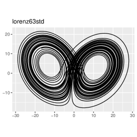
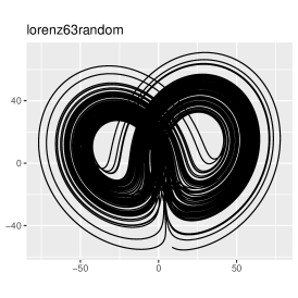
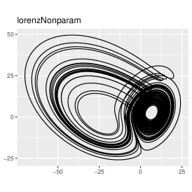
Figure 5: Trajectories $u(t)$ of the three models of DeebLorenz with $t\in[0,50]$. The 3-dimensional state space is projected to the 2-dimensional subspace with highest variance.

Note that the model functions of Lorenz63std and Lorenz63random are polynomials of degree two with 23 out of 30 coefficients equal to zero, whereas instances of the model function of LorenzNonparam cannot be described by a polynomial of finite degree.

To obtain one replication of one of the systems, $f$ is set or sampled as described above. Then initial conditions $u_{0}$ are sampled uniformly at random from the Lorenz63 attractor (as a proxy for the attractors of the other variations of the Lorenz63 system). The initial value problem $\dot{u}=f(u)$, $u(0)=u_{0}$ is solved using a fourth order Runge-Kutta numerical ODE solver with timestep $10^{-3}$. If timesteps are random, they are sampled from an exponential distribution $\Delta\!t_{i}\sim\mathsf{Exp}(\lambda)$ with rate parameter $\lambda=\Delta\!t_{0}^{-1}$ and $\Delta\!t_{0}=0.01$. If the stepsize is constant, we set $\Delta\!t_{i}=\Delta\!t_{0}$. We set $t_{0}=0$ and $t_{i}=t_{i-1}+\Delta\!t_{i}$. The last observation $t_{n}$ is chosen such that $t_{n+1}\geq T$ where $T=100$. The number of observations is $n=10^{4}$ (exactly, for constant timesteps, and, in expectation, for random time steps). For noisy observations, we draw independent noise from a multivariate normal distribution, $\epsilon_{i}\sim\mathcal{N}(0,\sigma^{2}I_{3})$ with standard deviation $\sigma=0.1$, where $I_{3}$ is the $3\times 3$ identity matrix. For the noisefree observation scheme, we set $\epsilon_{i}=0$. Then the observations are $Y_{i}=u(t_{i})+\epsilon_{i}$. For testing, we also record $u(t_{j})$, where $t_{j}=T+(j-n)\Delta\!t_{0}$, $j=n+1,\dots,n+m$, and $m=10^{3}$.

Appendix B Methods

B.1 Implementation

All methods are implemented in R [R ̵C24], except for Node, which is implemented in Julia [Bez+17]. Furthermore, PgNet*, Trafo use Keras [Cho+15] (via its R-interface). All code is available in the public git repositories on GitHub as listed in Table 2.

chroetz/DEEBdata	generation of DeebLorenz
chroetz/DEEBcmd	command line interface for the other packages
chroetz/DEEBesti	estimation methods
chroetz/DEEBeval	evaluate predictions
chroetz/DEEBtrajs	handling the csv-files containing observations and predictions
chroetz/DEEB.jl	the Julia implementation of the neural ODE
chroetz/ConfigOpts	handling the json-files containing settings for methods

Table 2: GitHub repositories containing the code used in this study.

B.2 Normalization

For all methods except SINDy, we calculate an affine linear normalization from the training data: Let $\hat{\mu}=\frac{1}{n}\sum_{i=1}^{n}Y_{i}$ be the empirical mean and $\hat{\Sigma}=\frac{1}{n-1}\sum_{i=1}^{n}(Y_{i}-\hat{\mu})(Y_{i}-\hat{\mu})^{\!\top}\!$ the empirical covariance matrix. Then the normalized data is

$$\bar{Y}_{i}:=\hat{\Sigma}^{-\frac{1}{2}}\left(Y_{i}-\hat{\mu}\right)\,.$$ (14)

It has mean zero and an identity covariance matrix. A prediction $\bar{u}(t_{j})$ from a given method trained on the normalized data is transformed back by

$$\hat{u}(t_{j}):=\hat{\Sigma}^{\frac{1}{2}}\bar{u}(t_{j})+\hat{\mu}\,.$$ (15)

To not destroy potential sparsity, we only scale the inputs to SINDy by the inverse of the square root of $\hat{\sigma}^{2}=\frac{1}{n-1}\sum_{i=1}^{n}Y_{i}^{\!\top}\!Y_{i}$.

B.3 Propagator

For propagator based methods, a mapping from the current state to the next one is learned. The target is either directly the next state (suffix S) or the increment scaled by the inverse of the time step (suffix D). Additionally to the current (and potentially past) state(s), the time step can also serves as a predictor (suffix T). See also Section 2.3.

B.4 Analog

• Alternative names: Analogue, analog method

• Parameters: margin $\omega\in\mathbb{N}$

• tuning: categorical, persistent: $\omega\in\{1,10,100\}$.

• Description: Initialize $x\leftarrow u(T)$ and $j_{0}\leftarrow 0$. Let $k=\operatorname*{arg\,min}_{i\in{\left\llbracket n-\omega\right\rrbracket}}\|Y_{i}-x\|_{2}$. Set $\hat{u}(t_{j_{0}+j})=Y_{k+j}$ for $j\in{\left\llbracket j_{\mathsf{max}}\right\rrbracket}$, $j_{\mathsf{max}}:=\min(n-k,m)$. If the prediction time series is not yet complete, repeat with $x\leftarrow Y_{k+j_{\mathsf{max}}}$ and $j_{0}\leftarrow j_{0}+j_{\mathsf{max}}$.

B.5 Node

• Alternative names: Neural ODE

• Parameters:

  • number of hidden layers: $L$

  • width of hidden layers: $W$

  • activation function: swish

  • weight decay $10^{-6}$

  • ODE solver steps for the loss: $S$

  • epochs: $400$

  • Optimizer: AdamW

  • learning rate: $10^{-}3$

  • internal training–validation to use weights with lowest validation error: 85% – 15%

• Tuning:

  • categorical, yielding: $(L,W)\in\{(2,32),(4,32),(2,128)\}$

  • scalar, exponential (factor $2$): $S=1,2$, $S\in[1,64]$

• Description: See [Che+18]. We use a Julia implementation.

B.6 PgGp*

• Alternative names: GpPropa_state, GpPropa_state_time, GpPropa_deriv, GpPropa_deriv_time

• Parameters:

  • bandwidth: $h$

  • kernel function: $x\mapsto\exp(x^{2}/(2h^{2}))$

  • regularization: $\lambda$

• Tuning:

  • scalar, exponential (factor $2$): $h=0.05,0.2,0.8$, $10^{-4}\leq h\leq 10$

  • scalar, exponential (factor $10$): $\lambda=10^{-12},10^{-8},10^{-4}$, $10^{-15}\leq\lambda\leq 10^{2}$

• Description: A propagator estimator (section B.3) using a Gaussian process [RW05].

B.7 PgNet*

• Alternative names: NeuralNetPropa_state, NeuralNetPropa_state_time, NeuralNetPropa_deriv, NeuralNetPropa_deriv_time

• Parameters:

  • batch size: 32

  • epochs: 1000,

  • training – validation split: 90% – 10%

  • architecture (tuple of layer width): $w$

  • activation function: swish

  • learning rate $2\cdot 10^{-4}$

• Tuning: categorical, yielding: $w=(32,64,64,32),(128,128),(64,128,64)$

• Description: A propagator estimator (section B.3) using a vanilla feed-forward neural network implemented using Keras.

B.8 PgLl*

• Alternative names: LocalLinearPropa_state, LocalLinearPropa_state_time, LocalLinearPropa_deriv, LocalLinearPropa_deriv_time

• Parameters:

  • kernel function: $x\mapsto\exp(x^{2}/h^{2})$

  • bandwidth: $h$

  • neighbors: $k=50$

• Tuning:

  • scalar, exponential (factor $2$): $h=0.05,0.2,0.8$, $h\in[10^{-4},10]$

• Description: A propagator estimator (section B.3) using a local linear estimator. Locality is introduced by the kernel weights and a $k$-nearest neighbors restriction. The latter is used to keep the computational demand low.

B.9 Lin*

• Alternative names: Linear_state, Linear_state_time, Linear_deriv, Linear_deriv_time

• Parameters:

  • past steps $K$

  • skip steps $s$

  • polynomial degree $\ell$

  • penalty $\lambda$

• Tuning:

  • scalar, linear (step $1$): $K=0,1,4$, $0\leq K\leq 32$

  • scalar, linear (step $1$): $s=1,2$, $1\leq s\leq 9$

  • scalar, linear (step $1$): $\ell=1,4$, $1\leq\ell\leq 8$

  • scalar, exponential (factor $10$): $\lambda=10^{-12},10^{-8},10^{-4}$, $10^{-15}\leq\lambda\leq 10^{2}$

• Description: A propagator estimator (section B.3) using Ridge regression (linear regression with $L_{2}$-penalty with weight $\lambda$) on polynomial features of degree at most $\ell$ of the current at time $t_{i}$ and past states $t_{i-sk}$, $k\in{\left\llbracket K\right\rrbracket}$.

B.10 LinPo2, LinPo4

• Alternative names: Linear_Poly2, Linear_Poly4

• Parameters: as in section B.9 with $K=0$, $s=1$, $\ell=2$ and $\ell=4$, $\lambda=0$

• Tuning: none

• Description: As Lin* (section B.9), but with fixed hyperparameters.

B.11 RaFe*

• Alternative names: RandomFeatures_state, RandomFeatures_state_time, RandomFeatures_deriv, RandomFeatures_deriv_time

• Parameters:

  • number of neurons: 400

  • input weight scale $c$

  • penalty $\lambda$

  • forward skip $s$

  • random seed $r$

• Tuning:

  • scalar, exponential (factor $2$): $c=0.025,0.1,0.4$, $10^{-7}\leq c\leq 10^{2}$

  • scalar, exponential (factor $10$): $\lambda=10^{-12},10^{-8},10^{-4}$, $10^{-15}\leq\lambda\leq 10^{2}$

  • scalar, exponential (factor $2$): $s=0,1$, $1\leq s\leq 64$

  • categorical, persistent: $r=1,2,3,4$

• Description: A propagator estimator (section B.3) using random feature regression, i.e., Ridge regression on features created from an untrained vanilla feed forward neural network with 1 layer of $\ell$ neurons.

B.12 Esn*

• Alternative names: Echo state network, reservoir computer, Esn_state, Esn_state_time, Esn_deriv, Esn_deriv_time

• Parameters:

  • number of neurons: $400$

  • node degree: $6$

  • spectral radius: $0.1$

  • input weight scale $c$

  • penalty $\lambda$

  • forward skip $s$

  • random seed $r$

• Tuning: same as RaFe* (section B.11)

• Description: See [Jae01].

B.13 Trafo

• Alternative names: Transformer

• Parameters:

  • context length: $\ell$,

  • position dimension: $d_{\mathsf{pos}}$

  • head size: $s_{\mathsf{head}}$

  • number of heads: $n_{\mathsf{head}}$

  • number of blocks: $n_{\mathsf{block}}=4$

  • number of neurons in the MLP-layers: $n_{\mathsf{mlp}}$

  • dropout parameter: $0.1$

  • learning rate: $\lambda$

  • training–validation split: 90% – 10%

  • epochs: $400$

  • batch size: $32$

  • positional encoding: sinusoidal

  • loss: MSE

  • optimizer: Adam

• Tuning: We test the hyperparameter combinations $(\ell,d_{\mathsf{pos}},s_{\mathsf{head}},n_{\mathsf{head}},n_{\mathsf{mlp}},\lambda)$ given in the rows of Table 3.

• Description: We use a Keras-implementation of a transformer network. As an input, we take the states at times $t_{k-\ell+1},\dots,t_{k}$ and add a sinusoidal positional encoding of dimension $d_{\mathsf{pos}}$ by appending it to each of the state vectors. The network consist of $n_{\mathsf{block}}$-many consecutive blocks consisting of an attention layer (followed by layer normalization) and a dense MLP-layer with ReLu activation (followed by layer normalization). The attention layers have $n_{\mathsf{head}}$-many heads of size $s_{\mathsf{head}}$.

$\ell$	$d_{\mathsf{pos}}$	$s_{\mathsf{head}}$	$n_{\mathsf{head}}$	$n_{\mathsf{mlp}}$	$\lambda$
$64$	$16$	$64$	$4$	$32$	$10^{-3}$
$32$	$8$	$32$	$16$	$32$	$10^{-4}$
$32$	$32$	$16$	$16$	$32$	$10^{-4}$
$32$	$8$	$16$	$16$	$32$	$10^{-3}$
$32$	$8$	$32$	$8$	$64$	$10^{-4}$

Table 3: Hyperparameters for the Transformer Trafo.

B.14 PwNn

• Alternative names: PwLin-Nn

• Parameters: none.

• Tuning: none.

• Description: A solution smoother using piece-wise linear interpolation for estimating the solution $u$ and a nearest neighbor interpolation for estimating the model function $f$.

B.15 SpNn

• Alternative names: Spline-Nn

• Parameters: none.

• Tuning: none.

• Description: A solution smoother using a cubic spline interpolation for estimating the solution $u$ and a nearest neighbor interpolation for estimating the model function $f$.

B.16 LlNn

• Alternative names: Ll-Nn

• Parameters:

  • kernel function: $x\mapsto\exp(x^{2}/h^{2})$

  • bandwidth: $h$

• Tuning:

  • scalar, exponential (factor $2$): $h=0.05,0.2,0.8$, $10^{-4}\leq h\leq 10$

• Description: A solution smoother using local linear regression for estimating the solution $u$ and a nearest neighbor interpolation for estimating the model function $f$.

B.17 SpPo

• Alternative names: Spline-Poly

• Parameters:

  • polynomial degree $\ell$

  • penalty $\lambda$

• Tuning:

  • scalar, linear (step $1$): $\ell=2,3,4$, $1\leq\ell\leq 8$

  • scalar, exponential (factor $10$): $\lambda=10^{-12},10^{-8},10^{-4}$, $10^{-15}\leq\lambda\leq 10^{2}$

• Description: A solution smoother using a cubic spline interpolation for estimating the solution $u$ and Ridge regression with polynomial features for estimating the model function $f$.

B.18 SpPo2, SpPo4

• Alternative names: Spline-Poly2 / Spline-Poly4

• Parameters: as in section B.17 with $\ell=2$ and $\ell=4$, $\lambda=0$

• Tuning: none

• Description: As SpPo* (section B.17), but with fixed hyperparameters.

B.19 SpGp

• Alternative names: Spline-Gp

• Parameters:

  • bandwidth: $h$

  • neighbors:$k=50$

  • kernel function: $x\mapsto\exp(x^{2}/(2h^{2}))$

  • regularization: $\lambda$

• Tuning:

  • scalar, exponential (factor $2$): $h=0.05,0.2,0.8$, $10^{-4}\leq h\leq 10$

  • scalar, exponential (factor $10$): $\lambda=10^{-12},10^{-8},10^{-4}$, $10^{-15}\leq\lambda\leq 10^{2}$

• Description: A solution smoother using a cubic spline interpolation for estimating the solution $u$ and Gaussian process regression for estimating the model function $f$. To make the Gaussian process computationally efficient, we localize it by only considering the $k$ nearest neighbors for an evaluation.

B.20 GpGpI, GpGpR

• Alternative names: Gp-Gp-interp / Gp-Gp-regress

• Parameters:

  • bandwidth: $h$

  • neighbors:$k=50$

  • kernel function: $x\mapsto\exp(x^{2}/(2h^{2}))$

  • regularization: $\lambda$

  • solution bandwidth: $0.1$

  • solution regularization $\mu$

• Tuning:

  • scalar, exponential (factor $2$): $h=0.05,0.2,0.8$, $10^{-4}\leq h\leq 10$

  • scalar, exponential (factor $10$):

    • for GpGpI: $\lambda=10^{-14},10^{-13},10^{-12}$, $10^{-15}\leq\lambda\leq 10^{-8}$

    • for GpGpR: $\lambda=10^{-12},10^{-8},10^{-4}$, $10^{-15}\leq\lambda\leq 10^{2}$

  • scalar, exponential (factor $10$):

    • for GpGpI: $\mu=10^{-14},10^{-13},10^{-12}$, $10^{-15}\leq\mu\leq 10^{-8}$

    • for GpGpR: $\mu=10^{-12},10^{-8},10^{-4}$, $10^{-15}\leq\mu\leq 10^{2}$

• Description: A solution smoother using Gaussian process regression for estimating the solution $u$ and Gaussian process regression for estimating the model function $f$. To make the second Gaussian process computationally efficient, we localize it by only considering the $k$ nearest neighbors for an evaluation.

B.21 SINDy, SINDyN

• Alternative names: Spline-ThreshLm / Spline-ThreshLmRotate

• Parameters:

  • polynomial degree: $5$

  • thresholding iterations: $100$

  • threshold $\tau$

• Tuning:

  • scalar, exponential (factor $2$): $\tau=0.04,0.16,0.64$, $10^{-7}\leq\tau\leq 10^{2}$

• Description: A solution smoother using a cubic spline interpolation for estimating the solution $u$ and sparse linear regression with polynomial features for estimating the model function $f$. See [BPK16].

Appendix C Further Details of the Results

In this section we list additional tables and plots the show the results of the simulation study in more detail. In the tables we will make use of the short notation given in Table 4.

short	database	system	noise	timestep
DF	Dysts	all	noisefree	constant
DY	Dysts	all	noisy	constant
LS1	DeebLorenz	Lorenz63std	noisefree	constant
LS2	DeebLorenz	Lorenz63std	noisy	constant
LS3	DeebLorenz	Lorenz63std	noisefree	random
LS4	DeebLorenz	Lorenz63std	noisy	random
LR1	DeebLorenz	Lorenz63random	noisefree	constant
LR2	DeebLorenz	Lorenz63random	noisy	constant
LR3	DeebLorenz	Lorenz63random	noisefree	random
LR4	DeebLorenz	Lorenz63random	noisy	random
LN1	DeebLorenz	LorenzNonparam	noisefree	constant
LN2	DeebLorenz	LorenzNonparam	noisy	constant
LN3	DeebLorenz	LorenzNonparam	noisefree	random
LN4	DeebLorenz	LorenzNonparam	noisy	random

Table 4: Short notation for databases, systems, and observation schemes in the tables of Appendix C.

Mean error values ($\mathsf{CME}$, $\mathsf{sMAPE}$, $t_{\mathsf{valid}}$) for DeebLorenz are shown in Table 6, Table 8, Table 10. The respective rankings are displayed in Table 12, Table 14, Table 16. Furthermore, Table 18 shows the ranks for all error metric side by side and highlights the strongest disagreement.

For Dysts, the median error values over all systems are shown in Table 20, Table 22, and Table 24. These tables also include the value of the error metrics on the tuning data.

Table 26 and Table 28 detail the performances of the different modes of propagator based methods. And Table 31 focuses on polynomial solution smoothers.

Results of statistical tests for distinguishing the performances of methods on DeebLorenz are shown in Figure 6 and Figure 7.

Computational cost for tuning is listed in Table 34.

Table 5: *

CME Values
Method	median	LS1	LR1	LN1	LS2	LR2	LN2	LS3	LR3	LN3	LS4	LR4	LN4
GpGpR	0.58	0.17	0.38	0.39	0.66	0.76	0.70	0.21	0.50	0.51	0.67	0.77	0.79
GpGpI	0.62	0.17	0.36	0.41	0.76	0.75	0.71	0.22	0.50	0.53	0.78	0.83	0.77
SpPo	0.64	0.0026	0.22	0.29	0.51	0.62	0.66	0.35	0.65	0.66	0.98	0.98	0.97
SpPo4	0.64	0.0019	0.22	0.50	0.63	0.70	0.64	0.35	0.66	0.63	0.98	0.98	0.97
SINDy	0.65	0.0072	0.26	0.36	0.65	0.72	0.64	0.36	0.70	0.64	0.98	0.98	0.97
LinDT	0.65	0.000062	0.10	0.17	0.58	0.70	0.60	0.46	0.82	0.79	0.98	0.99	0.97
SINDyN	0.66	0.011	0.29	0.63	0.65	0.73	0.67	0.38	0.72	0.64	0.98	0.98	0.97
EsnDT	0.68	0.038	0.34	0.32	0.61	0.71	0.64	0.65	0.85	0.83	0.74	0.87	0.86
LinST	0.70	0.00015	0.053	0.22	0.58	0.70	0.62	0.69	0.86	0.89	0.74	0.81	0.89
SpGp	0.71	0.22	0.36	0.38	0.75	0.81	0.79	0.43	0.66	0.61	0.97	0.92	0.95
RaFeDT	0.71	0.045	0.28	0.27	0.63	0.75	0.68	0.67	0.82	0.80	0.73	0.87	0.84
EsnD	0.72	0.042	0.32	0.30	0.63	0.71	0.66	0.72	0.84	0.83	0.76	0.88	0.85
LinD	0.72	0.000035	0.087	0.17	0.60	0.70	0.66	0.74	0.86	0.83	0.99	0.98	0.98
PgGpDT	0.72	0.012	0.10	0.16	0.74	0.78	0.79	0.45	0.71	0.71	0.98	0.99	0.98
RaFeST	0.74	0.062	0.26	0.26	0.63	0.75	0.71	0.89	0.95	0.93	0.72	0.89	0.89
RaFeD	0.74	0.045	0.27	0.26	0.62	0.75	0.68	0.73	0.86	0.82	0.78	0.89	0.86
SpPo2	0.75	0.0081	0.27	0.86	0.51	0.62	0.86	0.31	0.64	0.86	0.98	0.98	0.97
LinPo4	0.77	0.016	0.34	0.55	0.73	0.78	0.75	0.70	0.85	0.81	0.99	0.99	0.98
PgLlDT	0.77	0.59	0.67	0.68	0.74	0.79	0.75	0.66	0.85	0.80	0.99	0.99	0.99
Analog	0.77	0.73	0.82	0.77	0.75	0.81	0.78	0.74	0.83	0.77	0.76	0.84	0.77
PgLlD	0.77	0.54	0.67	0.65	0.74	0.79	0.75	0.76	0.87	0.84	0.99	0.99	0.99
SpNn	0.78	0.65	0.76	0.69	0.81	0.83	0.80	0.66	0.77	0.69	0.93	0.93	0.93
EsnST	0.79	0.11	0.29	0.32	0.59	0.73	0.64	0.90	0.95	0.93	0.84	0.93	0.91
LinS	0.79	0.00015	0.053	0.22	0.61	0.70	0.65	0.89	0.95	0.93	0.90	0.95	0.93
PgGpST	0.80	0.042	0.22	0.21	0.79	0.81	0.78	0.75	0.88	0.88	0.87	0.90	0.89
PgGpD	0.80	0.012	0.10	0.16	0.73	0.82	0.79	0.76	0.87	0.85	0.98	0.97	0.99
PgNetDT	0.80	0.54	0.68	0.61	0.80	0.85	0.83	0.66	0.81	0.78	0.98	0.98	0.98
EsnS	0.81	0.058	0.33	0.31	0.63	0.72	0.65	0.91	0.96	0.93	0.90	0.95	0.93
Node	0.81	0.69	0.80	0.77	0.84	0.85	0.86	0.68	0.81	0.79	0.81	0.86	0.85
RaFeS	0.81	0.062	0.29	0.25	0.59	0.72	0.71	0.90	0.95	0.93	0.91	0.95	0.93
LlNn	0.81	0.65	0.79	0.73	0.76	0.83	0.81	0.79	0.90	0.87	0.82	0.91	0.90
PwlNn	0.82	0.68	0.81	0.74	0.78	0.84	0.81	0.73	0.86	0.83	0.89	0.92	0.91
PgNetD	0.83	0.52	0.70	0.63	0.78	0.85	0.81	0.77	0.89	0.86	0.98	0.98	0.98
PgLlST	0.84	0.48	0.65	0.60	0.74	0.78	0.75	0.90	0.95	0.94	0.89	0.95	0.92
PgGpS	0.85	0.042	0.22	0.21	0.79	0.81	0.78	0.88	0.94	0.92	0.88	0.95	0.92
PgLlS	0.85	0.54	0.67	0.64	0.74	0.79	0.75	0.93	0.96	0.95	0.91	0.95	0.92
PgNetST	0.87	0.65	0.76	0.75	0.87	0.89	0.87	0.81	0.89	0.87	0.88	0.91	0.90
LinPo2	0.89	0.73	0.87	0.89	0.76	0.87	0.89	0.75	0.89	0.90	0.98	0.98	0.97
PgNetS	0.91	0.63	0.76	0.74	0.87	0.89	0.87	0.92	0.95	0.94	0.92	0.95	0.93
Trafo	0.93	0.84	0.90	0.88	0.85	0.92	0.87	0.95	0.96	0.94	0.93	0.96	0.95
ConstL	0.98	0.98	0.99	0.98	0.98	0.99	0.98	0.98	0.99	0.98	0.98	0.99	0.98
ConstM	0.99	0.99	1.0	0.98	0.99	1.0	0.98	0.99	1.0	0.98	0.99	1.0	0.98

Table 6: Mean $\mathsf{CME}$ for DeebLorenz. See short notation of Table 4.

Table 7: *

sMAPE Values
Method	median	LS1	LR1	LN1	LS2	LR2	LN2	LS3	LR3	LN3	LS4	LR4	LN4
GpGpR	38	9.4	23	24	42	47	42	13	31	35	46	50	59
SpPo	39	0.072	12	16	33	38	39	21	40	40	75	79	66
SpPo4	39	0.058	12	31	40	44	40	20	39	39	76	76	66
LinDT	40	0.0017	4.8	9.2	38	43	37	28	54	48	66	130	56
SINDyN	41	0.39	16	37	42	44	40	23	45	38	75	75	63
GpGpI	42	9.3	27	27	58	50	43	14	34	40	64	63	52
SINDy	42	0.20	14	21	57	48	39	22	45	40	110	120	100
EsnDT	44	1.5	19	19	40	45	38	43	63	55	49	63	84
EsnD	46	2.0	18	18	39	44	39	48	55	51	55	62	56
LinST	46	0.0039	2.6	11	38	43	37	48	60	55	51	53	56
RaFeDT	46	1.6	15	16	39	48	42	45	53	61	49	61	54
SpPo2	46	0.24	15	54	33	38	54	18	39	54	86	79	75
LinD	47	0.00090	4.6	9.2	40	43	40	51	57	51	150	66	52
PgGpDT	47	0.28	5.5	8.2	53	49	48	28	45	46	85	82	68
SpGp	48	13	21	23	52	51	52	28	43	44	81	77	76
RaFeST	48	2.0	14	15	39	47	43	77	150	130	50	120	91
LinS	49	0.0039	2.6	11	40	44	39	65	68	53	64	67	53
RaFeD	49	1.6	15	15	41	47	40	52	55	50	56	62	56
SpNn	49	42	47	40	56	52	49	43	48	42	75	72	65
EsnS	49	2.2	17	16	39	44	39	69	120	68	80	68	54
LinPo4	49	0.50	20	33	49	50	45	48	55	48	65	64	54
PgLlDT	49	40	41	41	51	51	46	44	54	47	170	180	170
RaFeS	49	2.0	16	15	37	44	43	68	66	54	66	68	56
Analog	50	49	53	46	49	52	46	51	52	44	51	52	46
PgNetDT	52	35	41	36	56	56	52	43	52	47	120	120	110
PgLlST	52	29	41	36	50	50	46	67	93	99	67	70	54
PgLlD	53	34	43	38	51	50	46	54	61	57	170	180	170
Node	53	47	50	48	60	55	54	46	53	49	58	56	53
EsnST	53	5.1	15	17	37	45	38	65	84	68	62	110	100
PgLlS	53	36	42	37	51	50	46	130	140	130	67	69	56
PwlNn	54	45	52	45	54	54	50	49	57	54	70	69	66
LlNn	54	42	50	43	51	53	49	55	70	67	58	67	63
PgGpD	55	0.28	5.5	8.2	50	72	48	54	59	55	74	110	74
PgNetD	55	32	44	38	56	55	51	53	61	55	120	120	100
PgGpS	55	1.7	12	12	54	57	48	63	70	55	62	73	56
PgGpST	56	1.7	12	12	54	57	48	57	65	56	62	81	71
PgNetST	57	43	47	45	65	61	56	57	62	55	65	66	57
LinPo2	58	51	58	58	53	59	58	52	60	57	67	68	61
PgNetS	60	42	48	46	65	63	58	67	67	55	67	67	55
Trafo	61	60	61	55	62	65	54	72	72	56	69	70	59
ConstM	64	65	64	52	65	64	52	65	64	52	65	64	53
ConstL	73	74	73	64	74	73	64	74	73	64	74	74	64

Table 8: Mean $\mathsf{sMAPE}$ for DeebLorenz. See short notation of Table 4.

Table 9: *

Valid Time Values
Method	median	LS1	LR1	LN1	LS2	LR2	LN2	LS3	LR3	LN3	LS4	LR4	LN4
ConstM	0.0	0.0	0.0	0.0	0.0	0.0	0.0	0.0	0.0	0.0	0.0	0.0	0.0
ConstL	0.0	0.0	0.0	0.0	0.0	0.0	0.0	0.0	0.0	0.0	0.0	0.0	0.0
Trafo	0.4	1.0	0.7	0.7	0.9	0.5	0.9	0.2	0.2	0.2	0.2	0.2	0.2
PgNetS	0.6	2.6	1.8	1.8	0.7	0.8	0.8	0.3	0.2	0.3	0.4	0.2	0.3
LinPo2	0.7	1.6	0.8	0.7	1.4	0.8	0.7	1.4	0.6	0.6	0.1	0.1	0.1
PgNetST	0.8	2.4	1.8	1.9	0.7	0.8	0.9	1.2	0.7	0.9	0.6	0.6	0.7
PgLlS	0.9	3.7	2.6	2.9	1.7	1.4	1.6	0.3	0.2	0.2	0.4	0.2	0.3
PgGpS	1.0	9.4	7.2	7.4	1.3	1.4	1.5	0.6	0.3	0.3	0.6	0.2	0.4
PgLlST	1.0	4.0	2.8	3.3	1.8	1.4	1.6	0.5	0.3	0.4	0.7	0.3	0.4
PwlNn	1.1	2.4	1.3	1.9	1.3	1.1	1.2	1.9	0.9	1.1	0.6	0.5	0.7
LlNn	1.2	2.6	1.5	2.0	1.6	1.1	1.2	1.4	0.6	0.9	1.1	0.5	0.7
PgNetD	1.2	3.8	2.4	2.9	1.4	1.1	1.2	1.5	0.8	0.9	0.0	0.1	0.1
RaFeS	1.2	8.9	6.7	7.1	2.8	2.1	2.0	0.3	0.2	0.3	0.4	0.2	0.3
Node	1.3	2.3	1.3	1.5	1.1	1.0	1.0	2.2	1.4	1.4	1.3	1.0	1.0
PgGpST	1.4	9.4	7.2	7.4	1.3	1.4	1.5	1.9	0.8	0.9	0.7	0.6	0.8
PgNetDT	1.4	3.6	2.5	3.1	1.3	1.0	1.2	2.7	1.4	1.5	0.0	0.1	0.1
PgGpD	1.4	9.9	8.7	8.1	1.8	1.4	1.4	1.8	0.8	1.1	0.0	0.1	0.0
EsnS	1.4	9.3	6.3	6.9	2.6	2.2	2.5	0.3	0.2	0.3	0.5	0.2	0.3
SpNn	1.4	2.6	1.7	2.5	1.1	1.0	1.2	2.6	1.7	2.4	0.2	0.3	0.3
LinS	1.4	10.0	9.3	7.5	2.9	2.4	2.5	0.4	0.3	0.3	0.5	0.2	0.3
PgLlD	1.5	3.7	2.6	3.0	1.7	1.4	1.6	1.7	0.9	1.1	0.0	0.1	0.1
EsnST	1.5	8.5	6.7	6.5	2.9	2.0	2.5	0.5	0.3	0.3	1.0	0.4	0.5
PgLlDT	1.5	3.1	2.6	2.4	1.7	1.4	1.6	2.4	1.1	1.4	0.0	0.1	0.1
Analog	1.5	1.8	1.2	1.6	1.7	1.3	1.5	1.8	1.1	1.5	1.7	1.0	1.4
LinPo4	1.6	9.8	6.1	3.8	1.7	1.6	1.8	2.3	1.0	1.2	0.0	0.1	0.1
RaFeD	1.8	9.2	6.8	7.0	2.8	1.8	2.0	1.9	0.9	1.2	1.5	0.7	0.8
RaFeST	1.9	8.9	7.0	7.0	2.7	1.9	2.0	0.6	0.3	0.5	1.8	0.6	0.7
RaFeDT	1.9	9.2	6.7	6.9	2.7	1.8	2.0	2.3	1.3	1.5	1.7	0.8	0.9
PgGpDT	1.9	9.9	8.7	8.1	1.6	1.5	1.4	4.5	2.3	2.2	0.0	0.0	0.0
LinD	2.0	10.0	8.8	7.8	2.9	2.3	2.5	1.6	0.8	1.2	0.0	0.1	0.0
SpPo2	2.0	9.9	6.7	0.9	3.7	3.1	0.9	5.8	3.1	0.9	0.1	0.1	0.1
EsnD	2.1	9.4	6.2	6.5	2.6	2.4	2.3	1.9	1.1	1.1	1.5	0.8	0.9
SpGp	2.2	7.0	5.8	5.9	1.7	1.4	1.4	4.8	2.7	3.3	0.1	0.5	0.3
LinST	2.2	10.0	9.3	7.5	3.2	2.4	2.8	2.1	0.9	0.7	1.6	1.2	0.6
EsnDT	2.4	9.4	6.1	6.2	2.8	2.3	2.5	2.6	1.1	1.2	1.6	0.8	0.9
SINDy	2.6	9.9	6.9	5.9	2.6	2.1	2.6	5.3	2.4	2.8	0.1	0.1	0.1
SINDyN	2.6	9.9	6.6	3.0	2.7	2.1	2.5	5.2	2.3	2.8	0.1	0.1	0.1
SpPo4	2.8	10.0	7.5	4.5	2.8	2.4	2.5	5.5	2.8	3.0	0.1	0.1	0.1
LinDT	2.8	10.0	8.7	7.8	3.2	2.4	3.2	4.3	1.4	1.5	0.1	0.0	0.1
SpPo	3.0	10.0	7.5	6.7	3.7	3.1	2.7	5.5	2.9	2.7	0.1	0.1	0.1
GpGpI	3.2	7.8	5.8	5.4	1.6	1.8	2.2	6.8	4.3	4.2	1.6	1.3	1.6
GpGpR	3.4	7.7	5.5	5.5	2.5	1.8	2.2	7.1	4.3	4.4	2.3	1.7	1.5

Table 10: Mean $t_{\mathsf{valid}}$ for DeebLorenz. See short notation of Table 4.

Table 11: *

CME Ranks
Method	median	LS1	LR1	LN1	LS2	LR2	LN2	LS3	LR3	LN3	LS4	LR4	LN4
LinST	4.5	3	1	7	4	3	2	17	20	29	5	2	11
LinDT	7.0	2	4	3	3	4	1	10	13	12	34	39	27
SpPo	7.0	6	7	13	2	1	10	5	4	7	28	28	30
SpPo4	7.5	5	8	22	15	7	6	4	5	4	26	27	31
GpGpR	9.0	24	25	20	18	19	15	1	1	1	1	1	3
EsnDT	10.0	13	21	17	9	8	4	11	17	18	4	6	8
GpGpI	11.5	23	24	21	29	15	16	2	2	2	8	3	1
SINDy	11.5	7	11	18	17	12	5	6	7	5	30	30	29
LinS	13.0	4	2	8	8	5	8	33	32	36	18	19	22
RaFeD	13.5	17	14	11	10	17	13	20	21	17	9	9	7
EsnD	14.0	14	19	14	14	9	11	19	16	20	6	8	6
LinD	14.0	1	3	4	7	6	9	22	23	19	38	35	38
RaFeDT	14.0	18	15	12	12	16	14	15	14	15	3	7	4
RaFeST	14.5	20	12	10	11	18	17	32	36	32	2	10	9
SINDyN	14.5	9	16	26	16	13	12	7	9	6	29	31	28
PgGpDT	15.0	10	5	1	25	20	28	9	8	9	37	37	35
EsnST	16.0	22	17	16	6	14	3	36	35	34	12	16	15
SpPo2	18.5	8	13	38	1	1	36	3	3	24	27	29	32
EsnS	19.5	19	20	15	13	10	7	37	39	35	19	22	21
PgGpST	19.5	15	9	5	33	28	25	24	26	28	13	11	10
RaFeS	19.5	21	18	9	5	11	18	34	33	33	21	20	19
LinPo4	20.5	12	22	23	19	22	19	18	19	16	39	38	37
Analog	23.5	38	38	36	26	27	24	23	15	10	7	4	2
SpGp	23.5	25	23	19	27	26	27	8	6	3	25	15	24
PgLlST	24.0	26	26	24	24	21	23	35	34	38	17	18	16
PgGpS	24.5	15	9	5	33	28	25	31	31	31	14	24	17
Node	25.0	37	36	37	37	34	35	16	11	13	10	5	5
PgGpD	25.5	10	5	1	20	30	28	27	25	23	35	26	40
PgLlS	25.5	30	27	28	21	24	22	39	40	40	20	21	18
PgLlDT	26.5	31	28	30	23	25	20	14	18	14	41	41	42
PgLlD	27.0	28	29	29	22	23	21	26	24	22	42	40	41
PwlNn	27.0	36	37	34	32	33	33	21	22	21	16	14	14
SpNn	27.0	34	34	31	36	31	30	13	10	8	24	17	20
LlNn	29.5	33	35	32	28	32	31	29	30	27	11	13	13
PgNetD	31.0	27	31	27	31	35	32	28	29	25	33	34	34
PgNetDT	31.0	29	30	25	35	36	34	12	12	11	32	33	36
PgNetST	31.0	35	32	35	40	38	37	30	28	26	15	12	12
LinPo2	31.5	39	39	40	30	37	40	25	27	30	31	32	26
PgNetS	35.0	32	33	33	39	39	39	38	37	37	22	23	23
Trafo	38.5	40	40	39	38	40	38	40	38	39	23	25	25
ConstL	41.0	41	41	41	41	41	41	41	41	41	36	36	33
ConstM	42.0	42	42	42	42	42	42	42	42	42	40	42	39

Table 12: Ranking according to mean $\mathsf{CME}$ for DeebLorenz. See short notation of Table 4.

Table 13: *

sMAPE Ranks
Method	median	LS1	LR1	LN1	LS2	LR2	LN2	LS3	LR3	LN3	LS4	LR4	LN4
LinST	5.5	3	1	6	6	5	1	19	23	30	5	3	14
SpPo	6.5	6	7	14	1	1	8	5	5	5	30	30	27
LinDT	7.0	2	4	4	5	3	2	9	15	13	20	40	12
LinS	10.0	4	2	5	11	8	9	34	33	20	15	16	5
SpPo4	10.0	5	10	22	14	9	10	4	3	3	32	28	28
LinD	11.5	1	3	3	12	4	11	22	21	17	40	12	3
EsnDT	13.0	13	21	17	13	13	4	11	28	26	3	9	35
RaFeDT	13.5	15	13	12	8	17	15	15	14	35	2	5	8
PgGpDT	14.5	9	5	1	28	19	27	10	9	10	35	33	30
SINDy	14.5	7	11	18	35	18	7	6	8	4	37	39	39
SINDyN	14.5	11	18	26	17	11	12	7	7	2	31	27	24
GpGpI	15.0	23	25	21	36	23	16	2	2	6	14	8	2
GpGpR	15.0	24	24	20	16	16	14	1	1	1	1	1	20
RaFeD	15.0	14	16	11	15	15	13	24	18	16	8	7	18
EsnD	16.5	18	20	16	9	6	6	18	17	18	7	6	17
RaFeS	17.5	20	17	10	3	10	17	37	31	22	19	18	16
EsnS	18.0	21	19	13	10	7	5	38	40	38	33	17	7
SpPo2	18.0	8	15	39	2	1	36	3	4	21	36	31	33
EsnST	18.5	22	14	15	4	12	3	33	38	39	11	35	37
LinPo4	18.5	12	22	23	19	24	19	17	19	14	18	11	9
RaFeST	18.5	19	12	9	7	14	18	41	42	41	4	36	36
Analog	19.0	38	38	36	18	27	20	21	12	9	6	2	1
PgLlST	23.0	26	27	24	20	22	22	36	39	40	21	22	10
Node	24.0	37	36	37	37	32	38	16	13	15	9	4	6
PgGpS	24.5	16	8	7	29	34	25	31	34	24	13	25	13
PgLlS	25.5	30	29	27	24	20	24	42	41	42	23	21	15
SpGp	25.5	25	23	19	26	26	33	8	6	8	34	29	34
PgGpD	26.5	9	5	1	21	41	27	26	22	29	28	34	32
PgLlDT	26.5	31	28	31	25	25	21	14	16	12	42	42	41
PgLlD	28.5	28	30	29	23	21	23	27	25	34	41	41	42
SpNn	28.5	34	32	30	33	28	30	12	10	7	29	24	26
LlNn	29.0	33	35	32	22	29	29	28	35	37	10	15	23
PgGpST	29.5	16	8	7	29	34	25	30	30	31	12	32	31
PwlNn	29.5	36	37	33	31	30	31	20	20	23	26	20	29
LinPo2	30.0	39	39	41	27	36	40	23	24	33	24	19	22
PgNetDT	30.5	29	26	25	32	33	34	13	11	11	39	38	40
PgNetD	31.0	27	31	28	34	31	32	25	26	27	38	37	38
PgNetST	31.0	35	33	34	41	37	39	29	27	28	17	13	19
PgNetS	33.0	32	34	35	40	38	41	35	32	25	22	14	11
ConstM	33.5	41	41	38	39	39	35	32	29	19	16	10	4
Trafo	37.5	40	40	40	38	40	37	39	36	32	25	23	21
ConstL	41.0	42	42	42	42	42	42	40	37	36	27	26	25

Table 14: Ranking according to mean $\mathsf{sMAPE}$ for DeebLorenz. See short notation of Table 4.

Table 15: *

Valid Time Ranks
Method	median	LS1	LR1	LN1	LS2	LR2	LN2	LS3	LR3	LN3	LS4	LR4	LN4
LinST	4.5	1	1	5	4	4	2	18	22	29	5	3	14
SpPo	6.5	6	7	14	1	1	3	4	4	7	27	27	27
SpPo4	7.0	5	8	22	11	3	6	5	5	4	26	31	27
GpGpR	7.5	24	25	20	18	19	13	1	2	1	1	1	2
LinDT	7.5	1	4	3	3	5	1	10	13	13	31	40	26
GpGpI	10.5	23	24	21	28	16	14	2	1	2	7	2	1
EsnDT	11.0	14	22	17	10	9	9	12	16	18	6	6	6
LinS	12.5	1	1	5	6	7	7	35	33	37	18	20	19
SINDy	12.5	7	12	18	16	13	4	6	7	5	29	30	31
SINDyN	12.5	11	18	26	14	11	5	7	9	6	28	29	30
LinD	13.5	1	3	3	5	8	8	26	24	19	40	33	41
RaFeDT	13.5	19	16	12	13	17	17	15	14	12	3	8	7
RaFeST	13.5	20	11	10	12	15	16	31	32	31	2	12	10
EsnD	14.0	13	20	16	15	6	12	19	15	21	9	7	5
RaFeD	14.5	18	13	11	9	18	18	20	20	16	8	9	8
EsnST	15.0	22	14	15	7	14	9	34	35	34	12	16	15
PgGpDT	15.0	9	5	1	27	21	28	9	8	9	41	41	38
PgGpST	18.0	15	9	7	34	23	25	21	26	25	13	10	9
EsnS	19.0	17	19	13	17	10	11	38	38	36	19	22	20
LinPo4	20.5	12	21	23	21	20	19	16	19	17	39	38	33
SpPo2	20.5	8	15	38	2	1	36	3	3	26	30	27	32
RaFeS	21.0	21	17	9	8	12	15	36	37	33	21	21	21
SpGp	22.5	25	23	19	25	29	27	8	6	3	25	15	22
PgGpS	23.5	15	9	7	34	23	25	32	34	35	16	24	17
PgLlST	23.5	26	26	24	20	22	23	33	31	32	14	18	16
Analog	24.0	38	38	36	26	30	24	24	17	10	4	4	3
PgGpD	24.0	9	5	1	19	28	28	23	25	23	36	26	40
Node	25.5	37	37	37	37	34	35	17	12	15	10	5	4
PgLlD	26.0	28	29	27	23	25	20	25	21	20	38	37	37
PgLlS	26.0	29	27	28	23	25	20	39	39	39	20	19	18
PwlNn	27.0	35	36	33	32	33	31	22	23	22	15	14	13
SpNn	27.0	33	34	30	36	35	32	13	10	8	24	17	23
PgLlDT	27.5	31	28	31	22	27	22	14	18	14	37	36	36
LlNn	29.0	34	35	32	29	31	33	28	29	28	11	13	11
PgNetD	30.5	27	31	29	31	32	30	27	27	24	33	35	34
PgNetST	31.0	36	32	34	40	39	38	30	28	27	17	11	12
PgNetDT	31.5	30	30	25	33	36	34	11	11	11	34	34	35
LinPo2	32.0	39	39	40	30	37	40	29	30	30	32	32	29
PgNetS	35.5	32	33	35	39	38	39	37	36	38	22	23	24
Trafo	39.5	40	40	39	38	40	37	40	40	40	23	25	25
ConstL	41.0	41	41	41	41	41	41	41	41	41	35	39	39
ConstM	42.0	42	42	42	42	42	42	42	42	42	42	42	42

Table 16: Ranking according to mean $t_{\mathsf{valid}}$ for DeebLorenz. See short notation of Table 4.

Table 17: *

Ranks for CME, sMAPE, ValidTime
Method	LR1	LR2	LR3	LR4	LS1	LS2	LS3	LS4	LN1	LN2	LN3	LN4
Analog	38,38,38	27,27,30	15,12,17	4,2,4	38,38,38	26,18,26	23,21,24	7,6,4	36,36,36	24,20,24	10,9,10	2,1,3
ConstL	41,42,41	41,42,41	41,37,41	36,26,39	41,42,41	41,42,41	41,40,41	36,27,35	41,42,41	41,42,41	41,36,41	33,25,39
ConstM	42,41,42	42,39,42	42,29,42	42,10,42	42,41,42	42,39,42	42,32,42	40,16,42	42,38,42	42,35,42	42,19,42	39,4,42
EsnD	19,20,20	9,6,6	16,17,15	8,6,7	14,18,13	14,9,15	19,18,19	6,7,9	14,16,16	11,6,12	20,18,21	6,17,5
EsnDT	21,21,22	8,13,9	17,28,16	6,9,6	13,13,14	9,13,10	11,11,12	4,3,6	17,17,17	4,4,9	18,26,18	8,35,6
EsnS	20,19,19	10,7,10	39,40,38	22,17,22	19,21,17	13,10,17	37,38,38	19,33,19	15,13,13	7,5,11	35,38,36	21,7,20
EsnST	17,14,14	14,12,14	35,38,35	16,35,16	22,22,22	6,4,7	36,33,34	12,11,12	16,15,15	3,3,9	34,39,34	15,37,15
GpGpI	24,25,24	15,23,16	2,2,1	3,8,2	23,23,23	29,36,28	2,2,2	8,14,7	21,21,21	16,16,14	2,6,2	1,2,1
GpGpR	25,24,25	19,16,19	1,1,2	1,1,1	24,24,24	18,16,18	1,1,1	1,1,1	20,20,20	15,14,13	1,1,1	3,20,2
PgGpD	5,5,5	30,41,28	25,22,25	26,34,26	10,9,9	20,21,19	27,26,23	35,28,36	1,1,1	28,27,28	23,29,23	40,32,40
PgGpDT	5,5,5	20,19,21	8,9,8	37,33,41	10,9,9	25,28,27	9,10,9	37,35,41	1,1,1	28,27,28	9,10,9	35,30,38
PgGpS	9,8,9	28,34,23	31,34,34	24,25,24	15,16,15	33,29,34	31,31,32	14,13,16	5,7,7	25,25,25	31,24,35	17,13,17
PgGpST	9,8,9	28,34,23	26,30,26	11,32,10	15,16,15	33,29,34	24,30,21	13,12,13	5,7,7	25,25,25	28,31,25	10,31,9
LinPo2	39,39,39	37,36,37	27,24,30	32,19,32	39,39,39	30,27,30	25,23,29	31,24,32	40,41,40	40,40,40	30,33,30	26,22,29
LinPo4	22,22,21	22,24,20	19,19,19	38,11,38	12,12,12	19,19,21	18,17,16	39,18,39	23,23,23	19,19,19	16,14,17	37,9,33
LinD	3,3,3	6,4,8	23,21,24	35,12,33	1,1,1	7,12,5	22,22,26	38,40,40	4,3,3	9,11,8	19,17,19	38,3,41
LinDT	4,4,4	4,3,5	13,15,13	39,40,40	2,2,1	3,5,3	10,9,10	34,20,31	3,4,3	1,2,1	12,13,13	27,12,26
LinS	2,2,1	5,8,7	32,33,33	19,16,20	4,4,1	8,11,6	33,34,35	18,15,18	8,5,5	8,9,7	36,20,37	22,5,19
LinST	1,1,1	3,5,4	20,23,22	2,3,3	3,3,1	4,6,4	17,19,18	5,5,5	7,6,5	2,1,2	29,30,29	11,14,14
LlNn	35,35,35	32,29,31	30,35,29	13,15,13	33,33,34	28,22,29	29,28,28	11,10,11	32,32,32	31,29,33	27,37,28	13,23,11
PgLlD	29,30,29	23,21,25	24,25,21	40,41,37	28,28,28	22,23,23	26,27,25	42,41,38	29,29,27	21,23,20	22,34,20	41,42,37
PgLlDT	28,28,28	25,25,27	18,16,18	41,42,36	31,31,31	23,25,22	14,14,14	41,42,37	30,31,31	20,21,22	14,12,14	42,41,36
PgLlS	27,29,27	24,20,25	40,41,39	21,21,19	30,30,29	21,24,23	39,42,39	20,23,20	28,27,28	22,24,20	40,42,39	18,15,18
PgLlST	26,27,26	21,22,22	34,39,31	18,22,18	26,26,26	24,20,20	35,36,33	17,21,14	24,24,24	23,22,23	38,40,32	16,10,16
PgNetD	31,31,31	35,31,32	29,26,27	34,37,35	27,27,27	31,34,31	28,25,27	33,38,33	27,28,29	32,32,30	25,27,24	34,38,34
PgNetDT	30,26,30	36,33,36	12,11,11	33,38,34	29,29,30	35,32,33	12,13,11	32,39,34	25,25,25	34,34,34	11,11,11	36,40,35
PgNetS	33,34,33	39,38,38	37,32,36	23,14,23	32,32,32	39,40,39	38,35,37	22,22,22	33,35,35	39,41,39	37,25,38	23,11,24
PgNetST	32,33,32	38,37,39	28,27,28	12,13,11	35,35,36	40,41,40	30,29,30	15,17,17	35,34,34	37,39,38	26,28,27	12,19,12
Node	36,36,37	34,32,34	11,13,12	5,4,5	37,37,37	37,37,37	16,16,17	10,9,10	37,37,37	35,38,35	13,15,15	5,6,4
PwlNn	37,37,36	33,30,33	22,20,23	14,20,14	36,36,35	32,31,32	21,20,22	16,26,15	34,33,33	33,31,31	21,23,22	14,29,13
RaFeD	14,16,13	17,15,18	21,18,20	9,7,9	17,14,18	10,15,9	20,24,20	9,8,8	11,11,11	13,13,18	17,16,16	7,18,8
RaFeDT	15,13,16	16,17,17	14,14,14	7,5,8	18,15,19	12,8,13	15,15,15	3,2,3	12,12,12	14,15,17	15,35,12	4,8,7
RaFeS	18,17,17	11,10,12	33,31,37	20,18,21	21,20,21	5,3,8	34,37,36	21,19,21	9,10,9	18,17,15	33,22,33	19,16,21
RaFeST	12,12,11	18,14,15	36,42,32	10,36,12	20,19,20	11,7,12	32,41,31	2,4,2	10,9,10	17,18,16	32,41,31	9,36,10
SpGp	23,23,23	26,26,29	6,6,6	15,29,15	25,25,25	27,26,25	8,8,8	25,34,25	19,19,19	27,33,27	3,8,3	24,34,22
SpNn	34,32,34	31,28,35	10,10,10	17,24,17	34,34,33	36,33,36	13,12,13	24,29,24	31,30,30	30,30,32	8,7,8	20,26,23
SpPo2	13,15,15	1,1,1	3,4,3	29,31,27	8,8,8	1,2,2	3,3,3	27,36,30	38,39,38	36,36,36	24,21,26	32,33,32
SpPo4	8,10,8	7,9,3	5,3,5	27,28,31	5,5,5	15,14,11	4,4,5	26,32,26	22,22,22	6,10,6	4,3,4	31,28,27
SpPo	7,7,7	1,1,1	4,5,4	28,30,27	6,6,6	2,1,1	5,5,4	28,30,27	13,14,14	10,8,3	7,5,7	30,27,27
SINDyN	16,18,18	13,11,11	9,7,9	31,27,29	9,11,11	16,17,14	7,7,7	29,31,28	26,26,26	12,12,5	6,2,6	28,24,30
SINDy	11,11,12	12,18,13	7,8,7	30,39,30	7,7,7	17,35,16	6,6,6	30,37,29	18,18,18	5,7,4	5,4,5	29,39,31
Trafo	40,40,40	40,40,40	38,36,40	25,23,25	40,40,40	38,38,38	40,39,40	23,25,23	39,40,39	38,37,37	39,32,40	25,21,25

Table 18: Ranks for DeebLorenz for all error metrics. The cells with the largest differences in ranks are shown in lighter color.

Table 19: *

Dysts, noisefree
	tune			evaluate
Method	$\mathsf{CME}$	$\mathsf{sMAPE}$	$t_{\mathsf{valid}}$	$\mathsf{CME}$	$\mathsf{sMAPE}$	$t_{\mathsf{valid}}$
Analog	0.61	30	0.10	0.64	34	0.11
ConstL	0.96	110	0.010	0.96	110	0.010
ConstM	1.0	110	0	1.0	100	0
EsnD	0.0047	0.16	1.0	0.022	0.67	1.0
EsnS	0.0046	0.12	1.0	0.026	0.96	1.0
GpGpI	0.27	14	0.38	0.63	36	0.23
GpGpR	0.25	13	0.33	0.66	36	0.20
LinD	0.0014	0.066	1.0	0.0078	0.41	1.0
LinPo2	0.65	36	0.13	0.71	38	0.16
LinPo4	0.038	1.5	1.0	0.039	1.1	1.0
LinS	0.0014	0.035	1.0	0.0054	0.23	1.0
LlNn	0.65	38	0.11	0.79	48	0.085
Node	0.18	8.9	0.59	0.39	14	0.39
PgGpD	0.054	1.9	0.98	0.22	8.1	0.55
PgGpS	0.14	5.5	0.74	0.48	20	0.35
PgLlD	0.30	20	0.41	0.61	40	0.29
PgLlS	0.27	12	0.41	0.57	35	0.23
PgNetD	0.19	8.3	0.65	0.28	12	0.46
PgNetS	0.28	14	0.45	0.44	19	0.32
PwlNn	0.63	33	0.13	0.58	35	0.16
RaFeD	0.0040	0.14	1.0	0.021	0.92	1.0
RaFeS	0.0044	0.19	1.0	0.027	0.84	1.0
SINDy	0.0076	0.37	1.0	0.029	1.4	1.0
SINDyN	0.052	2.3	0.96	0.13	6.0	0.76
SpGp	0.27	14	0.36	0.54	28	0.28
SpNn	0.65	38	0.13	0.59	36	0.16
SpPo	0.0026	0.061	1.0	0.0041	0.18	1.0
SpPo2	0.23	4.0	0.45	0.22	3.8	0.71
SpPo4	0.011	0.35	1.0	0.0077	0.40	1.0
Trafo	0.48	25	0.16	0.63	40	0.13

Table 20: Median error metric values for the noisefree data from the Dysts database without methods from [Gil21]. Here, $t_{\mathsf{valid}}$ is normalized so that the best value is $1$ to make different systems comparable.

Table 21: *

Dysts, noisefree
	evaluate
Method	$\mathsf{CME}$	$\mathsf{sMAPE}$	$t_{\mathsf{valid}}$
_BlRNN	0.90	90	0.025
_DLin	0.91	76	0.025
_Esn	0.80	93	0.12
_Kalma	0.99	120	0
_LinRe	0.84	64	0.060
_NBEAT	0.59	27	0.13
_NHiTS	0.69	38	0.10
_NLin	0.89	74	0.020
_Node	0.78	44	0.045
_Nvar	0.83	51	0.065
_RaFo	0.72	49	0.060
_RNN	0.78	52	0.090
_TCN	0.93	110	0.015
_Trafo	0.81	58	0.015
_XGB	0.82	71	0.050

Table 22: Median error metric values for the noisefree data from the Dysts database, only methods from [Gil21]. Here, $t_{\mathsf{valid}}$ is normalized so that the best value is $1$ to make different systems comparable.

Table 23: *

Dysts, noisy
	tune			evaluate
Method	$\mathsf{CME}$	$\mathsf{sMAPE}$	$t_{\mathsf{valid}}$	$\mathsf{CME}$	$\mathsf{sMAPE}$	$t_{\mathsf{valid}}$
Analog	0.75	50	0.020	0.85	59	0.015
ConstL	0.96	94	0.010	0.96	100	0.010
ConstM	1.0	100	0	1.0	110	0
EsnD	0.38	17	0.18	0.73	54	0.095
EsnS	0.39	16	0.19	0.76	52	0.090
GpGpI	0.77	73	0.030	0.93	120	0.020
GpGpR	0.65	41	0.050	0.90	85	0.020
LinD	0.54	25	0.19	0.78	58	0.065
LinPo2	0.79	56	0.055	0.81	54	0.040
LinPo4	0.83	68	0.045	0.84	65	0.045
LinS	0.53	25	0.16	0.78	57	0.055
LlNn	0.79	57	0.045	0.88	75	0.025
Node	0.62	45	0.095	0.78	56	0.085
PgGpD	0.68	45	0.060	0.88	72	0.030
PgGpS	0.63	43	0.060	0.86	68	0.030
PgLlD	0.65	49	0.085	0.81	68	0.065
PgLlS	0.66	48	0.070	0.82	66	0.060
PgNetD	0.71	47	0.075	0.80	55	0.080
PgNetS	0.72	59	0.085	0.80	63	0.050
PwlNn	0.82	55	0.050	0.83	65	0.050
RaFeD	0.46	22	0.11	0.82	69	0.050
RaFeS	0.48	20	0.11	0.82	72	0.050
SINDy	0.85	100	0.045	0.85	96	0.035
SINDyN	0.82	60	0.055	0.86	70	0.035
SpGp	0.79	54	0.030	0.91	82	0.020
SpNn	0.83	60	0.040	0.85	63	0.035
SpPo	0.63	41	0.10	0.78	52	0.065
SpPo2	0.81	54	0.055	0.79	51	0.050
SpPo4	0.82	67	0.060	0.84	62	0.045
Trafo	0.66	43	0.055	0.80	63	0.025

Table 24: Median error metric values for the noisy data from the Dysts database. Here, $t_{\mathsf{valid}}$ is normalized so that the best value is $1$ to make different systems comparable.

Table 25: *

CME difference o - T
Method	$T<o$ rate	LR1	LR2	LR3	LR4	LS1	LS2	LS3	LS4	LN1	LN2	LN3	LN4
$T<o$ rate	NA	0.58	0.58	0.83	0.75	0.33	0.33	1.00	0.92	0.33	0.58	1.00	0.75
EsnD	0.67	-0.01	0.00	-0.01	0.01	0.00	0.01	0.07	0.02	-0.02	0.02	0.00	-0.01
EsnS	0.75	0.04	-0.01	0.01	0.03	-0.05	0.03	0.00	0.06	-0.02	0.01	0.00	0.02
LinD	0.75	-0.01	0.00	0.05	-0.01	0.00	0.02	0.28	0.01	0.00	0.05	0.04	0.02
LinS	1.00	0.00	0.00	0.08	0.14	0.00	0.03	0.20	0.16	0.00	0.03	0.04	0.04
PgGpD	0.42	0.00	0.03	0.17	-0.02	0.00	-0.01	0.31	0.00	0.00	0.00	0.14	0.01
PgGpS	0.50	0.00	0.00	0.06	0.05	0.00	0.00	0.13	0.01	0.00	0.00	0.04	0.03
PgLlD	0.50	0.00	0.00	0.02	0.00	-0.06	0.00	0.10	0.00	-0.03	0.00	0.04	0.00
PgLlS	0.83	0.02	0.00	0.01	0.01	0.06	0.00	0.03	0.02	0.04	0.00	0.01	0.01
PgNetD	0.58	0.03	-0.01	0.08	0.00	-0.03	-0.02	0.12	0.00	0.02	-0.02	0.08	0.00
PgNetS	0.75	0.01	0.01	0.06	0.05	-0.02	0.00	0.11	0.04	-0.01	0.01	0.07	0.04
RaFeD	0.58	0.00	0.00	0.04	0.02	0.00	0.00	0.06	0.05	-0.01	0.00	0.01	0.02
RaFeS	0.67	0.03	-0.03	0.00	0.06	0.00	-0.04	0.01	0.19	0.00	0.00	0.00	0.04

Table 26: Differences of the $\mathsf{CME}$ values on DeebLorenz between default (o) and time step input (*T) version of propagator estimators. See short notation of Table 4.

Table 27: *

CME difference S - D
Method	$D<S$ rate	LR1	LR2	LR3	LR4	LS1	LS2	LS3	LS4	LN1	LN2	LN3	LN4
$D<S$ rate	NA	0.50	0.58	1.00	0.33	0.92	0.58	1.00	0.25	0.58	0.58	1.00	0.33
Esn	0.83	0.01	0.00	0.12	0.08	0.02	0.00	0.19	0.14	0.00	-0.01	0.10	0.08
EsnT	0.67	-0.04	0.02	0.11	0.06	0.07	-0.02	0.25	0.11	0.00	0.00	0.10	0.05
Lin	0.50	-0.03	0.00	0.08	-0.03	0.00	0.00	0.15	-0.10	0.05	0.00	0.10	-0.05
LinT	0.58	-0.05	0.00	0.05	-0.18	0.00	0.00	0.23	-0.25	0.05	0.02	0.10	-0.08
PgGp	0.58	0.12	0.00	0.07	-0.01	0.03	0.06	0.11	-0.10	0.05	-0.01	0.07	-0.06
PgGpT	0.67	0.12	0.03	0.18	-0.09	0.03	0.05	0.30	-0.11	0.05	-0.01	0.17	-0.09
PgLl	0.50	0.00	0.00	0.09	-0.04	0.01	0.00	0.17	-0.09	-0.01	0.00	0.11	-0.07
PgLlT	0.42	-0.02	0.00	0.10	-0.05	-0.11	0.00	0.24	-0.10	-0.07	0.00	0.14	-0.07
PgNet	0.75	0.06	0.05	0.06	-0.03	0.12	0.09	0.15	-0.06	0.11	0.07	0.07	-0.04
PgNetT	0.75	0.08	0.03	0.08	-0.08	0.11	0.08	0.16	-0.10	0.14	0.04	0.09	-0.08
RaFe	0.75	0.02	-0.03	0.09	0.06	0.02	-0.04	0.17	0.13	-0.01	0.03	0.11	0.07
RaFeT	0.67	-0.01	0.00	0.13	0.02	0.02	0.00	0.22	-0.02	-0.02	0.03	0.13	0.05

Table 28: Differences of the $\mathsf{CME}$ values on DeebLorenz between state (*S*) and difference quotient (*D*) version of propagator estimators. See short notation of Table 4.

Table 29: *

CME for Spline-Polynomial Solution Smoothers
	DF		DY		LS1		LS2		LS3		LS4
method	R	val	R	val	R	val	R	val	R	val	R	val
SINDy	3	0.03	4	0.85	3	0.01	5	0.65	4	0.36	5	0.98
SINDyN	4	0.13	5	0.86	5	0.01	4	0.65	5	0.38	4	0.98
SpPo	1	0.00	1	0.78	2	0.00	2	0.51	3	0.35	3	0.98
SpPo2	5	0.22	2	0.79	4	0.01	1	0.51	1	0.31	2	0.98
SpPo4	2	0.01	3	0.84	1	0.00	3	0.63	2	0.35	1	0.98

	LR1		LR2		LR3		LR4		LN1		LN2		LN3		LN4
method	R	val	R	val	R	val	R	val	R	val	R	val	R	val	R	val
SINDy	3	0.26	4	0.72	4	0.70	4	0.98	2	0.36	1	0.64	2	0.64	2	0.97
SINDyN	5	0.29	5	0.73	5	0.72	5	0.98	4	0.63	4	0.67	3	0.64	1	0.97
SpPo	1	0.22	1	0.62	2	0.65	2	0.98	1	0.29	3	0.66	4	0.66	3	0.97
SpPo2	4	0.27	1	0.62	1	0.64	3	0.98	5	0.86	5	0.86	5	0.86	5	0.97
SpPo4	2	0.22	3	0.70	3	0.66	1	0.98	3	0.50	2	0.64	1	0.63	4	0.97

Table 31: Mean $\mathsf{CME}$ values (val) on DeebLorenz of spline–polynomial solution smoothers and their rankings (R) among this group. See short notation of Table 4.

	noisefree, const	noisy, const	noisefree, random	noisy, random
Lorenz63std
Lorenz63random
LorenzNonparam

Figure 6: For DeebLorenz, the $p$-values for paried, ons-sided $t$ of the null hypothesis $\mathsf{CME}($ColumnMethod$)\geq\mathsf{CME}($RowMethod$)$. The colors from yellow to dark blue indicate $p$-values in the intervals $[0,0.001]$, $(0.001,0.01]$, $(0.01,0.05]$, $(0.05,1]$. That is, a pixel in dark blue color indicates that the method corresponding to its column index is not significantly better than the method corresponding to its row index. If the color is yellow, then the difference is highly significant. The methods for the rows and columns are sorted by rank with the best method at the top and on the left, respectively.

	noisefree, const	noisy, const	noisefree, random	noisy, random
Lorenz63std
Lorenz63random
LorenzNonparam

Figure 7: Same as Figure 6 but with only 10 instead of 100 repetitions, which leads to larger $p$-values, i.e., less significance in the ranking of the methods.

Table 32: *

Dysts, noisefree, tune
Method	$\bar{N}$ [1]	$\bar{t}$ [s]	$\sum t$ [s]
PgLlD	5.2	1.4	7.1
PgLlS	5.4	1.3	7.1
LlNn	7.0	2.9	20.5
SpGp	26.0	1.2	31.8
PgGpD	27.9	1.4	38.9
PgGpS	27.3	1.5	39.7
LinD	159.6	0.3	47.0
LinS	164.0	0.3	51.8
GpGpI	54.3	1.8	96.1
GpGpR	94.5	1.3	121.6
PgNetS	3.0	41.8	125.4
RaFeS	265.6	0.6	156.5
RaFeD	269.5	0.6	162.8
SINDy	5.7	35.5	201.5
EsnD	271.6	0.8	207.1
EsnS	288.5	0.8	219.5
SpPo	25.7	9.2	237.8
PgNetD	3.0	82.8	248.5
SINDyN	7.0	35.8	249.7
Trafo	5.0	217.3	1,086.6
Node	4.6	1,130.0	5,182.9

Table 33: *

Dysts, noisy, tune
Method	$\bar{N}$ [1]	$\bar{t}$ [s]	$\sum t$ [s]
PgLlD	5.7	2.5	14.1
PgLlS	5.8	2.4	14.1
LlNn	6.4	3.0	19.4
SpGp	25.8	1.5	39.5
SpPo	29.2	1.6	47.4
LinS	153.8	0.3	47.9
LinD	159.6	0.3	50.0
PgGpS	25.6	2.2	55.5
PgGpD	25.5	2.3	57.7
GpGpI	52.5	2.0	107.4
PgNetS	3.0	41.1	123.2
GpGpR	91.4	1.4	124.5
SINDy	5.7	36.5	206.4
RaFeD	348.1	0.6	210.0
RaFeS	344.6	0.6	211.6
PgNetD	3.0	80.9	242.7
SINDyN	5.8	42.7	248.0
EsnD	336.4	0.8	262.9
EsnS	347.5	0.8	274.3
Trafo	5.0	206.1	1,030.7
Node	4.5	1,306.8	5,895.4

Table 34: For the hyperparameter tuning on the two Dysts datasets, the number of evaluated hyperparameter combinations $\bar{N}$, the average computation time for one hyperparameter combination $\bar{t}$ in sections, and the total computation time for all hyperparameter combinations $\sum t$ in seconds. All values are averaged over the 133 systems contained in the Dysts datasets. Note that most methods are not optimized for computational performance.

Table 35: *

DeebLorenz, tune
Method	$\bar{N}$ [1]	$\bar{t}$ [s]	$\sum t$ [s]
SINDy	5.1	9.2	46.9
SINDyN	7.1	7.8	55.9
SpPo	22.3	8.0	177.9
SpGp	21.7	9.5	205.6
PgLlS	4.7	61.1	284.8
PgLlD	4.5	64.2	289.7
PgLlST	5.0	65.0	327.4
PgLlDT	5.3	70.8	378.0
LlNn	8.1	63.4	514.2
PgNetS	2.7	199.2	539.1
GpGpI	41.5	14.0	582.5
LinD	191.8	3.7	708.0
LinS	187.1	3.9	722.2
PgNetD	2.7	338.8	917.2
LinDT	186.9	5.1	947.1
GpGpR	82.4	11.6	957.9
LinST	172.7	5.9	1,013.2
PgNetST	2.7	379.1	1,026.0
PgNetDT	2.7	419.0	1,134.2
PgGpD	23.9	47.6	1,137.3
EsnD	286.2	4.9	1,396.8
RaFeD	294.6	4.8	1,401.7
RaFeST	267.3	5.4	1,452.3
EsnDT	285.0	5.2	1,485.7
RaFeDT	311.4	4.8	1,486.7
RaFeS	364.1	4.2	1,530.7
PgGpST	21.3	75.8	1,613.8
EsnST	325.8	5.0	1,625.7
PgGpS	22.7	71.8	1,629.4
EsnS	341.0	4.8	1,630.7
PgGpDT	23.9	70.2	1,678.6
Trafo	4.5	1,327.5	5,988.9
Node	3.9	8,307.6	32,605.7

Table 36: Same as Table 34, but for DeebLorenz and averaged over all of its four observation schemes and three systems.

References

- [Bez+17] Jeff Bezanson, Alan Edelman, Stefan Karpinski and Viral B Shah “Julia: A fresh approach to numerical computing” In SIAM review 59.1 SIAM, 2017, pp. 65–98 URL: https://doi.org/10.1137/141000671
- [BPK16] Steven L. Brunton, Joshua L. Proctor and J. Kutz “Discovering governing equations from data by sparse identification of nonlinear dynamical systems” In Proceedings of the National Academy of Sciences 113.15 Proceedings of the National Academy of Sciences, 2016, pp. 3932–3937 DOI: 10.1073/pnas.1517384113
- [Che+18] Ricky T.. Chen, Yulia Rubanova, Jesse Bettencourt and David Duvenaud “Neural Ordinary Differential Equations” In Proceedings of the 32nd International Conference on Neural Information Processing Systems, NIPS’18 Montréal, Canada: Curran Associates Inc., 2018, pp. 6572–6583
- [Cho+15] François Chollet “Keras”, https://keras.io, 2015
- [Fan93] Jianqing Fan “Local linear regression smoothers and their minimax efficiencies” In Ann. Statist. 21.1, 1993, pp. 196–216 DOI: 10.1214/aos/1176349022
- [For+77] George E Forsythe “Computer methods for mathematical computations” Prentice-hall, 1977
- [Gau+21] Daniel J. Gauthier, Erik Bollt, Aaron Griffith and Wendson A.. Barbosa “Next generation reservoir computing” In Nature Communications 12.1 Springer ScienceBusiness Media LLC, 2021 DOI: 10.1038/s41467-021-25801-2
- [Gil21] William Gilpin “Chaos as an interpretable benchmark for forecasting and data-driven modelling” In Proceedings of the Neural Information Processing Systems Track on Datasets and Benchmarks 1, NeurIPS Datasets and Benchmarks 2021, December 2021, virtual, 2021 URL: https://arxiv.org/abs/2110.05266
- [Gil23] William Gilpin “Model scale versus domain knowledge in statistical forecasting of chaotic systems” In Phys. Rev. Res. 5 American Physical Society, 2023, pp. 043252 DOI: 10.1103/PhysRevResearch.5.043252
- [God+21] Rakshitha Godahewa, Christoph Bergmeir, Geoffrey I. Webb, Rob J. Hyndman and Pablo Montero-Manso “Monash Time Series Forecasting Archive”, 2021 arXiv: https://arxiv.org/abs/2105.06643
- [Han+21] Zhongyang Han, Jun Zhao, Henry Leung, King Fai Ma and Wei Wang “A Review of Deep Learning Models for Time Series Prediction” In IEEE Sensors Journal 21.6, 2021, pp. 7833–7848 DOI: 10.1109/JSEN.2019.2923982
- [Has+09] Trevor Hastie, Robert Tibshirani, Jerome H Friedman and Jerome H Friedman “The elements of statistical learning: data mining, inference, and prediction” Springer, 2009
- [Hei+18] Markus Heinonen, Cagatay Yildiz, Henrik Mannerström, Jukka Intosalmi and Harri Lähdesmäki “Learning unknown ODE models with Gaussian processes” In Proceedings of the 35th International Conference on Machine Learning 80, Proceedings of Machine Learning Research PMLR, 2018, pp. 1959–1968
- [Jae01] Herbert Jaeger “The “echo state” approach to analysing and training recurrent neural networks-with an erratum note” In Bonn, Germany: German National Research Center for Information Technology GMD Technical Report 148.34 Bonn, 2001, pp. 13
- [Lor63] Edward N. Lorenz “Deterministic Nonperiodic Flow” In Journal of the Atmospheric Sciences 20.2 American Meteorological Society, 1963, pp. 130–141 DOI: 10.1175/1520-0469(1963)020¡0130:dnf¿2.0.co;2
- [Ore+19] Boris N. Oreshkin, Dmitri Carpov, Nicolas Chapados and Yoshua Bengio “N-BEATS: Neural basis expansion analysis for interpretable time series forecasting”, 2019 arXiv: https://arxiv.org/abs/1905.10437
- [Ott02] Edward Ott “Chaos in dynamical systems” Cambridge University Press, Cambridge, 2002, pp. xii+478 DOI: 10.1017/CBO9780511803260
- [Pat+18] Jaideep Pathak, Alexander Wikner, Rebeckah Fussell, Sarthak Chandra, Brian R Hunt, Michelle Girvan and Edward Ott “Hybrid forecasting of chaotic processes: Using machine learning in conjunction with a knowledge-based model” In Chaos: An Interdisciplinary Journal of Nonlinear Science 28.4 AIP Publishing, 2018
- [R ̵C24] R Core Team “R: A Language and Environment for Statistical Computing”, 2024 R Foundation for Statistical Computing URL: https://www.R-project.org/
- [Ren+09] Hongli Ren, Jifan Chou, Jianping Huang and Peiqun Zhang “Theoretical basis and application of an analogue-dynamical model in the Lorenz system” In Adv. Atmos. Sci. 26.1 Springer ScienceBusiness Media LLC, 2009, pp. 67–77
- [RH17] James Ramsay and Giles Hooker “Dynamic data analysis” Modeling data with differential equations, Springer Series in Statistics Springer, New York, 2017, pp. xvii+230 DOI: 10.1007/978-1-4939-7190-9
- [RHW86] David E Rumelhart, Geoffrey E Hinton and Ronald J Williams “Learning internal representations by error propagation, parallel distributed processing, explorations in the microstructure of cognition, ed. de rumelhart and j. mcclelland. vol. 1. 1986” In Biometrika 71.599-607, 1986, pp. 6
- [RR08] Ali Rahimi and Benjamin Recht “Uniform approximation of functions with random bases” In 2008 46th Annual Allerton Conference on Communication, Control, and Computing, 2008, pp. 555–561 DOI: 10.1109/ALLERTON.2008.4797607
- [RW05] Carl Edward Rasmussen and Christopher K.. Williams “Gaussian Processes for Machine Learning” The MIT Press, 2005 DOI: 10.7551/mitpress/3206.001.0001
- [RW94] D. Ruppert and M.. Wand “Multivariate locally weighted least squares regression” In Ann. Statist. 22.3, 1994, pp. 1346–1370 DOI: 10.1214/aos/1176325632
- [SFC22] Shahrokh Shahi, Flavio H. Fenton and Elizabeth M. Cherry “Prediction of chaotic time series using recurrent neural networks and reservoir computing techniques: A comparative study” In Machine Learning with Applications 8, 2022, pp. 100300 DOI: https://doi.org/10.1016/j.mlwa.2022.100300
- [Str24] Steven Strogatz “Nonlinear Dynamics and Chaos” New York: ChapmanHall/CRC, 2024 DOI: 10.1201/9780429398490
- [Vas+17] Ashish Vaswani, Noam Shazeer, Niki Parmar, Jakob Uszkoreit, Llion Jones, Aidan N. Gomez, Lukasz Kaiser and Illia Polosukhin “Attention Is All You Need”, 2017 arXiv: https://arxiv.org/abs/1706.03762
- [Vla+20] Pantelis-Rafail Vlachas, Jaideep Pathak, Brian R Hunt, Themistoklis P Sapsis, Michelle Girvan, Edward Ott and Petros Koumoutsakos “Backpropagation algorithms and reservoir computing in recurrent neural networks for the forecasting of complex spatiotemporal dynamics” In Neural Networks 126 Elsevier, 2020, pp. 191–217
- [Wen+22] Qingsong Wen, Tian Zhou, Chaoli Zhang, Weiqi Chen, Ziqing Ma, Junchi Yan and Liang Sun “Transformers in time series: A survey” In arXiv preprint arXiv:2202.07125, 2022
- [Zen+23] Ailing Zeng, Muxi Chen, Lei Zhang and Qiang Xu “Are transformers effective for time series forecasting?” In Proceedings of the AAAI conference on artificial intelligence 37.9, 2023, pp. 11121–11128