GsPINN: A novel fast Green kernel solver based on symmetric Physics-Informed neural networks

Abstract

Ever since deep learning was introduced in the calculation of partial differential equation (PDE), there has been a lot of interests on real time response of system where the kernel function plays an important role. As a popular tool in recent years, physics-informed neural networks (PINNs) was proposed to perform a mesh-free, semi-supervised learning with high flexibility. This paper explores the integration of Lie symmetry groups with deep learning techniques to enhance the numerical solutions of fundamental solution in PDE. We propose a novel approach that combines the strengths of PINN and Lie group theory to address the computational inefficiencies in traditional methods. By incorporating the linearized symmetric condition (LSC) derived from Lie symmetries into PINNs, we introduce a new type of residual loss with lower order of derivative needed to calculate. This integration allows for significant reductions in computational costs and improvements in solution precision. Numerical simulation shows that our method can achieve up to a 50% reduction in training time while maintaining good accuracy. Additionally, we provide a general theoretical framework to identify invariant infinitesimal generators for arbitrary Cauchy problems. This unsupervised algorithm does not require prior numerical solutions, making it both practical and efficient for various applications. Our contributions demonstrate the potential of combining symmetry analysis with deep learning to advance the field of scientific machine learning.

PINN, Lie group, symmetry analysis, fundamental solution, invariance principle, Cauchy problem, Green kernel function.

1 Introduction

The rapid development and success of deep learning in computer vision and natural language processing have spurred its application across various scientific and engineering domains in recent years. The integration of big data, effective learning algorithms, and unprecedented computing power has significantly impacted fields such as partial differential equations (PDEs), dynamical systems, and reduced-order modeling. Specifically, the combination of deep learning techniques with the numerical solution of PDEs has emerged as a promising research area, complementing traditional numerical methods like finite difference, finite element, and finite volume methods.

In order to implement calculation in concrete scenarios, numerical algorithm of partial differential equations and related theory play an important role. From the viewpoint of traditional algorithm, for different types of differential equations, specific numerical schemes have been designed to solve the problem. With the help of the machine learning technique, a novel research field called scientific machine learning appears. Based on the strong form of PDE and the numerical technique auto-differentiation, Raissi et al proposed physics-informed neural network (PINN) [9] by enforcing the physics laws as optimization constraints, thus the network can be trained in an unsupervised way. Deep Ritz method [13] is designed based on the variational representation of PDE and trial function is approximated by neural network, which is naturally fitted with stochastic gradient descent algorithms. There are also a lot of improved algorithms based on framework of PINN. For example, Wang et al [11] proposed an adaptive weighting strategy for balancing different part of loss according to convergence rate of neural tangent kernel. Based on the causal principle, a causal parameter has been introduced to loss function which forces network to learn the solution sequentially based on the time steps [10]. McCLenny et al. [7] tried to introduce adversarial mechanism to update the loss weights and proposed self-adaptive PINN. In the following, Anagnostopoulos et al [2] proposed residual based attention and introduce a decay parameter where loss weights can be bounded during update. In terms of uncertainty quantification, Bayesian-PINN [12] and ensemble PINN [17] have been designed to quantify uncertainty arising from noisy and/or gappy data in the discovered governing equations. In the work of Zou et al [16], a general approach was proposed to correct the misspecified physical models in PINNs for discovering governing equations, given some sparse and noisy data.

Despite the effectiveness admitted by aforementioned algorithms, the neural network can only be trained in terms of a specific boundary and initial condition, resulting several extra computational load. In order to exhibit real time response for various conditions, numerous methods based on the kernel regression have been proposed such as graph kernel network [3], Fourier neural network [6]. The common mathematical foundation refers to boundary integral representation by applying fundamental solution. Once the fundamental solution can be effectively numerically approximated, solution of PDE can be obtained directly by convolving boundary/initial condition with Green kernel function. However, numerical calculation of Green kernel is always time-consuming and has restricted precision by applying vanilla PINN. Therefore, it is really important to develop a fast algorithm while maintaining the high precision.

To this end, we shall utilize the powerful tool developed by Sophus Lie, i.e. Lie group and its application in PDE which studies symmetries admitted by PDE. By identifying and exploiting these symmetries, one can simplify and solve complex PDEs systematically. The applications of Lie symmetry groups in PDEs include simplifying Equations by additional first order PDE, finding invariant solutions, classification and structural analysis, finally constructing new solutions. Recently, there has appeared several promising attempts to combine symmetric property and PINN, especially on finding invariant solutions [15, 14, 1]. For basic concepts and technical reviews on application in PDE, we refer readers to [8].

In this work, we shall focus ourselves on solving fundamental solution of a PDE. Since the special initial condition of Green kernel is a generalized function and satisfies invariance principle [5], it can be derived that Green kernel shall satisfy a first order PDE which named as linearized symmetric condition (LSC). By integrating such LSC, a new type of residual loss, to vanilla PINN, numerous computational costs can be transferred out from original physics residual to first order residual. This will significantly speed up the training process illustrated by our numerical simulations. Our new method not only have the advantage of mesh free manner admitted by Vanilla PINN but also have the following contributions:

• A new type of symmetric residual is introduced in vanilla PINN based on Lie group and algebra theory.

• A general theoretical analysis is investigated to find invariant infinitesimal generator among symmetric algebra for arbitrary Cauchy problem.

• Our algorithm is in unsupervised manner, which means no priori numerical solutions are required.

• Numerically, our algorithm is simple and efficient. Our method can significantly speed up the network training procedure by most up 50% time while enhance the precision of solution.

The rest of the papar is organized as follows. Several basic concepts and preliminaries knowledge about fundamental solution and PINN will be present in section II. In section III, we shall introduce our main methodology related to invariance principle and equivalent condition satisfied by invariant Lie symmetry transformation. In the subsection B of section III, numerical algorithm of implementation will be shown in detail. In section Iv, two numerical examples are illustrated which include a heat equation and spatially varying diffusion equation.

2 Basic concepts and Preliminaries

At the beginning, some notations used in the paper will be presented for the convenience to the readers.

Notations: The set of real numbers is denoted by $\mathbb{R}$. $\mathbb{R}^{k}$ refers to $k$ dimensional Euclidean space. Let $C^{\infty}(U)$ be the set of smooth functions defined on $U$. $\nabla$ denotes gradient operator $\nabla\phi:=(\frac{\partial\phi}{\partial x_{1}},\cdots,\frac{\partial\phi}{\partial x_{n}})^{T}$. $\Delta$ denotes laplacian $\Delta\phi:=\sum_{i=1}^{n}\frac{\partial^{2}\phi}{\partial x_{i}^{2}}$. In scalar case, $\mathcal{N}(a,b)$ denotes a Gaussian distribution with mean $a$ and standard deviation $b$. In vector case, $\mathcal{N}(\mu,\Sigma)$ denotes a Gaussian distribution with mean vector $\mu$ and covariance matrix $\Sigma$. $U(\Omega)$ denotes the uniform distribution at the region $\Omega$. $I_{n}$ denotes a $n\times n$ identity matrix. $L^{2}(U)$ represents collection of all square integrable functions defined on domain $U$. Inner production between two functions $f,g$ is represented by $\langle f,g\rangle:=\int_{U}fgdx$.

2.1 Fundamental solution

We shall consider the Cauchy problem of parabolic PDE taking the following form:

$$\frac{\partial u}{\partial t}(t,x)=L_{x}u(t,x),\quad t\in[0,\infty),\quad x\in\mathbb{R}^{n},$$ (1)

where $L_{x}$ denotes a linear second order differential operator in variable $x$.

Definition 2.1 (Fundamental solution)

For parabolic PDE

$$\left\{\begin{aligned} &\frac{\partial u}{\partial t}(t,x)=L_{x}u(t,x),(t,x)\in[0,T]\times\Omega,\\ &u(0,x)=u_{0}(x),x\in\Omega\\ &u(t,x)=g(t,x),x\in\partial\Omega\end{aligned}\right.$$ (2)

the fundamental solution is denoted by $K(t,x,y)$ satisfying

$$\frac{\partial K}{\partial t}(t,x,y)=L_{x}K(t,x,y),\quad t\in[0,\infty),\quad x,y\in\mathbb{R}^{n},$$ (3)

$$\lim_{t\to 0}\int K(t,x,y)u_{0}(y)dy=u_{0}(x).$$

Fundamental solution plays an important role in determining unique solution of equation. In the viewpoint of above definition, solution of the above PDE can be represented as

$$u(t,x)=\int_{\mathbb{R}^{n}}K(t,x,y)u_{0}(y)dy$$ (4)

Remark 2.1

Solution of parabolic PDE can be expressed by certain convolution between fundamental solution and initial distribution. It is especially noted that if the explicit solution of $K(t,x,y)$ at a neighbor of $t\in(0,\varepsilon]$ is obtained, where $\varepsilon$ is a fixed small number, then explicit solution for large time $T$ can be expressed as

$$K(T,x,y)= \int_{x_{1}}\int_{x_{2}}\cdots\int_{x_{K}}K\left(\frac{T}{K},x,x_{1}\right)K\left(\frac{T}{K},x_{1},x_{2}\right)\cdots$$ (5)

$$\times K\left(\frac{T}{K},x_{K},y\right),$$

where $K$ is the smallest integer greater than $\frac{T}{\varepsilon}$.

2.2 Physics-Informed neural network

In the following, general time dependent partial differential equation can be introduced as below.

$$\mathcal{N}_{t,x}[u(t,x)]=f(t,x),(t,x)\in[0,T]\times\Omega$$ (6)

$$\mathcal{B}_{t,x}[u(t,x)]=g(t,x),x\in\partial\Omega$$

$$u(0,x)=u_{0}(x)$$

where $\mathcal{N}_{t,x}$ and $\mathcal{B}_{t,x}$ denote spatial temporal differential operators. $u(t,x)$ is the desired exact solution. Spatial domain $\Omega\in\mathbb{R}^{n}$ is a subset of Euclidean space of $\mathbb{R}^{n}$. $\partial\Omega$ denotes the boundary region of $\Omega$. $f:[0,T]\times\Omega\to\mathbb{R}$ is forcing function. Boundary condition $g:[0,T]\times\partial\Omega\to\mathbb{R}$, and initial condition $u_{0}:\Omega\to\mathbb{R}$ are given in the problem.

Our aim is to design a neural network $u_{\theta}(t,x)$ to effectively approximate the exact solution of PDE problem. Here the network parameter $\theta$ consists of weights and bias contained in neurons of all layers, equivalently, $\theta:=\{W_{i},b_{i}|1\leq i\leq k\}$ and $k$ is the depth of neural network. Intuitively, a good approximation of PDE solution should roughly satisfy the equation, initial and boundary conditions which means

$$\mathcal{N}_{t,x}[u_{\theta}(t,x)]\approx f(t,x),(t,x)\in[0,T]\times\Omega$$ (7)

$$\mathcal{B}_{t,x}[u_{\theta}(t,x)]\approx g(t,x),x\in\partial\Omega$$

$$u_{\theta}(0,x)\approx u_{0}(x)$$

where in the first and second equation in (7), $\mathcal{N}_{t,x}[u_{\theta}(t,x)]$ and $\mathcal{B}_{t,x}[u_{\theta}(t,x)]$ can be achieved by applying automatic differentiation. This observation and automatic differentiation technique make it possible to embed physics constraints, i.e., PDE residual, into the training neural network. More precisely, PINN encompass different part of mismatch into total loss function as follows:

$$\mathcal{L}(\theta)=\mathcal{L}_{d}(\theta)+\mathcal{L}_{r}(\theta)+\mathcal{L}_{b}(\theta)+\mathcal{L}_{0}(\theta)$$ (8)

where $\mathcal{L}(\theta),\mathcal{L}_{s}(\theta),\mathcal{L}_{r}(\theta),\mathcal{L}_{b}(\theta),\mathcal{L}_{0}(\theta)$ denote total loss, data loss, residual loss, boundary loss and initial loss respectively.

$$\mathcal{L}_{d}(\theta)=\frac{1}{2}\sum_{i=1}^{N_{s}}|u(t_{s}^{i},x_{s}^{i};\theta)-y_{s}^{i}|^{2}$$ (9)

$$\mathcal{L}_{r}(\theta)=\frac{1}{2}\sum_{i=1}^{N_{r}}|\mathcal{N}_{t,x}[u_{\theta}(t_{r}^{i},x_{r}^{i})]-f(t_{r}^{i},x_{r}^{i})|^{2}$$

$$\mathcal{L}_{b}(\theta)=\frac{1}{2}\sum_{i=1}^{N_{b}}|\mathcal{B}_{t,x}[u_{\theta}(t_{b}^{i},x_{b}^{i})]-g(t_{b}^{i},x_{b}^{i})|^{2}$$

$$\mathcal{L}_{0}(\theta)=\frac{1}{2}\sum_{i=1}^{N_{0}}|u_{\theta}(0,x_{0}^{i})-u_{0}(x_{0}^{i})|^{2}$$

In each part of loss term, collocation points need to be sampled respectively. $(t_{s}^{i},x_{s}^{i})$ is the available data points in $[0,T]\times\Omega$ and $y_{s}^{i}$ is the corresponding real lable value. $(t_{r}^{i},x_{r}^{i})$ is residual points sampled in inner of region$(0,T)\times\Omega$. $(t_{b}^{i},x_{b}^{i})$ is boundary condition points sampled in boundary of region $[0,T]\times\partial\Omega$. $(0,x_{0}^{i})$ is points sampled in initial surface $\{t=0\}\times\Omega$. $N_{s},N_{r},N_{b},N_{0}$ represent number of collocation points of available dataset, residue, boundary condition and initial condition respectively. After constructing loss function with prepared collocation points, neural network can be trained by utilizing popular optimization technique such as stochastic gradient descent algorithm in the deep learning. Once the network is trained well, we shall obtain a mesh-free surrogate model of true solution that can be further used in downstream task directly and practically.

3 Method

3.1 Invariance principle

In the previous section, the general theory of Lie symmetry group is introduced on the differential equation. In practice, additional initial and boundary information can be incorporated in above general framework which leads to a critical tool as invariance principle.

Definition 3.1

Consider PDE $\mathcal{L}(x,u)=f(x)$ admitting a symmetry group $G$. The Dirichlet boundary value problem (BVP)

$$\mathcal{L}(x,u)=f(x),\quad u|_{S}=h(x)$$ (10)

is said to be invariant under subgroup $H\subset G$ if

1. Boudary manifold $S$ is invariant under $H$.

2. Boundary condition $h(x)$ is invariant under $\tilde{H}:=H|_{S}$.

The invariance principle: If BVP is invariant under subgroup $H$, the solution will be invariant under same subgroup $H$.

It is noted here BVP formulation includes both boundary problem and initial-boundary value problem (IBVP). For example, if we take the first component in $x$ is $t$, i.e., $x_{1}:=t$ and $S:=(\{t=0\}\times\Omega)\cup([0,T]\times\partial\Omega)$, general equation (10) is specified as a IBVP

$$u_{t}+\mathcal{N}_{x}[u(t,x)]=0,(t,x)\in[0,T]\times\Omega$$ (11)

$$u(0,x)=u_{0}(x),x\in\partial\Omega$$

$$u(t,x)=g(t,x),(t,x)\in[0,T]\times\partial\Omega$$

Next we shall focus on Cauchy problem of fundamental solution in parabolic PDE.

$$K_{t}+\mathcal{N}_{x}[K(t,x,y)]=0,(t,x,y)\in[0,T]\times\mathbb{R}\times\mathbb{R}$$ (12)

$$K(0,x,y)=\delta(x-y),x\in\partial\Omega$$

Let us denote set of invariant transformation as symmetry group $G$ associated to equation

$$u_{t}+\mathcal{N}_{x}[u(t,x)]=0$$ (13)

Based on the invariance principle, our following goal is to find a subgroup $H\subset G$ keeping Cauchy proble, of equation (12) invariant. More precisely, here we denote $S:=\{t=0\}\times\mathbb{R}$ as initial condition manifold. Invariant subgroup $H$ is required to satisfy following two conditionsd:

Condition 1: $S$ is invariant under $H$.

Condition 2: $\delta(x-y)$ is invariant under $H$.

Definition 3.2 (Distribution)

A distribution is a linear bounded functional $f$ defined on $C_{0}^{\infty}(\mathbb{R})$ satisfying

$$\langle f,a\varphi_{1}+b\varphi_{2}\rangle=a\langle f,\varphi_{1}\rangle+b\langle f,\varphi_{2}\rangle$$ (14)

Definition 3.3 (Transformation of Distributions)

Consider point transformation $\bar{x}=Tx$ for $x,\bar{x}\in\mathbb{R}^{n}$. Given two distributions, transformation $f\to\bar{f}$ is defined by the following equation

$$\langle f(Tx),\varphi(x)\rangle=\langle\bar{f}(\bar{x}),\varphi(T^{-1}\bar{x})\rangle$$ (15)

The following lemma is an important technique to describe the distribution under infinitesimal generator.

Lemma 3.1.1

([5]) Let $f$ be a distribution function, $T_{a}$ be one-parameter transformation on $\mathbb{R}^{n}$, $a$ is a group parameter taking small value $|a|\ll 1$. Denote $\bar{x}=T_{a}(x)$ with component $\bar{x}^{i}=x^{i}+a\xi^{i}(x)+o(a)$. Then infinitesimal transformation of $f$ will be

$$\bar{f}=f-a(\nabla\cdot\xi)f+o(a)$$ (16)

For the sake of simplicity, the results we shall present will be restricted in one dimensional spatial space, i.e., $x\in\mathbb{R}$. However, all results will be consistent with arbitrary spatial dimension and extension is straightforward to implement.

Theorem 3.1

Assume the first order infinitesimal generator has the form

$$\mathbf{v}=\tau(t,x,u)\partial_{t}+\xi(t,x,u)\partial_{x}+\eta(t,x,u)\partial_{u}$$ (17)

The generator keeps the following Cauchy problem invariant

$$\begin{cases}u_{t}+\mathcal{N}_{x}[u(t,x)]=0,(t,x)\in[0,T]\times\mathbb{R}\\ u(0,x)=f(x),x\in\mathbb{R}\end{cases}$$ (18)

if and only if

$$\begin{cases}\tau(0,x,u)=0\\ \eta(0,x,f(x))+\xi_{x}(0,x,f(x))\cdot f(x)=0\\ x+a\xi(0,x,u)\in supp(f),\ \text{if}\ x\in supp(f)\end{cases}$$ (19)

Theorem 3.2

Assume the first order infinitesimal generator has the form

$$\mathbf{v}=\tau(t,x)\partial_{t}+\xi(t,x)\partial_{x}+\phi(t,x)u\partial_{u}$$ (20)

The generator keeps the following Cauchy problem invariant

$$\begin{cases}u_{t}+\mathcal{N}_{x}[u(t,x)]=0,(t,x)\in[0,T]\times\mathbb{R}\\ u(0,x)=f(x),x\in\mathbb{R}\end{cases}$$ (21)

if and only if

$$\begin{cases}\tau(0,x)=0\\ [\phi(0,x)+\xi_{x}(0,x)]\Big{|}_{\text{supp}(f)}=0\\ x+a\xi(0,x,u)\in supp(f),\ \text{if}\ x\in supp(f)\end{cases}$$ (22)

Theorem 3.3

Consider Cauchy problem of fundamental solution

$$K_{t}+\mathcal{N}_{x}[K(t,x,y)]=0,(t,x,y)\in[0,T]\times\mathbb{R}^{2}$$ (23)

$$K(0,x,y)=\delta(x-y),(x,y)\in\mathbb{R}^{2}$$

and generator

$$\mathbf{v}=\tau(t,x;y)\partial_{t}+\xi(t,x;y)\partial_{x}+\phi(t,x;y)u\partial_{u}$$ (24)

keep above Cauchy problem invariant if and only if

$$\begin{cases}\tau(0,x;y)=0\\ [\phi(0,x;y)+\xi_{x}(0,x;y)]\Big{|}_{x=y}=0\\ \xi(0,y;y)=0\end{cases}$$ (25)

3.2 Deep symmetric fundamental solution solver

Once invariant symmetry group related to fundamental solution is found, corresponding invariant characteristic will vanish [8], i.e.,

$$Q(t,x,y,K):=\eta(t,x,y,K)-\xi(t,x,y,K)K_{x}-\tau(t,x,y,K)K_{t}=0$$ (26)

where the invariance condition is in fact first order PDE satisfied by fundamental kernel $K(t,x,y)$. This additional useful constraint inspires us to take this into account in vanilla PINN. Parametrized fundamental solution is denoted as $K_{\theta}(t,x,y)$. In order to deal with initial singular delta function numerically, a simple and common technique is to approximate it by a Gaussian distribution with small variance [4].

To this end, invariance condition shall be added as a new symmetric residual in the total loss as follows:

$$\mathcal{L}(\theta)=\mathcal{L}_{d}(\theta)+\mathcal{L}_{r}(\theta)+\mathcal{L}_{b}(\theta)+\mathcal{L}_{0}(\theta)+\mathcal{L}_{s}(\theta)$$ (27)

where $\mathcal{L}(\theta),\mathcal{L}_{s}(\theta),\mathcal{L}_{r}(\theta),\mathcal{L}_{b}(\theta),\mathcal{L}_{0}(\theta),\mathcal{L}_{s}(\theta)$ denote total loss, data loss, residual loss, boundary loss, initial loss and symmetric loss respectively. In the context of Cauchy problem of fundamental solution, this is simplified as

$$\mathcal{L}(\theta)=\mathcal{L}_{0}(\theta)+\mathcal{L}_{r}(\theta)+\mathcal{L}_{s}(\theta)$$ (28)

where

$$\mathcal{L}_{0}(\theta)=\frac{1}{2}\sum_{i=1}^{N_{0}}|K_{\theta}(0,x_{0}^{i},y_{0}^{i})-g(x_{0}^{i},y_{0}^{i})|^{2}$$ (29)

$$\mathcal{L}_{r}(\theta)=\frac{1}{2}\sum_{i=1}^{N_{r}}|K_{\theta,t}(t_{r}^{i},x_{r}^{i},y_{r}^{i})+\mathcal{N}_{x}[K_{\theta}(t_{r}^{i},x_{r}^{i},y_{r}^{i})]|^{2}$$

$$\mathcal{L}_{s}(\theta)=\frac{1}{2}\sum_{i=1}^{N_{s}}|Q(t_{s}^{i},x_{s}^{i},y_{s}^{i},K_{\theta}(t_{s}^{i},x_{s}^{i},y_{s}^{i}))|^{2}$$

Similarly to previous setting mentioned in introduction of vanilla PINN, $\{x_{0}^{i},y_{0}^{i}\}_{i=1}^{N_{0}}$ are initial value points sampled in initial surface $\{t=0\}\times\Omega$. $\{t_{r}^{i},x_{r}^{i},y_{r}^{i}\}_{i=1}^{N_{r}}$ denotes residual points sampled in inner of region$(0,T)\times\Omega$. $\{t_{s}^{i},x_{s}^{i},y_{s}^{i}\}_{i=1}^{N_{s}}$ represents the symmetric collocation points sampled from the feasible region the same as residual points. $g(x,y):=\mathcal{N}(0,\sigma I)$ is a multi-dimensional Gaussian density with variance parameter $|\sigma|\ll 1$. $N_{0},N_{r},N_{s}$ represent number of collocation points of initial condition, PDE residual and symmetric residual respectively.

To ensure stable training and improve accuracy, we employ practical numerical strategies in this study. We utilize the Adam optimizer and L-BFGS for training the neural network, adjusting the learning rate dynamically for faster convergence. The learning rate $\eta_{k}$ at each iteration $k$ is determined by $\eta_{k}=\eta_{0}\times\gamma^{k}$, where $\eta_{0}$ is the initial learning rate, $\gamma$ is a regularization factor, and $\eta_{k}$ is the learning rate used at iteration $k$. Typically, each iteration consists of 50 gradient descent loops, although the number of iterations can be adjusted as needed. Additionally, we set a predefined stop criterion $e_{stop}$ for the training loss; once the loss reaches this threshold, training halts to save time.

4 Numerical results

In this section, numerical simulaiton based on proposed symmetric PINN of Green kernel (GsPINN) will be tested in several typical linear parabolic PDE. The first example is traditional heat equation. THe second example is spatially varying diffusion equation. As we will see, GsPINN can largely speed up the optimization process of vanilla PINN while keeping the higher accuracy. All simulations are implemented in Tensorflow 1.5 and run in laptop with 12th Gen Intel(R) Core(TM) i9-12900H 2.50 GHz.

Example 4.1 Heat equation is formulated as below:

$$\frac{\partial u}{\partial t}(t,x)=\frac{1}{2}\sum_{i=1}^{n}\frac{\partial^{2}}{\partial x_{i}^{2}}u(t,x),\quad(t,x)\in[0,T]\times\mathbb{R}^{n}$$ (30)

where $u:[0,T]\times\mathbb{R}^{n}\to\mathbb{R}$ is desired solution to be solved. Spatial and temporal dimension are $n$ and 1 respectively. By definition, its corresponding fundamental solution satisfies the equation in the following:

$$\frac{\partial K}{\partial t}(t,x;y)=\frac{1}{2}\sum_{i=1}^{n}\frac{\partial^{2}K(t,x;y)}{\partial x_{i}^{2}}$$ (31)

$$K(0,x;y)=\delta(x-y),\quad(x,y)\in\mathbb{R}^{n}\times\mathbb{R}^{n}$$

where $\delta(\cdot)$ denotes a multi-dimensional Dirac function. This Cauchy problem will have the exact solution which is also called the heat kernel.

$$K(t,x;y)= (2\pi t)^{-\frac{n}{2}}\exp\left(-\frac{\sum_{i=1}^{n}(x_{i}-y_{i})^{2}}{2t}\right)$$ (32)

By applying Lie symmetry method, the following infinitesimal generator can be verified to keep initial manifold and delta function invariant.

$$v=2t\partial_{t}+\sum_{i=1}^{n}x_{i}\partial_{x_{i}}-nu\partial_{u}$$ (33)

Its corresponding characteristic can be obtained as

$$Q=-nu-\sum_{i=1}^{n}(x_{i}-y_{i})\partial_{x_{i}}u-2t\partial_{t}u$$ (34)

Therefore invariant principle implies that the fundamental solution will have the symmetry invariant.

$$nK(t,x,y)+\sum_{i=1}^{n}(x_{i}-y_{i})\partial_{x_{i}}K(t,x,y)+2t\partial_{t}K(t,x,y)=0$$ (35)

Here for illustration to readers, we shall use the setting of spatial dimension $n=1$. In the following, detailed network parameters will be listed.

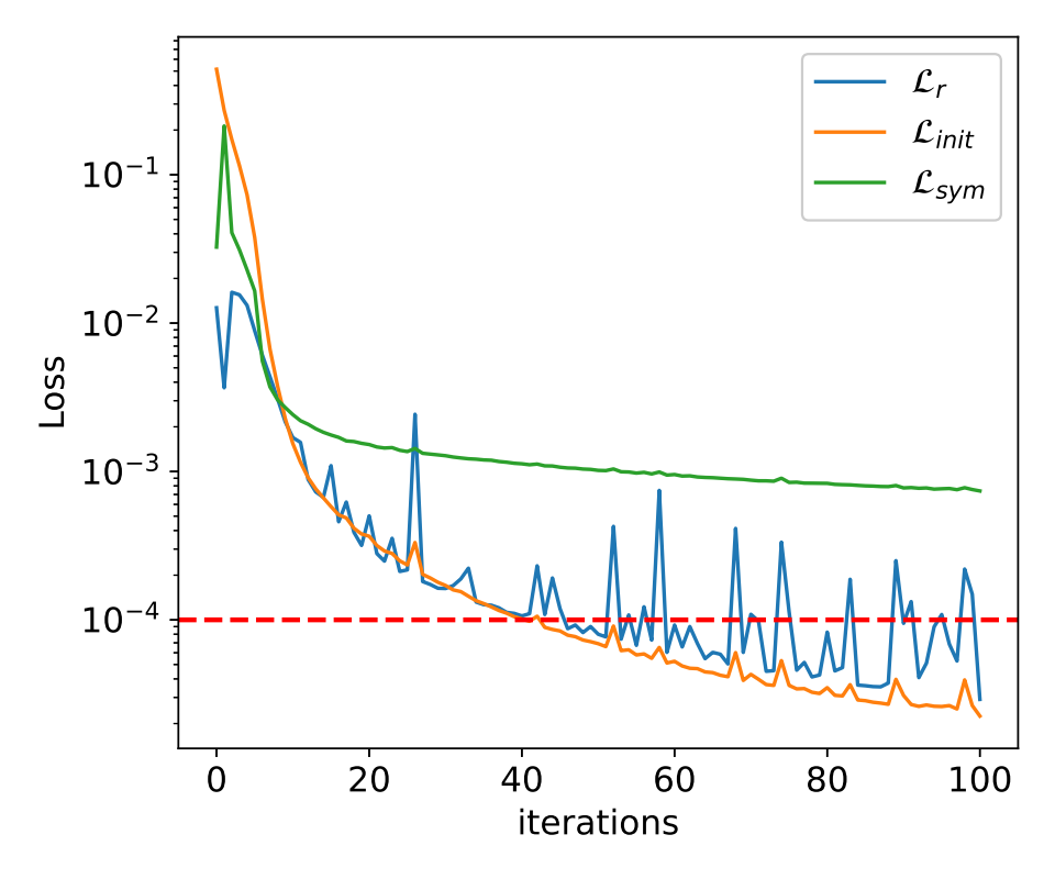
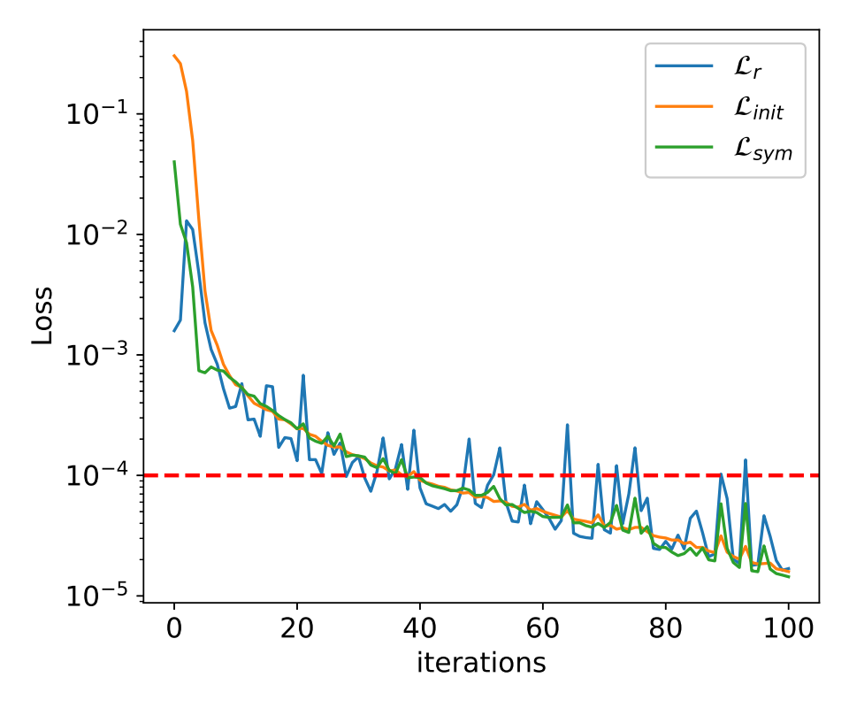
Figure 1: Loss value of vanilla PINN (left) and GsPINN(right).

Fig. 1 provides the information of three different part of loss. It can be seen that with the help of GsPINN, new type of loss involved symmetry decreases quickly and finally attain the lower value. In table 1, we take a systematical simulation and compare vanilla PINN and GsPINN about different part of loss precision under different set of collocation points. Table reflects the important role of GsPINN which can significantly save computational time however enhance the accuracy at the same time. Fig 2 illustrate the numerical solution at a time slot and comparison with standard solution. It can be directly seen that the enhancement of precision of solution.

Table 1: Influence of number in collocation points. Adam(3000) + L-BFGS, Loss weights $\lambda_{i}=\lambda_{r}=\lambda_{s}=1.0$

Algorithm	Loss(MSE)	Loss(init)	Loss(res)	Loss(sym)	time	points($[N_{i},N_{r},N_{s}]$)
PINN	2.276e-01	3.707e-03	6.591e-03	/	401.3667	[500, 5000, 0]
GsPINN	1.045e-01	3.100e-03	8.831e-03	5.182e-03	390.2504	[500, 5000, 1000]
GsPINN	1.305e-01	3.081e-03	6.723e-03	4.560e-03	430.4121	[500, 5000, 3000]
GsPINN	4.874e-02	4.225e-03	8.348e-03	4.944e-03	365.6366	[500, 5000, 5000]
GsPINN	3.926e-02	3.125e-03	1.235e-02	1.014e-02	441.9190	[500, 3000, 5000]
GsPINN	4.815e-02	2.293e-03	4.356e-03	5.749e-03	929.7770	[500, 1000, 5000]
PINN	5.644e-02	7.772e-03	1.086e-02	/	568.9507	[500, 10000, 0]
GsPINN	5.747e-02	7.315e-03	1.883e-02	8.217e-03	338.3280	[500, 10000, 3000]
GsPINN	5.300e-02	5.599e-03	1.078e-02	5.001e-03	543.5857	[500, 10000, 5000]
GsPINN	5.833e-02	8.479e-03	1.862e-02	9.948e-03	395.3139	[500, 10000, 10000]
GsPINN	4.462e-02	3.680e-03	1.013e-02	5.638e-03	377.0454	[500, 5000, 10000]
GsPINN	5.591e-02	5.416e-03	1.067e-02	1.001e-02	514.2763	[500, 3000, 10000]
PINN	5.154e-02	5.968e-03	7.893e-03	/	611.5450	[1000, 5000, 0]
GsPINN	6.157e-02	7.576e-03	2.321e-02	1.047e-02	353.1501	[1000, 5000, 3000]
GsPINN	5.103e-02	1.144e-02	1.546e-02	9.443e-03	459.8366	[1000, 5000, 5000]
GsPINN	7.734e-02	8.695e-03	1.891e-02	1.468e-02	271.8132	[1000, 3000, 5000]
PINN	5.769e-02	6.024e-03	9.643e-03	/	515.7466	[1000, 10000, 0]
GsPINN	5.214e-02	3.316e-03	9.702e-03	5.650e-03	469.6560	[1000, 10000, 3000]
GsPINN	7.774e-02	9.573e-03	2.197e-02	1.276e-02	381.6296	[1000, 10000, 5000]
GsPINN	5.760e-02	5.683e-03	8.852e-03	4.347e-03	551.7782	[1000, 10000, 10000]
GsPINN	6.737e-02	1.526e-02	3.886e-02	2.310e-02	444.1592	[1000, 5000, 10000]
GsPINN	7.119e-02	5.198e-03	1.143e-02	9.559e-03	553.8613	[1000, 3000, 10000]

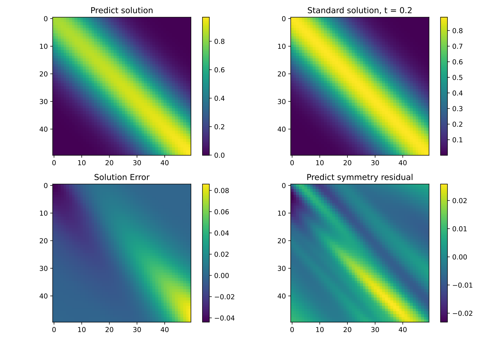
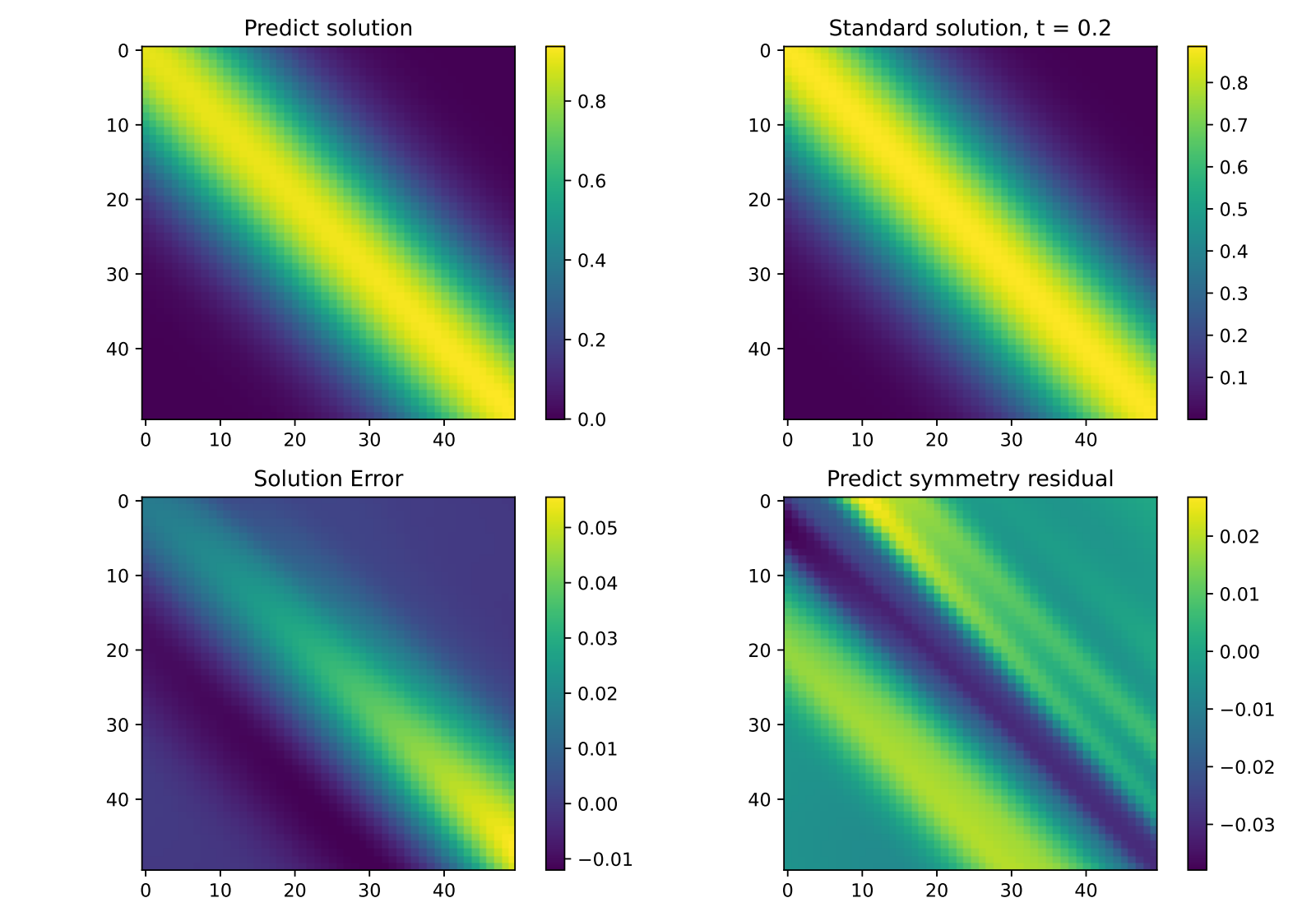
Figure 2: Comparison between exact solution and PINN solution. Left for vanilla PINN and right for GsPINN.

Example 4.2. Spatially varying diffusion equation is defined as the following:

$$\frac{\partial u}{\partial t}(t,x)=x\frac{\partial^{2}u}{\partial x^{2}}(t,x)+b\frac{\partial u}{\partial x}(t,x),\quad(t,x)\in[0,T]\times\mathbb{R}_{+}$$ (36)

where diffusion coefficient $b$ is set 0.5. Domain of spatial-temporal variable $(t,x)$ is $[0,T]\times\mathbb{R}_{+}$. $u:[0,T]\times\mathbb{R}_{+}\to\mathbb{R}$ is the desired solution. It is easy to find diffusion equation above is linear so it is associated to a fundamental solution.

$$\frac{\partial K}{\partial t}(t,x;y)=x\frac{\partial^{2}K}{\partial x^{2}}(t,x;y)+\frac{1}{2}\frac{\partial K}{\partial x}(t,x;y)$$ (37)

$$K(0,x;y)=\delta(x-y)$$

where $K:[0,T]\times\mathbb{R}_{+}\times\mathbb{R}_{+}\to\mathbb{R}$ is fundamental solution. The initial condition is set as delta function which can be regarded as a point source.

This Cauchy problem admits the explicit solution:

$$K(t,x;y)=\frac{1}{\sqrt{\pi ty}}\exp\left(-\frac{x+y}{t}\right)\cosh\left(\frac{2\sqrt{xy}}{t}\right)$$ (38)

By applying Lie symmetry method, the following infinitesimal generator can be verified to keep initial manifold and delta function invariant.

$$v=t^{2}\partial_{t}+2tx\partial_{x}-(x-y+bt)u\partial_{u}$$ (39)

Therefore invariant principle implies that the fundamental solution will have the symmetry invariant.

$$\left(x-y+\frac{1}{2}t\right)K(t,x,y)+t^{2}\frac{\partial K}{\partial t}(t,x,y)+2tx\frac{\partial K}{\partial x}(t,x,y)=0$$ (40)

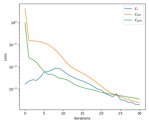
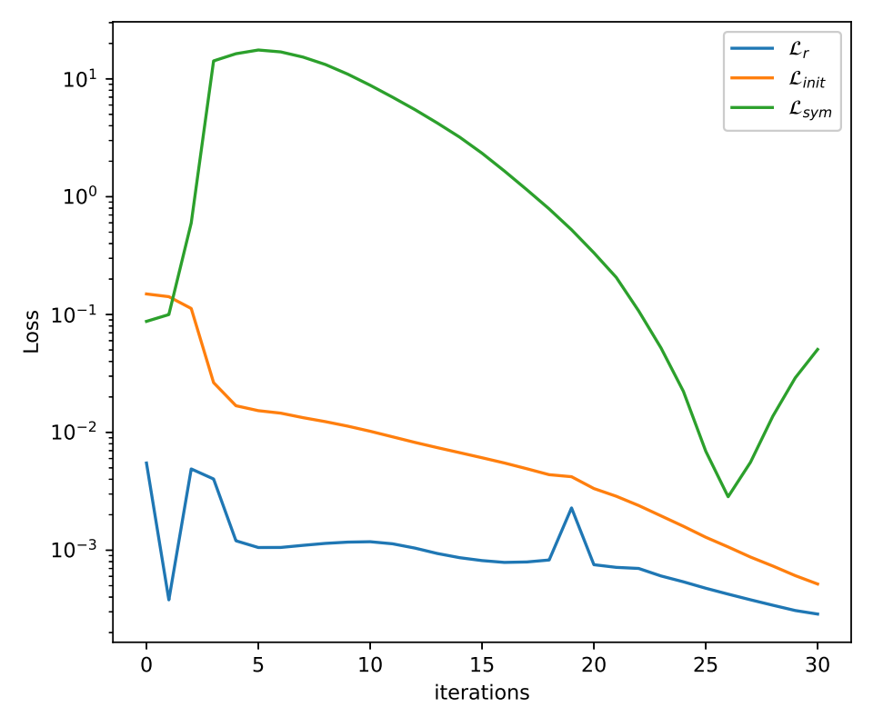
Figure 3: Loss value of PINN and GsPINN.

Table 2: Influence of number in collocation points. Adam(3000) + L-BFGS, Loss weights $\lambda_{i}=\lambda_{r}=\lambda_{s}=1.0$

Algorithm	Loss(MSE)	Loss(init)	Loss(res)	Loss(sym)	time	points($[N_{i},N_{r},N_{s}]$)
PINN	4.088e-01	6.331e-03	9.223e-03	/	222.7434	[200, 1000, 0]
GsPINN	4.904e-01	7.007e-03	1.207e-02	6.570e-03	189.4520	[200, 1000, 500]
GsPINN	4.382e-01	3.366e-03	4.930e-03	5.875e-03	393.1910	[200, 1000, 1000]
PINN	5.754e-02	2.057e-03	2.060e-03	/	419.1970	[500, 1000, 0]
GsPINN	4.694e-01	5.474e-03	7.666e-03	7.024e-03	293.4879	[500, 1000, 500]
GsPINN	5.212e-01	9.627e-03	9.451e-03	1.112e-02	246.4246	[500, 1000, 1000]
PINN	7.123e-02	3.051e-03	6.483e-03	/	511.9618	[500, 3000, 0]
GsPINN	5.975e-02	8.357e-03	1.656e-02	1.070e-02	342.3376	[500, 3000, 1000]
GsPINN	6.230e-02	7.124e-03	1.387e-02	1.128e-02	454.2537	[500, 3000, 3000]
GsPINN	5.758e-01	6.859e-03	7.860e-03	8.636e-03	374.3755	[500, 1000, 3000]
PINN	5.944e-02	1.955e-03	3.397e-03	/	657.7293	[500, 5000, 0]
GsPINN	6.309e-02	9.377e-03	2.127e-02	1.300e-02	290.7126	[500, 5000, 1000]
GsPINN	6.734e-02	4.672e-03	1.499e-02	1.111e-02	403.1887	[500, 5000, 3000]
GsPINN	6.116e-02	5.645e-03	1.238e-02	1.163e-02	428.6644	[500, 5000, 5000]
GsPINN	6.058e-02	9.191e-03	1.572e-02	1.307e-02	357.5372	[500, 3000, 5000]
GsPINN	4.731e-01	9.725e-03	1.009e-02	9.704e-03	324.4191	[500, 1000, 5000]
PINN	6.010e-02	3.470e-03	5.736e-03	/	581.2354	[500, 10000, 0]
GsPINN	5.907e-02	1.010e-02	1.916e-02	1.208e-02	386.7697	[500, 10000, 3000]
GsPINN	5.943e-02	1.000e-02	1.879e-02	1.252e-02	413.6504	[500, 10000, 5000]
GsPINN	6.056e-02	8.227e-03	1.904e-02	1.187e-02	454.1149	[500, 10000, 10000]
GsPINN	6.331e-02	7.220e-03	1.590e-02	1.237e-02	372.9199	[500, 5000, 10000]
GsPINN	6.045e-02	9.183e-03	1.639e-02	1.095e-02	7507.7460	[500, 3000, 10000]
PINN	6.203e-02	2.853e-03	4.931e-03	/	502.8584	[1000, 5000, 0]
GsPINN	6.360e-02	1.035e-02	2.228e-02	1.180e-02	247.0146	[1000, 5000, 3000]
GsPINN	6.373e-02	7.050e-03	1.709e-02	1.155e-02	313.9919	[1000, 5000, 5000]
GsPINN	6.832e-02	7.936e-03	1.542e-02	1.270e-02	454.1938	[1000, 3000, 5000]
PINN	6.578e-02	3.222e-03	5.807e-03	/	625.3559	[1000, 10000, 0]
GsPINN	6.008e-02	1.140e-02	2.037e-02	1.275e-02	350.9773	[1000, 10000, 3000]
GsPINN	5.820e-02	8.360e-03	1.900e-02	1.141e-02	398.2439	[1000, 10000, 5000]
GsPINN	5.958e-02	6.863e-03	1.619e-02	1.129e-02	601.7399	[1000, 10000, 10000]
GsPINN	6.319e-02	6.208e-03	1.201e-02	1.080e-02	407.6808	[1000, 5000, 10000]
GsPINN	6.267e-02	7.309e-03	1.468e-02	1.019e-02	388.8910	[1000, 3000, 10000]

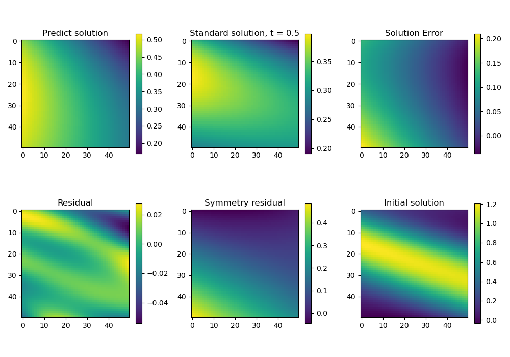
Figure 4: Comparison between exact solution and PINN solution.

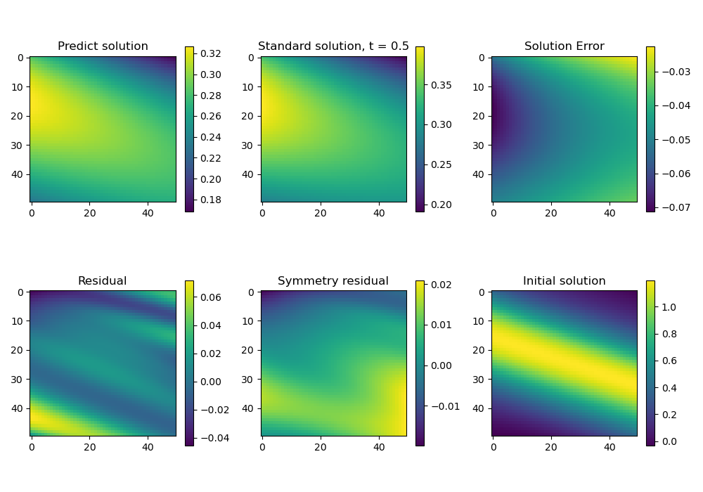
Figure 5: Comparison between exact solution and GSPINN solution.

Fig. 3 displays the loss components across three distinct categories. The graph indicates that with the inclusion of GsPINN, the novel symmetry-related loss decreases rapidly and reaches a lower value compared to others. Table 2 systematically compares the precision of loss components between vanilla PINN and GsPINN under varying collocation points. The table highlights GsPINN’s effectiveness in significantly reducing computational time while simultaneously improving accuracy. Fig. 4 and 5 depict the numerical solutions at a specific time step alongside the standard solution. The figures clearly demonstrate the enhanced precision achieved by our method.

5 Appendix

5.1 Additional background of group theory

Next we shall introduce some elementary knowledge about group theory and Lie algebra theory. In order to be suitable for more general readers, concrete examples will be illustrated under each abstract definition.

As a beginning, abstract formulation of group will be given as a most fundamental concept.

Definition 5.1 (Group)

A group $G$ is a set equipped with an binary operation $\circ:G\times G\to G$ satisfying following property:

1. (identity) There exists identity element $e$ such that $e\circ g=g\circ e=g$ holds for any $g\in G$.

2. (associativity) For any elements $g,h,w\in G$, $(g\circ h)\circ w=g\circ(h\circ w)$ holds.

3. (inverse) For any element $g\in G$, there exists element $g^{-1}\in G$ satisfying $g\circ g^{-1}=g^{-1}\circ g=e$.

Example 5.1

The most common cases of group include $(\mathbb{Z},+),(\mathbb{Q}\backslash\{0\},*)$.

Definition 5.2 (Lie group)

A Lie group is a smooth manifold associated with a group structure such that group operations are smooth. More precisely, group multiplication $\circ:G\times G\to G$ and inversion mapping are needed to be differentiable.

Example 5.2

Consider $GL(n,\mathbb{R})$ is the set of all inversible matrice of size $n\times n$ equipped with usual matrix multiplication. Notice that each component of multiplcation and inversion are all differentiable so that $(GL(n,\mathbb{R}),\circ)$ is a Lie group.

Definition 5.3 (Group action)

Let $G$ be a Lie group. A group action is defined as a mapping $\cdot:G\times M\to M$ on manifold $M$ which satisfies

1. (Identity) $e\cdot a=a$ holds for any $a\in M$.

2. (Compatibility) $g\cdot(h\cdot a)=(g\circ h)\cdot a$ holds for any $g,h\in G$ and $a\in M$.

Next we give some basic concepts related to Lie algebra.

Definition 5.4

If $X$ and $Y$ are differential operators, the Lie bracket of $X$ and $Y$, $[X,Y]$, is defined by $[X,Y]\phi=X(Y\phi)-Y(X\phi)$ for any $C^{\infty}$ function $\phi$.

Definition 5.5

A vector space $\mathcal{F}$ with the Lie bracket operation $\mathcal{F}\times\mathcal{F}\rightarrow\mathcal{F}$ denoted by $(x,y)\longmapsto[x,y]$ is called a Lie algebra if the following axioms are satisfied

(1) The Lie bracket operation is bilinear;

(2) $[x,x]=0$ for all $x\in\mathcal{F}$;

(3) $[x,[y,z]]+[y,[z,x]]+[z,[x,y]]=0,\quad x,y,z\in\mathcal{F}$.

5.2 Lie symmetry method

Lie group, as a powerful tool in mathematics, originated from the study of symmetric property of solution set, especially for solution of PDE. We shall consider a general form PDE system $\mathcal{L}(x,u)=0$ with its solution space denoted as $\text{Sol}(\mathcal{L})$. Here $x\in\mathbb{R}^{p}$ is independent coordinates, $u=u(x)$ is the unique solution and $\mathcal{L}$ represents a differential operator.

Reformulation of PDE system In the following, another viewpoint of PDE will be introduced with assumption of order $n$. First in order to describe all derivative variables of solution, jet space $J^{(n)}$ is introduced as $J^{(n)}:=X\times U\times U_{1}\times\cdots\times U_{n}$. Here $X=\mathbb{R}^{p}$ is domain of independent variable $x$, and

$$U_{i}:=\left\{\frac{\partial^{i}u}{\partial x_{j_{1}}\partial x_{j_{2}}\cdots\partial x_{j_{p}}}:j_{1}+j_{2}+\cdots j_{p}=i\right\}$$

represent set of all $i$-order partial derivative.

Therefore, solution space $\text{Sol}(\mathcal{L})$ can be understood as a subvariety $S_{\Delta}:=\{(x,u^{(n)})\in J^{(n)}:\mathcal{A}(x,u^{(n)})=0\}$, where $\mathcal{A}:J^{(n)}\to\mathbb{R}$ is a smooth function mapping. A simple example can be shown if considering Laplace equation $u_{x_{1}x_{1}}+u_{x_{2}x_{2}}=0$ with independent variable space $\mathbb{R}^{2}$. Correspondingly independent variable $x=(x_{1},x_{2})$, and jet expansion of dependent variable $u^{(2)}=(u,u_{x_{1}},u_{x_{2}},u_{x_{1}x_{1}},u_{x_{1}x_{2}},u_{x_{2}x_{2}})\in\mathbb{R}^{6}$. Smooth mapping $\mathcal{A}:(x,u^{(2)})\mapsto u_{x_{1}x_{1}}+u_{x_{2}x_{2}}$ is an affine function. Next in order to describe symmetric transformation, symmetry group is introduced.

Definition 5.6 (Symmetry group)

A symmetry group related to PDE system refers to a local group action $G\curvearrowright X\times U$ which satisfies for any $g\in G$, $u=g\cdot f\in\text{Sol}(\mathcal{A})$ if $u=f(x)\in\text{Sol}(\mathcal{A})$. Elements in symmetry group are usually called transformations.

It is noted that a transformation has nothing to do with derivative of a solution $f$. In order to extend the action to the jet space, we shall introduce a concept of prolongation. First of all, the following simple example is shown to illustrate the transformation on a concrete function.

Example 5.3

Consider Lie group $SO(2)$ describing the set of rotation matrice of size $2\times 2$. The function mentioned here is an affine polynomial $u=ax+b$. Next transformed function with a rotation $\theta$ can be written down

$$\tilde{u}=\frac{\sin\theta+a\cos\theta}{\cos\theta-a\sin\theta}\tilde{x}+\frac{b}{\cos\theta-a\sin\theta}$$ (41)

The notion of prolongation is motivated by extending the domain of a group action such that we can simultaneously make transformation of tangent space.

Definition 5.7 (Prolongation of Group action)

let $M$ be an open set in $X\times U$ and $M^{(n)}:=M\times U_{1}\times\cdots\times U_{n}$. Given a function $u=u(x)$ with corresponding graph defined in $M$, the prolongation of group transformation $g$ is defined as

$$\text{pr}^{(n)}g\cdot(x,u^{(n)}):=(\tilde{x},\tilde{u}^{(n)})$$ (42)

where

$$\tilde{u}^{(n)}:=\text{pr}^{(n)}(g\cdot u)(\tilde{x})$$ (43)

From the above definition, prolongation of group action is based on the prolongation of a single function. The main consideration lies in first applying $g$ to transform the function $u$ then obtaining derivative from new transformed function at the point $\tilde{x}$.

After finishing the prolongation of group action, corresponding infinitesimal generator can be also prolonged to high order jet space. Let $v$ be a infinitesimal generator defined on $M\subset X\times U$ with one-parameter flow $\exp(\varepsilon v)$. Infinitesimal generators we considered here are all differentiable. This leads to an equivalent relation between infinitesimal generator and one-parameter flow. The motivation here is any smooth infinitesimal generator $v$ will induce a differentiable flow $\psi(\epsilon,x)=\exp(\epsilon v)x$ in which group action $\exp(\epsilon v)$ can be detached simultaneously. One-parameter group action can be prolonged by applying method defined in Definition 5.7. This new prolonged action will correspond to a new flow followed by a new prolonged infinitesimal generator $\text{pr}^{(n)v}$, i.e.,

$$pr^{(n)}v=\frac{d}{d\varepsilon}\Big{|}_{\varepsilon=0}pr^{(n)}\exp(\varepsilon v)(x,u^{(n)})$$ (44)

In practice, general prolongation formula can be applied to extend infinitesimal generator to arbitrary order. For the sake of simplicity, we shall only consider the case of $q=1$.

Proposition 5.2.1 (General prolongation)

Let

$$v=\sum_{i=1}^{p}\xi^{i}(x,u)\partial_{x_{i}}+\phi(x,u)\partial_{u}$$ (45)

be a zero-order infinitesimal generator. Its corresponding prolongation of order $n$ can be written as

$$pr^{(n)}v=v+\sum_{|J|\leq n}\phi^{J}(x,u^{(n)})\partial_{u_{J}}$$ (46)

where component $\phi^{J}(x,u^{(n)})=D_{J}(\phi-\sum_{i=1}^{p}\xi^{i}\partial_{x_{i}}(u))+\sum_{i=1}^{p}\xi^{i}\partial_{x_{i}}(u_{J})$, $D_{J}$ denotes total derivative.

Difference between partial and total derivative.

Example 5.4

Let infinitesimal generator defined as $v=-u\partial_{x}+x\partial_{u}$ with corresponding $\xi=-u$ and $\phi=x$. By general prolongation formula, $pr^{(2)}v=v+\phi^{x}\partial_{u_{x}}+\phi^{xx}\partial_{u_{xx}}$ where components $\phi^{x},\phi^{xx}$ are calculated as below,

$$\phi^{x}= D_{x}(x+uu_{x})-uu_{xx}$$ (47)

$$= 1+u_{x}^{2}+uu_{xx}-uu_{xx}$$

$$= 1+u_{x}^{2}$$

and

$$\phi^{xx}= D_{xx}(x+uu_{x})+(-u)u_{xxx}$$ (48)

$$= D_{x}(1+u_{x}^{2}+uu_{xx})-uu_{xxx}$$

$$= 3u_{x}u_{xx}$$

Up to now, we can calculate prolonged infinitesimal generator of arbitrary order which can allow us to obtain following linearized symmtry condition (LSC).

Definition 5.8

For a prolonged infinitesimal generator

$$X=\xi\partial_{x}+\tau\partial_{t}+\eta\partial_{u}+\eta^{x}\partial_{u_{x}}+\eta^{t}\partial_{u_{t}}+\cdots$$ (49)

Linearized symmetry condition states $X(\mathcal{A}(x,u^{(n)}))$ will vanish at the solution set $\mathcal{A}(x,u^{(n)})=0$, i.e.,

$$X(\mathcal{A}(x,u^{(n)}))=0,\quad\text{when }\mathcal{A}(x,u^{(n)})=0$$ (50)

Solving LSC will yield a set of linearly independent infinitesimal generators $\{v_{i}\},i\geq 1$ which span a Lie algebra named symmetry algebra. There is a one-to-one correspondence between symmetry algebra and symmetry group.

5.3 Proof

Here, some detailed proof will be provided.

C1. Proof of Theorem 3.1.

Notice that the initial manifold here is $S=\{t=0\}\times\mathbb{R}$. First requirement of invariance principle is that $v(t)\Big{|}_{S}=0$, where $(\cdot)$ means a functional action over function $t$. It implies component should be satisfied by $\tau(0,x,u)=0$. Followed by this requirement, infinitesimal generator $\mathbf{v}$ restricted on initial manifold will become

$$\mathbf{v}\Big{|}_{S}=\xi(0,x,u)\partial_{x}+\eta(0,x,u)\partial_{u}$$ (51)

The second requirement of invariance principle is stated as $\mathbf{v}\Big{|}_{S}(u-f)\Big{|}_{u=f}=0$. By definition of infinitesimal transformation, we shall derive $\bar{x}=x+a\xi(0,x,u)+\mathcal{O}(a^{2})$ and $\bar{u}=u+a\eta(0,x,u)+\mathcal{O}(a^{2})$. By utilizing Lemma 3.1.1, initial distribution will be transformed as $\bar{f}=f-a\xi_{x}(0,x,u)\cdot f$. It will yield that

$$\mathbf{v}\Big{|}_{S}(u-f)\Big{|}_{u=f} =\mathbf{v}\Big{|}_{S}(u)\Big{|}_{u=f}-\mathbf{v}\Big{|}_{S}(f)\Big{|}_{u=f}$$ (52)

$$=[\bar{u}-\bar{f}]\Big{|}_{u=f}$$

$$=a[(\eta(0,x,u)+\xi_{x}(0,x,u)\cdot f)]\Big{|}_{u=f}+\mathcal{O}(a^{2})$$

$$=a[\eta(0,x,f(x))+\xi_{x}(0,x,f(x))\cdot f(x)]+\mathcal{O}(a^{2})$$

Finally, $\mathbf{v}\Big{|}_{S}(u-f)$ vanishes at the $u=f$ is equivalent to $\eta(0,x,f(x))+\xi_{x}(0,x,f(x))\cdot f(x)=0$ for $x\in\mathbb{R}$.

Finally it should be noted that symmetry group should keep support of initial distribution unchanged to satisfy the invariance principle. Considering generator

$$v\Big{|}_{t=0}=\xi(0,x,u)\partial_{x}+\eta(0,x,u)\partial_{u}$$ (53)

is corresponding to transformation $g:\mathbb{R}\to\mathbb{R}$ by $x\mapsto\bar{x}$ under infinitesimal transformation. Invariance of support is equivalent to $g(supp(f))\subset supp(f)$, i.e.,

$$x+a\xi(0,x,u)\in supp(f),\ \text{if}\ x\in supp(f)$$ (54)

$\square$

C2. Proof of Theorem 3.2.

By applying Theorem 3.1, we can easily obtain $\tau(0,x)=0$ from the first equation (19). Furthermore, starting from second identity of (19),

$$\eta(0,x,f(x))+\xi_{x}(0,x)\cdot f(x) =\phi(0,x)f(x)+\xi_{x}(0,x)\cdot f(x)$$ (55)

$$=[\phi(0,x)+\xi_{x}(0,x)]f(x)$$

$$=0$$

the above identity implies the desired result. $\square$

C3. Proof of Theorem 3.3.

The only thing we need to do is to replace $f(x)$ with $\delta(x-y)$ and notice $\text{supp}(\delta)=\{x=y\}$. Results of Theorem 3.2 correspond to the following

$$\begin{cases}\tau(0,x;y)=0\\ [\phi(0,x;y)+\xi_{x}(0,x;y)]\Big{|}_{\text{supp}(\delta)}=0\end{cases}$$ (56)

where $y$ should be regarded as an external parameter. $\square$

C4. Derivation of symmetric condition for heat equation

Recall the heat equation,

$$u_{t}-u_{xx}=0$$ (57)

The corresponding symmetry group can be obtained by routing procedure mentioned in previous section.

$$\mathbf{v}_{0}=\partial_{t},\quad\mathbf{v}_{1}=\partial_{x},$$ (58)

$$\mathbf{v}_{2}=2t\partial_{t}+x\partial_{x},\quad\mathbf{v}_{3}=u\partial_{u},\quad\mathbf{v}_{4}=2t\partial_{x}-xu\partial_{u}$$

$$\mathbf{v}_{5}=t^{2}\partial_{t}+tx\partial_{x}-\frac{1}{4}(2nt+x^{2})u\partial_{u}$$

Theorem 5.5

The following operator $\mathbf{v}_{2}-n\mathbf{v}_{3}+y\mathbf{v}_{1}$ is a invariant transformation admitted by Cauchy problem

$$\frac{\partial K}{\partial t}(t,x;y)=\frac{\partial^{2}K}{\partial x^{2}}(t,x;y)$$ (59)

$$K(0,x;y)=\delta(x-y),\quad(x,y)\in\mathbb{R}\times\mathbb{R}$$

Proof 5.6.

The only thing we need to do is to verify the condition of Theorem 3.3. First we notice that both operators $\mathbf{v}_{2},\mathbf{v}_{3}$ do not satisfy the invariant condition mentioned in Theorem 3.3. In the following, we shall consider the new combination:

$$\mathbf{v}_{2}-n\mathbf{v}_{3}+y\mathbf{v}_{1}=2t\partial_{t}+(x+\tilde{\lambda})\partial_{x}+\lambda u\partial_{u}$$ (60)

In this example, there are the following correspondence

$$\tau(t,x;y)= 2t$$ (61)

$$\xi(t,x;y)= x+\tilde{\lambda}$$

$$\phi(t,x;y)= \lambda$$

Direct computation implies that

$$\tau(0,x;y)\equiv 0$$ (62)

and

$$[\phi(0,x;y)+\xi_{x}(0,x;y)]\Big{|}_{x=y}=\lambda+\nabla_{x}(x)=\lambda+n$$ (63)

and

$$\xi(0,y;y)=y+\tilde{\lambda}$$ (64)

Theorem 3.3 will hold if and only if $\lambda=-n$ and $\tilde{\lambda}=-y$ that is the desired result.

C5. Derivation of symmetric condition for diffusion equation

Recall the diffusion equation

$$u_{t}=xu_{xx}+bu_{x},\quad b>0$$ (65)

The corresponding symmetry group can be obtained by routing procedure mentioned in previous section.

$$\mathbf{v}_{0}=u\partial_{u},\quad\mathbf{v}_{1}=\partial_{t},\quad\mathbf{v}_{2}=t\partial_{t}+x\partial_{x}$$ (66)

$$\mathbf{v}_{3}=t^{2}\partial_{t}+2tx\partial_{x}-(x+bt)u\partial_{u}$$

Theorem 5.7.

The following operator $\mathbf{v}_{3}+\lambda\mathbf{v}_{0}$ is a invariant transformation admitted by Cauchy problem

$$\frac{\partial K}{\partial t}(t,x;y)=x\frac{\partial^{2}K}{\partial x^{2}}(t,x;y)+\frac{1}{2}\frac{\partial K}{\partial x}(t,x;y)$$ (67)

$$K(0,x;y)=\delta(x-y)$$

Proof 5.8.

The only thing we need to do is to verify the condition of Theorem 3.3. First we notice that both operators $\mathbf{v}_{0}$ and $\mathbf{v}_{3}$ do not satisfy the invariance condition mentioned in Theorem 3.3. In the following, we shall consider the new combination:

$$\mathbf{v}_{3}+\lambda\mathbf{v}_{0}=t^{2}\partial_{t}+2tx\partial_{x}-(x+bt-\lambda)u\partial_{u}$$ (68)

In this example, there are the following correspondence

$$\tau(t,x;y)=t^{2}$$ (69)

$$\xi(t,x;y)=2tx$$

$$\phi(t,x;y)=-(x+bt-\lambda)$$

Direct computation implies that

$$\tau(0,x;y)\equiv 0$$ (70)

and

$$[\phi(0,x;y)+\xi_{x}(0,x;y)]\Big{|}_{x=y}=[-(x-\lambda)]\Big{|}_{x=y}=\lambda-y$$ (71)

and

$$\xi(0,x;y)=0$$ (72)

Theorem 3.3 will hold if and only if $\lambda=y$ that is the desired result.

References

References

- [1] Tara Akhound-Sadegh, Laurence Perreault-Levasseur, Johannes Brandstetter, Max Welling, and Siamak Ravanbakhsh. Lie point symmetry and physics-informed networks. Advances in Neural Information Processing Systems, 36, 2024.
- [2] Sokratis J Anagnostopoulos, Juan Diego Toscano, Nikolaos Stergiopulos, and George Em Karniadakis. Residual-based attention in physics-informed neural networks. Computer Methods in Applied Mechanics and Engineering, 421:116805, 2024.
- [3] Anima Anandkumar, Kamyar Azizzadenesheli, Kaushik Bhattacharya, Nikola Kovachki, Zongyi Li, Burigede Liu, and Andrew Stuart. Neural operator: Graph kernel network for partial differential equations. In ICLR 2020 Workshop on Integration of Deep Neural Models and Differential Equations, 2020.
- [4] Ricardo Cortez. The method of regularized stokeslets. SIAM Journal on Scientific Computing, 23(4):1204–1225, 2001.
- [5] Nail’Khairullovich Ibragimov. A Practical Course in Differential Equations and Mathematical Modelling: Classical and New Methods, Nonlinear Mathematical Models, Symmetry and Invariance Principles. World Scientific, 2009.
- [6] Zongyi Li, Nikola Kovachki, Kamyar Azizzadenesheli, Burigede Liu, Kaushik Bhattacharya, Andrew Stuart, and Anima Anandkumar. Fourier neural operator for parametric partial differential equations. arXiv preprint arXiv:2010.08895, 2020.
- [7] Levi McClenny and Ulisses Braga-Neto. Self-adaptive physics-informed neural networks using a soft attention mechanism. arXiv preprint arXiv:2009.04544, 2020.
- [8] Peter J Olver. Applications of Lie groups to differential equations, volume 107. Springer Science & Business Media, 1993.
- [9] Maziar Raissi, Paris Perdikaris, and George E Karniadakis. Physics-informed neural networks: A deep learning framework for solving forward and inverse problems involving nonlinear partial differential equations. Journal of Computational physics, 378:686–707, 2019.
- [10] Sifan Wang, Shyam Sankaran, and Paris Perdikaris. Respecting causality for training physics-informed neural networks. Computer Methods in Applied Mechanics and Engineering, 421:116813, 2024.
- [11] Sifan Wang, Xinling Yu, and Paris Perdikaris. When and why pinns fail to train: A neural tangent kernel perspective. Journal of Computational Physics, 449:110768, 2022.
- [12] Liu Yang, Xuhui Meng, and George Em Karniadakis. B-pinns: Bayesian physics-informed neural networks for forward and inverse pde problems with noisy data. Journal of Computational Physics, 425:109913, 2021.
- [13] Bing Yu et al. The deep ritz method: a deep learning-based numerical algorithm for solving variational problems. Communications in Mathematics and Statistics, 6(1):1–12, 2018.
- [14] Zhi-Yong Zhang, Sheng-Jie Cai, and Hui Zhang. A symmetry group based supervised learning method for solving partial differential equations. Computer Methods in Applied Mechanics and Engineering, 414:116181, 2023.
- [15] Zhi-Yong Zhang, Hui Zhang, Li-Sheng Zhang, and Lei-Lei Guo. Enforcing continuous symmetries in physics-informed neural network for solving forward and inverse problems of partial differential equations. Journal of Computational Physics, 492:112415, 2023.
- [16] Zongren Zou, Xuhui Meng, and George Em Karniadakis. Correcting model misspecification in physics-informed neural networks (pinns). Journal of Computational Physics, 505:112918, 2024.
- [17] Zongren Zou, Xuhui Meng, Apostolos F Psaros, and George E Karniadakis. Neuraluq: A comprehensive library for uncertainty quantification in neural differential equations and operators. SIAM Review, 66(1):161–190, 2024.