Neural stochastic Volterra equations:
learning path-dependent dynamics

Abstract.

Stochastic Volterra equations (SVEs) serve as mathematical models for the time evolutions of random systems with memory effects and irregular behaviour. We introduce neural stochastic Volterra equations as a physics-inspired architecture, generalizing the class of neural stochastic differential equations, and provide some theoretical foundation. Numerical experiments on various SVEs, like the disturbed pendulum equation, the generalized Ornstein–Uhlenbeck process and the rough Heston model are presented, comparing the performance of neural SVEs, neural SDEs and Deep Operator Networks (DeepONets).

Key words: feedforward neural network, deep operator network, neural stochastic differential equation, stochastic Volterra equation, supervised learning.

MSC 2020 Classification: 62M45, 68T07, 60H20.

1. Introduction

Stochastic Volterra equations (SVEs) are used as mathematical models for the time evolutions of random systems appearing in various areas like biology, finance or physics. SVEs are a natural generalization of ordinary stochastic differential equations (SDEs) and, in contrast to SDEs, they are capable to represent random dynamics with memory effects and very irregular trajectories. For instance, SVEs are used in the modelling of turbulence [BNS08], of volatility on financial markets [EER19] and of DNA patterns [RBS10].

Combining differential equations and neural networks into hybrid approaches for statistical learning has been gaining increasing interest in recent years, see e.g. [E17, CRBD18]. This has led to many very successful data-driven methods to learn solutions of various differential equations. For instance, neural stochastic differential equations are SDEs with coefficients parametrized by neural networks, and serve as continuous-time generative models for irregular time series, see [LXS⁺19, LWCD20, KFLL21, IHLS24]. Models based on neural SDEs are of particular interest in financial engineering, see [CKT20, GSVS⁺22, CRW22]. Further examples of ‘neural’ differential equations are neural controlled differential equations [KMFL20], which led to very successful methods for irregular time series, neural rough differential equations [MSKF21], which are especially well-suited for long time series, and neural stochastic partial differential equations [SLG22], which are capable to process data from continuous spatiotemporal dynamics. Loosely speaking, ‘neural’ differential equations and their variants can be considered as continuous-time analogous to various recurrent neural networks.

In the present work, we introduce neural stochastic Volterra equations as stochastic Volterra equations with coefficients parameterized by neural networks. They constitute a natural generalization of neural SDEs with the advantage that they are capable to represent time series with temporal dependency structures, which overcomes a limitation faced by neural SDEs. Hence, neural SVEs are suitable to serve as generative models for random dynamics with memory effects and irregular behaviour, even more irregular than neural SDEs. As theoretical justification for the universality of neural SVEs, we provide a stability result for general SVEs in Proposition 2.3, which can be combined with classical universal approximation theorems for neural networks [Cyb89, Hor91].

Relying on neural stochastic Volterra equations parameterized by feedforward neural networks, we study supervised learning problems for random Volterra type dynamics. More precisely, we consider setups, where the training sets consist of sample paths of the ’true’ Volterra process together with the associated realizations of the driving noise and the initial condition, and build a neural SVEs based model aiming to reproduce the sample paths as good as possible. A related supervised learning problem in the context of stochastic partial differential equations (SPDEs) was treated in [SLG22] introducing neural SPDEs. For unsupervised learning problems using neural SDEs we refer to [Kid22].

We numerically investigate the supervised learning problem for prototypical Volterra type dynamics such as the disturbed pendulum equation [Øks03], the rough Heston model [EER19] and the generalized Ornstein–Uhlenbeck process [Vas12]. The performance of the neural SVE based models is compared to Deep Operator Networks (DeepONets) and to neural SDEs. Recall DeepONets are a popular class of neural learning algorithms for general operators on function spaces that were introduced in [LJP⁺21]. For the training process of the neural SVE we choose the Adam algorithm, as introduced in [KB14], which is known to be a well-suited stochastic gradient descent method for stochastic optimization problem.

The numerical study in Section 3 demonstrates that the presented neural SVE based methods outperform DeepONets significantly, see Table 1-Table 4. Especially, neural SVE based methods generalize much more efficiently as one can see at the good performance on the test sets, where neural SVEs are up to $20$ times more accurate than DeepONets. An advantage of neural SVEs are not only the physics-informed architecture, they are also time-resolution invariant, meaning that they can be trained and evaluated on arbitrary, possibly different time grid discretizations. Moreover, neural SVEs outperform neural SDE based models for random dynamics with a dependency structure, cf. Subsection 3.4.

Organization of the paper: In Section 2 we introduce neural stochastic Volterra equations and their theoretical background. The numerical experiments are presented in Section 3.

2. Neural stochastic Volterra equations

Let $(\Omega,\mathcal{F},(\mathcal{F}_{t})_{t\in[0,T]},\mathbb{P})$ be a filtered probability space, which satisfies the usual conditions, $T\in(0,\infty)$ and $d,m\in\mathbb{N}$. Given an $\mathbb{R}^{d}$-valued random initial condition $\xi$ and an $m$-dimensional standard Brownian motion $(B_{t})_{t\in[0,T]}$, we consider the $d$-dimensional stochastic Volterra equation (SVE)

(2.1) $$X_{t}=\xi\,g(t)+\int_{0}^{t}K_{\mu}(t-s)\mu(s,X_{s})\,\mathrm{d}s+\int_{0}^{t}K_{\sigma}(t-s)\sigma(s,X_{s})\,\mathrm{d}B_{s},\quad t\in[0,T],$$

where $g\colon[0,T]\to\mathbb{R}$ is a deterministic continuous function (where we usually normalize $g(0)=1$), the coefficients $\mu\colon[0,T]\times\mathbb{R}^{d}\to\mathbb{R}^{d}$ and $\sigma\colon[0,T]\times\mathbb{R}^{d}\to\mathbb{R}^{d\times m}$, and the convolutional kernels $K_{\mu},K_{\sigma}\colon[0,T]\to\mathbb{R}$ are measurable functions. Furthermore, $\int_{0}^{t}K_{\sigma}(t-s)\sigma(s,X_{s})\,\mathrm{d}B_{s}$ is defined as an Itô integral. We refer to [KS91, Øks03] for introductory textbooks on stochastic integration and to [PP90, CLP95, CD01] for classical results on SVEs.

To define the notion of a (strong) $L^{p}$-solution, let $L^{p}(\Omega\times[0,T])$ be the space of all real-valued, $p$-integrable functions on $\Omega\times[0,T]$. We call an $(\mathcal{F}_{t})_{t\in[0,T]}$-progressively measurable stochastic process $(X_{t})_{t\in[0,T]}$ in $L^{p}(\Omega\times[0,T])$ on the given probability space $(\Omega,\mathcal{F},(\mathcal{F}_{t})_{t\in[0,T]},\mathbb{P})$, a (strong) $L^{p}$-solution of the SVE (2.1) if $\int_{0}^{t}(|K_{\mu}(t-s)\mu(s,X_{s})|+|K_{\sigma}(t-s)\sigma(s,X_{s})|^{2})\,\mathrm{d}s<\infty$ for all $t\in[0,T]$ and the integral equation (2.1) hold $\mathbb{P}$-almost surely. As usual, a strong $L^{1}$-solution $(X_{t})_{t\in[0,T]}$ of the SVE (2.1) is often just called solution of the SVE (2.1).

2.1. Neural SVEs

To learn the dynamics of the SVE (2.1), that is, the corresponding operators $\xi$, $g$, $K_{\mu}$, $K_{\sigma}$, $\mu$ and $\sigma$, we rely on some neural network architecture. To that end, let for some latent dimension $d_{h}>d$,

$$L_{\theta}\colon\mathbb{R}^{d}\to\mathbb{R}^{d_{h}},\quad g_{\theta}\colon[0,T]\to\mathbb{R},\quad K_{\mu,\theta}\colon[0,T]\to\mathbb{R},\quad K_{\sigma,\theta}\colon[0,T]\to\mathbb{R},$$

$$\mu_{\theta}\colon[0,T]\times\mathbb{R}^{d_{h}}\to\mathbb{R}^{d_{h}},\quad\sigma_{\theta}\colon[0,T]\times\mathbb{R}^{d_{h}}\to\mathbb{R}^{d_{h}\times m},\quad\Pi_{\theta}\colon\mathbb{R}^{d_{h}}\to\mathbb{R}^{d}$$

be seven feedforward neural networks (see [YYK15, Section 3.6.1]) that are parameterized by some common parameter $\theta$. Note that $L_{\theta}$ lifts the given initial value to the latent space $\mathbb{R}^{d_{h}}$, $\Pi_{\theta}$ is the readout back from the latent space to the space $\mathbb{R}^{d}$, and the other networks try to imitate their respectives in equation (2.1), on the latent $d_{h}$-dimensional space.

Given the input data $\xi\in\mathbb{R}^{d}$ and $(B_{t})_{t\in[0,T]}\in C([0,T];\mathbb{R}^{m})$, $\mathbb{P}$-a.s., we introduce the neural stochastic Volterra equations

$$Z_{0} =L_{\theta}(\xi),$$

(2.2) $$Z_{t} =Z_{0}\,g_{\theta}(t)+\int_{0}^{t}K_{\mu,\theta}(t-s)\mu_{\theta}(s,Z_{s})\,\mathrm{d}s+\int_{0}^{t}K_{\sigma,\theta}(t-s)\sigma_{\theta}(s,Z_{s})\,\mathrm{d}B_{s},$$

$$X_{t} =\Pi_{\theta}(Z_{t}),\quad t\in[0,T].$$

The objective is to optimize $\theta$ as good as possible such that the generated paths are as close as possible to the given training paths. Therefore, one needs to solve a stochastic optimization problem at each training step. One typically chosen and well-suited stochastic gradient descent method for stochastic optimization problem is the Adam algorithm, introduced in [KB14]. The Adam algorithm is known to be computationally efficient, requires little memory, is invariant to diagonal rescaling of gradients and is well-suited for high-dimensional problems with regard to data/parameters.

Given a trained supervised model $(L_{\theta},K_{\mu,\theta},K_{\sigma,\theta},\mu_{\theta},\sigma_{\theta},\Pi_{\theta})$, we can evaluate the neural SVE (2.1) given the input data $(\xi,B)$ by using any numerical scheme for stochastic Volterra equations. For that purpose, we use the Volterra Euler–Maruyama scheme introduced in [Zha08] for the training procedure. Note that Lipschitz conditions on $\mu_{\theta}$ and $\sigma_{\theta}$ can be imposed by using, e.g., LipSwish, ReLU or tanh activation functions.

2.2. Neural network architecture

The structure of the neural SVE model (2.1) is analogously defined to the structure of neural stochastic differential equations, as introduced in [Kid22], and of neural stochastic partial differential equations, as introduced in [SLG22]. The $d_{h}$-dimensional process $Z$ represents the hidden state. We impose the readout $\Pi_{\theta}$ to get back to dimension $d$. The model has, at least if one considers a setting where the initial condition cannot be observed like an unsupervised setting, some minimal amount of architecture. It is in such a setting necessary to induce the lift $L_{\theta}$ and the randomness by some additional variable $\tilde{\xi}$ to learn the randomness induced by the initial condition $X_{0}=\Pi_{\theta}\big{(}L_{\theta}(\tilde{\xi})g_{\theta}(0)\big{)}$ (otherwise $X_{0}$ would not be random since it does not depend on the Brownian motion $B$). Moreover, the structure induced by the lift $L_{\theta}$ and the readout $\Pi_{\theta}$ is the natural choice to lift the $d$-dimensional SVE (2.1) to the latent dimension $d_{h}>d$.

We use LipSwish activation functions in any layer of any network. These were introduced in [CBDJ19] as $\rho(z)=0.909z\sigma(z)$, where $\sigma$ is the sigmoid function. Due to the constant $0.909$, LipSwish activations are Lipschitz continuous with Lipschitz constant one and smooth. Moreover, there is strong empirical evidence that LipSwish activations are very suitable for a variety of challenging approximation tasks, see [RZL17].

For a given latent dimension $d_{h}>d$, the lift $L_{\theta}$ is modeled as a linear $1$-layer network from dimension $d$ to $d_{h}$ without any additional hidden layer, and, as its counterpart, the readout $\Pi_{\theta}$ as a linear $1$-layer network from $d_{h}$ to $d$. The networks $K_{\mu,\theta},K_{\sigma,\theta}$ and $g_{\theta}$ are all designed as linear networks from dimension $1$ to $1$ with two hidden layers of size $d_{K}$ for some additional dimension $d_{K}>d$. Lastly, the network $\mu_{\theta}$ is defined as a linear network from dimension $1+d_{h}$ to $d_{h}$ with one hidden layer of size $d_{h}$ and the network $\sigma_{\theta}$ from $1+d_{h}$ to $d_{h}\cdot m$ with one hidden layer of size $d_{h}\cdot m$.

2.3. Stability for SVEs

The mathematical reason that neural stochastic Volterra equations provide a suitable structure for learning the dynamics of general SVEs is the universal approximation property of neural networks, see e.g. [Cyb89, Hor91], and the stability result for SVEs, presented in this subsetions. More precisely, our stability result yields that if we approximate the kernels and coefficients of an SVE sufficiently well, we get a good approximation of the solution by the respective approximating solutions. To formulate the stability result, we need the following definitions and assumptions.

For $p\geq 1$, the $L^{p}$-norm of a function $h\colon[0,T]\to\mathbb{R}$ is defined by

$$\|h\|_{p}:=\Big{(}\int_{0}^{T}|h(s)|^{p}\,\mathrm{d}s\Big{)}^{\frac{1}{p}},$$

and the $\sup$-norms for functions $f\colon[0,T]\times\mathbb{R}^{d}\to\mathbb{R}^{d}$ and $g\colon[0,T]\to\mathbb{R}^{d}$, respectively, are given by

$$\|f\|_{\infty}:=\sup_{t\in[0,T],x\in\mathbb{R}^{d}}|f(t,x)|\quad\text{and}\quad\|g\|_{\infty}:=\sup_{t\in[0,T]}|g(x)|.$$

As comparison to the SVE (2.1), we consider the SVE

(2.3) $$\tilde{X}_{t}=\xi\,\tilde{g}(t)+\int_{0}^{t}\tilde{K}_{\mu}(t-s)\tilde{\mu}(s,\tilde{X}_{s})\,\mathrm{d}s+\int_{0}^{t}\tilde{K}_{\sigma}(t-s)\tilde{\sigma}(s,\tilde{X}_{s})\,\mathrm{d}B_{s},\quad t\in[0,T],$$

where $\tilde{g}\colon[0,T]\to\mathbb{R}$ is a continuous function, the coefficients $\tilde{\mu}\colon[0,T]\times\mathbb{R}^{d}\to\mathbb{R}^{d}$ and $\tilde{\sigma}\colon[0,T]\times\mathbb{R}^{d}\to\mathbb{R}^{d\times m}$, and the convolutional kernels $\tilde{K}_{\mu},\tilde{K}_{\sigma}\colon[0,T]\to\mathbb{R}$ are measurable functions.

For the convolutional kernels, we make the following assumption.

Assumption 2.1.

Let $q,\tilde{q}>1$ and $p\geq 2$ be such that

(2.4) $$\frac{1}{p}+\frac{1}{q}=1\quad\text{and}\quad\frac{2}{p}+\frac{1}{\tilde{q}}=1.$$

Suppose that $\|K_{\mu}\|_{q}+\|\tilde{K}_{\mu}\|_{q}<\infty$, $\|K_{\sigma}\|_{2\tilde{q}}+\|\tilde{K}_{\sigma}\|_{2\tilde{q}}<\infty$, $\|\mu\|_{\infty}+\|\tilde{\mu}\|_{\infty}+\|\sigma\|_{\infty}+\|\tilde{\sigma}\|_{\infty}<\infty$ and $\|g\|_{\infty}+\|\tilde{g}\|_{\infty}<\infty$.

For the coefficients, we require the standard Lipschitz and linear growth conditions.

Assumption 2.2.

Let $\mu,\sigma,\tilde{\mu},\tilde{\sigma}\colon[0,T]\times\mathbb{R}\to\mathbb{R}$ be measurable functions such that:

1. $\mu,\sigma$ and $\tilde{\mu},\tilde{\sigma}$ are of linear growth, i.e. there is a constant $C_{\mu,\sigma}>0$ such that

   $$|\tilde{\mu}(t,x)|+|\tilde{\sigma}(t,x)|+|\mu(t,x)|+|\sigma(t,x)|\leq C_{\mu,\sigma}(1+|x|),$$

   for all $t\in[0,T]$ and $x\in\mathbb{R}$.

2. $\mu,\sigma$ and $\tilde{\mu},\tilde{\sigma}$ are Lipschitz continuous in the space variable uniformly in time, i.e. there is a constant $C_{\mu,\sigma}>0$ such that

   $$|\mu(t,x)-\mu(t,y)|+|\sigma(t,x)-\sigma(t,y)|\leq C_{\mu,\sigma}|x-y|\quad\text{and}$$

   $$|\mu(t,x)-\mu(t,y)|+|\sigma(t,x)-\sigma(t,y)|\leq C_{\mu,\sigma}|x-y|$$

   holds for all $t\in[0,T]$ and $x,y\in\mathbb{R}$.

Based on these assumptions, we obtain the following stability result.

Proposition 2.3.

Suppose Assumption 2.1, Assumption 2.2 and assume $\xi\in L^{p}(\Omega)$. Let $(X_{t})_{t\in[0,T]}$ and $(\tilde{X}_{t})_{t\in[0,T]}$ be the solutions to the SVEs (2.1) and (2.3), respectively. Then, there is some constant $C>0$, depending on $\mu,\sigma,\tilde{\mu},\tilde{\sigma},{K}_{\mu},{K}_{\sigma},\tilde{K}_{\mu},\tilde{K}_{\sigma},p,\xi$, such that

(2.5) $$\sup_{t\in[0,T]}\mathbb{E}[|X_{t}-\tilde{X}_{t}|^{p}]\leq C\Big{(}\|g-\tilde{g}\|_{\infty}^{p}+\|\mu-\tilde{\mu}\|_{\infty}^{p}+\|\sigma-\tilde{\sigma}\|_{\infty}^{p}+\|K_{\mu}-\tilde{K}_{\mu}\|_{2\tilde{q}}^{p}+\|K_{\sigma}-\tilde{K}_{\sigma}\|_{2\tilde{q}}^{p}\Big{)}.$$

Proof.

First notice that, due to Assumption 2.1 and Assumption 2.2, there exist unique solutions $(X_{t})_{t\in[0,T]}$ and $(\tilde{X}_{t})_{t\in[0,T]}$ to the SVEs (2.1) and (2.3), see [Wan08, Theorem 1.1].

Let $t\in[0,T]$ and $C>0$ be a generic constant, which may change from line to line. We get that

$$\mathbb{E}\big{[}|X_{t}-\tilde{X}_{t}|^{p}\big{]} =\mathbb{E}\bigg{[}\bigg{|}\xi\big{(}g(t)-\tilde{g}(t)\big{)}+\int_{0}^{t}K_{\mu}(t-s)\mu(s,X_{s})\,\mathrm{d}s-\int_{0}^{t}\tilde{K}_{\mu}(t-s)\tilde{\mu}(s,\tilde{X}_{s})\,\mathrm{d}s$$

$$\quad+\int_{0}^{t}K_{\sigma}(t-s)\sigma(s,X_{s})\,\mathrm{d}B_{s}-\int_{0}^{t}\tilde{K}_{\sigma}(t-s)\tilde{\sigma}(s,\tilde{X}_{s})\,\mathrm{d}B_{s}\bigg{|}^{p}\bigg{]}$$

$$\leq C\bigg{(}\sup_{s\in[0,T]}\big{|}g(s)-\tilde{g}(s)\big{|}^{p}+\mathbb{E}\Big{[}\Big{|}\int_{0}^{t}\big{(}K_{\mu}(t-s)-\tilde{K}_{\mu}(t-s)\big{)}\mu(s,X_{s})\,\mathrm{d}s\Big{|}^{p}\Big{]}$$

$$\qquad+\mathbb{E}\Big{[}\Big{|}\int_{0}^{t}\tilde{K}_{\mu}(t-s)\big{(}\mu(s,X_{s})-\tilde{\mu}(s,\tilde{X}_{s})\big{)}\,\mathrm{d}s\Big{|}^{p}\Big{]}$$

$$\qquad+\mathbb{E}\Big{[}\Big{|}\int_{0}^{t}\big{(}K_{\sigma}(t-s)-\tilde{K}_{\sigma}(t-s)\big{)}\sigma(s,X_{s})\,\mathrm{d}B_{s}\Big{|}^{p}\Big{]}$$

$$\qquad+\mathbb{E}\Big{[}\Big{|}\int_{0}^{t}\tilde{K}_{\sigma}(t-s)\big{(}\sigma(s,X_{s})-\tilde{\sigma}(s,\tilde{X}_{s})\big{)}\,\mathrm{d}B_{s}\Big{|}^{p}\Big{]}\bigg{)}.$$

Applying the Burkholder–Davis–Gundy inequality and Hölder’s inequality with (2.4), we deduce that

$$\mathbb{E}\big{[}|X_{t}-\tilde{X}_{t}|^{p}\big{]} \leq C\bigg{(}\|g-\tilde{g}\|_{\infty}^{p}+\Big{(}\int_{0}^{t}\big{|}K_{\mu}(t-s)-\tilde{K}_{\mu}(t-s)\big{|}^{q}\,\mathrm{d}s\Big{)}^{\frac{p}{q}}\mathbb{E}\big{[}\int_{0}^{t}\big{|}\mu(s,X_{s})\big{|}^{p}\,\mathrm{d}s\big{]}$$

$$\qquad+\Big{(}\int_{0}^{t}\big{|}\tilde{K}_{\mu}(t-s)\big{|}^{q}\,\mathrm{d}s\Big{)}^{\frac{p}{q}}\mathbb{E}\big{[}\int_{0}^{t}\big{|}\mu(s,X_{s})-\tilde{\mu}(s,\tilde{X}_{s})\big{|}^{p}\,\mathrm{d}s\big{]}$$

$$\qquad+\mathbb{E}\Big{[}\Big{|}\int_{0}^{t}\big{(}K_{\sigma}(t-s)-\tilde{K}_{\sigma}(t-s)\big{)}^{2}\sigma(s,X_{s})^{2}\,\mathrm{d}s\Big{|}^{\frac{p}{2}}\Big{]}$$

$$\qquad+\mathbb{E}\Big{[}\Big{|}\int_{0}^{t}\tilde{K}_{\sigma}(t-s)^{2}\big{(}\sigma(s,X_{s})-\tilde{\sigma}(s,\tilde{X}_{s})\big{)}^{2}\,\mathrm{d}s\Big{|}^{\frac{p}{2}}\Big{]}\bigg{)}$$

$$\leq C\bigg{(}\|g-\tilde{g}\|_{\infty}^{p}+|K_{\mu}-\tilde{K}_{\mu}|^{p}\int_{0}^{t}\big{(}1+\mathbb{E}\big{[}\big{|}X_{s}\big{|}^{p}\big{]}\big{)}\,\mathrm{d}s$$

$$\qquad+\Big{(}\int_{0}^{t}\big{|}\tilde{K}_{\mu}(t-s)\big{|}^{q}\,\mathrm{d}s\Big{)}^{\frac{p}{q}}\int_{0}^{t}\mathbb{E}\big{[}\big{|}\mu(s,X_{s})-\mu(s,\tilde{X}_{s})\big{|}^{p}\big{]}\,\mathrm{d}s$$

$$\qquad+\Big{(}\int_{0}^{t}\big{|}K_{\sigma}(t-s)-\tilde{K}_{\sigma}(t-s)\big{|}^{2\tilde{q}}\,\mathrm{d}s\Big{)}^{\frac{p}{2\tilde{q}}}\mathbb{E}\big{[}\int_{0}^{t}|\sigma(s,X_{s})|^{p}\,\mathrm{d}s\big{]}$$

$$\qquad+\Big{(}\int_{0}^{t}\big{|}\tilde{K}_{\sigma}(t-s)\big{|}^{2\tilde{q}}\,\mathrm{d}s\Big{)}^{\frac{p}{2\tilde{q}}}\mathbb{E}\Big{[}\int_{0}^{t}\big{|}\sigma(s,X_{s})-\tilde{\sigma}(s,\tilde{X}_{s})\big{|}^{p}\,\mathrm{d}s\Big{]}\bigg{)}.$$

Using the regularity assumptions on $\mu$ and $\sigma$ (Assumption 2.2) and the boundedness of all moments of Volterra processes (see [PS23, Lemma 3.4]), we get

$$\mathbb{E}\big{[}|X_{t}-\tilde{X}_{t}|^{p}\big{]}\leq C \bigg{(}\|g-\tilde{g}\|_{\infty}^{p}+\|\mu-\tilde{\mu}\|_{\infty}^{p}+\|\sigma-\tilde{\sigma}\|_{\infty}^{p}+\|K_{\mu}-\tilde{K}_{\mu}\|_{2\tilde{q}}^{p}+\|K_{\sigma}-\tilde{K}_{\sigma}\|_{2\tilde{q}}^{p}\bigg{)}$$

$$\quad+C\int_{0}^{t}\mathbb{E}\big{[}\big{|}X_{s}-\tilde{X}_{s}\big{|}^{p}\big{]}\,\mathrm{d}s\bigg{)}.$$

Applying Grönwall’s lemma leads to

$$\mathbb{E}\big{[}|X_{t}-\tilde{X}_{t}|^{p}\big{]}\leq C \bigg{(}\|g-\tilde{g}\|_{\infty}^{p}+\|\mu-\tilde{\mu}\|_{\infty}^{p}+\|\sigma-\tilde{\sigma}\|_{\infty}^{p}+\|K_{\mu}-\tilde{K}_{\mu}\|_{2\tilde{q}}^{p}+\|K_{\sigma}-\tilde{K}_{\sigma}\|_{2\tilde{q}}^{p}\bigg{)},$$

which implies (2.5) by taking the supremum on the left-hand side. ∎

3. Numerical experiments

In this section we numerically investigate the supervised learning problem utilizing neural stochastic Volterra equations with the target to learn Volterra type dynamics such as the disturbed pendulum equation, the generalized Ornstein–Uhlenbeck process and the rough Heston model. The performance is compared to Deep Operator Networks and neural stochastic differential equations. For all the neural SVEs, we chose the latent dimensions $d_{h}=d_{K}=12$ which experimentally proved to be well-suited. We consider the interval $[0,T]$ for $T=5$ and discretize it equally-sized using the grid size $\Delta t=0.1$.

As a benchmark model, we use the Deep Operator Network (DeepONet) algorithm. DeepONet is a popular class of neural learning algorithms for general operators on function spaces that was introduced in [LJP⁺21]. A DeepONet consists of two neural networks: the branch network which operates on the function space $C([0,T];\mathbb{R}^{n})$ (where $[0,T]$ is represented by some fixed discretization), and the so-called trunk network which operates on the evaluation point $t\in[0,T]$. Then, the output of the DeepONet is defined as

$$\text{DeepONet}(f)(t)=\sum_{k=1}^{p}b_{k}t_{k}+b_{0},$$

where $(b_{k})_{k=1,\dots,p}$ is the output of the branch network operating on the discretization of $f\in C([0,T];\mathbb{R}^{n})$, $(t_{k})_{k=1,\dots,p}$ is the output of the trunk network operating on $t\in[0,T]$ and $p\in\mathbb{N}$ is the dimension of the output of both networks. Following [LJP⁺21], we model both networks as feedforward networks. We perform a grid search to optimally determine the depth and width of both networks such as the activation functions, optimizer and learning rate.

Note that one major advantage of neural SVEs is that they are discretization invariant, i.e., that in the training procedure and also when evaluating a trained model, it does not matter if the input functions (realizations of the Brownian motion) are discretized by the same grid. In contrast, the DeepONet needs the same discretization for all functions in the training and in the evaluation data.

We perform experiments on a one-dimensional disturbed pendulum equation, a one- and a two-dimensional Ornstein–Uhlenbeck equation as well as a one-dimensional rough Heston equation. We perform the experiments on low-, mid- and high-data regimes with $n=100$, $n=500$ and $n=2000$, and use $80\%$ of the data for training and $20\%$ for testing. We compare the results of neural SVEs to those of DeepONet and consider for both algorithms the mean relative $L^{2}$-loss. All experiments are trained for an appropriate number epochs of iterations until there is no improvement anymore. For neural SVEs, we use the Adam stochastic optimization algorithm, which heuristically proved to be well-suited, with learning rate $0.01$ and scale the learning rate by a factor $0.8$ after every $25\%$ of epochs.

Note that since DeepONet is not able to deal with random initial conditions, we use deterministic initial conditions $\xi=2$ in the DeepONet experiments. For neural SVEs, we use initial conditions $\xi\sim\mathcal{N}(2,0.2)$.

Remark 3.1.

The results in this section show that neural SVEs are able to outperform DeepONet significantly (see Table 1-Table 4). Especially, neural SVEs generalize much better which can be seen in the good performance on the test sets where neural SVEs are up to $20$ times better than DeepONet. This can be explained by the explicit structure of the Volterra equation that is already part of the model for neural SVEs.

Another advantage is that neural SVEs are time-resolution invariant, meaning that they can be trained and evaluated on arbitrary, possibly different time grid discretizations which is not possible for DeepONet.

All the code is published on https://github.com/davidscheffels/Neural_SVEs.

3.1. Disturbed pendulum equation

As first example, we study the disturbed pendulum equation resulting from Newton’s second law. Recall, general second-order differential systems (without first-order terms) perturbed by a multiplicative noise are given by

$$y^{\prime\prime}(t)=\mu(t,y(t))+\sigma(t,y(t))\dot{B}_{t},\quad t\in[0,T],$$

where $\dot{B}_{t}=\frac{dB_{t}}{dt}$ is White noise for some standard Brownian motion $(B_{t})_{t\in[0,T]}$. Using the deterministic and the stochastic Fubini theorem, this system can be rewrite as stochastic Volterra equations

$$y(t)=y(0)+t\cdot y^{\prime}(0)+\int_{0}^{t}(t-u)\mu(u,y(u))\,\mathrm{d}u+\int_{0}^{t}(t-u)\sigma(u,y(u))\,\mathrm{d}B_{u}.$$

A concrete example from physics is the disturbed pendulum equation (see [Øks03, Exercise 5.12]) resulting from Newton’s second law, see e.g. [Kre99, Section 2.4], which describes the motion of an object $X$ with deterministic initial value $x_{0}$ under some force $F$, can be described by the differential equation

$$m\frac{\,\mathrm{d}^{2}X(t)}{\,\mathrm{d}t^{2}}=F(X(t)),\quad X(0)=x_{0}.$$

Hence, $(X_{t})_{t\in[0,T]}$ solves the SVE

$$X(t)=x_{0}+tX^{\prime}(0)+\int_{0}^{t}(t-s)\frac{F(X(s))}{m}\,\mathrm{d}s+\int_{0}^{t}(t-s)\frac{\epsilon X_{s}}{m}\,\mathrm{d}B_{s}.$$

As prototyping example, we consider the one-dimensional equation

(3.1) $$y_{t}=\xi+\int_{0}^{t}(t-s)y_{s}\,\mathrm{d}s+\int_{0}^{t}(t-s)y_{s}\,\mathrm{d}B_{s},\qquad t\in[0,T],$$

with the target to learn its dynamics by neural SVEs and DeepONet. The results are presented in Table 1.

Neural SVE	Train set	Test set
$n=100$	$0.01$	$0.013$
$n=500$	$0.008$	$0.008$
$n=2000$	$0.006$	$0.006$

DeepONet	Train set	Test set
$n=100$	$0.003$	$0.2$
$n=500$	$0.003$	$0.06$
$n=2000$	$0.003$	$0.02$

Table 1. Mean relative $L^{2}$-losses after training for the disturbed pendulum equation (3.1).

Example paths of the training and the testing sets together with their learned approximations are shown in Figure 1. It is clearly visible that while DeepONet is not able to generalize properly to the testing set, the learned neural SVE paths are very close to the true paths also for the test set.

Neural SVE: Training set	Neural SVE: Test set	DeepONet: Training set	DeepONet: Test set

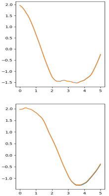
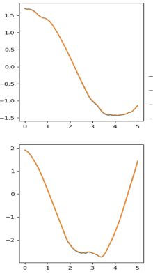
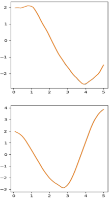
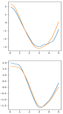
Figure 1. Sample neural SVE and DeepONet paths from the training and the test set for the disturbed pendulum equation and $n=100$. Blue (barely visible) are the original paths and orange the learned approximations.

3.2. Generalized Ornstein–Uhlenbeck process

The Ornstein–Uhlenbeck process, introduced in [UO30], is a commonly used stochastic process with applications finance, physics or biology, see e.g. [Vas12, TE99, Mar94]. We consider the generalized Ornstein–Uhlenbeck process that is given by the stochastic differential equation

$$\,\mathrm{d}X_{t}=\theta(\mu(t,X_{t})-X_{t})\,\mathrm{d}t+\sigma(t,X_{t})\,\mathrm{d}B_{t},\quad t\in[0,T],$$

which, using Itô’s formula, can be equivalently rewritten as the SVE

$$X_{t}=X_{0}e^{-\theta t}+\theta\int_{0}^{t}e^{-\theta(t-s)}\mu(s,X_{s})\,\mathrm{d}s+\int_{0}^{t}e^{-\theta(t-s)}\sigma(s,X_{s})\,\mathrm{d}B_{s},\quad t\in[0,T].$$

As prototyping example, we consider the one-dimensional equation

(3.2) $$X_{t}=\xi e^{-t}+\int_{0}^{t}e^{-(t-s)}X_{s}\,\mathrm{d}s+\int_{0}^{t}e^{-(t-s)}\sqrt{|X_{s}|}\,\mathrm{d}B_{s},\qquad t\in[0,T],$$

with the target to learn its dynamics by neural SVEs and DeepONet. The results are presented in Table 2.

Neural SVE	Train set	Test set
$n=100$	$0.015$	$0.038$
$n=500$	$0.014$	$0.036$
$n=2000$	$0.014$	$0.02$

DeepONet	Train set	Test set
$n=100$	$0.025$	$0.23$
$n=500$	$0.018$	$0.15$
$n=2000$	$0.028$	$0.12$

Table 2. Relative $L^{2}$-losses after training for the one-dimensional Ornstein–Uhlenbeck equation (3.2).

Example paths of the training and the testing sets together with their learned approximations are shown in Figure 2.

Neural SVE: Training set	Neural SVE: Test set	DeepONet: Training set	DeepONet: Test set

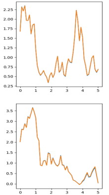
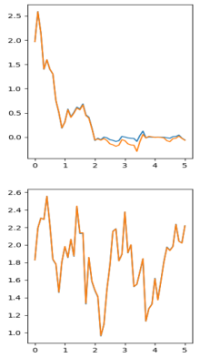
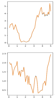
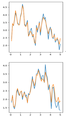
Figure 2. Sample neural SVE and DeepONet paths from the training and the test set for the one-dimensional Ornstein–Uhlenbeck equation and $n=500$. Blue (barely visible) are the original paths and orange the learned approximations.

Moreover, neural SVEs are able to learn multi-dimensional SVEs. As an example, we consider the two-dimensional equation

(3.3) $$\begin{pmatrix}X^{1}_{t}\\ X_{t}^{2}\end{pmatrix}=\begin{pmatrix}2\\ 2\end{pmatrix}e^{-t}+\int_{0}^{t}e^{-(t-s)}\begin{pmatrix}X^{1}_{s}\\ X_{s}^{2}\end{pmatrix}\,\mathrm{d}s+\int_{0}^{t}e^{-(t-s)}\begin{pmatrix}\sqrt{|X^{1}_{s}|},0\\ 0,\sqrt{|X_{s}^{2}|}\end{pmatrix}\,\mathrm{d}B_{s},\qquad t\in[0,T],$$

where $B$ is a $2$-dimensional Brownian motion, and try to learn its dynamics by neural SVEs. The results are presented in Table 3.

Neural SVE	Train set	Test set
$n=100$	$0.038$	$0.095$
$n=500$	$0.04$	$0.085$
$n=2000$	$0.038$	$0.04$

Table 3. Relative $L^{2}$-losses after training for the two-dimensional Ornstein–Uhlenbeck equation (3.3).

Example paths of the training and the testing sets together with their learned approximations are shown in Figure 3.

Neural SVE: Training set	Neural SVE: Test set

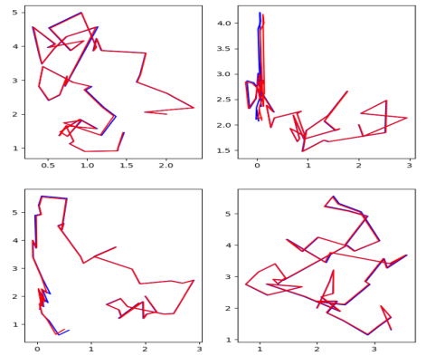
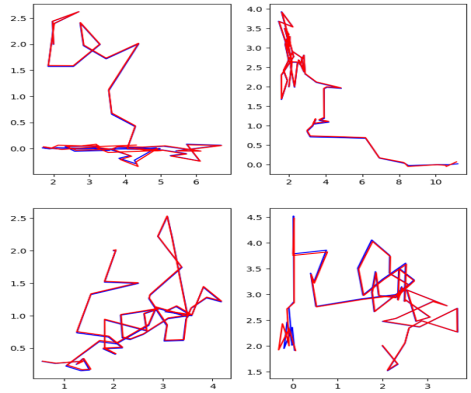
Figure 3. Sample neural SVE paths from the training and the test set for the two-dimensional Ornstein–Uhlenbeck equation and $n=2000$. Blue (barely visible) are the original paths and red the learned approximations.

3.3. Rough Heston equation

The rough Heston model is one of the most prominent representatives of rough volatility models in mathematical finance, see e.g. [EER19, AJEE19], where the volatility process is modeled by SVEs with the singular kernels $(t-s)^{-\alpha}$ for some $\alpha\in(0,1/2)$, that is

$$V_{t}=V_{0}+\frac{1}{\Gamma(\alpha)}\int_{0}^{t}(t-s)^{-\alpha}\lambda(\theta-V_{s})\,\mathrm{d}s+\frac{\lambda\nu}{\Gamma(\alpha)}\int_{0}^{t}(t-s)^{-\alpha}\sqrt{|V_{s}|}\,\mathrm{d}B_{s},\quad t\in[0,T],$$

where $\Gamma(x)=\int_{0}^{\infty}t^{x-1}e^{-t}\,\mathrm{d}t$ denotes the real valued Gamma function, and $\lambda,\theta,\nu\in\mathbb{R}$. As specific example, we consider the one-dimensional equation

(3.4) $$V_{t}=\xi+\frac{1}{\Gamma(0.4)}\int_{0}^{t}(t-s)^{-0.4}(2-V_{s})\,\mathrm{d}s+\frac{1}{\Gamma(0.4)}\int_{0}^{t}(t-s)^{-0.4}\sqrt{|V_{s}|}\,\mathrm{d}B_{s},\qquad t\in[0,T],$$

with the target to learn its dynamics by neural SVEs and DeepONet. The results are presented in Table 4. Neural SVEs outperform DeepONet here by far.

Neural SVE	Train set	Test set
$n=100$	$0.003$	$0.003$
$n=500$	$0.0025$	$0.0028$
$n=2000$	$0.0015$	$0.0017$

DeepONet	Train set	Test set
$n=100$	$0.035$	$0.13$
$n=500$	$0.004$	$0.037$
$n=2000$	$0.003$	$0.014$

Table 4. Relative $L^{2}$-losses after training for the rough Heston equation (3.4).

Example paths of the training and the testing sets together with their learned approximations are shown in Figure 4.

Neural SVE: Training set	Neural SVE: Test set	DeepONet: Training set	DeepONet: Test set

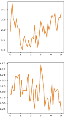
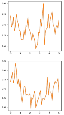
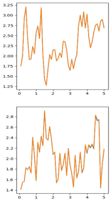
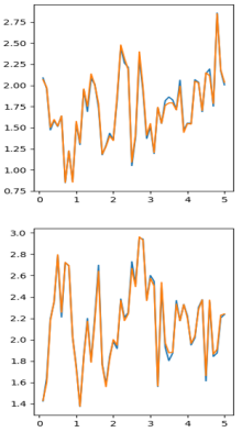
Figure 4. Sample neural SVE and DeepONet paths from the training and the test set for the rough Heston equation and $n=2000$. Blue (barely visible) are the original paths and orange the learned approximations.

3.4. Comparison to neural SDEs

Introduced in [Kid22], a neural stochastic differential equation (neural SDE) is defined by

$$Z_{0} =L_{\theta}(\xi),$$

$$Z_{t} =Z_{0}\,g_{\theta}(t)+\int_{0}^{t}\mu_{\theta}(s,Z_{s})\,\mathrm{d}s+\int_{0}^{t}\sigma_{\theta}(s,Z_{s})\,\mathrm{d}B_{s},$$

$$X_{t} =\Pi_{\theta}(Z_{t}),\quad t\in[0,T],$$

where all objects are defined as in the neural SVE (2.1). Since a neural SDE does not possess the kernel functions $K_{\mu,\theta}$ and $K_{\sigma,\theta}$ compared to the neural SVE (2.1), it is not able to fully capture the dynamics induced by SVEs.

Note that due to the need of discretizing the time interval when it comes to computations, some of the properties introduced by the kernels are attenuated. However, the memory structure of an SVE is a property which can be learned by a neural SVE but, in general, not by a neural SDE since SDEs posses the Markov property. Therefore, to see the potential capabilities of neural SVEs compared to neural SDEs, it is best to look at examples where the dependency on the whole path plays a crucial role. To construct such an example, we consider the kernels

$$K_{\mu}(s,t):=K_{\sigma}(s,t):=K(t-s)=\begin{cases}1,\quad&\text{if }(t-s)\leq T/4,\\ -1,\quad&\text{if }(t-s)>T/4,\end{cases}$$

and aim to learn the dynamics to the one-dimensional SVE

(3.5) $$X_{t}=\xi+\int_{0}^{t}K(t-s)(2-X_{s})\,\mathrm{d}s+\int_{0}^{t}K(t-s)\sqrt{|X_{s}|}\,\mathrm{d}B_{s},\qquad t\in[0,T],$$

where $\xi\sim\mathcal{N}(5,0.5)$ and $T=5$. The process $(X_{t})_{t\in[0,5]}$ is expected to decrease in the first quarter of the interval $[0,5]$ where $K(t-s)=1$ holds due to the mean-reverting effect of the drift coefficient $\mu(s,x)=2-x$, then something unpredictable will happen and finally in the last part of the interval $t\in[0,5]$ where the kernels attain $-1$ for a large proportion of $s\in[0,t]$, the process might become big due to the turning sign in the drift. Hence, it is expected that the path dependency will have a substantial impact.

We learn the dynamics of equation (3.5) simulated on an equally-sized grid with grid size $\Delta t=0.1$ by a neural SDE and by a neural SVE for a dataset of size $n=500$ and compare the results in Table 5. It can be observed that the neural SDE fails to learn the dynamics of (3.5) properly while the neural SVE performs well.

Neural SVE	Train set	Test set
$n=500$	$0.008$	$0.009$

Neural SDE	Train set	Test set
$n=500$	$0.19$	$0.21$

Table 5. Relative $L^{2}$-losses after training for the SVE (3.5).

Example paths of the training and the testing sets together with their learned approximations are shown in Figure 5.

Neural SVE: Training set	Neural SVE: Test set	Neural SDE: Training set	Neural SDE: Test set

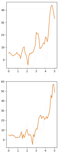
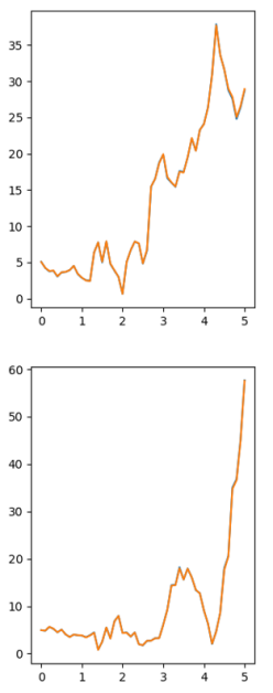
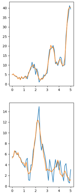
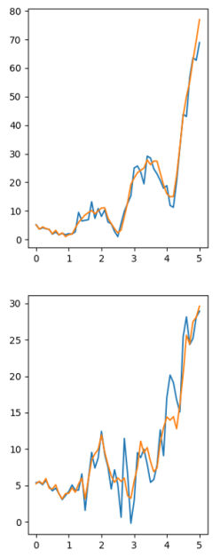
Figure 5. Sample neural SVE and neural SDE paths from the training and the test set for the SVE (3.5) and $n=500$. Blue are the original paths and orange the learned approximations.

References

- [AJEE19] Eduardo Abi Jaber and Omar El Euch, Multifactor approximation of rough volatility models, SIAM J. Financial Math. 10 (2019), no. 2, 309–349.
- [BNS08] Ole E. Barndorff-Nielsen and Jürgen Schmiegel, Time change, volatility, and turbulence, Mathematical control theory and finance, Springer, Berlin, 2008, pp. 29–53.
- [CBDJ19] Ricky T. Q. Chen, Jens Behrmann, David K. Duvenaud, and Joern-Henrik Jacobsen, Residual flows for invertible generative modeling, Advances in Neural Information Processing Systems (H. Wallach, H. Larochelle, A. Beygelzimer, F. d'Alché-Buc, E. Fox, and R. Garnett, eds.), vol. 32, Curran Associates, Inc., 2019.
- [CD01] L. Coutin and L. Decreusefond, Stochastic Volterra equations with singular kernels, Stochastic analysis and mathematical physics, Progr. Probab., vol. 50, Birkhäuser Boston, Boston, MA, 2001, pp. 39–50.
- [CKT20] Christa Cuchiero, Wahid Khosrawi, and Josef Teichmann, A generative adversarial network approach to calibration of local stochastic volatility models, Risks 8 (2020), no. 4.
- [CLP95] W. George Cochran, Jung-Soon Lee, and Jürgen Potthoff, Stochastic Volterra equations with singular kernels, Stochastic Process. Appl. 56 (1995), no. 2, 337–349.
- [CRBD18] Ricky T. Q. Chen, Yulia Rubanova, Jesse Bettencourt, and David Duvenaud, Neural ordinary differential equations, Proceedings of the 32nd International Conference on Neural Information Processing Systems, 2018, pp. 6572–6583.
- [CRW22] Samuel N. Cohen, Christoph Reisinger, and Sheng Wang, Hedging option books using neural-SDE market models, Appl. Math. Finance 29 (2022), no. 5, 366–401.
- [Cyb89] G. Cybenko, Approximation by superpositions of a sigmoidal function, Math. Control Signals Systems 2 (1989), no. 4, 303–314.
- [E17] Weinan E, A proposal on machine learning via dynamical systems, Commun. Math. Stat. 5 (2017), no. 1, 1–11.
- [EER19] Omar El Euch and Mathieu Rosenbaum, The characteristic function of rough Heston models, Math. Finance 29 (2019), no. 1, 3–38.
- [GSVS+22] Patrick Gierjatowicz, Marc Sabate-Vidales, David Siska, Lukasz Szpruch, and Zan Zuric, Robust pricing and hedging via neural stochastic differential equations, Journal of Computational Finance 26 (2022), no. 3, 1–32.
- [Hor91] Kurt Hornik, Approximation capabilities of multilayer feedforward networks, Neural Networks 4 (1991), no. 2, 251–257.
- [IHLS24] Zacharia Issa, Blanka Horvath, Maud Lemercier, and Cristopher Salvi, Non-adversarial training of Neural SDEs with signature kernel scores, Advances in Neural Information Processing Systems 36 (2024).
- [KB14] Diederik P. Kingma and Jimmy Ba, Adam: A method for stochastic optimization, ArXiv Preprint arXiv:1412.6980 (2014).
- [KFLL21] Patrick Kidger, James Foster, Xuechen Li, and Terry Lyons, Efficient and Accurate Gradients for Neural SDEs, arXiv preprint arXiv:2105.13493 (2021).
- [Kid22] Patrick Kidger, On Neural Differential Equations, ArXiv Preprint arXiv:2202.02435 (2022).
- [KMFL20] Patrick Kidger, James Morrill, James Foster, and Terry Lyons, Neural controlled differential equations for irregular time series, Advances in Neural Information Processing Systems 33 (2020), 6696–6707.
- [Kre99] Erwin Kreyszig, Advanced engineering mathematics, eighth ed., John Wiley & Sons, Inc., New York, 1999.
- [KS91] Ioannis Karatzas and Steven E. Shreve, Brownian motion and stochastic calculus, second ed., Graduate Texts in Mathematics, vol. 113, Springer-Verlag, New York, 1991.
- [LJP+21] Lu Lu, Pengzhan Jin, Guofei Pang, Zhongqiang Zhang, and George Karniadakis, Learning nonlinear operators via deeponet based on the universal approximation theorem of operators, Nature Machine Intelligence 3 (2021), 218–229.
- [LWCD20] Xuechen Li, Ting-Kam Leonard Wong, Ricky TQ Chen, and David Duvenaud, Scalable gradients for stochastic differential equations, International Conference on Artificial Intelligence and Statistics, PMLR, 2020, pp. 3870–3882.
- [LXS+19] Xuanqing Liu, Tesi Xiao, Si Si, Qin Cao, Sanjiv Kumar, and Cho-Jui Hsieh, Neural SDE: Stabilizing Neural ODE Networks with Stochastic Noise, ArXiv preprint arXiv:1906.02355 (2019).
- [Mar94] Emilia P. Martins, Estimating the rate of phenotypic evolution from comparative data, The American Naturalist 144 (1994), no. 2, 193–209.
- [MSKF21] James Morrill, Cristopher Salvi, Patrick Kidger, and James Foster, Neural rough differential equations for long time series, International Conference on Machine Learning, PMLR, 2021, pp. 7829–7838.
- [Øks03] Bernt Øksendal, Stochastic differential equations, sixth ed., Universitext, Springer-Verlag, Berlin, 2003, An introduction with applications.
- [PP90] Étienne Pardoux and Philip Protter, Stochastic Volterra equations with anticipating coefficients, Ann. Probab. 18 (1990), no. 4, 1635–1655.
- [PS23] David J. Prömel and David Scheffels, Stochastic Volterra equations with Hölder diffusion coefficients, Stochastic Process. Appl. 161 (2023), 291–315.
- [RBS10] Patricia Reynaud-Bouret and Sophie Schbath, Adaptive estimation for Hawkes processes; application to genome analysis, Ann. Statist. 38 (2010), no. 5, 2781–2822.
- [RZL17] Prajit Ramachandran, Barret Zoph, and Quoc V. Le, Searching for Activation Functions, ArXiv Preprint arXiv:1710.05941 (2017).
- [SLG22] Cristopher Salvi, Maud Lemercier, and Andris Gerasimovics, Neural Stochastic PDEs: Resolution-Invariant Learning of Continuous Spatiotemporal Dynamics, 36th Conference on Neural Information Processing Systems (NeurIPS), 2022.
- [TE99] Erkan Tuzel and Ayse Erzan, Dissipative Dynamics and the Statistics of Energy States of a Hookean Model for Protein Folding, ArXiv Preprint cond-mat/9909350 (1999).
- [UO30] G. E. Uhlenbeck and L. S. Ornstein, On the Theory of the Brownian Motion, Phys. Rev. 36 (1930), 823–841.
- [Vas12] Oldrich Vasicek, An equilibrium characterization of the term structure [reprint of J. Financ. Econ. 5 (1977), no. 2, 177–188], Financial risk measurement and management, Internat. Lib. Crit. Writ. Econ., vol. 267, Edward Elgar, Cheltenham, 2012, pp. 724–735.
- [Wan08] Zhidong Wang, Existence and uniqueness of solutions to stochastic Volterra equations with singular kernels and non-Lipschitz coefficients, Statist. Probab. Lett. 78 (2008), no. 9, 1062–1071.
- [YYK15] Neha Yadav, Anupam Yadav, and Manoj Kumar, An introduction to neural network methods for differential equations, SpringerBriefs in Applied Sciences and Technology, Springer, Dordrecht, 2015.
- [Zha08] Xicheng Zhang, Euler schemes and large deviations for stochastic Volterra equations with singular kernels, J. Differential Equations 244 (2008), no. 9, 2226–2250.