Contraction of unitary operators, quantum graphs and quantum channels

Abstract

Given a unitary operator in a finite dimensional complex Hilbert space, its unitary contraction to a subspace is defined. The application to quantum graphs is discussed. It is shown how the contraction allows to generate the scattering matrices of new quantum graphs from assembling of simpler graphs. The contraction of quantum channels is also defined. The implementation of the quantum gates corresponding to the contracted unitary operator is investigated, although no explicit construction is presented. The situation is different for the contraction of quantum channels for which explicit implementations are given.

I Introduction

In this work we introduce the concept of contraction of a unitary operator to produce another unitary operator which acts in a subspace. The concept originates in the context of quantum graphs. Quantum graphs describe a quantum particle, which may have spin, or be relativistic, moving on a net of lines connected at nodes, forming a graph. The graph may be compact, the Hamiltonian having only a discrete spectrum, or non compact, so that the particle may go towards (or come from) infinity along several leads. In the latter case a scattering matrix may be defined under suitable assumptions ensuring that the particle moves freely in the asymptotic region. Since the kinematics is trivial in the asymptotic region, when two graphs are joined to form a larger graph, the scattering matrix of the latter is determined by the scattering matrices of the components (plus information on the junctions, namely, their lengths). The resulting formula is an instance of contraction of unitary operators. The adopted name of “contraction” comes from this context and also because it loosely recalls (a nonlinear version of) the contraction of a tensor to produce a tensor of lower rank.

The contraction of finite-dimensional unitary operators is defined and analyzed here from the mathematical point of view. It is shown that it exists with no restrictions on the unitary operators or the subspaces. The contraction may be introduced through a set of equations or as the sum of a series. Both approaches are discussed in Sec. II and several properties of the contraction are uncovered, providing the corresponding mathematical proofs. Sec. III introduces quantum graphs. The relation of the contraction of graphs, or rather their scattering matrices, with the contraction of unitary operators is established. In the first part of Sec. IV we investigate the contraction of general, i.e., non-unitary, operators within the two approaches (equations and series). Not surprisingly, at variance with the unitary case, the operators should fulfill some specific requirements for the existence of the contraction. In the second part of Sec. IV the concept of contraction is extended to quantum channels. Necessary and sufficient conditions on the quantum channels are established for the contraction to exist. Finally, in Sec. V we consider the possible implementation of the unitary contraction in the context of quantum computation. Certainly every finite unitary quantum gate can be constructed using circuits but in general this requires a detailed knowledge of the corresponding unitary operator. What is studied here is whether a circuit implementing the contraction can be produced given the unitary operator to be contracted as a black box. The problem is related to the introduction of loops is a quantum circuit. Our analysis does not find a positive answer, but it does for the related problem of the contraction of quantum channels.

II Contraction of a unitary operator to a subspace

II.1 Definitions and main theorem

In this work all abstract vector spaces considered are complex and finite dimensional, unless otherwise specified. In the case of Hilbert spaces $\oplus$ denotes the direct sum of orthogonal subspaces, $\subseteq$ denotes subspace, and $\ominus$ denotes orthogonal complement.

Lemma 1  Let ${\mathcal{W}}\subseteq{\mathcal{A}}\oplus{\mathcal{B}}$ be a relation between Hilbert spaces. Then

$${\mathcal{W}}=W{\mathcal{A}}\oplus{\mathcal{W}}\cap{\mathcal{B}},$$ (1)

where $W$ is the orthogonal projector operator onto the subspace ${\mathcal{W}}$.

Proof  Let $\varphi\in{\mathcal{W}}$. Then $\varphi\in{\mathcal{B}}\iff\varphi\perp{\mathcal{A}}\iff\varphi\perp W{\mathcal{A}}$. This implies ${\mathcal{W}}\cap{\mathcal{B}}={\mathcal{W}}\ominus W{\mathcal{A}}$. $\square$

Let $U:{\mathcal{H}}\to{\mathcal{F}}$ and $\varOmega:{\mathcal{F}}_{1}\to{\mathcal{H}}_{1}$ be unitary operators between Hilbert spaces with ${\mathcal{F}}_{1}\subseteq{\mathcal{F}}$ and ${\mathcal{H}}_{1}\subseteq{\mathcal{H}}$. Let ${\mathcal{H}}_{0}:={\mathcal{H}}\ominus{\mathcal{H}}_{1}$ and ${\mathcal{F}}_{0}:={\mathcal{F}}\ominus{\mathcal{F}}_{1}$. Then the equations

$$\phi_{0}+\phi_{1}=U(\psi_{0}+\psi_{1}),\qquad\psi_{1}=\varOmega\phi_{1},$$ (2)

with unknowns $\psi_{1}\in{\mathcal{H}}_{1}$, $\phi_{0}\in{\mathcal{F}}_{0}$ and $\phi_{1}\in{\mathcal{F}}_{1}$, have a solution for any given $\psi_{0}\in{\mathcal{H}}_{0}$. Furthermore the solution is unique for $\phi_{0}$ and $\|\phi_{0}\|=\|\psi_{0}\|$.

Proof  Let $H_{j}$ and $F_{j}$, for $j\in\{0,1\}$, denote the orthogonal projector operators onto ${\mathcal{H}}_{j}$ and ${\mathcal{F}}_{j}$, respectively. Then, upon elimination of $\psi_{1}$ in favor of $\phi_{1}$, the conditions can be expressed as

$$\begin{split}\phi_{0}&=F_{0}U\psi_{0}+F_{0}U\varOmega\phi_{1},\\ \phi_{1}&=F_{1}U\psi_{0}+F_{1}U\varOmega\phi_{1},\end{split}$$ (3)

and the second equation is equivalent to

$$F_{1}U\psi_{0}=(I-F_{1}U\varOmega)\phi_{1}.$$ (4)

This equation can be solved for $\phi_{1}$, for arbitrary $\psi_{0}\in{\mathcal{H}}_{0}$, if and only if $F_{1}U{\mathcal{H}}_{0}\subseteq(I-F_{1}U\varOmega){\mathcal{F}}_{1}$.

Let

$${\mathcal{V}}_{1}:=\{\varphi_{1}\in{\mathcal{F}}_{1}~{}|~{}U\varOmega\varphi_{1}=\varphi_{1}\}.$$ (5)

Let us show that ${\mathcal{V}}_{1}$ is the kernel of the operator $(I-F_{1}U\varOmega):{\mathcal{F}}_{1}\to{\mathcal{F}}_{1}$. Clearly, $\varphi_{1}\in{\mathcal{V}}_{1}\implies(I-F_{1}U\varOmega)\varphi_{1}=0$. And vice versa, $F_{1}U\varOmega\varphi_{1}=\varphi_{1}$ implies that $U\varOmega\varphi_{1}=\varphi_{1}+\varphi_{0}$ with $\varphi_{0}\in{\mathcal{F}}_{0}$. However necessarily $\varphi_{0}=0$ because $U\varOmega$ is unitary, hence $\varphi_{1}\in{\mathcal{V}}_{1}$. That ${\mathcal{V}}_{1}$ is the kernel implies that $\dim{\mathcal{V}}_{1}+\dim(I-F_{1}U\varOmega){\mathcal{F}}_{1}=\dim{\mathcal{F}}_{1}$. As a consequence

$${\mathcal{F}}_{1}={\mathcal{V}}_{1}\oplus(I-F_{1}U\varOmega){\mathcal{F}}_{1}.$$ (6)

To show this, first note that ${\mathcal{V}}_{1}\perp(I-F_{1}U\varOmega){\mathcal{F}}_{1}$, hence $(I-F_{1}U\varOmega){\mathcal{F}}_{1}\subseteq{\mathcal{F}}_{1}\ominus{\mathcal{V}}_{1}$. But the spaces $(I-F_{1}U\varOmega){\mathcal{F}}_{1}$ and ${\mathcal{F}}_{1}\ominus{\mathcal{V}}_{1}$ have the same dimension so they must coincide.

Next we make use of the relation

$$F_{1}U{\mathcal{H}}_{0}\oplus{\mathcal{F}}_{1}\cap U{\mathcal{H}}_{1}={\mathcal{F}}_{1}\,,$$ (7)

which is a consequence of Lemma II.1 and ${\mathcal{F}}=U{\mathcal{H}}_{0}\oplus U{\mathcal{H}}_{1}$. Then, using ${\mathcal{H}}_{1}=\varOmega{\mathcal{F}}_{1}$,

$$\begin{split}&{\mathcal{V}}_{1}\subseteq{\mathcal{F}}_{1}\cap U\varOmega{\mathcal{F}}_{1}={\mathcal{F}}_{1}\cap U{\mathcal{H}}_{1}={\mathcal{F}}_{1}\ominus F_{1}U{\mathcal{H}}_{0}\\ &\implies~{}F_{1}U{\mathcal{H}}_{0}\subseteq{\mathcal{F}}_{1}\ominus{\mathcal{V}}_{1}=(I-F_{1}U\varOmega){\mathcal{F}}_{1}.\end{split}$$ (8)

This guarantees that (4) has solutions for arbitrary $\psi_{0}$.

The solutions to (4) have the form $\phi_{1}=\phi_{1}^{\prime}+\varphi_{1}$, where $\varphi_{1}$ is an arbitrary vector of ${\mathcal{V}}_{1}$ while $\phi_{1}^{\prime}\in{\mathcal{F}}_{1}\ominus{\mathcal{V}}_{1}$ is unique. In the first eq. (3) $F_{0}U\varOmega\varphi_{1}=F_{0}\varphi_{1}=0$, therefore

$$\phi_{0}=F_{0}U\psi_{0}+F_{0}U\varOmega\phi_{1}^{\prime}$$ (9)

uniquely determines $\phi_{0}$. This defines a linear map $\psi_{0}\to\phi_{0}$. $U$ is unitary hence $\|\psi_{0}\|^{2}+\|\psi_{1}\|^{2}=\|\phi_{0}\|^{2}+\|\phi_{1}\|^{2}$, and $\varOmega$ is also unitary, then $\|\psi_{1}\|=\|\phi_{1}\|$. This implies $\|\psi_{0}\|=\|\phi_{0}\|$. $\square$

Definition 1  (Contraction of a unitary map with a unitary suboperator)  The map $\psi_{0}\to\phi_{0}$ obtained in Theorem LABEL:th:1 will be denoted $\varOmega\cdot U$. The unitary operator $\varOmega\cdot U:{\mathcal{H}}_{0}\to{\mathcal{F}}_{0}$ is the contraction of $U:{\mathcal{H}}\to{\mathcal{F}}$ to ${\mathcal{H}}_{0}\to{\mathcal{F}}_{0}$ with connection $\varOmega:{\mathcal{F}}_{1}\to{\mathcal{H}}_{1}$, or simply, the contraction of $U$ to ${\mathcal{H}}_{0}$. The subspaces ${\mathcal{H}}_{1}$ and ${\mathcal{F}}_{1}$ have been contracted. $\diamondsuit$

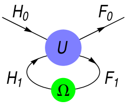
Figure 1: Schematics of the contraction.

Fig. 1 shows a cartoon of the unitary contraction setting.

Particular case 1  A particular case corresponds to ${\mathcal{H}}={\mathcal{F}}$, with ${\mathcal{H}}_{0}={\mathcal{F}}_{0}$ and ${\mathcal{H}}_{1}={\mathcal{F}}_{1}$, and $\varOmega$ is the identity operator in ${\mathcal{H}}_{1}$. This can be denoted $I_{{\mathcal{H}}_{1}}\cdot U$ o even ${\mathcal{H}}_{1}\cdot U$, the contraction of $U$ to the subspace ${\mathcal{H}}\ominus{\mathcal{H}}_{1}$. $\diamondsuit$

The component of $\phi_{1}$ along the subspace ${\mathcal{V}}_{1}$ is left undetermined and it can be set to $0$ as it does no have a contribution to the final value of $\phi_{0}$. Such component does not originate from the initial $\psi_{0}$, and the pair of subspaces ${\mathcal{V}}_{1}\subseteq{\mathcal{F}}_{1}$ and its image $\varOmega{\mathcal{V}}_{1}\subseteq{\mathcal{H}}_{1}$ completely decouple from the rest in the map $\varOmega\cdot U$.

Lemma 2  Let ${\mathcal{V}}\subseteq{\mathcal{F}}_{1}\cap U{\mathcal{H}}_{1}$ be the largest subspace which is invariant under $U\varOmega:{\mathcal{F}}_{1}\to U{\mathcal{H}}_{1}$, namely the sum of all $U\varOmega$-invariant subspaces. In particular ${\mathcal{V}}_{1}\subseteq{\mathcal{V}}$. Then the map $\varOmega\cdot U:{\mathcal{H}}_{0}\to{\mathcal{F}}_{0}$ is unchanged if the subspaces ${\mathcal{V}}$ and $\varOmega{\mathcal{V}}$ are stripped from ${\mathcal{F}}_{1}$ and ${\mathcal{H}}_{1}$ respectively (and so from ${\mathcal{F}}$ and ${\mathcal{H}}$). Also unchanged are the operators

$$(U\varOmega F_{1})^{n}UH_{0}\qquad n\geq 0.$$ (10)

Proof  $\varOmega\cdot U$ will be unchanged if the equations (2) still have a solution adding the new condition $\varphi_{V}=0$, where $\varphi_{V}:=F_{V}\phi_{1}$ and $F_{V}$ is the orthogonal projector onto ${\mathcal{V}}$.

Let ${\mathcal{F}}_{1}^{\prime}:={\mathcal{F}}_{1}\ominus{\mathcal{V}}$. Then the vector $\phi_{1}$ can be split as $\phi_{1}=\phi_{1}^{\prime}+\varphi_{V}$, where $\phi_{1}^{\prime}\in{\mathcal{F}}_{1}^{\prime}$ and $\varphi_{V}\in{\mathcal{V}}$. The projection of the equation $\phi_{0}+\phi_{1}=U(\psi_{0}+\varOmega\phi_{1})$ onto ${\mathcal{V}}$ produces

$$\varphi_{V}=F_{V}U\psi_{0}+F_{V}U\varOmega\phi_{1}^{\prime}+F_{V}U\varOmega\varphi_{V}.$$ (11)

In the RHS $F_{V}U\psi_{0}=0$ because ${\mathcal{V}}\subseteq U{\mathcal{H}}_{1}\perp U{\mathcal{H}}_{0}$. Also $F_{V}U\varOmega\phi_{1}^{\prime}=0$ because ${\mathcal{V}}\perp{\mathcal{F}}_{1}^{\prime}$ hence ${\mathcal{V}}=U\varOmega{\mathcal{V}}\perp U\varOmega{\mathcal{F}}_{1}^{\prime}$. In addition $F_{V}U\varOmega\varphi_{V}=U\varOmega\varphi_{V}$ due to ${\mathcal{V}}=U\varOmega{\mathcal{V}}$. The projected equation becomes $\varphi_{V}=U\varOmega\varphi_{V}$, and this implies that $\varphi_{V}=\varphi_{1}\in{\mathcal{V}}_{1}$. As already noted $\varphi_{1}$ is not determined by the equations and can be chosen to be zero. Therefore the constraint $\varphi_{V}=0$ does not modify $\phi_{0}$ nor the map $\varOmega\cdot U$.

To prove that the operators in eq. (10) are unchanged, let $F_{1}^{\prime}$ be the projector onto ${\mathcal{F}}_{1}^{\prime}$. The following relations are verified,

$$F_{V}UH_{0}=F_{V}F_{1}^{\prime}=0,\qquad[F_{V},U\varOmega]=0,\qquad F_{1}=F_{1}^{\prime}+F_{V}.$$ (12)

The statement is that $F_{1}^{\prime}$ can be used instead of $F_{1}$ in (10). This is trivial for $n=0$. For $n=1$

$$\begin{split}U\varOmega F_{1}UH_{0}&=U\varOmega(F_{1}^{\prime}+F_{V})UH_{0}\\ &=U\varOmega F_{1}^{\prime}UH_{0}.\end{split}$$ (13)

By induction, for $n\geq 2$,

$$\begin{split}(U\varOmega F_{1})^{n}UH_{0}&=U\varOmega(F_{1}^{\prime}+F_{V})(U\varOmega F_{1}^{\prime})^{n-1}UH_{0}\\ &=(U\varOmega F_{1}^{\prime})^{n}UH_{0}\end{split}$$ (14)

using $F_{V}U\varOmega F_{1}^{\prime}=U\varOmega F_{V}F_{1}^{\prime}=0$. $\square$

The lemma implies that in the construction of $\varOmega\cdot U$, the subspaces ${\mathcal{V}}$ and $\varOmega{\mathcal{V}}$ completely decouple from the rest.

Particular case 2  An extreme instance of decoupling takes place when ${\mathcal{F}}_{0}=U{\mathcal{H}}_{0}$ and ${\mathcal{F}}_{1}=U{\mathcal{H}}_{1}$. In this case ${\mathcal{V}}={\mathcal{F}}_{1}$ and the contraction $\varOmega\cdot U$ is just the restriction of $U$ to ${\mathcal{H}}_{0}\to{\mathcal{F}}_{0}$, regardless of the choice of $\varOmega$. $\diamondsuit$

Particular case 3  An opposite extreme situation is ${\mathcal{F}}_{1}=U{\mathcal{H}}_{0}$ and ${\mathcal{F}}_{0}=U{\mathcal{H}}_{1}$. In this case ${\mathcal{V}}=0$ and $\varOmega\cdot U=U\varOmega U$ as an operator from ${\mathcal{H}}_{0}$ to ${\mathcal{F}}_{0}$. $\diamondsuit$

The map $U\varOmega:{\mathcal{V}}\to{\mathcal{V}}$ is unitary, hence clearly, $\|F_{1}U\varOmega\|=1$ is a necessary (but not sufficient) condition for a non vanishing ${\mathcal{V}}$ or ${\mathcal{V}}_{1}$. The following lemma provides a necessary and sufficient condition.

Lemma 3  Let ${\mathcal{H}}$ be a Hilbert space, $U:{\mathcal{H}}\to{\mathcal{H}}$ a unitary operator and ${\mathcal{W}}$ a non-zero subspace of ${\mathcal{H}}$. Then ${\mathcal{W}}$ contains a non-zero $U$-invariant subspace if and only if $\|(WUW)^{d}\|=1$, where $W$ is the orthogonal projector onto ${\mathcal{W}}$ and $d=\dim{\mathcal{W}}$.

Proof  If there is a non-zero invariant subspace in ${\mathcal{W}}$, then there is an eigenvector of $U$ in ${\mathcal{W}}$ and this implies $\|(WUW)^{d}\|=1$. Let us now assume that $\|(WUW)^{d}\|=1$. In this case there is a unit vector $u_{0}\in{\mathcal{H}}$ such that $u_{d}:=W(UW)^{d}u_{0}$ is also a unit vector. Clearly $u_{0}\in{\mathcal{W}}$, otherwise $\|Wu_{0}\|<1$ and this would imply $\|u_{d}\|<1$. By the same token, all the vectors $u_{k}:=U^{k}u_{0}$ for $k=0,\ldots,d$ must fulfill $u_{k}\in{\mathcal{W}}$ to ensure $\|u_{d}\|=1$. Since no $d+1$ vectors can be linearly independent in ${\mathcal{W}}$ it follows that one of them, $u_{k_{0}}$, must be a linear combination of the previous ones, and in this case the vectors $u_{0},\ldots,u_{k_{0}-1}$ span a non-zero subspace which is invariant under $U$. $\square$

The same statement holds for any exponent $d^{\prime}\geq d$ instead of $d$.

Example 1  As a simple example, let

$$U=\begin{pmatrix}t&-\omega r^{*}\\ r&\omega t^{*}\end{pmatrix},\quad t,r,\omega\in\mathbb{C},\quad|t|^{2}+|r|^{2}=|\omega|=1\,.$$ (15)

$U$ is a generic unitary matrix in ${\mathcal{H}}={\mathcal{F}}=\mathbb{C}^{2}$. Furthermore ${\mathcal{H}}_{0}={\mathcal{F}}_{0}$ and ${\mathcal{H}}_{1}={\mathcal{F}}_{1}$ are spanned by the upper and lower components, respectively. The map $\varOmega$ is codified by a number $\varOmega\in\mathbb{C}$, $|\varOmega|=1$. The equations defining the contraction are

$$\begin{pmatrix}\phi_{0}\\ \phi_{1}\end{pmatrix}=\begin{pmatrix}t&-\omega r^{*}\\ r&\omega t^{*}\end{pmatrix}\begin{pmatrix}\psi_{0}\\ \psi_{1}\end{pmatrix},\qquad\psi_{1}=\varOmega\phi_{1}\,.$$ (16)

Three cases can be distinguished:

• $r\neq 0$. Then ${\mathcal{F}}_{1}\cap U{\mathcal{H}}_{1}=0$.

• $r=0$ and $t\neq\omega\varOmega$. Then ${\mathcal{V}}=U{\mathcal{H}}_{1}={\mathcal{F}}_{1}$ and ${\mathcal{V}}_{1}=0$.

  In any of these two cases $\phi_{1}$ is unique, and

  $$\phi_{1}=\frac{r}{1-\omega\varOmega t^{*}}\psi_{0},\qquad\phi_{0}=-\frac{1}{\omega\varOmega}\frac{t-\omega\varOmega}{(t-\omega\varOmega)^{*}}\psi_{0}.$$ (17)

  The map $\psi_{0}\to\phi_{0}$ depends only on the combination $\omega\varOmega$ and not on (the phase of) $r$. It is also noteworthy that $\|\phi_{1}\|$ is not bounded, for fixed $\|\psi_{0}\|$.

• $t=\omega\varOmega$. Then ${\mathcal{V}}_{1}={\mathcal{F}}_{1}$, $\phi_{1}$ is arbitrary, and $\phi_{0}=t\psi_{0}$.

In all cases the map $\psi_{0}\to\phi_{0}$ is manifestly unitary. The map $\varOmega\cdot U$ is not a continuous function of $U$ and $\varOmega$ at $t=\omega\varOmega$. The value of $\varOmega\cdot U$ at $t=\omega\varOmega$ coincides with the limit taken on the set $|t|=1$. On this set $r=0$ and $\phi_{1}$ vanishes (for $t\neq\omega\varOmega$). In the cases i) and iii) reciprocity applies (see Theorem LABEL:th:2 below). $\diamondsuit$

II.2 Some properties of the contraction

The following proposition shows that performing two contractions sequentially is equivalent to doing the contraction in a single step.

Proposition 1  (Sequential contractions)  Let ${\mathcal{H}}={\mathcal{H}}_{0}\oplus{\mathcal{H}}_{1}\oplus{\mathcal{H}}_{2}$ and ${\mathcal{F}}={\mathcal{F}}_{0}\oplus{\mathcal{F}}_{1}\oplus{\mathcal{F}}_{2}$ be Hilbert spaces, and let $U:{\mathcal{H}}\to{\mathcal{F}}$, $\varOmega_{1}:{\mathcal{F}}_{1}\to{\mathcal{H}}_{1}$ and $\varOmega_{2}:{\mathcal{F}}_{2}\to{\mathcal{H}}_{2}$ be unitary maps. Then

$$(\varOmega_{1}\oplus\varOmega_{2})\cdot U=\varOmega_{1}\cdot(\varOmega_{2}\cdot U)$$ (18)

Proof  Let us make use of the decompositions $\psi=\psi_{01}+\psi_{2}=\psi_{0}+\psi_{1}+\psi_{2}$, and $\phi=\phi_{01}+\phi_{2}=\phi_{0}+\phi_{1}+\phi_{2}$. The first contraction $\phi_{01}=\varOmega_{2}\cdot U\psi_{01}$ is determined by the equations

$$\phi=U\psi,\qquad\varOmega_{2}\phi_{2}=\psi_{2},$$ (19)

upon elimination of $\psi_{2}$ and $\phi_{2}$. Likewise, the second contraction is determined by the equations

$$\phi_{01}=\varOmega_{2}\cdot U\psi_{01},\qquad\varOmega_{1}\phi_{1}=\psi_{1},$$ (20)

upon elimination of $\psi_{1}$ and $\phi_{1}$. Hence the final map $\psi_{0}\to\phi_{0}$ is determined by the conditions

$$\phi=U\psi,\qquad\varOmega_{1}\phi_{1}=\psi_{1},\qquad\varOmega_{2}\phi_{2}=\psi_{2}.$$ (21)

This is the same set of equations that would be produced by eliminating ${\mathcal{H}}_{1}\oplus{\mathcal{H}}_{2}$ with the connection $\varOmega_{1}\oplus\varOmega_{2}$. $\square$

Another similar proposition is as follows:

Proposition 2  Let ${\mathcal{H}}={\mathcal{H}}_{0}\oplus{\mathcal{H}}_{1}$ and ${\mathcal{F}}={\mathcal{F}}_{0}\oplus{\mathcal{F}}_{1}$ be Hilbert spaces, and let $U:{\mathcal{H}}\to{\mathcal{F}}$ and $\varOmega:{\mathcal{F}}_{1}\to{\mathcal{H}}_{1}$ be unitary maps. Then

$$\varOmega^{-1}\cdot U^{-1}=(\varOmega\cdot U)^{-1}$$ (22)

Proof  Let us make use of the decompositions $\psi=\psi_{0}+\psi_{1}$, and $\phi=\phi_{0}+\phi_{1}$. The contraction $\phi_{0}=\varOmega\cdot U\psi_{0}$ is determined by the equations

$$\phi=U\psi,\qquad\varOmega\phi_{1}=\psi_{1},$$ (23)

upon elimination of $\psi_{1}$ and $\phi_{1}$. These conditions are equivalent to

$$\psi=U^{-1}\phi,\qquad\varOmega^{-1}\psi_{1}=\phi_{1},$$ (24)

which define the map $\psi_{0}=\varOmega^{-1}\cdot U^{-1}\phi_{0}$. $\square$

Some properties under chiral transformations are also easily established:

Proposition 3  Let $Q_{0}$, $Q_{1}$, $R_{0}$ and $R_{1}$ be unitary maps acting in ${\mathcal{H}}_{0}$, ${\mathcal{H}}_{1}$, ${\mathcal{F}}_{0}$ and ${\mathcal{F}}_{1}$, respectively, and they are naturally extended as the identity in the complementary spaces. Then

$$\varOmega\cdot(R_{0}R_{1}UQ_{0}Q_{1})=R_{0}(Q_{1}\varOmega R_{1}\cdot U)Q_{0}.$$ (25)

Proof   The map $\varOmega\cdot(R_{0}R_{1}UQ_{0}Q_{1})$ is defined by the following equations

$$\phi_{0}+\phi_{1}=R_{0}R_{1}UQ_{0}Q_{1}(\psi_{0}+\psi_{1}),\qquad\psi_{1}=\varOmega\phi_{1}.$$ (26)

This implies

$$R_{0}^{-1}\phi_{0}+R_{1}^{-1}\phi_{1}=U(Q_{0}\psi_{0}+Q_{1}\varOmega\phi_{1}).$$ (27)

Let us define

$$\phi_{0}^{\prime}=R_{0}^{-1}\phi_{0},\qquad\phi_{1}^{\prime}=R_{1}^{-1}\phi_{1},\qquad\psi_{0}^{\prime}=Q_{0}\psi_{0}.$$ (28)

The equation is then equivalent to

$$\phi_{0}^{\prime}+\phi_{1}^{\prime}=U(\psi_{0}^{\prime}+Q_{1}\varOmega R_{1}\phi_{1}^{\prime}).$$ (29)

Therefore $(Q_{1}\varOmega R_{1}\cdot U)\psi_{0}^{\prime}=\phi_{0}^{\prime}$, and $\eqref{eq:1.22}$ follows. $\square$

As well as properties under tensor product:

Proposition 4  Let $U:{\mathcal{H}}_{0}\oplus{\mathcal{H}}_{1}\to{\mathcal{F}}_{0}\oplus{\mathcal{F}}_{1}$, $\varOmega:{\mathcal{F}}_{1}\to{\mathcal{H}}_{1}$, and $V:{\mathcal{H}}^{\prime}\to{\mathcal{F}}^{\prime}$, be unitary operators. Then

$$(\varOmega\otimes V^{-1})\cdot(U\otimes V)=(\varOmega\cdot U)\otimes V$$ (30)

Proof  The map on the LHS is defined by the equations

$$\Phi_{0}+\Phi_{1}=U\otimes V(\Psi_{0}+\Psi_{1}),\qquad\varOmega\otimes V^{-1}\Phi_{1}=\Psi_{1},$$ (31)

where $\Psi_{0}$, $\Psi_{1}$, $\Phi_{0}$ and $\Phi_{1}$ are vectors in ${\mathcal{H}}_{0}\otimes{\mathcal{H}}^{\prime}$, ${\mathcal{H}}_{1}\otimes{\mathcal{H}}^{\prime}$, ${\mathcal{F}}_{0}\otimes{\mathcal{F}}^{\prime}$ and ${\mathcal{F}}_{1}\otimes{\mathcal{F}}^{\prime}$, respectively. The map is $\Psi_{0}\to\Phi_{0}$ and it is sufficient to consider the case of a separable $\Psi_{0}$,

$$\Psi_{0}=\psi_{0}\otimes\psi^{\prime},\qquad\psi_{0}\in{\mathcal{H}}_{0},\quad\psi^{\prime}\in{\mathcal{H}}^{\prime}.$$ (32)

Since $\Phi_{0}$ is uniquely defined by the equations, new constraints on $\Phi$ and $\Psi_{1}$ can be added if the prove to be compatible. So we add the equations

$$\begin{split}\Phi_{0}&=\phi_{0}\otimes\phi^{\prime},\quad\Phi_{1}=\phi_{1}\otimes\phi^{\prime},\quad\\ \Psi_{1}&=\psi_{1}\otimes\psi^{\prime},\quad\phi^{\prime}=V\psi^{\prime},\\ \phi_{0}&\in{\mathcal{F}}_{0},\quad\phi_{1}\in{\mathcal{F}}_{1},\quad\psi_{1}\in{\mathcal{H}}_{1},\quad\phi^{\prime}\in{\mathcal{F}}^{\prime}\,.\end{split}$$ (33)

Substitution in (31) yields

$$\begin{split}(\phi_{0}+\phi_{1})\otimes\phi^{\prime}&=U(\psi_{0}+\psi_{1})\otimes V\psi^{\prime},\\ \varOmega\phi\otimes V^{-1}\phi^{\prime}&=\psi_{1}\otimes\psi^{\prime}.\end{split}$$ (34)

These equations admit the solution $\phi_{0}=(\varOmega\cdot U)\psi_{0}$, hence $\Phi_{0}=(\varOmega\cdot U)\otimes V\psi_{0}\otimes\psi^{\prime}$. $\square$

Until now we have considered the elimination (contraction) of one of the two subspaces in ${\mathcal{H}}={\mathcal{H}}_{0}\oplus{\mathcal{H}}_{1}$. One can investigate the relation between the two contractions obtained by eliminating either ${\mathcal{H}}_{1}$ or ${\mathcal{H}}_{0}$. Specifically, under what conditions the map $\varOmega^{-1}:{\mathcal{H}}_{1}\to{\mathcal{F}}_{1}$ is obtained as the contraction when $(\varOmega\cdot U)^{-1}:{\mathcal{F}}_{0}\to{\mathcal{H}}_{0}$ is used as the connection:

(Reciprocity)   Let $U:{\mathcal{H}}_{0}\oplus{\mathcal{H}}_{1}\to{\mathcal{F}}_{0}\oplus{\mathcal{F}}_{1}$ and $\varOmega:{\mathcal{F}}_{1}\to{\mathcal{H}}_{1}$ be unitary maps between Hilbert spaces, with ${\mathcal{V}}_{1}$ and $F_{1}$ as defined previously. Then the following assertions are equivalent

$$(\varOmega\cdot U)^{-1}\cdot U=\varOmega^{-1},$$ (35)

$${\mathcal{V}}_{1}={\mathcal{F}}_{1}\cap U{\mathcal{H}}_{1}.$$ (36)

Proof   The equations defining the map $(\varOmega\cdot U)^{-1}\cdot U$ are

$$\phi_{0}+\phi_{1}=U(\psi_{0}+\psi_{1}),\qquad\psi_{0}=(\varOmega\cdot U)^{-1}\phi_{0}\,,$$ (37)

with $\psi_{0}\in{\mathcal{H}}_{0}$, $\psi_{1}\in{\mathcal{H}}_{1}$, $\phi_{0}\in{\mathcal{F}}_{0}$ and $\phi_{1}\in{\mathcal{F}}_{1}$. The map is $\psi_{1}\to\phi_{1}$ and invertible. Theorem LABEL:th:1 then guarantees that for every $\phi_{1}$ there is a solution for $(\psi_{0},\psi_{1},\phi_{0})$ and furthermore $\psi_{1}$ is unique. Hence, the condition (35) requiring $\psi_{1}=\varOmega\phi_{1}$ is equivalent to

$$\forall\phi_{1}\quad\exists\psi_{0},\phi_{0}\quad\phi_{0}+\phi_{1}=U(\psi_{0}+\varOmega\phi_{1}),\quad\psi_{0}=(\varOmega\cdot U)^{-1}\phi_{0}\,.$$ (38)

The second equation amounts to $\exists\phi_{1}^{\prime}\in{\mathcal{F}}_{1}~{}~{}\phi_{0}+\phi_{1}^{\prime}=U(\psi_{0}+\varOmega\phi_{1}^{\prime})$, which is a consequence of the first one and it can be dropped. The remaining equation is equivalent to the pair

$$\begin{split}\forall\phi_{1}~{}\exists\psi_{0},\phi_{0}\quad\phi_{0}&=F_{0}U\psi_{0}+F_{0}U\varOmega\phi_{1},\quad\\ \phi_{1}&=F_{1}U\psi_{0}+F_{1}U\varOmega\phi_{1}.\end{split}$$ (39)

The first equation just provides $\phi_{0}$ in terms of $\phi_{1}$ and $\psi_{0}$. The only nontrivial condition is the second one, which is equivalent to

$$(I-F_{1}U\varOmega){\mathcal{F}}_{1}\subseteq F_{1}U{\mathcal{H}}_{0}\,.$$ (40)

Thus the conditions (35) and (40) are equivalent.

On the other hand, according to (8), $F_{1}U{\mathcal{H}}_{0}\subseteq(I-F_{1}U\varOmega){\mathcal{F}}_{1}={\mathcal{F}}_{1}\ominus{\mathcal{V}}_{1}$ always. Hence, (40) is equivalent to $F_{1}U{\mathcal{H}}_{0}={\mathcal{F}}_{1}\ominus{\mathcal{V}}_{1}$. In view of (7) this is equivalent to (36). $\square$

Corollary 1  ${\mathcal{V}}_{1}={\mathcal{F}}_{1}\cap U{\mathcal{H}}_{1}\implies{\mathcal{V}}_{1}^{\prime}={\mathcal{F}}_{0}\cap U{\mathcal{H}}_{0}$. Here ${\mathcal{V}}_{1}^{\prime}:=\{\phi_{0}\in{\mathcal{F}}_{0}~{}|~{}U\varOmega^{\prime}\phi_{0}=\phi_{0}\}$, and $\varOmega^{\prime}:=(\varOmega\cdot U)^{-1}$.

Proof   According to Theorem LABEL:th:2, ${\mathcal{V}}_{1}={\mathcal{F}}_{1}\cap U{\mathcal{H}}_{1}$ implies $\varOmega^{\prime}\cdot U=\varOmega^{-1}$. In turn,

$$(\varOmega^{\prime}\cdot U)^{-1}\cdot U=\varOmega\cdot U=\varOmega^{\prime}{}^{-1}.$$ (41)

Then Theorem LABEL:th:2 requires ${\mathcal{V}}_{1}^{\prime}={\mathcal{F}}_{0}\cap U{\mathcal{H}}_{0}$. $\square$

The implication in the other direction does not hold.

${\mathcal{F}}_{1}\cap U{\mathcal{H}}_{1}$ does not depend on $\varOmega$ and ${\mathcal{V}}_{1}\subseteq{\mathcal{F}}_{1}\cap U{\mathcal{H}}_{1}$ always. Theorem LABEL:th:2 implies that to have reciprocity between $\varOmega$ and $\varOmega\cdot U$ the eigenspace ${\mathcal{V}}_{1}$ must completely fill the available space ${\mathcal{F}}_{1}\cap U{\mathcal{H}}_{1}$, and in particular ${\mathcal{V}}={\mathcal{V}}_{1}$.

A sufficient condition for (36) to hold is $U{\mathcal{H}}_{1}\subseteq{\mathcal{F}}_{0}$, since in this case ${\mathcal{V}}_{1}={\mathcal{F}}_{1}\cap U{\mathcal{H}}_{1}=0$. This condition does not depend on $\varOmega$. For this kind of $U$ and decompositions ${\mathcal{H}}_{0}\oplus{\mathcal{H}}_{1}$ and ${\mathcal{F}}_{0}\oplus{\mathcal{F}}_{1}$, any operator $U_{1}:{\mathcal{H}}_{1}\to{\mathcal{F}}_{1}$ can be obtained as a contraction $\varOmega_{0}\cdot U$ taking a suitable connection $\varOmega_{0}$, in particular choosing $\varOmega_{0}=(U_{1}^{-1}\cdot U)^{-1}$. Of course this is possible because $U{\mathcal{H}}_{1}\subseteq{\mathcal{F}}_{0}$ guarantees $\dim{\mathcal{H}}_{0}\geq\dim{\mathcal{H}}_{1}$, and so there enough freedom in the $0$ sector to reproduce any $U_{1}$.

In the aforementioned Particular case II.1, where $U{\mathcal{H}}_{0}={\mathcal{F}}_{0}$ and $U{\mathcal{H}}_{1}={\mathcal{F}}_{1}$, $\varOmega\cdot U=U|_{{\mathcal{H}}_{0}}$ regardless of $\varOmega$, so in general $\varOmega^{-1}$ will not be recovered as contraction using $(\varOmega\cdot U)^{-1}$ as connection. In fact, any connection $\varOmega^{\prime}:{\mathcal{F}}_{0}\to{\mathcal{H}}_{0}$ produces $\varOmega^{\prime}\cdot U=U|_{{\mathcal{H}}_{1}}$. This will be $\varOmega^{-1}$ if and only if $U\varOmega=I_{{\mathcal{H}}_{1}}$, i.e., ${\mathcal{V}}_{1}={\mathcal{F}}_{1}$, in agreement with Theorem LABEL:th:2.

In the Particular case II.1  $U{\mathcal{H}}_{0}={\mathcal{F}}_{1}$ and $U{\mathcal{H}}_{1}={\mathcal{F}}_{0}$, ${\mathcal{V}}={\mathcal{V}}_{1}=0$ and also ${\mathcal{F}}_{1}\cap U{\mathcal{H}}_{1}=0$; the premise in Theorem LABEL:th:2 is satisfied and there is reciprocity between connections and contractions. Indeed, for any connection $\varOmega\cdot U=U\varOmega U$ (acting on the appropriate space) then

$$(\varOmega\cdot U)^{-1}\cdot U=(U\varOmega U)^{-1}\cdot U=U(U\varOmega U)^{-1}U=\varOmega^{-1}\,.$$ (42)

The property $\varOmega\cdot U=U\varOmega U$ for arbitrary $\varOmega$ implies that for this type of $U$ one can choose the connection $\varOmega$ to produce any given operator $U_{0}:{\mathcal{H}}_{0}\to{\mathcal{F}}_{0}$ through the contraction $U_{0}=\varOmega\cdot U$.

II.3 Alternative forms of the contraction

Combining eqs. (4) and (9) from the proof of Theorem LABEL:th:1, it follows that the contracted map can be expressed as

$$\varOmega\cdot U=F_{0}UH_{0}+F_{0}U\varOmega F_{1}(I-F_{1}U\varOmega F_{1})^{-1}F_{1}UH_{0},$$ (43)

understood as an operator ${\mathcal{H}}_{0}\to{\mathcal{F}}_{0}$. The operator $I-F_{1}U\varOmega F_{1}$ does have an inverse within ${\mathcal{F}}\ominus{\mathcal{V}}$ which is the only range attainable by $F_{1}U{\mathcal{H}}_{0}$. Introducing the notation

$$\begin{split}U_{00}&:=F_{0}UH_{0},\quad\tilde{U}_{01}:=F_{0}U\varOmega F_{1},\quad U_{10}:=F_{1}UH_{0},\quad\\ \tilde{U}_{11}&:=F_{1}U\varOmega F_{1},\end{split}$$ (44)

eq. (43) can be expressed as

$$\varOmega\cdot U=U_{00}+\tilde{U}_{01}(I-\tilde{U}_{11})^{-1}U_{10}.$$ (45)

The contraction can also be introduced as the sum of a series:

The following series is absolutely convergent and its sum is $\varOmega\cdot U$.

$$\varOmega\cdot U=U_{00}+\tilde{U}_{01}(I+\tilde{U}_{11}+\tilde{U}_{11}^{2}+\tilde{U}_{11}^{3}+\cdots)U_{10}.$$ (46)

Proof  Clearly when the series is absolutely convergent its sum is given by (45). Let us show that the series in eq. (46) is indeed absolutely convergent.

From Lemma II.1, each of the terms of the series is unchanged if the subspaces ${\mathcal{V}}$ and $\varOmega{\mathcal{V}}$ are removed from ${\mathcal{F}}$ and ${\mathcal{H}}$, respectively. Therefore, without loss of generality we can assume that the map $U\varOmega$ is defined in ${\mathcal{F}}_{1}\ominus{\mathcal{V}}$, and has no non-zero invariant subspaces.

The operators $U_{j0}$ and $\tilde{U}_{j1}$ , for $j\in\{0,1\}$, are subunitary, hence $\|(U_{j0})^{n}\|\leq 1$ and $\|(\tilde{U}_{j1})^{n}\|\leq 1$, for $n\in\mathbb{Z}$ and $n\geq 0$. Let $d:=\dim{\mathcal{F}}_{1}\ominus{\mathcal{V}}$ and $N:=\|(\tilde{U}_{11})^{d}\|$, then $N\leq 1$.

When $\tilde{U}_{11}=0$ the series in (46) terminates. Let us assume that $\tilde{U}_{11}\neq 0$, hence $d\geq 1$, and for a generic term of the series $\|\tilde{U}_{01}(\tilde{U}_{11})^{kd+r}U_{10}\|\leq N^{k}$. Since ${\mathcal{F}}_{1}\ominus{\mathcal{V}}$ contains no non-zero $U\varOmega$-invariant subspace, Lemma II.1 implies that $N<1$. Then each of the subseries for $r=0,\ldots,d-1$ is absolutely convergent. $\square$

Note that $\|(\tilde{U}_{11})^{k}\|=1$ for some $1\leq k<d$ is not excluded.

The parameter $N$ is a relevant one in the contraction since it controls the convergence of the series. Such convergence is by no means uniform in the set of unitary operators $U$ and $\varOmega$ since $N$ can be arbitrarily close to unity. As shown in the Example II.1 in $\mathbb{C}^{2}$, the map $(U,\varOmega)\to\varOmega\cdot U$ is not continuous for some values of $(U,\varOmega)$.

Two further alternative forms of the contraction are as follows:

Proposition 5 The map $\varOmega\cdot U$ can be expressed as

$$\varOmega\cdot U=F_{0}(I-U\varOmega F_{1})^{-1}UH_{0}\,,$$ (47)

and also as

$$\varOmega\cdot U=\lim_{n\to\infty}(F_{0}+U\varOmega F_{1})^{n}UH_{0}\,.$$ (48)

Proof

$$\phi=U(\psi_{0}+\psi_{1}),\quad\psi_{1}=\varOmega\phi_{1}~{}\implies~{}\phi=U(\psi_{0}+\varOmega F_{1}\phi).$$ (49)

As already shown, $\phi$ has a unique solution within ${\mathcal{F}}\ominus{\mathcal{V}}$, and $U\psi_{0}\in{\mathcal{F}}\ominus{\mathcal{V}}$, hence $\phi=(I-U\varOmega F_{1})^{-1}U\psi_{0}$ and so

$$\phi_{0}=F_{0}(I-U\varOmega F_{1})^{-1}U\psi_{0}$$ (50)

which is (47). Alternatively, an expansion of $F_{0}(I-U\varOmega F_{1})^{-1}U\psi_{0}$ as a geometrical series reproduces the series in (46), which is absolutely convergent. The expansion is justified since, within ${\mathcal{F}}\ominus{\mathcal{V}}$, either $\tilde{U}_{11}=0$ or $\|\tilde{U}_{11}^{d}\|<1$, where $d=\dim{\mathcal{F}}_{1}\ominus{\mathcal{V}}$ and $d\geq 1$.

For the second relation, eq. (48), it is easily verified that

$$(F_{0}+U\varOmega F_{1})^{n}=F_{1}(U\varOmega F_{1})^{n}+\sum_{k=0}^{n}F_{0}(U\varOmega F_{1})^{k},\quad n=0,1,2,\ldots$$ (51)

This is to be multiplied by $UH_{0}$ on the right. By the previous convergence arguments, the first term in the RHS goes to $0$ when $n\to\infty$, while the second term reproduces precisely the same series a $F_{0}(I-U\varOmega F_{1})^{-1}UH_{0}$. $\square$

II.4 Relation to Kraus operators

The relation (48) is particularly illuminating as regards to the interpretation of the contraction. In the language of quantum mechanics, $\psi_{0}$ represents a state vector in ${\mathcal{H}}_{0}$ reaching a gate $U$ to yield the outgoing state $U\psi_{0}$. The operator $F_{0}+U\varOmega F_{1}$ lets pass the component along ${\mathcal{F}}_{0}$ while that along ${\mathcal{F}}_{1}$ is sent through the gate $\varOmega$ and enters $U$ again, to repeat the process. Eventually the ${\mathcal{F}}_{1}$ component fades away and all the flux goes into ${\mathcal{F}}_{0}$ as the state $\phi_{0}$. The parameter $N$ would control the average number of passes through $\varOmega$.

Eq. (48) encodes in compact form an iterative solution of eqs. (2). More explicitly,

$$\begin{split}\psi_{0}\to U\psi_{0}&=\phi_{0}^{(1)}+\phi_{1}^{(1)},\qquad\\ U\varOmega\phi_{1}^{(n)}&=\phi_{0}^{(n+1)}+\phi_{1}^{(n+1)}\quad\forall n\geq 1,\\ \phi_{0}&=\sum_{n=1}^{\infty}\phi_{0}^{(n)},\qquad\phi_{1}=\sum_{n=1}^{\infty}\phi_{1}^{(n)}.\end{split}$$ (52)

The expansion

$$\phi_{0}=\phi_{0}^{(1)}+\phi_{0}^{(2)}+\cdots+\phi_{0}^{(n)}+\cdots$$ (53)

is the series in (46). The terms are classified by the number of times the operator $U$ acts. Each term is related to $\psi_{0}$ as

$$\phi_{0}^{(n)}=A_{n}\psi_{0},\qquad A_{n}:=F_{0}(U\varOmega F_{1})^{n-1}UH_{0}\quad\forall n\geq 1,$$ (54)

and by construction

$$\varOmega\cdot U=\sum_{n=1}^{\infty}A_{n}.$$ (55)

What is remarkable is the following result:

Proposition 6 The $\{A_{n}\}$ are Kraus operators, that is,

$$\sum_{n=1}^{\infty}A_{n}^{\dagger}A_{n}=I_{{\mathcal{H}}_{0}}.$$ (56)

($I_{{\mathcal{H}}_{0}}$ denotes the identity operator in ${\mathcal{H}}_{0}$.)

Proof  $\|\psi_{0}\|^{2}=\|\phi_{0}^{(1)}\|^{2}+\|\phi_{1}^{(1)}\|^{2}$ because $U$ is unitary and also $\|\phi_{1}^{(n)}\|^{2}=\|\phi_{0}^{(n+1)}\|^{2}+\|\phi_{1}^{(n+1)}\|^{2}$ for $n\geq 1$ because $U\varOmega$ is unitary, hence

$$\|\psi_{0}\|^{2}=\sum_{k=1}^{n}\|\phi_{0}^{(k)}\|^{2}+\|\phi_{1}^{(n)}\|^{2}\quad\forall n\geq 1.$$ (57)

In addition $\|\phi_{1}^{(n)}\|\to 0$ for large $n$. As a consequence

$$\|\psi_{0}\|^{2}=\sum_{n=1}^{\infty}\|\phi_{0}^{(n)}\|^{2}=\sum_{n=1}^{\infty}\|A_{n}\psi_{0}\|^{2}.$$ (58)

Since this holds for all $\psi_{0}$ in a complex Hilbert space (56) follows. $\square$

This implies the relation

$$\|\sum_{n=1}^{\infty}\phi_{0}^{(n)}\|^{2}=\sum_{n=1}^{\infty}\|\phi_{0}^{(n)}\|^{2},$$ (59)

even though the various terms are not orthogonal.

The Kraus operators define a quantum channel

$$T_{U,\varOmega}(\rho):=\sum_{n=1}^{\infty}A_{n}\rho A_{n}^{\dagger},$$ (60)

where $\rho$ is a density matrix operator acting in ${\mathcal{H}}_{0}$. They also define a positive operator-valued measure (POVM)

$$\Pi_{n}:=A_{n}^{\dagger}A_{n},\qquad\Pi_{n}\geq 0,\qquad\sum_{n=1}^{\infty}\Pi_{n}=I_{{\mathcal{H}}_{0}}.$$ (61)

In quantum mechanics the observable $n$ would represent the number of passes through $U$ before irreversibly going to the ${\mathcal{F}}_{0}$ sector, and $\langle\psi_{0}|\Pi_{n}|\psi_{0}\rangle$ the probability of such $n$. The quantum channel provides the mixed state left after a non-selective measurement of the observable $n$.

In the context of quantum channels the Kraus operators act incoherently, what is remarkable here is that, according to (55), the coherent sum of the $A_{n}$ produces a unitary operator.

In general the quantum channel $T_{U,\varOmega}$ introduced above is not a unitary quantum channel, however it enjoys the following property

Proposition 7 The quantum channel $T_{U,\varOmega}$ is unital.

Proof  Unital means that $T_{U,\varOmega}(I_{{\mathcal{H}}_{0}})=I_{{\mathcal{F}}_{0}}$. This is equivalent to

$$\sum_{n=1}^{\infty}A_{n}A_{n}^{\dagger}=I_{{\mathcal{F}}_{0}},$$ (62)

and also equivalent to the statement that the operators $\{A_{n}^{\dagger}\}$ are also Kraus operators. In fact, the operators $A_{n}$ can be expressed as

$$A_{n}=F_{0}(UH_{1}\varOmega F_{1})^{n-1}UH_{0}$$ (63)

(explicitly inserting the redundant projector $H_{1}$) and then for its adjoint operator

$$\begin{split}A_{n}^{\dagger}&=H_{0}U^{-1}(F_{1}\varOmega^{-1}H_{1}U^{-1})^{n-1}F_{0}\\ &=H_{0}(U^{-1}F_{1}\varOmega^{-1}H_{1})^{n-1}U^{-1}F_{0}.\end{split}$$ (64)

These are precisely the Kraus operators corresponding to the contraction $\varOmega^{-1}\cdot U^{-1}$. $\square$

Being unital is a necessary condition (but not sufficient for $\dim{\mathcal{H}}_{0}>2$ Kummerer:1987 ; Audenaert:2008 ) for $T_{U,\varOmega}$ to be a convex combination of unitary channels (a random unitary channel) that is, of the form

$$\rho\to\sum_{j}p_{j}U_{j}\rho U_{j}^{-1},\quad p_{j}\geq 0,\quad\sum_{j}p_{j}=1,\quad U_{j}^{\dagger}U_{j}=I_{{\mathcal{H}}_{0}}.$$ (65)

The question whether $T_{U,\varOmega}$ is necessarily a random unitary channel or not is not pursued in the present work.

II.5 Unitary networks

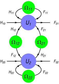
Figure 2: A unitary network with two nodes. Some of the connections may be absent.

Several unitary operators can be contracted to form a network. This is illustrated in Fig. 2 for a network with two nodes.

Definition 2  (Unitary network)  Let $U_{\alpha}:{\mathcal{H}}^{(\alpha)}\to{\mathcal{F}}^{(\alpha)}$, with $\alpha\in\{1,\ldots,N\}$ be a finite set of unitary operators. The spaces admit the decompositions

$${\mathcal{H}}^{(\alpha)}=\vbox{\hbox{\scalebox{1.1}{$\bigoplus$}}}_{\beta=0}^{N}{\mathcal{H}}_{\alpha\beta},\quad{\mathcal{F}}^{(\alpha)}=\vbox{\hbox{\scalebox{1.1}{$\bigoplus$}}}_{\beta=0}^{N}{\mathcal{F}}_{\beta\alpha},\quad\alpha\in\{1,\ldots,N\}\,.$$ (66)

Further

$$\varOmega_{\alpha\beta}:{\mathcal{F}}_{\alpha\beta}\to{\mathcal{H}}_{\alpha\beta},\qquad\alpha,\beta\in\{1,\ldots,N\}$$ (67)

are unitary maps. The unitary network is defined as the contraction $\varOmega\cdot U:{\mathcal{H}}_{0}\to{\mathcal{F}}_{0}$, where

$$U:=\vbox{\hbox{\scalebox{1.1}{$\bigoplus$}}}_{\alpha=1}^{N}U_{\alpha},\qquad\varOmega:=\vbox{\hbox{\scalebox{1.1}{$\bigoplus$}}}_{\alpha,\beta=1}^{N}\varOmega_{\alpha\beta}.$$ (68)

In this contraction

$$\begin{split}{\mathcal{H}}&=\vbox{\hbox{\scalebox{1.1}{$\bigoplus$}}}_{\alpha=1}^{N}{\mathcal{H}}^{(\alpha)},\qquad{\mathcal{F}}=\vbox{\hbox{\scalebox{1.1}{$\bigoplus$}}}_{\alpha=1}^{N}{\mathcal{F}}^{(\alpha)},\\ {\mathcal{H}}_{0}&=\vbox{\hbox{\scalebox{1.1}{$\bigoplus$}}}_{\alpha=1}^{N}{\mathcal{H}}_{\alpha 0},\qquad{\mathcal{F}}_{0}=\vbox{\hbox{\scalebox{1.1}{$\bigoplus$}}}_{\alpha=1}^{N}{\mathcal{F}}_{0\alpha},\\ {\mathcal{H}}_{1}&=\vbox{\hbox{\scalebox{1.1}{$\bigoplus$}}}_{\alpha,\beta=1}^{N}{\mathcal{H}}_{\alpha\beta},\qquad{\mathcal{F}}_{1}=\vbox{\hbox{\scalebox{1.1}{$\bigoplus$}}}_{\alpha,\beta=1}^{N}{\mathcal{F}}_{\alpha\beta}.\end{split}$$ (69)

$\diamondsuit$

The labels have been arranged with the convention that in $\alpha\beta$ the flow goes from $\beta$ to $\alpha$. Note that some (or even most) of the subspaces may vanish, that is, the graph needs not be complete. Due to unitarity of $U$’s and $\varOmega$’s, the following conditions on the dimension must be met:

$$\begin{split}&\dim{\mathcal{H}}_{\alpha\beta}=\dim{\mathcal{F}}_{\alpha\beta}\qquad\alpha,\beta>0\,,\\ &\sum_{\beta\geq 0}\dim{\mathcal{H}}_{\alpha\beta}=\sum_{\beta\geq 0}\dim{\mathcal{F}}_{\beta\alpha}\qquad\alpha>0\,.\end{split}$$ (70)

III Application to quantum graphs

In this section we apply the contraction of unitary operators to the scattering matrix of quantum graphs Kottos:1999 ; Kuchment:2008dub . We first consider a topological graph with a nonempty set $V^{\prime}$ of vertices and a nonempty set $E$ of edges, each edge joining two vertices. $|V^{\prime}|$ and $|E|$ are finite and no vertices of degree (valence) $0$ are allowed. Momentarily it will suffice to consider connected graphs as the extension to disconnected graphs is straightforward.

The graph becomes a metric graph by assigning to each edge a positive length that may be finite or infinite. The finite- and infinite-length edges will be referred to as internal and external lines, respectively. Correspondingly $E=E_{\rm i}\cup E_{\rm e}$, $E_{\rm i}\cap E_{\rm e}=\emptyset$. In the metric graph each line is a mathematical line, a connected one-dimensional real smooth manifold, endowed with a metric, and the points of the line belong to the metric graph.

There are two types of vertices, $V^{\prime}=V\cup V_{\infty}$, $V\cap V_{\infty}=\emptyset$. The vertices in $V_{\infty}$ represent points at infinity and have degree exactly one. All the points at infinity are regarded as different. $V$ are the finite or regular vertices. The internal lines have two vertices in $V$ as endpoints. For these an orientation is arbitrarily adopted so that one of the vertices is the initial endpoint of the line and the other is the final endpoint. Each point on the line $e\in E_{\rm i}$ has a coordinate $x$ which the distance to the initial endpoint and $x\in[0,l_{e}]$ where $l_{e}$ is the finite length of the internal line.

External lines may have one or two endpoints in $V_{\infty}$. The latter possibility would imply $|E_{\rm e}|=1$, $|V|=|E_{\rm i}|=0$ and will be disregarded. Therefore we assume that all external lines are of semi-infinite type, with one endpoint in $V$ and another in $V_{\infty}$ (hence $|V|>0$). These lines admit a canonical orientation, namely, from the regular vertex to the point at infinity. The coordinate $x$ on the external line is the distance to the regular-vertex endpoint and $x\in[0,+\infty)$.

Given a metric graph $\Gamma$, complex functions $f:\Gamma\to\mathbb{C}$ can be defined, $p\mapsto f(p)$ where $p$ is any point on an internal or external line, including the vertices. Here $\Gamma$ is regarded as a set including the interior points in the lines and the regular vertices, but not the points at infinity. The endpoints of different lines converging to a common vertex are identified as a single point of the metric graph as a set. Then a Hilbert space $L_{2}(\Gamma)$ can be defined. It is the orthogonal direct sum of all $L_{2}(e)$, the measurable and square integrable functions on the edge $e$,

$$\|f\|^{2}:=\sum_{e\in E}\int_{0}^{l_{e}}|f_{e}(x)|^{2}dx\leq+\infty.$$ (71)

In its simpler version, the quantum graph is obtained by considering a non relativistic quantum particle that moves on the metric graph. $\psi(p)$, $p\in\Gamma$, denotes its wavefunction. This requires introducing a quantum Hamiltonian $H$ as a suitable self-adjoint operator acting in $L_{2}(\Gamma)$.

We will only consider the potential-free case, hence on each line $e$ the Hamiltonian operator is just $\displaystyle-\frac{d^{2}}{dx^{2}}$ for interior points, with domain the Sobolev space $H^{2}(e)$. Appropriate boundary conditions should be given on the regular vertices to ensure self-adjointness. For each vertex $v\in V$ the boundary conditions take the form

$$A_{v}\Psi(v)+B_{v}\Psi^{\prime}(v)=0.$$ (72)

Here $\Psi(v)$ is the $d_{v}$-dimensional column vector of values of $\psi_{e}(v)$, which are the wavefunctions at $p=v$ along the lines $e$ with endpoints at $v$, and $d_{v}$ is the degree of the vertex $v$. The column vector $\Psi^{\prime}(v)$ contains $\psi^{\prime}_{e}(v)$, the derivatives with respect to the distance to the vertex. $A_{v}$ and $B_{v}$ are $d_{v}\times d_{v}$ constant complex matrices. Then the Hamiltonian operator is self-adjoint if and only if i) the $d_{v}\times 2d_{v}$ matrix $(A_{v},B_{v})$ has rank $d_{v}$, and ii) the matrix $A_{v}B_{v}^{\dagger}$ is Hermitian Berkolaiko:2013 .

Let $L:=|E_{\rm e}|=|V_{\infty}|$ be the number of external lines. For a compact graph, i.e. $L=0$, the energy spectrum is discrete, however only the case $L>0$ will be considered as we are interested in the scattering problem. Even if there is no potential energy on the lines, the boundary conditions may introduce contact interaction in the vertices, so the energy spectrum may have a negative part. The scattering states have positive energy $k^{2}$ with $k>0$ and the spectrum will be degenerated in general. The eigenfunctions on each line $e\in E$ are of the form $ae^{ikx}+be^{-ikx}$, $a,b\in\mathbb{C}$, hence there are $2|E|$ free coefficients. However each vertex $v\in V$ puts $d_{v}$ conditions. The graph identity $L+2|E_{\rm i}|=\sum_{v\in V}d_{v}$ then implies that each eigenvalue $k^{2}$ has degeneracy $L$.

For $k>0$ let $\Psi(p)$ be the solution with wavefunctions $a_{e}e^{ikx}+b_{e}e^{-ikx}$ for every $e\in E_{\rm e}$. The solution is univocally determined by choosing $L$ values for the coefficients $b_{e}$, then the linear map

$$\forall e\in E_{\rm e}\qquad a_{e}=\sum_{e^{\prime}\in E_{\rm e}}S(k)_{ee^{\prime}}b_{e^{\prime}}.$$ (73)

defines the scattering matrix $S(k)$ of the quantum graph. This is a unitary $L\times L$ matrix.

The simplest graphs are stars graphs, with just one vertex and $L$ external lines. Since the wavefunctions on the lines are $a_{e}e^{ikx}+b_{e}e^{-ikx}$, the boundary conditions in (72), can be cast in matrix form as

$$A(a+b)+ikB(a-b)=0.$$ (74)

Solving $a=Sb$ leads to the scattering matrix for the star graph

$$S=(ikB+A)^{-1}(ikB-A).$$ (75)

The conditions stated previously on the matrices $A$ and $B$ guarantee that $ikB+A$ is a regular matrix and $S$ is unitary Berkolaiko:2013 .

The discussion can be extended to disconnected graphs, including compact components. The Hilbert space is the direct sum of the corresponding spaces and the Hamiltonian is the sum of Hamiltonians of each subgraph. Likewise the scattering matrix is the direct sum of the scattering matrices of the components (counting the compact components as $0$-dimensional).

Definition 3  (Contraction of a quantum graph)  For a quantum graph with $L\geq 2$, let $e_{1}$ and $e_{2}$ be two different external lines, with corresponding regular vertices $v_{1}$ and $v_{2}$ (which need not be different). A contracted graph is obtained by removing the two external lines (as well as the corresponding points at infinity) and adding a new internal line $e$ with vertices $v_{1}$ and $v_{2}$ and assigning a finite length $l_{e}$ to the new internal line. The contracted vertices may belong to different or the same connected component. The process decreases $L$ in two units. More generally, a number $r$ of pairs of external lines may be removed to be replaced by internal lines. In this case the number of external lines becomes $L-2r$ in the contracted graph. $\diamondsuit$

The contraction is fully specified by the choice of unordered pairs of different external lines and the lengths of the resulting internal lines. Consequently the same final graph is obtained when the contractions are carried out sequentially in any order.

For a quantum graph $\Gamma$ and given $k>0$, let $a_{j}e^{ikx}+b_{j}e^{-ikx}$, $\forall j\in E_{\rm e}$, be wavefunctions with energy $k^{2}$ on the external lines. The coefficients $b_{j}$ and $a_{j}$ are the amplitudes of the inward and outward waves, respectively. Let ${\mathcal{H}}$ be the Hilbert space isomorphic to $\mathbb{C}^{L}$ of the coefficients $b_{j}$, and similarly ${\mathcal{F}}$ the space of the coefficients $a_{j}$. The scattering matrix is then a unitary map $S:{\mathcal{H}}\to{\mathcal{F}}$.

Let us consider a contraction of $\Gamma$, with pairings of external lines $\{(j_{1},m_{1}),\ldots,(j_{r},m_{r})\}$ and lengths of the resulting internal lines $\{l_{1},\ldots,l_{r}\}$, where $2r\leq L$ is assumed. Then ${\mathcal{H}}={\mathcal{H}}_{0}\oplus{\mathcal{H}}_{1}$ and ${\mathcal{F}}={\mathcal{F}}_{0}\oplus{\mathcal{F}}_{1}$, where ${\mathcal{H}}_{1}$ contains the coefficients $b_{j_{\ell}}$ and $b_{m_{\ell}}$, $\ell\in\{1,\ldots,r\}$ and ${\mathcal{F}}_{1}$ contains the coefficients $a_{j_{\ell}}$ and $a_{m_{\ell}}$, i.e. those corresponding to the external lines to be contracted. $\dim{\mathcal{H}}_{1}=\dim{\mathcal{F}}_{1}=2r$. In turn ${\mathcal{H}}_{0}$ and ${\mathcal{F}}_{0}$ are spanned by the inward and outward coefficients of the uncontracted external lines. A $2r\times 2r$-dimensional matrix $\varOmega$ can be constructed as a direct sum of $r$  $2\times 2$ blocks, as follows

$$\varOmega=\vbox{\hbox{\scalebox{1.1}{$\bigoplus$}}}_{\ell=1}^{r}\begin{pmatrix}0&\omega_{\ell}\\ \omega_{\ell}&0\end{pmatrix},\qquad\omega_{\ell}:=e^{ikl_{\ell}}\quad\ell\in\{1,\ldots,r\}.$$ (76)

$\varOmega$ is a unitary operator from ${\mathcal{F}}_{1}$ to ${\mathcal{H}}_{1}$. The blocks connect the two spaces using the scheme

$$\begin{pmatrix}b_{j_{\ell}}\\ b_{m_{\ell}}\end{pmatrix}=\begin{pmatrix}0&\omega_{\ell}\\ \omega_{\ell}&0\end{pmatrix}\begin{pmatrix}a_{j_{\ell}}\\ a_{m_{\ell}}\end{pmatrix}\qquad\ell\in\{1,\ldots,r\}.$$ (77)

Let $\Gamma$ be a quantum graph with scattering matrix $S$, and let $\Gamma^{\,\prime}$ be the contracted graph with connections as specified in $\varOmega$, with scattering matrix $S^{\prime}$. Then $S^{\prime}=\varOmega\cdot S$.

Proof  Because the contraction of graphs and the contraction of unitary operators can be carried out sequentially it will be sufficient to consider the case $r=1$, i.e., just two different external lines $j,m\in E_{\rm e}$ are contracted, to yield an internal line of length $l$.

Let $S$ be the scattering matrix of the original graph $\Gamma$. (More precisely the original graph removing its compact components, which play no role for the scattering but introduce a discrete spectrum at positive energies.) Starting from the $2|E|$ free coefficients $a_{e},b_{e}$, $e\in E$, the boundary conditions at the vertices impose $\sum_{v\in V}d_{v}$ constraints, leaving $L$ unconstrained parameters, which can be chosen as the $b_{e}$, $e\in E_{\rm e}$. In the contracted graph $\Gamma^{\,\prime}$ the lines $j$ and $m$ are identified, this implies the identification of the corresponding wavefunctions:

$$a_{j}e^{ikx}+b_{j}e^{-ikx}=a_{m}e^{ik(l-x)}+b_{m}e^{-ik(l-x)}$$ (78)

where $x$ is the distance to the regular vertex of $j$. Therefore, the operator $S^{\prime}$ (the scattering matrix of $\Gamma^{\,\prime}$) is defined by the same equations as $S$ by adding the new constraints

$$b_{j}=a_{m}\omega,\qquad b_{m}=a_{j}\omega,\qquad\omega:=e^{ikl}.$$ (79)

All the coefficients corresponding to internal lines of $\Gamma$ are fully fixed by the equations, therefore we can retain explicitly just those of the external lines. Let us denote $\psi\in{\mathcal{H}}$ the column vector of the $L$ coefficients $a_{e}$, $e\in E_{\rm e}$, and similarly $\phi\in{\mathcal{F}}$ for the $b_{e}$. These vectors can be split as $\psi_{0}+\psi_{1}$ and $\phi_{0}+\phi_{1}$, where ${\mathcal{H}}_{1}$ refers to $b_{j}$ and $b_{m}$ and ${\mathcal{F}}_{1}$ to $a_{j}$ and $a_{m}$. Then the equations defining $S^{\prime}$ are

$$\phi_{0}+\phi_{1}=S(\psi_{0}+\psi_{1}),\qquad\psi_{1}=\varOmega\phi_{1},$$ (80)

where $\displaystyle\varOmega=\begin{pmatrix}0&\omega\\ \omega&0\end{pmatrix}$. In $\Gamma^{\,\prime}$ the scattering matrix is the map $\psi_{0}\to\phi_{0}$, thus $S^{\prime}=\varOmega\cdot S$. $\square$

Figure 3: Contraction of a graph. The external lines $4$ and $5$ are contracted and the new line is assigned a length $l$, so that the phase is $\omega=e^{ikl}$. The lines $1$, $2$ and $3$ remain external so they carry a label $E$, while $4$ and $5$ become internal and carry a label $I$.

An example of contraction is displayed in Fig. 3. Initially the scattering matrix has dimension $5$. The space can be split into an external sector, with label $E$, corresponding to lines $1$, $2$ and $3$, and a internal sector, with label $I$, corresponding to lines $4$ and $5$. The scattering matrix then gets decomposed into submatrices as

$$S=\begin{pmatrix}S_{EE}&S_{EI}\\ S_{IE}&S_{II}\end{pmatrix}.$$ (81)

In the present example the blocks $S_{EE}$, $S_{II}$, $S_{EI}$ and $S_{IE}$, have dimensions $3\times 3$, $2\times 2$, $3\times 2$ and $2\times 3$, respectively, while the matrix $\varOmega$ is $2\times 2$. From Theorem LABEL:th:5, and making use of (43), it follows that the scattering matrix of the contracted graph can be expressed as

$$S^{\prime}=S_{EE}+S_{EI}(\varOmega^{-1}-S_{II})^{-1}S_{IE}.$$ (82)

Of course this formula holds in general, not just in our example. A similar expression has been derived previously in Caudrelier:2009ay .

As we have noted above, every vertex defines a unitary scattering matrix (regarding the vertex as a star graph) and obviously every graph can be obtained through contraction of the star graphs defined by its vertices. Therefore, (82) provides the scattering matrix for an arbitrary graph.

IV Non unitary contractions

IV.1 Contraction of non-unitary operators

Under suitable conditions the notion of contraction of an operator with a suboperator can be extended to more general operators and spaces. Let ${\mathcal{H}}={\mathcal{H}}_{0}\oplus{\mathcal{H}}_{1}$ and ${\mathcal{F}}={\mathcal{F}}_{0}\oplus{\mathcal{F}}_{1}$ be complex and finite dimensional vector spaces (the direct sum no longer implies orthogonality) and let $A:{\mathcal{H}}\to{\mathcal{F}}$ and $B:{\mathcal{F}}_{1}\to{\mathcal{H}}_{1}$ be linear maps. Relations of the type $\dim{\mathcal{H}}=\dim{\mathcal{F}}$, etc, no longer need to hold. One can still pose the problem whether the equations

$$\begin{split}&\phi_{0}+\phi_{1}=A(\psi_{0}+\psi_{1}),\qquad\psi_{1}=B\phi_{1},\\ &\psi_{j}\in{\mathcal{H}}_{j},\quad\phi_{j}\in{\mathcal{F}}_{j},\quad j\in\{0,1\}\end{split}$$ (83)

with input $\psi_{0}$ and unknowns $\psi_{1}$, $\phi_{0}$ and $\phi_{1}$, define a linear map $\psi_{0}\to\phi_{0}$. At variance with the unitary case, for more general operators this is not always guaranteed.

Proposition 8  The following are necessary and sufficient conditions for the eqs. (83) to define a linear map $\psi_{0}\to\phi_{0}$:

• $F_{1}A{\mathcal{H}}_{0}\subseteq(I-F_{1}AB){\mathcal{F}}_{1}$  (existence)

• $F_{0}AB{\mathcal{V}}_{1}=0$  (uniqueness of $\phi_{0}$)

$H_{j}$ and $F_{j}$, for $j\in\{0,1\}$, denote the projectors onto ${\mathcal{H}}_{j}$ and ${\mathcal{F}}_{j}$, respectively, and

$${\mathcal{V}}_{1}:=\{\varphi_{1}\in{\mathcal{F}}_{1}~{}|~{}F_{1}AB\varphi_{1}=\varphi_{1}\}.$$ (84)

Proof  Upon projection of (83) onto ${\mathcal{F}}_{0}$ and ${\mathcal{F}}_{1}$, and elimination of $\psi_{1}$, the equations become

$$\phi_{0}=F_{0}A(\psi_{0}+B\phi_{1}),\qquad\phi_{1}=F_{1}A(\psi_{0}+B\phi_{1}).$$ (85)

From the second equation it follows that the condition i) is necessary and sufficient for the existence of $\phi_{1}$ for all $\psi_{0}$, and then of $\phi_{0}$, using the first equation. ${\mathcal{V}}_{1}$ is the kernel of the operator $(I-F_{1}AB):{\mathcal{F}}_{1}\to{\mathcal{F}}_{1}$. A component $\varphi_{1}\in{\mathcal{V}}_{1}$ introduces an additive ambiguity in $\phi_{1}$. When inserted in the first equation, condition ii) encodes that $\phi_{0}$ is independent of $\varphi_{1}$, and so unique. $\square$

Obviously both conditions are met when ${\mathcal{V}}_{1}=0$, so this a sufficient condition for eqs. (83) to define a map $\psi_{0}\to\phi_{0}$. While sufficient, this condition is not necessary, the unitary case providing a counterexample.

The requirement of existence and uniqueness of the map suggests a possible definition of the contraction $B\cdot A$, which would fulfill the relation

$$B\cdot A=F_{0}(I-ABF_{1})^{-1}AH_{0}\,.$$ (86)

But this is not the only possibility. The contraction in the unitary case was also achieved as the sum of a series. An iterative treatment of the eqs. (83) would take the form

$$\begin{split}A\psi_{0}&=\phi_{0}^{(1)}+\phi_{0}^{(1)},\\ AB\phi_{1}^{(n)}&=\phi_{0}^{(n+1)}+\phi_{1}^{(n+1)}\quad\forall n\geq 1,\\ \phi_{0}&=\sum_{n=1}^{\infty}\phi_{0}^{(n)},\qquad\phi_{1}=\sum_{n=1}^{\infty}\phi_{1}^{(n)}.\end{split}$$ (87)

Clearly when both series are absolutely convergent they produce a solution of the equations, and hence a well-defined map $\psi_{0}\to\phi_{0}$. By absolute convergence it is meant convergence of the series

$$\sum_{n=1}^{\infty}\|\phi_{1}^{(n)}\|$$ (88)

(and similarly for $\phi_{0}$) using any vector-norm in ${\mathcal{F}}$. The definition does not depend on the concrete norm chosen. This follows from the property of finite-dimensional vector spaces that for any other norm $\|~{}\|^{\prime}$, there exist a $K>0$ such that $\forall v\in{\mathcal{F}}~{}\|v\|^{\prime}\leq K\|v\|$. Another observation is that absolute convergence of $\phi_{1}$ automatically implies that of $\phi_{0}$, due to

$$\|\phi_{0}^{(n+1)}\|=\|F_{0}AB\phi_{1}^{(n)}\|\leq\|F_{0}AB\|\|\phi_{1}^{(n)}\|.$$ (89)

The two possible definitions of $B\cdot A$ (namely, by uniqueness of the solution of the equation with respect to $\phi_{0}$, and by absolute convergence of the series) are different in general. There are pairs $(A,B)$ such that the solution is unique for $\phi_{0}$ with a divergent series, and it is also possible to violate the condition ii) in Proposition IV.1 having an absolutely convergent series. We will adopt the definition of $B\cdot A$ based in series as the more useful one, giving up the requirement of uniqueness of the solution for $\phi_{0}$.

Definition 4  (Contraction of an operator with a suboperator)  The contraction $B\cdot A:{\mathcal{H}}_{0}\to{\mathcal{F}}_{0}$ is defined as the linear map $\psi_{0}\to\phi_{0}$ determined by eqs. (87) whenever the series defining $\phi_{1}$ is absolutely convergent. Such $\phi_{0}$ and $\phi_{1}$ solve eqs. (83). The existence of additional solutions of the equations with a different $\phi_{0}$ is not excluded. $\diamondsuit$

The series defining the contraction is compactly expressed in eq. (86).

Proposition 9  When it is well-defined, the contraction fulfills

$$B\cdot A=\lim_{n\to\infty}(F_{0}+ABF_{1})^{n}AH_{0}\,.$$ (90)

Proof  The relations $F_{j}F_{k}=\delta_{jk}F_{j}$  ($j,k\in\{0,1\}$)  yield the identity

$$(F_{0}+ABF_{1})^{n}AH_{0}=F_{1}(ABF_{1})^{n}AH_{0}+\sum_{k=0}^{n}F_{0}(ABF_{1})^{k}AH_{0}\,.$$ (91)

When $n\to\infty$, the first term in the RHS goes to $0$ due to the absolute convergence of the series for $\phi_{1}$ in eq. (87). The second term reproduces the series defining $\phi_{0}$. $\square$

A sufficient condition for the contraction $B\cdot A$ to be well-defined is the existence of a subspace ${\mathcal{W}}\subseteq{\mathcal{F}}_{1}$ with the following properties:

• $F_{1}A{\mathcal{H}}_{0}\subseteq{\mathcal{W}}$,

• $F_{1}AB{\mathcal{W}}\subseteq{\mathcal{W}}$,

• $\|(F_{1}AB)^{k}\|_{{\mathcal{W}}}<1$ for some $k\geq 1$, where $\|~{}\|_{{\mathcal{W}}}$ denotes the norm restricted to ${\mathcal{W}}$, and $\|~{}\|$ denotes the operator-norm induced by some vector-norm in ${\mathcal{F}}$.

Proof  Under the condition i) $\phi_{1}^{(1)}\in{\mathcal{W}}$ and ii) implies that $\phi_{1}^{(n)}\in{\mathcal{W}}$ $\forall n\geq 1$. Then iii) guarantees the geometric convergence of the series: for a general term $n=mk+r$, with $m,r\in\mathbb{Z}$ and $r\in\{0,\ldots,k-1\}$, then $\|(F_{1}AB)^{n}\|_{{\mathcal{W}}}\leq\|(F_{1}AB)^{k}\|_{{\mathcal{W}}}^{m}\|F_{1}AB\|_{{\mathcal{W}}}^{r}$, so each subseries $r=0,\ldots,k-1$ is absolutely convergent and $B\cdot A$ is well-defined. $\square$

When ${\mathcal{W}}={\mathcal{F}}_{1}$ necessarily ${\mathcal{V}}_{1}=0$, and uniqueness of the solution of eqs. (83) with respect to $\phi_{0}$ is also guaranteed.

IV.2 Contraction of quantum channels

Definition 5  (Quantum channel)  Let ${\mathcal{H}}$ and ${\mathcal{F}}$ be Hilbert spaces. Let ${\mathcal{L}}({\mathcal{H}})={\mathcal{H}}\otimes{\mathcal{H}}^{*}$ and ${\mathcal{L}}({\mathcal{F}})={\mathcal{F}}\otimes{\mathcal{F}}^{*}$ denote the linear operators (endomorphisms) in ${\mathcal{H}}$ and in ${\mathcal{F}}$, respectively. $T$ is a quantum channel from ${\mathcal{H}}$ to ${\mathcal{F}}$ when it is a linear map $T:{\mathcal{L}}({\mathcal{H}})\to{\mathcal{L}}({\mathcal{F}})$ (a superoperator) that is completely positive (CP) and trace preserving (TP). $\diamondsuit$

In order to extend the concept of contraction to quantum channels, let ${\mathcal{H}}={\mathcal{H}}_{0}\oplus{\mathcal{H}}_{1}$ and ${\mathcal{F}}={\mathcal{F}}_{0}\oplus{\mathcal{F}}_{1}$, and let $T:{\mathcal{L}}({\mathcal{H}})\to{\mathcal{L}}({\mathcal{F}})$ and $R:{\mathcal{L}}({\mathcal{F}}_{1})\to{\mathcal{L}}({\mathcal{H}}_{1})$ be quantum channels. $T$ is the CPTP superoperator to be contracted and $R$ the connection and we would like to give a meaning to the contraction $R\cdot T$, as a quantum channel from ${\mathcal{H}}_{0}$ to ${\mathcal{F}}_{0}$.

A natural desideratum would be to demand that when $T$ and $R$ are unitary channels, corresponding to unitary maps $U$ and $\varOmega$, $R\cdot T$ would be a unitary quantum channel for $\varOmega\cdot U$, however, this requirement cannot be met. To be more specific, let us introduce the notation Cai:2019

$$\overbracket{A}(~{}):=A(~{})A^{\dagger},$$ (92)

where $A$ is an operator and so $\overbracket{A}$ is a superoperator. The symbol fulfills the property $\overbracket{AB}=\overbracket{A}\,\overbracket{B}$. By definition, $T$ is a unitary quantum channel for the unitary operator $U$ when $T=\overbracket{U}$, that is, $T(\rho)=U\rho U^{\dagger}$. Likewise $R=\overbracket{\varOmega}$. Then the requirement (where the LHS is yet to be defined)

$$\overbracket{\varOmega}\cdot\overbracket{U}=\overbracket{\varOmega\cdot U}$$ (93)

is inconsistent, because $\overbracket{U}$ and $\overbracket{\varOmega}$ are invariant under $U\to\omega U$, $\varOmega\to\omega^{\prime}\varOmega$ ($\omega,\omega^{\prime}\in\mathbb{C}$ and $|\omega|=|\omega^{\prime}|=1$) while $\overbracket{\varOmega\cdot U}$ is not, unless $\omega^{\prime}=\omega^{*}$. (In general $(\omega^{\prime}\varOmega)\cdot(\omega U)$ is not $\omega^{\prime\prime}(\varOmega\cdot U)$.)

A possible definition for $R\cdot T$ comes from Stinespring’s dilation theorem Paulsen:2003 , which associates every CPTP superoperator to a unitary operator in an extended Hilbert space. Unfortunately the unitary operators $U$ and $\varOmega$ corresponding to $T$ and $R$ are not unique and the different choices would yield different results for $\varOmega\cdot U$. Therefore the definition of $R\cdot T$ would not depend solely on the channel $T$ and the subchannel $R$. So we disregard this approach.

Let us decompose ${\mathcal{L}}({\mathcal{H}})$ into the four sectors,

$${\mathcal{L}}({\mathcal{H}})={\mathcal{H}}_{0}\otimes{\mathcal{H}}_{0}^{*}\oplus{\mathcal{H}}_{0}\otimes{\mathcal{H}}_{1}^{*}\oplus{\mathcal{H}}_{1}\otimes{\mathcal{H}}_{0}^{*}\oplus{\mathcal{H}}_{1}\otimes{\mathcal{H}}_{1}^{*},$$ (94)

and similarly for ${\mathcal{L}}({\mathcal{F}})$. Then, the operators $\rho\in{\mathcal{L}}({\mathcal{H}})$ and $\sigma\in{\mathcal{L}}({\mathcal{F}})$ admit the decompositions

$$\begin{split}\rho&=\rho_{00}+\rho_{01}+\rho_{10}+\rho_{11},\\ \sigma&=\sigma_{00}+\sigma_{01}+\sigma_{10}+\sigma_{11}.\end{split}$$ (95)

In analogy with (83), we can pose the problem whether, for given $T$ and $R$, and $\rho_{00}$, the equations

$$\sigma=T(\rho),\qquad R(\sigma_{11})=\rho_{11},\qquad\rho_{01}=\rho_{10}=0,$$ (96)

have a solution for $\rho_{01}$, $\rho_{10}$, $\rho_{11}$, $\sigma_{00}$, $\sigma_{01}$, $\sigma_{10}$ and $\sigma_{11}$, unique for $\sigma_{00}$, hence providing a well-defined linear map $\rho_{00}\to\sigma_{00}$.

Note that choices have been made in writing the equations in (96), namely, the conditions $\rho_{01}=\rho_{10}=0$. This is necessary (or at least convenient) to match the number of unknowns with that of equations. The choice taken corresponds to the iterative process to be set up below, in (104). The equations (96) do not distinguish between a quantum channel $T$ and its “decohered” version $T^{\prime}$

$$T^{\prime}:=(\overbracket{F_{0}}+\overbracket{F_{1}})\vbox{\hbox{\scalebox{0.7}{$\circ$}}}T\vbox{\hbox{\scalebox{0.7}{$\circ$}}}(\overbracket{H_{0}}+\overbracket{H_{1}}).$$ (97)

(As before, $H_{j}$ and $F_{j}$, with $j\in\{0,1\}$, denote orthogonal projectors.) $T^{\prime}$ is also a quantum channel which only attends to the diagonal sectors of $T$. That is,

$$T^{\prime}(\rho_{01}+\rho_{10})=0$$ (98)

and

$$\sigma_{00}+\sigma_{11}=T^{\prime}(\rho_{00}+\rho_{11})$$ (99)

when

$$\sigma_{00}+\sigma_{01}+\sigma_{10}+\sigma_{11}=T(\rho_{00}+\rho_{11}),$$ (100)

Therefore any information related to coherence between the spaces ${\mathcal{H}}_{0}$ and ${\mathcal{H}}_{1}$, or ${\mathcal{F}}_{0}$ and ${\mathcal{F}}_{1}$ is lost in the map $\rho_{00}\to\sigma_{00}$ defined by (96). It follows that the set of solutions for the pairs $(T,R)$ or $(T^{\prime},R)$ are identical.

Since the off-diagonal spaces ${\mathcal{H}}_{0}\otimes{\mathcal{H}}_{1}^{*}$, ${\mathcal{H}}_{1}\otimes{\mathcal{H}}_{0}^{*}$, ${\mathcal{F}}_{0}\otimes{\mathcal{F}}_{1}^{*}$ and ${\mathcal{F}}_{1}\otimes{\mathcal{F}}_{0}^{*}$ do not play a role, in what follows we will use the notation $\rho_{0}$ (for $\rho_{00}$) and $\sigma_{0}$ and $\sigma_{1}$ (for $\sigma_{00}$ and $\sigma_{11}$ respectively). In this way (96) can be expressed as

$$\begin{split}&\sigma_{0}+\sigma_{1}=T^{\prime}(\rho_{0}+\rho_{1}),\qquad R(\sigma_{1})=\rho_{1},\\ &\rho_{j}\in{\mathcal{L}}({\mathcal{H}}_{j}),\quad\sigma_{j}\in{\mathcal{L}}({\mathcal{F}}_{j})\quad j\in\{0,1\}.\end{split}$$ (101)

It must be noted that, unlike what happened in the contraction of unitary operators, that $T$ and $R$ are quantum channels does not guarantee that eqs. (101) have a solution. A counterexample is readily found: let ${\mathcal{H}}={\mathcal{F}}=\mathbb{C}^{2}$, with ${\mathcal{H}}_{0}={\mathcal{F}}_{0}=\{(z,0)~{}|~{}z\in\mathbb{C}\}$, $R$ the identity map and

$$T(\rho):=\operatorname{Tr}(\rho)H_{1}\,.$$ (102)

As can be verified, for such $T$ and $R$, eqs. (101) are inconsistent unless $\rho_{0}=0$.

Even though eqs. (101) are formally identical to eqs. (83) (viewing the quantum channels $T^{\prime}$ and $R$ as (super)operators, and the operators $\rho$ and $\sigma$ as (super)vectors) the treatment cannot be identical due to the additional requirement that the linear map $\rho_{0}\to\sigma_{0}$ must be CP (as well as TP, but this is a straightforward consequence of the equations). Positivity is a crucial issue in the context of quantum channels, and the treatment has to be adapted accordingly.

For convenience, out of $T$ and $R$, we define the following CP superoperators,

$$\begin{split}T_{j0}&:=\overbracket{F_{j}}\vbox{\hbox{\scalebox{0.7}{$\circ$}}}T\vbox{\hbox{\scalebox{0.7}{$\circ$}}}\overbracket{H_{0}}:{\mathcal{L}}({\mathcal{H}}_{0})\to{\mathcal{L}}({\mathcal{F}}_{j}),\qquad\\ \tilde{T}_{j1}&:=\overbracket{F_{j}}\vbox{\hbox{\scalebox{0.7}{$\circ$}}}T\vbox{\hbox{\scalebox{0.7}{$\circ$}}}R:{\mathcal{L}}({\mathcal{F}}_{1})\to{\mathcal{L}}({\mathcal{F}}_{j}),\qquad j\in\{0,1\}.\end{split}$$ (103)

Note that $T_{00}+T_{10}$ and $\tilde{T}_{01}+\tilde{T}_{11}$ are both CPTP, and also that the same operators are produced using $T^{\prime}$ instead of $T$. An iterative treatment, aiming to a series solution of eqs. (101), produces

$$\begin{split}\sigma_{0}^{(1)}&=T_{00}(\rho_{0}),\qquad\sigma_{1}^{(1)}=T_{10}(\rho_{0}),\\ \sigma_{0}^{(n+1)}&=\tilde{T}_{01}(\sigma_{1}^{(n)}),\qquad\sigma_{1}^{(n+1)}=\tilde{T}_{11}(\sigma_{1}^{(n)})\quad\forall n\geq 1,\\ \sigma_{0}&=\sum_{n=1}^{\infty}\sigma_{0}^{(n)},\qquad\sigma_{1}=\sum_{n=1}^{\infty}\sigma_{1}^{(n)}.\end{split}$$ (104)

If $\rho_{0}$ is a positive operator (more precisely, a non-negative operator, $\rho_{0}\geq 0$) the operators $\sigma_{0}^{(n)}$ and $\sigma_{1}^{(n)}$ are all positive too. If both series in (104) are absolutely convergent, $\sigma_{0}$ and $\sigma_{1}$ provide a solution to (101) and a well-defined positive linear map $\rho_{0}\to\sigma_{0}$.

In order to give a precise meaning to the convergence of the series, the operator-norm induced in ${\mathcal{L}}({\mathcal{F}})$ by the Hilbert space-norm is not a natural one for quantum channels. Instead the trace is more appropriate. To this end we introduce the following definition:

Definition 6  For positive operators $\rho\in{\mathcal{L}}({\mathcal{H}})$ (actually non-negative, $\rho\geq 0$) let $\|\rho\|_{t}:=\operatorname{Tr}(\rho)$. The function $\|~{}\|_{t}$ enjoys the required properties of a norm: $\|\rho\|_{t}\geq 0$ and $\|\rho\|_{t}=0$ only if $\rho=0$, and $\|\lambda\rho\|_{t}=\lambda\|\rho\|_{t}$ for $\lambda\geq 0$, as well as $\|\rho+\sigma\|_{t}=\|\rho\|_{t}+\|\sigma\|_{t}$. In turn, this induces a norm on positive superoperators. For a linear $T:{\mathcal{L}}({\mathcal{H}})\to{\mathcal{L}}({\mathcal{F}})$ and $T\geq 0$,

$$\|T\|_{t}:=\sup\{\operatorname{Tr}(T(\rho))~{}|~{}\forall\rho\in{\mathcal{L}}({\mathcal{H}}),~{}\rho\geq 0,~{}\operatorname{Tr}(\rho)=1\}.$$ (105)

This induced norm has the basic properties $\|T_{1}\vbox{\hbox{\scalebox{0.7}{$\circ$}}}T_{2}\|_{t}\leq\|T_{1}\|_{t}\|T_{2}\|_{t}$ and $\|T_{1}+T_{2}\|_{t}\leq\|T_{1}\|_{t}+\|T_{2}\|_{t}$. $\diamondsuit$

With this definition $\|T\|_{t}=1$ when $T$ is a quantum channel.

Lemma 4  Let $E^{(i)}:{\mathcal{L}}({\mathcal{H}})\to{\mathcal{L}}({\mathcal{F}})$, $i\in\{1,\ldots,n\}$, be completely positive superoperators, and $E=\sum_{i=1}^{n}E^{(i)}$ a quantum channel. Let $S^{(i)}:{\mathcal{L}}({\mathcal{F}})\to{\mathcal{L}}({\mathcal{G}})$, $i\in\{1,\ldots,n\}$, be quantum channels. Then

$$T=\sum_{i=1}^{n}S^{(i)}\vbox{\hbox{\scalebox{0.7}{$\circ$}}}E^{(i)}$$ (106)

is a quantum channel.

Proof  The composition and sum of completely positive operators is completely positive. Regarding the preservation of the trace

$$\begin{split}\operatorname{Tr}_{{\mathcal{G}}}(T(\rho))&=\sum_{i=1}^{n}\operatorname{Tr}_{{\mathcal{G}}}(S^{(i)}(E^{(i)}(\rho)))=\sum_{i=1}^{n}\operatorname{Tr}_{{\mathcal{F}}}(E^{(i)}(\rho))\\ &=\operatorname{Tr}_{{\mathcal{F}}}(E(\rho))=\operatorname{Tr}_{\mathcal{H}}(\rho).\end{split}$$ (107)

$\square$

Proposition 10  If the series of $\sigma_{1}$ in eqs. (104) is absolutely convergent (in the sense of the norm $\|~{}\|_{t}$):

• The series of $\sigma_{0}$ is also absolutely convergent.

• The map $\rho_{0}\to\sigma_{0}$ is CPTP.

Proof  The assertion i) follows from

$$\|\sigma_{0}^{(n+1)}\|_{t}=\|\tilde{T}_{01}(\sigma_{1}^{(n)})\|_{t}\leq\|\tilde{T}_{01}\|_{t}\|\sigma_{1}^{(n)}\|_{t}.$$ (108)

To prove ii), let us establish the relation (provisionally denoting $R\cdot T$ the map $\rho_{0}\to\sigma_{0}$)

$$R\cdot T=\lim_{n\to\infty}\tilde{T}^{n}\vbox{\hbox{\scalebox{0.7}{$\circ$}}}T^{\prime}\vbox{\hbox{\scalebox{0.7}{$\circ$}}}\overbracket{H_{0}},\qquad\tilde{T}:=\overbracket{F_{0}}+T^{\prime}\vbox{\hbox{\scalebox{0.7}{$\circ$}}}R\vbox{\hbox{\scalebox{0.7}{$\circ$}}}\overbracket{F_{1}}\,.$$ (109)

The repeated application of $\tilde{T}$ produces

$$\rho_{0}\to\tilde{T}^{n}\vbox{\hbox{\scalebox{0.7}{$\circ$}}}T^{\prime}(\rho_{0})=\sum_{k=1}^{n}\sigma_{0}^{(k)}+\sigma_{1}^{(n)}\quad\forall n\geq 1.$$ (110)

By Lemma IV.2, $\tilde{T}$ is a quantum channel, hence for finite $n$, $\tilde{T}^{n}\vbox{\hbox{\scalebox{0.7}{$\circ$}}}T^{\prime}\vbox{\hbox{\scalebox{0.7}{$\circ$}}}\overbracket{H_{0}}$ is a quantum channel from ${\mathcal{H}}_{0}$ to ${\mathcal{F}}$. The limit exists due to the absolute convergence, and yields the map $\rho_{0}\to\sigma_{0}$ which is then a quantum channel from ${\mathcal{H}}_{0}$ to ${\mathcal{F}}_{0}$. $\square$

We can now give a proper definition for the contraction $R\cdot T$,

Definition 7  (Contraction of quantum channels)  Given $T$ and $R$, and $\rho_{0}$, the contraction $R\cdot T$ is defined as the map $\rho_{0}\to\sigma_{0}$ determined by eqs. (104), provided the series for $\sigma_{1}$ is absolutely convergent in the sense of $\|~{}\|_{t}$. By Proposition IV.2 this property guarantees that $\sigma_{0}$ is also absolutely convergent and the map $\rho_{0}\to\sigma_{0}$ is a quantum channel.

Clearly with this definition the contraction depends only on $T$ and $R$ themselves, and $R\cdot T=R\cdot T^{\prime}$. Also, the $\rho$ and $\sigma$ defined by the series solve eqs. (101). $\diamondsuit$

The series defining the contraction can be expressed as

$$R\cdot T=T_{00}+\tilde{T}_{01}\vbox{\hbox{\scalebox{0.7}{$\circ$}}}(I+\tilde{T}_{11}+\tilde{T}_{11}^{2}+\tilde{T}_{11}^{3}+\cdots)\vbox{\hbox{\scalebox{0.7}{$\circ$}}}T_{10},$$ (111)

or more compactly as

$$\begin{split}R\cdot T&=T_{00}+\tilde{T}_{01}\vbox{\hbox{\scalebox{0.7}{$\circ$}}}(I-\tilde{T}_{11})^{-1}\vbox{\hbox{\scalebox{0.7}{$\circ$}}}T_{10}\\ &=\overbracket{F_{0}}\vbox{\hbox{\scalebox{0.7}{$\circ$}}}(I-T\vbox{\hbox{\scalebox{0.7}{$\circ$}}}R\vbox{\hbox{\scalebox{0.7}{$\circ$}}}\overbracket{F_{1}})^{-1}\vbox{\hbox{\scalebox{0.7}{$\circ$}}}T\vbox{\hbox{\scalebox{0.7}{$\circ$}}}\overbracket{H_{0}},\end{split}$$ (112)

A sufficient condition for the contraction $R\cdot T$ to be well-defined is the existence of a subspace $\hat{{\mathcal{W}}}\subseteq{\mathcal{L}}({\mathcal{F}}_{1})$ with the following properties:

• $T_{10}{\mathcal{L}}({\mathcal{H}}_{0})\subseteq\hat{{\mathcal{W}}}$,

• $\tilde{T}_{11}\hat{{\mathcal{W}}}\subseteq\hat{{\mathcal{W}}}$,

• $\|(\tilde{T}_{11})^{k}\|_{t,\hat{{\mathcal{W}}}}<1$ for some $k\geq 1$, where $\|~{}\|_{t,\hat{{\mathcal{W}}}}$ denotes the norm $\|~{}\|_{t}$ restricted to $\hat{{\mathcal{W}}}$.

Proof  Conditions i) and ii) guarantee that $\sigma_{1}^{(n)}\in\hat{{\mathcal{W}}}$. Condition iii) guarantees a geometric convergence rate of the series. $\square$

Example 2  Let us consider a simple example. Let $U_{jk}^{(m)}:{\mathcal{H}}_{k}\to{\mathcal{F}}_{j}$, $\forall m\in I_{jk}$ (a finite index set) for $j,k\in\{0,1\}$, be unitary operators. And also unitary $\varOmega^{(n)}:{\mathcal{F}}_{1}\to{\mathcal{H}}_{1}$, $\forall n\in I^{\prime}$ (another finite index set). In addition, let

$$\begin{split}&p_{jk}^{(m)}\geq 0,\qquad q^{(n)}\geq 0,\qquad\bar{p}_{jk}:=\sum_{m}p_{jk}^{(m)},\qquad\\ &\bar{p}_{00}+\bar{p}_{10}=1,\qquad\bar{p}_{01}+\bar{p}_{11}=1,\qquad\sum_{n}q^{(n)}=1\end{split}$$ (113)

Then

$$T_{jk}:=\sum_{m}p_{jk}^{(m)}\overbracket{U_{jk}^{(m)}},\qquad T:=\sum_{j,k}T_{jk},\qquad R:=\sum_{n}q^{(n)}\overbracket{\varOmega^{(n)}}.$$ (114)

$R$ is a random unitary channel, i.e., convex combinations of unitary channels. $T$ is closely related to, but not exactly, a random unitary channel, as it is not a mixture of unitary operators ${\mathcal{H}}\to{\mathcal{F}}$ (except for special choices of the weights $p_{jk}^{(m)}$). $T$ has been chosen in such a way that $T=T^{\prime}$.

Eq. (101) corresponds to

$$\begin{split}\sigma_{0}&=\sum_{m}p_{00}^{(m)}\overbracket{U_{00}^{(m)}}\rho_{0}+\sum_{m}p_{01}^{(m)}\overbracket{U_{01}^{(m)}}\sum_{n}q^{(n)}\overbracket{\varOmega^{(n)}}\sigma_{1},\\ \sigma_{1}&=\sum_{m}p_{10}^{(m)}\overbracket{U_{10}^{(m)}}\rho_{0}+\sum_{m}p_{11}^{(m)}\overbracket{U_{11}^{(m)}}\sum_{n}q^{(n)}\overbracket{\varOmega^{(n)}}\sigma_{1}.\end{split}$$ (115)

Attending to the traced equations

$$\begin{split}\operatorname{Tr}(\sigma_{0})&=\bar{p}_{00}\operatorname{Tr}(\rho_{0})+\bar{p}_{01}\operatorname{Tr}(\sigma_{1}),\\ \operatorname{Tr}(\sigma_{1})&=\bar{p}_{10}\operatorname{Tr}(\rho_{0})+\bar{p}_{11}\operatorname{Tr}(\sigma_{1}),\end{split}$$ (116)

two cases can be distinguished:

• $\bar{p}_{11}=1$. Since we want a generic $\rho_{0}$, the system can only be consistent if $\bar{p}_{10}=0$. Then also $\bar{p}_{00}=1$, and $p_{01}^{(m)}=p_{10}^{(m)}=0$ $\forall m$. The two sectors $0$ and $1$ are decoupled. $T_{10}=0$ and the series converges in one step. $R\cdot T$ is just $T_{00}$.

• $\bar{p}_{11}<1$. In this case $\displaystyle\operatorname{Tr}(\sigma_{1})=\frac{\bar{p}_{10}}{\bar{p}_{01}}\operatorname{Tr}(\rho_{0})$. $\sigma_{1}$ is not bounded for fixed $\operatorname{Tr}(\rho_{0})$, but still $\operatorname{Tr}(\sigma_{0})=\operatorname{Tr}(\rho_{0})$ as it should. For the solution to the full (untraced) equations (115) the condition $\bar{p}_{11}<1$ ensures the convergence of the series for $\sigma_{1}$, or equivalently of that in (111). The latter expression shows that, in this example, $R\cdot T$ is a random unitary quantum channel (with an infinite, but convergent, Kraus representation).

$\diamondsuit$

The contraction of unitary quantum channels always produces a quantum channel:

Proposition 11  Let $U:{\mathcal{H}}_{0}\oplus{\mathcal{H}}_{1}\to{\mathcal{F}}_{0}\oplus{\mathcal{F}}_{1}$ and $\varOmega:{\mathcal{F}}_{1}\to{\mathcal{H}}_{1}$ be unitary operators. Then the contraction of the unitary quantum channels $\overbracket{\varOmega}$ and $\overbracket{U}$ exists and defines a quantum channel. Moreover,

$$\overbracket{\varOmega}\cdot\overbracket{U}=T_{U,\varOmega},$$ (117)

where $T_{U,\varOmega}$ is the quantum channel of eq. (60).

Proof  For $T=\overbracket{U}$ and $R=\overbracket{\varOmega}$, the operators defined in (103) take the form

$$\begin{split}T_{00}&=\overbracket{F_{0}}\vbox{\hbox{\scalebox{0.7}{$\circ$}}}\overbracket{U}\vbox{\hbox{\scalebox{0.7}{$\circ$}}}\overbracket{H_{0}}=\overbracket{U_{00}},\quad\\ \tilde{T}_{01}&=\overbracket{\tilde{U}_{01}},\quad T_{10}=\overbracket{U_{10}},\quad\tilde{T}_{11}=\overbracket{\tilde{U}_{11}},\end{split}$$ (118)

where the notation $U_{00}$, $\tilde{U}_{01}$, $U_{10}$ and $\tilde{U}_{11}$ was introduced in (44). For the contraction $\overbracket{\varOmega}\cdot\overbracket{U}$ to exist, the series for $\sigma_{1}$ in (104) must be absolutely convergent for any $\rho_{0}\in{\mathcal{L}}({\mathcal{H}}_{0})$. By linearity, it is sufficient to show this for a $\rho_{0}$ of the form (a pure state)

$$\rho_{0}=\psi_{0}\otimes\psi_{0}^{\dagger}:=\overbracket{\psi_{0}},\qquad\psi_{0}\in{\mathcal{H}}_{0}$$ (119)

where $\psi_{0}^{\dagger}$ is the canonical form dual to $\psi_{0}$ (under the Hilbert space scalar product), and we have introduced the notation $\overbracket{\psi}:=\psi\otimes\psi^{\dagger}$ for vectors, then

$$\|\overbracket{\psi}\|_{t}=\|\psi\|^{2}.$$ (120)

For those $\rho_{0}$ the relation

$$\sigma_{1}^{(n)}=\tilde{T}_{11}^{n-1}T_{10}(\rho_{0})\quad\forall n\geq 1$$ (121)

becomes

$$\sigma_{1}^{(n)}=\overbracket{\tilde{U}_{11}^{n-1}U_{10}\psi_{0}}=\overbracket{\phi_{1}^{(n)}}\quad\forall n\geq 1,$$ (122)

where $\phi_{1}^{(n)}$ is that of (52). Hence

$$\|\sigma_{1}^{(n)}\|_{t}=\|\phi_{1}^{(n)}\|^{2}.$$ (123)

The absolute convergence of the quantum channels series then follows from that already established for the contraction of unitary operators. This shows that $\overbracket{\varOmega}\cdot\overbracket{U}$ exists.

Along the same lines, it is straightforward to verify that

$$\sigma_{0}^{(n)}=\overbracket{\phi_{0}^{(n)}}=\overbracket{A_{n}}(\rho_{0})\quad\forall n\geq 1.$$ (124)

This implies that

$$\overbracket{\varOmega}\cdot\overbracket{U}=\sum_{n=1}^{\infty}\overbracket{A_{n}}=T_{U,\varOmega}.$$ (125)

$\square$

The following nice relations have then been obtained:

$$\varOmega\cdot U=\sum_{n=1}^{\infty}A_{n},\qquad\overbracket{\varOmega}\cdot\overbracket{U}=\sum_{n=1}^{\infty}\overbracket{A_{n}}\,.$$ (126)

Proposition IV.2 will be invoked in Sec. V.

Let $\hat{{\mathcal{V}}}\subseteq{\mathcal{L}}({\mathcal{F}}_{1})$ denote the largest positive subspace which is invariant under $T^{\prime}\vbox{\hbox{\scalebox{0.7}{$\circ$}}}R$. By positive subspace we mean spanned by positive operators. The invariance implies $\tilde{T}_{11}\hat{{\mathcal{V}}}\subseteq\hat{{\mathcal{V}}}$ and $\tilde{T}_{01}\hat{{\mathcal{V}}}=0$, and also that $\tilde{T}_{11}$ is a quantum channel when restricted to ${\mathcal{V}}$. Clearly, if some non-null component of $\sigma_{1}^{(n)}$ ever enters into $\hat{{\mathcal{V}}}$, such component will remain there and the series will not converge. To be more specific, let us assume that for some $n$ during the iteration (104),

$$\sigma_{1}^{(n)}=\sigma_{W}+\sigma_{V},\qquad\sigma_{W}\geq 0,\quad\sigma_{V}\geq 0,\qquad 0\neq\sigma_{V}\in\hat{{\mathcal{V}}}.$$ (127)

Then $\|\sigma_{V}\|_{t}>0$. Since $\tilde{T}_{11}$ is CP in ${\mathcal{L}}({\mathcal{F}}_{1})$ and CPTP within $\hat{{\mathcal{V}}}$,

$$\begin{split}\|\sigma_{1}^{(n+k)}\|_{t}&=\|\tilde{T}_{11}^{k}(\sigma_{W})\|_{t}+\|\tilde{T}_{11}^{k}(\sigma_{V})\|_{t}\\ &=\|\tilde{T}_{11}^{k}(\sigma_{W})\|_{t}+\|\sigma_{V}\|_{t}\geq\|\sigma_{V}\|_{t}\quad\forall k\geq 0.\end{split}$$ (128)

It follows that the series of $\sigma_{1}$ will not converge.

Lemma 5  When ${\mathcal{L}}({\mathcal{F}}_{1})\neq 0$, $\hat{{\mathcal{V}}}=0$ if and only if $\|(\tilde{T}_{11})^{d}\|_{t}<1$, where $d:=\dim{\mathcal{L}}({\mathcal{F}}_{1})$.

Proof  Suppose $\hat{{\mathcal{V}}}\neq 0$. The superoperators $\tilde{T}_{11}^{n}$, $n\geq 0$, are all quantum channels when restricted to $\hat{{\mathcal{V}}}$, then $\|(\tilde{T}_{11})^{n}\|_{t}=1$ for all $n\geq 0$. Now suppose $\|(\tilde{T}_{11})^{d}\|_{t}=1$. Then $\exists\sigma^{(0)}\in{\mathcal{L}}({\mathcal{F}}_{1})$, $\sigma^{(0)}\geq 0$, $\operatorname{Tr}(\sigma^{(0)})=1$, such that $\operatorname{Tr}(\tilde{T}_{11}^{d}(\sigma^{(0)}))=1$. Let $\sigma^{(k)}:=\tilde{T}_{11}^{k}(\sigma^{(0)})$, $0\leq k\leq d$. Since $\|\tilde{T}_{11}\|_{t}\leq 1$, necessarily $\operatorname{Tr}(\sigma^{(k)})=1$, and $\sigma^{(k)}\geq 0$ for $0\leq k\leq d$. As no $d+1$ operators can be linearly independent in ${\mathcal{L}}({\mathcal{F}}_{1})$, $\sigma^{(k_{0})}$, for some $0<k_{0}\leq d$, must be a linear combination of the previous $\sigma^{(k)}$ ($0\leq k<k_{0}$). Such $k_{0}$ positive operators span a non-zero invariant and positive subspace of ${\mathcal{L}}({\mathcal{F}}_{1})$, hence $\hat{{\mathcal{V}}}\neq 0$. $\square$

Corollary 2 $\hat{{\mathcal{V}}}=0$ is a sufficient condition for $R\cdot T$ to exist.

Proof  If ${\mathcal{L}}({\mathcal{F}}_{1})=0$ the series (104) converges in one step. If ${\mathcal{L}}({\mathcal{F}}_{1})\neq 0$ and $\hat{{\mathcal{V}}}=0$, Lemma IV.2 implies that $\|(\tilde{T}_{11})^{d}\|_{t}<1$ for a $d\geq 1$, hence $R\cdot T$ exists from Theorem LABEL:th:7 with $\hat{{\mathcal{W}}}={\mathcal{L}}({\mathcal{F}}_{1})$. $\square$

We have noted that the contraction of quantum channel with a subchannel does not always exist (e.g. case $\bar{p}_{11}=1$ with $\bar{p}_{00}<1$ in Example IV.2). However, the possibility that whenever eqs. (101) have a solution (perhaps with additional conditions) such solution must be a quantum channel, has not been discarded. This issue is not settled in this work.

V Implementation in quantum computation

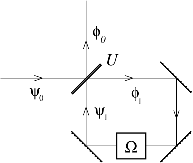
Figure 4: A unitary contraction implemented through a beam of stationary coherent light.

Fig. 4 illustrates a unitary contraction implemented through a beam of stationary coherent light. We disregard the polarization degree of freedom as it does not play a role in this example. The incident beam with amplitude $\psi_{0}$ enters an ideal beam splitter with transmission and reflection coefficients $t$ and $r$, respectively, and associated unitary operator $\displaystyle U=\begin{pmatrix}t&r^{\prime}\\ r&t^{\prime}\end{pmatrix}$. Part of the amplitude of the beam is immediately reflected in the beam splitter (adding to $\phi_{0}$) and part transmitted (adding to $\phi_{1}$). The latter component, after reflecting on the mirrors returns to the splitter, again with the possibilities of transmission (to $\phi_{0}$) or reflection (to $\phi_{1}$). A phase shifter $\varOmega$ can be inserted in the loop. The equations constraining the amplitudes are then

$$\psi_{1}=\varOmega\phi_{1},\qquad\phi_{1}=t\psi_{0}+r^{\prime}\psi_{1},\qquad\phi_{0}=r\psi_{0}+t^{\prime}\psi_{1}.$$ (129)

The solution produces a linear relationship $\phi_{0}=S\psi_{0}$ where $S=\varOmega\cdot U$ is a phase identical to that already found in the Example II.1 with obvious identifications. The present illustration would correspond to a space ${\mathcal{H}}$ of a qubit (since the amplitude can arrive from two different directions to the beam splitter) with a decomposition $\mathbb{C}^{2}=\mathbb{C}\oplus\mathbb{C}$. Clearly an important problem arises if the setting is directly applied to a photon, due to the delay between the various components $\phi_{0}^{(n)}$ coming out of the splitter.

In all our previous discussions, with the exception of Proposition II.2, we have manipulated Hilbert spaces additively (direct sum of spaces) instead of multiplicatively (tensor product of spaces). The latter is characteristic of quantum computation, and is the reason of the efficiency of such approach when treating certain computational problems. The additive structure is natural for quantum graphs. There the dimension of the space increases linearly with the number of external lines of the graph. In the case of quantum circuits, the dimension increases exponentially with the number of qubits. It should be quite clear then that the contraction discussed in this work does not refer to closing a loop of one or more qubit in a quantum circuit. The contraction removes summands from a space rather than factors.

Instead, a possible realization of the contraction with qubits is to consider a system composed of a (control) qubit and another sector (composed by a finite number of additional qubits) with Hilbert spaces $\mathbb{C}^{2}$ and ${\mathcal{S}}$, respectively. The total space is ${\mathcal{H}}={\mathcal{F}}=\mathbb{C}^{2}\otimes{\mathcal{S}}$. If $|0\rangle$ and $|1\rangle$ form the computational basis of $\mathbb{C}^{2}$, the (additive) decomposition ${\mathcal{H}}={\mathcal{H}}_{0}\oplus{\mathcal{H}}_{1}$ comes out as ${\mathcal{H}}_{0}={\mathcal{F}}_{0}=|0\rangle\otimes{\mathcal{S}}$ and ${\mathcal{H}}_{1}={\mathcal{F}}_{1}=|1\rangle\otimes{\mathcal{S}}$. The operator $U$ acts on the full space $\mathbb{C}^{2}\otimes{\mathcal{S}}$ (control qubit plus system) $\varOmega$ acts only on the sector $|1\rangle\otimes{\mathcal{S}}$, while $\varOmega\cdot U$ acts on $|0\rangle\otimes{\mathcal{S}}$. The setting is displayed in Fig. 5.

Figure 5: A setting for unitary contraction in quantum circuits.

The question arises whether and how, for given $U$ and $\varOmega$, the gate $\varOmega\cdot U$ can be constructed. Of course, as any other finite-dimensional unitary operator, once the operator corresponding to $\varOmega\cdot U$ has been identified, it can be reproduced by a suitable circuit using a finite number of one- and two-qubit gates. But the challenge is to do it using gates for $U$ and $\varOmega$ as-given, i.e., as black boxes, without knowing how they act. The answer is likely negative. Even the simpler gate $C(V)$ (controlled-$V$ gate, the unitary operator $V$ acting on ${\mathcal{S}}$) with black box $V$, cannot be constructed with circuits Nielsen:2012yss . The reason is of course that if $V$ is inserted in a circuit producing a final unitary operator $W$, such $W$ transforms covariantly under a phase change, that is, as $W\to\omega W$ when $V\to\omega V$ ($\omega\in\mathbb{C},|\omega|=1$) while $C(V)=P_{0}\otimes I_{\mathcal{S}}+P_{1}\otimes V$ ($P_{0,1}$ denoting the projectors on the $0$ and $1$ states of the control qubit) does not transform covariantly.

In a $C(V)$ gate, $V$ acts potentially zero or one times. In attempting to construct $\varOmega\cdot U$ one finds an additional issue, namely, that the gates $U$ and $\varOmega$ (or actually their composition $U\varOmega$) would need to act repeatedly, in a loop, to reproduce the iterative procedure in eq. (52) or equivalently the series in (46). But even allowing loops and controlled gates the construction is not obvious, nor perhaps viable.

Figure 6: Implementation of eq. (48) in quantum circuits with $\varOmega=I$. It uses an unphysical controlled gate since the control qubit is also in the target.

A concrete construction of $\varOmega\cdot U$ (assuming $\varOmega=I$ for simplicity) is illustrated in Fig. 6 which is a literal translation of eq. (48): first $U$ acts on $|0\rangle\otimes\psi_{0}$ producing $|0\rangle\otimes\phi_{0}^{(1)}+|1\rangle\otimes\phi_{1}^{(1)}$, then the component with $|0\rangle$ is retained as such, while the component along $|1\rangle$ passes through $U$ again and the algorithm is repeated. The selection between the two components is effected by means of a unusual controlled-$U$ gate, namely, $P_{0}\otimes I_{{\mathcal{S}}}+UP_{1}\otimes I_{{\mathcal{S}}}$. It differs from a standard controlled gate in that here $U$ acts not only on the target system ${\mathcal{S}}$ but also on the control sector, so to say, the control qubit controls itself. Leaving aside the infinite loop problem, the trouble is that such controlled gate, although is a perfectly well-defined operator, is not unitary, and not even invertible in general, and therefore it cannot be implemented physically.

Figure 7: Exotic construction aiming at producing $\varOmega\cdot U$ (for $\varOmega=I$) using multiple control qubits. It actually produces a mixture of the $\phi_{0}^{(n)}$ instead of its coherent sum.

A more exotic construction (again with $\varOmega=I$) is attempted in Fig. 7. There, new “control qubits” in state $|1\rangle$ are being added repeatedly. As it should, the component of a outgoing state with $|0\rangle$ in the control qubit is never again modified while the component with $|1\rangle$ is sent to $U$ to be processed over. Besides being awkward, this construction (and similar ones) does not achieve its goal. The correct states $\phi_{0}^{(n)}$ are produced, however they do not appear in the form $\sum_{n}\phi_{0}^{(n)}$ but rather as $\sum_{n}u_{n}\otimes\phi_{0}^{(n)}$, where the $u_{n}$ are orthonormal states of the control multiqubits. In practice this is a mixture rather than a coherent sum. Note that since the states $u_{n}$ are orthonormal it is not possible to unitarily rotate them to produce a product state with a factor $\phi_{0}=\sum_{n}\phi_{0}^{(n)}$.

Figure 8: Scheme for an optical implementation of $\varOmega\cdot U$ (with $\varOmega=I$) for a black box gate $U$. The control qubit is the photon polarization $|0\rangle=|H\rangle$ or $|1\rangle=|V\rangle$, while ${\mathcal{S}}=\mathbb{C}^{2}$ is the photon momentum state $|R\rangle$ or $|L\rangle$. Both the input and the output are in the state $|H\rangle$.

While a gate $C(V)$ cannot be implemented for black box $V$ by means of circuits, it can be implemented using other approaches, namely, optically Araujo:2014rps . The same idea can be attempted for $\varOmega\cdot U$ with unknown $U$ and $\varOmega$. Fig. 4 is already an instance and in Fig. 8 a more general construction is displayed: The physical basis is a photon which carries two qubits, one attached to polarization, $H$ or $V$, and another to momentum state, $R$ or $L$. The polarization is the control qubit and we identify $H$ with $0$ and $V$ with $1$, while ${\mathcal{S}}=\mathbb{C}^{2}$ is spanned by $|R\rangle$ and $|L\rangle$. Hence the photon arrives in a state $\psi_{0}=\psi_{R}|H,R\rangle+\psi_{L}|H,L\rangle$ and leaves in a state $\phi_{0}=\phi_{R}|H,R\rangle+\phi_{L}|H,L\rangle$. It is assumed that the polarizing beam splitters are such that perfectly transmit the horizontal polarization and perfectly reflect the vertical one.

Regrettably, the construction in Fig. 8 works correctly for a beam of light in a stationary state, however, its performance for actual photons is deficient, due to the delay problem noted before. The states $\phi_{0}^{(n)}$ will be produced, but at different times $t_{n}=t_{0}+n\tau$, $\tau$ being the time needed to travel one loop (and sending new delayed photons all in the same state would not solve the problem). Again, one obtains a state $\sum_{n}u_{n}\otimes\phi_{0}^{(n)}$ where $u_{n}$ marks the number of loops traveled before leaving the system, instead of a coherent sum of the states $\phi_{0}^{(n)}$.

Another possibility, not aiming at constructing the contraction $\varOmega\cdot U$, is to measure the control qubit in the computational basis (i.e., the observable $Z$) after each pass through the gate $U$, starting from a normalized state $|0\rangle\otimes\psi_{0}$. If the result is $Z=-1$, $\varOmega$ is applied and the state is sent again to $U$. The iteration ends the first time that the result is $Z=+1$, and the state obtained is the output. This produces a mixed state $\sigma_{0}=\sum_{n}\phi_{0}^{(n)}\otimes\phi_{0}^{(n)}{}^{\dagger}$. The map $\rho_{0}=\psi_{0}\otimes\psi_{0}^{\dagger}\to\sigma_{0}$ is just the quantum channel $\overbracket{\varOmega}\cdot\overbracket{U}$ of Proposition IV.2.

A similar mechanisms is available for the implementation of the contraction $R\cdot T$ of more general quantum channels. Eq. (109) can also be written as

$$R\cdot T=\lim_{n\to\infty}\tilde{T}^{n}\vbox{\hbox{\scalebox{0.7}{$\circ$}}}(T_{00}+T_{10}),\qquad\tilde{T}=\overbracket{F_{0}}+\tilde{T}_{01}+\tilde{T}_{11}\,.$$ (130)

All expressions involve directly $T$ and $R$ (a separate construction of $T^{\prime}$ is not needed). Nothing prevents a straightforward application of the prescription indicated here: $T$ is applied to $\rho_{0}$, then the measurement with projection-valued measure $F_{0}+F_{1}=I_{\mathcal{F}}$ is carried out. If the result is $F_{0}$ the process stops, otherwise $T\vbox{\hbox{\scalebox{0.7}{$\circ$}}}R$ is applied and the measurement repeated. This is iterated until eventually the result is $F_{0}$. This will happen eventually (that is, with probability $1$) if the contraction exists. The density matrix $\sigma_{0}$ so obtained implements the contraction.

References

• (1) B. Kummerer and H. Maassen, The Essentially Commutative Dilations of Dynamical Semigroups on $M_{n}$, Commun. Math. Phys. 109 (1987) 1
• (2) K. M. R. Audenaert and S. Scheel, On random unitary channels, New J. Phys. 10 (2008) 023011
• (3) T. Kottos and U. Smilansky, Periodic Orbit Theory and Spectral Statistics for Quantum Graphs, Annals Phys. 274 (1999), 76-124
• (4) P. Kuchment, Quantum graphs: An Introduction and a brief survey, Proc. Symp. Pure Math. 77 (2008), 291-314
• (5) G. Berkolaiko, and P. Kuchment, Introduction to Quantum Graphs, Mathematical Surveys and Monographs, volume 186 (American Mathematical Society, Providence, 2013).
• (6) V. Caudrelier and E. Ragoucy, Direct computation of scattering matrices for general quantum graphs, Nucl. Phys. B 828 (2010), 515-535
• (7) Z. Cai and S. C. Benjamin, Constructing smaller Pauli twirling sets for arbitrary error channels, Scientific reports 9 (2019), 1–11
• (8) V. Paulsen, Completely bounded maps and operator algebras, Cambridge Studies in Advanced Mathematics 78 (Cambridge University Press, Cambridge, 2003).
• (9) M. A. Nielsen and I. L. Chuang, Quantum Computation and Quantum Information, Cambridge University Press, 2012,
• (10) M. Araújo, A. Feix, F. Costa and Č. Brukner, Quantum circuits cannot control unknown operations, New J. Phys. 16 (2014) no.9, 093026