Mahler measures, elliptic curves and $L$-functions for the free energy of the Ising model

Abstract

This work establishes links between the Ising model and elliptic curves via Mahler measures. First, we reformulate the partition function of the Ising model on the square, triangular and honeycomb lattices in terms of the Mahler measure of a Laurent polynomial whose variety’s projective closure defines an elliptic curve. Next, we obtain hypergeometric formulas for the partition functions on the triangular and honeycomb lattices and review the known series for the square lattice. Finally, at specific temperatures we express the free energy in terms of a Hasse-Weil $L$-function of an elliptic curve. At the critical point of the phase transition on all three lattices, we obtain the free energy more simply in terms of a Dirichlet $L$-function. These findings suggest that the connection between statistical mechanics and analytic number theory may run deeper than previously believed.

In the last two decades, Mahler measures smyth-book ; zudilin-book have found applications across diverse areas of physics, including crystal melting zahabi , instantons stienstra-instanton , mirror symmetry stienstra-instanton , toric quiver gauge theories bao2022 ; zahabi , extremal (BPS) black holes zahabi , topological string theories bao2022 ; zahabi , networked control systems chesi2013 and random walks on lattices viswan2017-pre ; zudilin-book ; guttmann2012 . In statistical mechanics, they play key roles in spanning tree generating functions, lattice Green functions, and partition functions of lattice models viswan2017-pre ; guttmann2012 ; wu-of-glasser ; glasser-of-glasser ; shrock-of-glasser ; glasser-cubic ; stienstra-dimer . Independently of these advances in physics, mathematicians in the early 1990s discovered a remarkable connection between Mahler measures and $L$-functions of elliptic curves boyd1998 ; boyd1981 ; smyth-book ; lalin2007 ; villegas-1999 ; zudilin-book ; glasser-cubic ; stienstra-dimer ; stienstra-instanton . A natural question thus arose regarding the possibility of a direct link between quantities of interest in statistical mechanics on the one hand and $L$-functions on the other. For example, Stienstra stienstra-dimer observed that “there may be some mysterious link between the partition function of a dimer model and the $L$-function of its spectral curve,” and proceeded to give a partial answer to this question by finding $L$-functions for several dimer models. We further investigate this “mysterious link” and show that it generalizes in an unanticipated and intriguing way to the Ising model — arguably the most important and widely studied model in statistical mechanics. Indeed, the findings presented in this work suggest that the connection extends deeper than previously known or hypothesized viswan2017-pre ; guttmann2012 ; ising-l-function ; ising-sigma ; ising-elliptic ; viswan2021 ; viswan-entropy ; baxter .

We begin by expressing the partition function of the Ising model on selected planar lattices in terms of Mahler measures. This approach yields hypergeometric formulas for the partition functions. Next, we establish a connection between the Ising model at special temperatures and the Hasse-Weil $L$-function of an elliptic curve defined by the projective closure of the polynomial that appears in the Mahler measure. Finally, at the critical point of the phase transition, we express the free energy in terms of a Dirichlet $L$-function. The free energy is a physical quantity, whereas $L$-functions are number theoretic entities. Why should such dissimilar quantities be related?

Mahler measures.

The quantity that would later become known as the Mahler measure was originally introduced in 1933 by Lehmer lehmer , who was interested in finding large prime integers zudilin-book . For a monic polynomial, the Mahler measure is the product of the absolute values of all the roots outside the complex circle. More generally, let $p(x)=\sum_{i=0}^{n}a_{i}x^{i}=a_{n}\prod_{i=1}^{n}(x-\alpha_{i})$. Then the Mahler measure $M(p(x))$ is given by $M(p(x))=|a_{n}|\prod_{i=1}^{n}\max(1,|\alpha_{i}|).$ The application of Jensen’s formula leads to the equivalent (and eponymous) analytic definition due to Mahler mahler1962 , who in the 1960s used it to obtain estimates in transcendence theory zudilin-book ; mahler-zeta , $M(p(x))=\exp\left[\frac{1}{2\pi i}\oint_{|z|=1}{\log|p(z)|}{\mathrm{d}z\over z}\right].$ The logarithmic Mahler measure is defined as ${\mathrm{m}}(p(x))=\log M(p(x))$. Following convention, ${\mathrm{m}}(p(x))$ is also known as the Mahler measure, with the logarithm implicitly assumed. Mahler’s analytic definition generalizes to the multivariate case:

$${\mathrm{m}}(p(x_{1},\ldots,x_{d}))=\frac{1}{(2\pi i)^{d}}\!\!\!\underset{{{|z_{1}|=\ldots=|z_{d}|=1}}}{\!\!\!\!\oint\!\cdots\!\oint}{\!\!\!\!\!\!\log|p(z)|}{\mathrm{d}z_{1}\over z_{1}}\ldots{\mathrm{d}z_{d}\over z_{d}}.$$

A remarkable relationship between Mahler measures and $L$-functions, which inspired significant subsequent research boyd1981 ; boyd1998 ; smyth-book ; zudilin-book ; lalin2007 ; villegas-1999 ; deninger ; rogers2010 ; g-singular ; m-singular , was discovered by C. J. Smith (and communicated by Boyd boyd1981 ) in 1981. $L$-functions are of fundamental importance in number theory because they link arithmetic properties with complex analysis. The best known $L$-function is the Riemann zeta function $\zeta(s)=L(\chi_{0}^{(1)},s)$, where $\chi^{(1)}_{0}$ is the principal character modulo 1. The Dirichlet $L$-function $L(\chi,s)$ of a Dirichlet character $\chi(n)$ is defined according to

$$L(\chi,s)=\sum_{n=1}^{\infty}{\chi(n)\over n^{s}}\leavevmode\nobreak\ .$$

For the Ising model, we will need $L(\chi_{-3},s)$ and $L(\chi_{-4},s)$. The real odd Dirichlet character $\chi_{-f}$ of conductor $f$ can be written using the Kronecker symbol as $\chi_{-f}(n)=\left({\leavevmode\nobreak\ -f\leavevmode\nobreak\ \over\leavevmode\nobreak\ n\leavevmode\nobreak\ }\right)$. For example, when $f=3$ we have

$$\chi_{-3}(n)=\left\{\begin{array}[]{ll}0&{\rm if\leavevmode\nobreak\ }n=0\mod 3\\ 1&{\rm if\leavevmode\nobreak\ }n=1\mod 3\\ -1&{\rm if\leavevmode\nobreak\ }n=2\mod 3\leavevmode\nobreak\ \leavevmode\nobreak\ \leavevmode\nobreak\ .\\ \end{array}\right.$$

A related $L$-function is the Hasse-Weil $L$-function $L(E,s)$ of an elliptic curve $E$ over the rationals $\mathbb{Q}$, defined as follows. Let $\chi(E,p)=1$ if the $E$ has good reduction at prime $p$ and $\chi(E,p)=0$ otherwise. Let $a_{p}=p+1-|E(\mathbb{F}_{p})|$, where $|E(\mathbb{F}_{p})|$ is the number of points of $E$ modulo $p$. Then

$$L(E,s)=\prod_{{\mathrm{primes}\leavevmode\nobreak\ }p}{L_{p}(E,s)}^{-1}=\sum_{n=1}^{\infty}{a_{n}\over n^{s}}\leavevmode\nobreak\ ,$$

where $L_{p}(E,s)=1-a_{p}p^{-s}+\chi(E,p)p^{1-2s}\leavevmode\nobreak\ .$ In the 1990s, Deninger deninger interpreted $\mathrm{m}(P)$ for a Laurent polynomial $P$ over $\mathbb{Q}$ as a Deligne period of a mixed motive and conjectured that $m(1)$ could be expressed in terms of $L(E_{15},2)$. Villegas villegas-1999 studied $\mathrm{m}(P(k))$ as a function of the parameter $k$ and its relation to modular forms and mirror symmetry. Boyd boyd1998 argued that given a polynomial $P$ in two variables, there should be relations such as ${\mathrm{m}}(P)=aL(E,2)/\pi^{2}$, where $a\in\mathbb{Q}$.

For our purposes related to the Ising model, we will need the Mahler measures of two extensively researched Laurent polynomials in the variables $x,y\in\mathbb{C}$, specifically lalin2007 ; guttmann2012 ; g-singular ,

$$P_{1}(x,y) =k+x+1/x+y+1/y\leavevmode\nobreak\ ,$$

$$P_{2}(x,y) =(x+1)(y+1)({x}+y)-kxy\leavevmode\nobreak\ .$$

The projective closures of the equations $P_{1}(x,y)=0$ and $P_{2}(x,y)=0$ define elliptic curves for most values of the free parameter $k\in\mathbb{C}$ m-singular ; g-singular . The exceptions are singular cubic curves when $k\in\{0,\pm 4\}$ for $P_{1}=0$, and similarly $k\in\{-1,0,8\}$ for $P_{2}=0$. The following Mahler measures are conventionally known guttmann2012 as $m$ and $g$:

$$m(k) ={\mathrm{m}}(P_{1})\leavevmode\nobreak\ ,$$ (1)

$$g(k) ={\mathrm{m}}(P_{2})\leavevmode\nobreak\ .$$ (2)

Plots are shown in Supplementary Material S1. We will also need below, for the triangular and honeycomb lattices, the following less well known Mahler measure:

$$t(k)={\mathrm{m}}(k+x+1/x+y+1/y+xy+1/xy)\leavevmode\nobreak\ .$$ (3)

There are many known formulas relating $m(k)$ and $g(k)$ to $L$-functions of elliptic curves for special values of $k$. For our purposes here related to the Ising model, it will suffice to cite the following examples:

$$m(8) ={24\over\pi^{2}}L(E_{24},2)\leavevmode\nobreak\ ,$$ (4)

$$g(-4) ={18\over\pi^{2}}L(E_{36},2)\leavevmode\nobreak\ .$$ (5)

Here, $E_{24}$ and $E_{36}$ are the elliptic curves of conductor $24$ and $36$ corresponding to $P_{1}=0$ and $P_{2}=0$, respectively. These are Eqs. (27) and (17) listed by Rogers rogers2010 (or (2.19) and (2.09) in the arXiv version). Many such formulas have been proven lalin2007 ; g-singular ; m-singular ; rogers2010 .

Relationships represented by equations such as (4) and (5) are considered deep because the Mahler measure on the left-hand side is a function only of the polynomial — not of the elliptic curve that it defines boyd1998 . In contrast, the $L$-function $L(E,s)$ depends on the elliptic curve itself. See refs. smyth-book ; zudilin-book ; boyd1998 for details.

We will see below that the critical temperatures of the Ising model on our chosen lattices are related to the singularities in $m(k)$ and $g(k)$ at $k=4$ and $k=8$ respectively. It is known guttmann2012 that $m(4)$ and $g(8)$ can be expressed in terms of Dirichlet $L$-functions,

$$m(4) ={4\over\pi}L(\chi_{-4},2)={4G\over\pi}\leavevmode\nobreak\ ,$$ (6)

$$g(8) ={15\sqrt{3}\over 4\pi}L(\chi_{-3},2)\leavevmode\nobreak\ ,$$ (7)

where $G$ is the Catalan constant.

Formulas such as (4)–(7) are known only for special values of $k\in\mathbb{Q}$, whereas hypergeometric formulas are known for arbitrary $k\in\mathbb{C}$. Let ${}_{p}F_{q}$ denote, as usual, the generalized hypergeometric function:

$${}_{p}F_{q}\left[\begin{array}[]{c}{a_{1},a_{2},\dots,a_{p}}\\ {b_{1},b_{2},\dots,b_{q}}\end{array};x\right]=\sum_{n=0}^{\infty}{(a_{1})_{n}(a_{2})_{n}\dots(a_{p})_{n}\over(b_{1})_{n}(b_{2})_{n}\dots(b_{q})_{n}}\leavevmode\nobreak\ {x^{n}\over{n!}}.$$

The Pochhammer symbol $(x)_{n}={\Gamma(x+n)/\Gamma(x)}$ is the rising factorial. One can express $m(k)$ and, for $|k|$ sufficiently large, $g(k)$ as,

$$m(k) =\Re\left(\log k-{2\over k^{2}}\leavevmode\nobreak\ {{}_{4}}F_{3}\left[\begin{array}[]{c}{1,1,{3\over 2},{3\over 2}}\\ {2,2,2}\end{array};{16\over k^{2}}\right]\right)\leavevmode\nobreak\ ,$$ (10)

$$g(k) =\frac{1}{3}\Re\bigg{\{}\log\left((4+k)(k-2)^{4}\over k^{2}\right)$$

$$\quad\quad-{2k^{2}\over(4+k)^{3}}\leavevmode\nobreak\ _{4}F_{3}\left[\begin{array}[]{c}{1,1,{4\over 3},{5\over 3}}\\ {2,2,2}\end{array};{27k^{2}\over(4+k)^{3}}\right]$$ (13)

$$\quad\quad-{8k\over(k-2)^{3}}\leavevmode\nobreak\ _{4}F_{3}\left[\begin{array}[]{c}{1,1,{4\over 3},{5\over 3}}\\ {2,2,2}\end{array};{27k\over(k-2)^{3}}\right]\bigg{\}}\leavevmode\nobreak\ .$$ (16)

Eq. (10) for $m(k)$ is well known  zudilin-book ; guttmann2012 ; villegas-1999 ; lalin2007 . It can be obtained by using $\log|z|=\Re(\log z)$, where $\Re(z)$ is the real part of $z$, expanding the logarithm in the Mercator series, applying the binomial theorem, and then integrating term by term. The formula for $g(k)$ can be approached using $q$-series lalin2007 . Specifically, Eq. (16) can be proven using a modular expansion stienstra-dimer , see for instance Eq.(2-37) of lalin2007 or Eq. (17) of guttmann2012 . We did not find in the literature glasser-of-glasser a hypergeometric formula for $t(k)$, which we will need below to treat the honeycomb and triangular lattices. We attempted to calculate $t(k)$ using the Mercator series, however the resulting expression involves multiple sums that resisted simplification. See Supplementary Material S2 for the full derivation. In contrast to the straightforward calculation of $m(k)$, detailed in Supplementary Material S3 for comparison, the brute force method described above is unable to yield the hypergeometric formula for $t(k)$. As a result, we reach an impasse.

A different, more creative, approach is needed for $t(k)$. The method below was inspired by ref. guttmann2012 . It is easy to check explicitly that at each step below any change of variables leaves the Mahler measure invariant:

$$t(k) =\mathrm{m}(k+xy+1/(xy)+x/y+y/x+x^{2}+1/x^{2})$$

$$=\mathrm{m}(k-2+(x+1/x)(y+1/y+x+1/x))$$

$$={\mathrm{m}}\left(k-2+\left(x^{2}+1/{x^{2}}\right)\left(xy+1/{xy}\right)\left(x/y+y/x\right)\right)$$

$$={\mathrm{m}}\left(k-2+\left(x^{2}+1/{x^{2}}\right)\left(y+1/{y}\right)\left({x^{2}}/y+y/{x^{2}}\right)\right)$$

$$={\mathrm{m}}\left((x^{4}+1)(y^{2}+1)({x^{4}}+y^{2})-(2-k)x^{4}y^{2}\right)$$

$$={\mathrm{m}}\left((x+1)(y+1)({x}+y)-(2-k)xy\right).$$ (17)

Finally, compare with (2) and $P_{2}$ to arrive at a key result that opens the way for further calculations:

$$t(k)=g(2-k)\leavevmode\nobreak\ .$$ (18)

See Supplementary Material S4 for independent checks.

We will use the above relation between Mahler measures to reformulate the Ising model on the triangular and honeycomb lattices. The Mahler measure corresponding to the partition function of the Ising model on the square lattice was investigated in the 2010s  guttmann2012 ; viswan2017-pre , leading to hypergeometric formulas hucht2011 ; viswan2021 ; viswan2017-pre . However, even for the square lattice, no connection to $L$-functions via Mahler measures seems to have been previously recognized. Notably, Mahler measures were not used in some of the first studies of the links between the Ising model, elliptic curves and $L$-functions. In 2001, correlations of the Ising model on the square lattice were studied via $L$-functions of finite graphs ising-l-function . A few years later it shown that linear differential operators associated with the susceptibility of the Ising model are associated with elliptic curves, with an interpretation of complex multiplication for elliptic curves as (complex) fixed points of generators of the exact renormalization group ising-sigma ; ising-elliptic . Below we present results that significantly advance beyond the known results.

The Ising model

We next use Mahler measures to establish a direct (and unforeseen) link between the free energy of the Ising model, elliptic curves and $L$-functions. To this end, we begin by defining the Hamiltonian of the ferromagnetic Ising model with $N$ classical spins with isotropic nearest-neighbor interactions and zero external magnetic field as $H_{N}=-J\sum_{\mbox{$\left\langle\,{ij}\,\right\rangle$}}\sigma_{i}\sigma_{j}$. Here $J$ is the isotropic coupling, $\sigma_{i}=\pm 1$ and $\left\langle\,{ij}\,\right\rangle$ the set of all pairs $(i,j)$ of nearest-neighbor “spins” on the chosen lattice. We restrict our attention below to the square, triangular and honeycomb lattices, denoted where necessary by the symbols $\square,\leavevmode\nobreak\ \triangle$ and ⎔ respectively. Let $\beta=1/(k_{\mbox{\tiny B}}T)$ denote the temperature parameter and $K=\beta J$ the reduced temperature. The canonical partition function is given by $Z_{N}(K)=\sum\exp[-\beta H_{N}]$, where the sum is over all possible states. The per-site free energy $f(K)$ is given by $-\beta f=\log Z$, where $Z$ is the per-site partition function $Z=\lim_{N\to\infty}Z_{N}^{1/N}$.

The partition functions in the infinite square, triangular and hexagonal lattices are given by

$$\log{Z_{\square}\over 2} =\frac{1}{2\pi^{2}}\iint_{0}^{\pi}\log[\cosh^{2}2K$$

$$-\sinh 2K(\cos x+\cos y)]\leavevmode\nobreak\ \mathrm{d}x\mathrm{d}y\leavevmode\nobreak\ ,$$ (19)

$$\log{Z_{\triangle}\over 2} =\frac{1}{8\pi^{2}}\iint_{0}^{2\pi}\ln[\cosh^{3}2K+\sinh^{3}2K$$

$$-\sinh 2K\leavevmode\nobreak\ (\cos x+\cos y+\cos(x+y))]\leavevmode\nobreak\ \mathrm{d}x\mathrm{d}y\leavevmode\nobreak\ ,$$ (20)

$$\log{Z_{\hexagon}\over 2} =\frac{1}{16\pi^{2}}\iint_{0}^{2\pi}\ln\tfrac{1}{2}[\cosh^{3}2K+1$$

$$-\sinh^{2}2K\leavevmode\nobreak\ (\cos x+\cos y+\cos(x+y))]\,\mathrm{d}x\mathrm{d}y\,.$$ (21)

Here (19) is Onsager’s solution onsager , while the triangular and honeycomb lattices were solved in hexagon . The critical temperatures are $K_{c}^{\square}=\tfrac{1}{2}\log\left(\sqrt{2}+1\right)$, $K_{c}^{\triangle}=\tfrac{1}{4}\log(3)$ and $K^{\hexagon}_{c}=\tfrac{1}{2}\log\left(\sqrt{3}+2\right)$.

We next rewrite these partition function in terms of Mahler measures. For the square lattice, we will use $m(k)$. For the triangular and honeycomb lattices, we will use $t(k)$ and later apply (18). Noting $Z(0)=2$ for all three lattices, for nonzero real $K\in\mathbb{R}\backslash\{0\}$, we get

$$\!\log{Z_{\square}\over 2}=\!\frac{1}{2}\left(\log|\tfrac{1}{2}\sinh 2K|+m(2\cosh 2K\coth 2K)\right)\leavevmode\nobreak\ ,$$

$$\!\log{Z_{\triangle}\over 2}=\!\frac{1}{2}\!\left(\!\log\!|\tfrac{1}{2}\sinh 2K|\!+\!t\!\left(\!\!-{\!2\cosh^{3}\!2K\!\!+\!2\sinh^{3}\!2K\over\sinh 2K}\right)\!\!\right)\!,$$

$$\!\log{Z_{\hexagon}\over 2^{1/2}}=\!\frac{1}{4}\!\left(\!2\log|\sinh 2K|\!+\!t\left(\!-{2\cosh^{3}2K+2\over\sinh^{2}2K}\right)\!\right)\leavevmode\nobreak\ .$$ (22)

Let

$$k_{\square} =2\cosh 2K\coth 2K\leavevmode\nobreak\ ,$$ (23)

$$k_{\triangle} =2+{2\cosh^{3}2K+2\sinh^{3}2K\over\sinh 2K}$$

$$=2\cosh^{2}(2K)(\coth(2K)+1)\leavevmode\nobreak\ ,$$ (24)

$$k_{\hexagon} =2+{2\cosh^{3}2K+2\over\sinh^{2}2K}=\cosh^{2}(2K)\text{csch}^{2}(K)\leavevmode\nobreak\ .$$ (25)

Then from (22) and applying (18) we get

$$\log{Z_{\square}\over 2}=\frac{1}{2}\left(\log\tfrac{1}{2}\sinh 2K+m(k_{\square})\right)\leavevmode\nobreak\ ,$$

$$\log{Z_{\triangle}\over 2}=\frac{1}{2}\left(\log\tfrac{1}{2}\sinh 2K+g(k_{\triangle})\right)\leavevmode\nobreak\ ,$$

$$\log{Z_{\hexagon}\over 2^{1/2}}=\frac{1}{4}\left(2\log\sinh 2K+g(k_{\hexagon})\right)\leavevmode\nobreak\ .$$ (26)

Hypergeometric formulas follow from (10) and (16):

$$\ln Z_{\square}=\ln(2\cosh 2K)-{1\over k_{\square}^{2}}\leavevmode\nobreak\ {{}_{4}}F_{3}\left[\begin{array}[]{c}{1,1,{3\over 2},{3\over 2}}\\ {2,2,2}\end{array};{16\over k_{\square}^{2}}\right]\leavevmode\nobreak\ ,$$ (29)

$$\ln{Z_{\triangle}\over 2^{1/2}}=\tfrac{1}{2}\log\sinh 2K+\tfrac{1}{6}\log\left((4+k_{\triangle})(k_{\triangle}-2)^{4}\over k_{\triangle}^{2}\right)$$

$$\quad-{2k_{\triangle}^{2}\over 2(4+k_{\triangle})^{3}}\leavevmode\nobreak\ _{4}F_{3}\left[\begin{array}[]{c}{1,1,{4\over 3},{5\over 3}}\\ {2,2,2}\end{array};{27k_{\triangle}^{2}\over(4+k_{\triangle})^{3}}\right]$$ (32)

$$\quad-{8k_{\triangle}\over 2(k_{\triangle}-2)^{3}}\leavevmode\nobreak\ _{4}F_{3}\left[\begin{array}[]{c}{1,1,{4\over 3},{5\over 3}}\\ {2,2,2}\end{array};{27k_{\triangle}\over(k_{\triangle}-2)^{3}}\right]\leavevmode\nobreak\ ,$$ (35)

$$\log{Z_{\hexagon}\over 2^{1/2}}=\tfrac{1}{2}\log\sinh^{2}K+\tfrac{1}{12}\log\left((4+k_{\hexagon})(k_{\hexagon}-2)^{4}\over k_{\hexagon}^{2}\right)$$

$$\quad-{k_{\hexagon}^{2}\over 2(4+k_{\hexagon})^{3}}\leavevmode\nobreak\ _{4}F_{3}\left[\begin{array}[]{c}{1,1,{4\over 3},{5\over 3}}\\ {2,2,2}\end{array};{27k_{\hexagon}^{2}\over(4+k_{\hexagon})^{3}}\right]$$ (38)

$$\quad-{2k_{\hexagon}\over(k_{\hexagon}-2)^{3}}\leavevmode\nobreak\ _{4}F_{3}\left[\begin{array}[]{c}{1,1,{4\over 3},{5\over 3}}\\ {2,2,2}\end{array};{27k_{\hexagon}\over(k_{\hexagon}-2)^{3}}\right]\leavevmode\nobreak\ .$$ (41)

See Figure 1. At sufficiently negative temperatures, the hypergeometric expression for $Z_{\triangle}$ fails because $|k_{\triangle}|$ becomes too small (see Supplementary Material S1). Series (29) is not new, as discussed below.

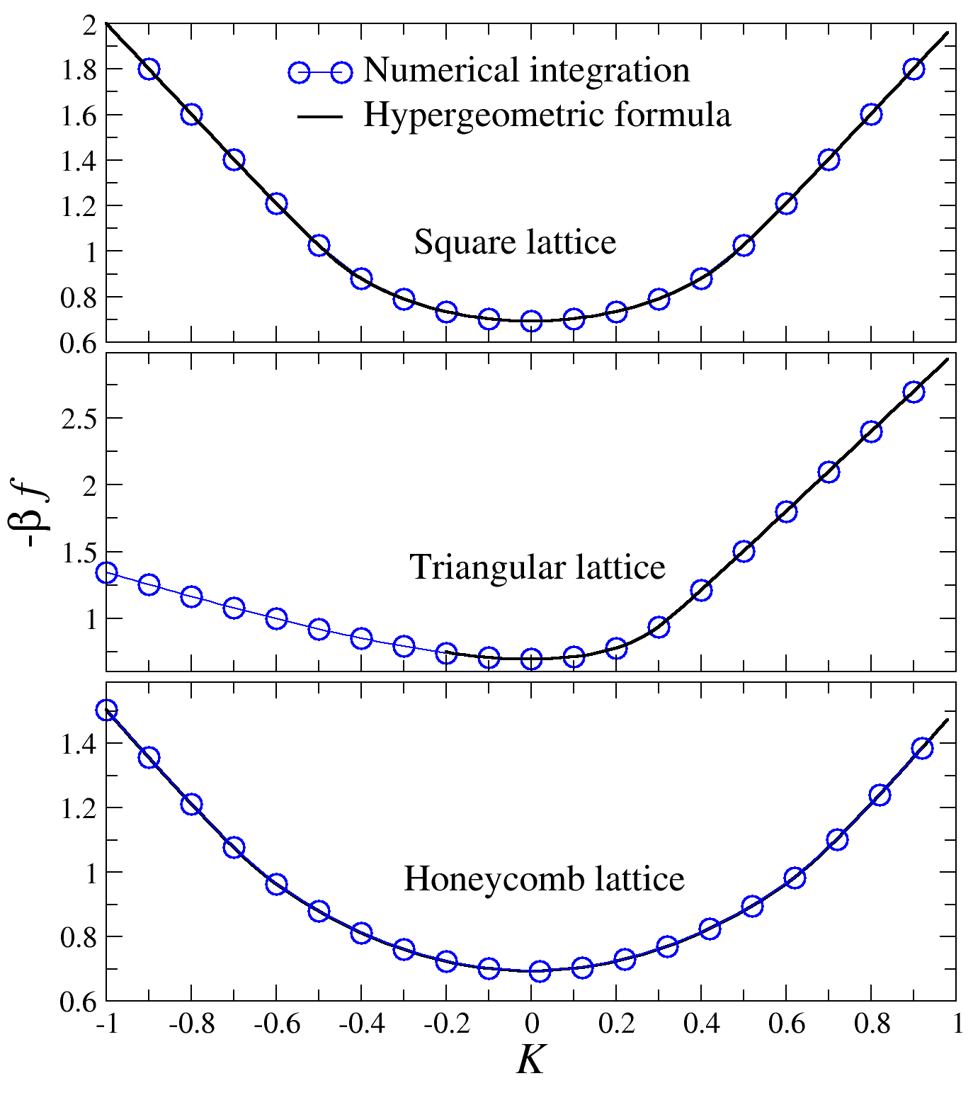
Figure 1: Comparison of $-\beta f=\log Z$ for the square, triangular and honeycomb lattices calculated via numerical integration and via the hypergeometric formulas.

Next, we obtain a connection with $L$-functions of elliptic curves, using (4) and (5) as illustrative examples. Let $K^{\prime}_{\square},\leavevmode\nobreak\ K^{\prime}_{\triangle}$ and $K^{\prime}_{\hexagon}$ be the temperatures corresponding to $k_{\square}=8$ and $k_{\triangle}=k_{\hexagon}=-4$. The choice $k_{\hexagon}=-4$ does not correspond to temperatures $K_{\hexagon}\in\mathbb{R}$. Since our goal is to show the connection with $L$-functions, we can obtain the required complex valued temperature $K_{\hexagon}\in\mathbb{C}$ via analytic continuation. Only one of several complex-valued temperatures is shown. For the square lattice, there are 2 real-valued temperatures corresponding to $k_{\square}=8$, only one of which we show here for illustration purposes. For the triangular lattice, the reduced temperature $K=\beta J$ is negative, which can be achieved for $\beta>0$ by choosing $J<0$. The values thus obtained are

$$K^{\prime}_{\square} =\frac{1}{2}\log\left(\sqrt{6}-\sqrt{2\sqrt{6}+5}+2\right)\approx 0.132\leavevmode\nobreak\ ,$$

$$K^{\prime}_{\triangle} =\frac{1}{4}\log\left(2\sqrt{3}-3\right)\approx-0.19\leavevmode\nobreak\ ,$$

$$K^{\prime}_{\hexagon} =\log\left(-\sqrt{\sqrt{3}-i\sqrt{2\sqrt{3}-3}-1}\right)\approx 2.77i\leavevmode\nobreak\ .$$

Substituting these and (4) and (5), into (26), we obtain a direct connection between the free energy and $L$-functions of elliptic curves:

$$-\beta f_{\square}(K^{\prime}_{\square}) =\frac{1}{2}\left(\log|\tfrac{1}{2}\sinh 2K_{\square}|+{24\over\pi^{2}}L(E_{24},2)\right)$$

$$\quad\quad+\log 2\leavevmode\nobreak\ ,$$

$$-\beta f_{\triangle}(K^{\prime}_{\triangle}) =\frac{1}{2}\left(\log|\tfrac{1}{2}\sinh 2K_{\triangle}|+{18\over\pi^{2}}L(E_{36},2)\right)$$

$$\quad\quad+\log 2\leavevmode\nobreak\ ,$$

$$-\beta f_{\hexagon}(K^{\prime}_{\hexagon}) =\frac{1}{4}\left(2\log|\sinh 2K_{\hexagon}|+{18\over\pi^{2}}L(E_{36},2)\right)$$

$$\quad\quad+\tfrac{1}{2}\log 2\leavevmode\nobreak\ .$$ (42)

We finally present our last result, unveiling a connection that might be even deeper. The positive critical temperatures are given by the singularities at $k_{\triangle}=k_{\hexagon}=8$ and $k_{\square}=4$. Using (6) and (7) in (26) and after simplification, we arrive at the critical free energy as Dirichlet $L$-functions $L(\chi,s)$ at $s=2$:

$$-\beta f_{\square}(K_{c}^{\square}) =\frac{1}{2}\log 2\leavevmode\nobreak\ +\leavevmode\nobreak\ {2\over\pi}\leavevmode\nobreak\ L(\chi_{-4},2)\leavevmode\nobreak\ ,$$

$$-\beta f_{\triangle}(K_{c}^{\triangle}) =\frac{1}{4}\log{4\over 3}+{15\sqrt{3}\over 8\pi}L(\chi_{-3},2)\leavevmode\nobreak\ ,$$

$$-\beta f_{\hexagon}(K_{c}^{\hexagon}) =\frac{1}{4}\log{12}+{15\sqrt{3}\over 16\pi}L(\chi_{-3},2)\leavevmode\nobreak\ .$$ (43)

Onsager’s critical free energy for the square lattice (see Eq. (121) in  onsager ) is usually written in terms of $G$, whereas in (43) we have highlighted instead the $L$-function.

Concluding remarks.

We have shown that Mahler measures can serve as a bridge connecting the Ising model with elliptic curves and $L$-functions. Eqs. (42) and (43) unveil unexpected relationships for the free energy. We emphasize that the latter is a physical quantity, while $L$-functions originate in number theory. They are fundamentally different — yet intriguingly related. As Poincaré once remarked poincare , the most valuable relationships are those that “reveal unsuspected relations between other facts, long since known, but wrongly believed to be unrelated to each other.” We hope that the findings presented above motivate others to further explore these and similar relationships.

Other advances include the identity (18) for Mahler measures, as well as the reformulation (26) in terms of Mahler measures, and similarly the Hypergeometric formulas (35) and (41) for the triangular and honeycomb lattices. In contrast, (29) has been known for more than a decade hucht2011 ; viswan2021 ; viswan2017-pre . It is noteworthy that Glasser and Onsager had derived a (different) hypergeometric formula in the 1970s that they never published viswan2021 .

Finally, we discuss the main limitations of this work and related open problems: (i) We have given only one example of a Hasse-Weil $L$-function for each of the three lattices, while the list in ref. rogers2010 yields several others. (ii) Only three lattices have been studied. Can we generalize to other planar lattices? The $Z$-invariant Ising model baxter ; yang2002 might be a promising candidate for further study. (iii) What of nonplanar lattices? Intriguingly, while spanning tree constants on planar lattices are related to $L$-functions $L(\cdot,s)$ evaluated at $s=2$, it is known guttmann2012 that on the simple cubic lattice the spanning tree constant can be expressed in terms of an $L$-function evaluated at $s=3$. Might the free energy of the critical Ising model on the simple cubic lattice similarly be given by an $L$-function at $s=3$ ?  Such fascinating questions are currently unanswerable because the 3D Ising model remains unsolved viswan-entropy ; perk1 ; perk2 ; perk3 ; perk4 . Exploring fresh ideas will be essential for advancing our understanding of these formidable challenges.

We thank J. H. H. Perk for discussions via e-mail over a period of several years. This work was supported by CNPq (Grant No. 302414/2022-3).

See pages 1 of sm.pdf See pages 2 of sm.pdf See pages 3 of sm.pdf See pages 4 of sm.pdf See pages 5 of sm.pdf See pages 6 of sm.pdf See pages 7 of sm.pdf

References

- (1) F. Brunault F and W. Zudilin, Many Variations of Mahler Measures: A Lasting Symphony (Cambridge University Press, Cambridge, 2020).
- (2) J. McKee and C. Smyth, Around the Unit Circle: Mahler Measure, Integer Matrices and Roots of Unity (Springer, Cham, 2021).
- (3) A. Zahabi, Toric quiver asymptotics and Mahler measure: BPS states, J. High Energ. Phys. 2019, 121 (2019).
- (4) J. Stienstra, Mahler measure variations, Eisenstein series and instanton expansions, in Mirror symmetry V, AMS/IP Studies in Advanced Mathematics, vol. 38, eds. N. Yui, S.-T. Yau and J. D. Lewis (International Press & American Mathematical Society, Providence, RI, 2006). arXiv:math/0502193
- (5) J. Bao, Y. H. He and A. Zahabi, A. Mahler Measure for a Quiver Symphony, Commun. Math. Phys. 394, 573 (2022).
- (6) G. Chesi, On the Mahler measure of matrix pencils, in 2013 American Control Conference (IEEE, Washington, 2013).
- (7) A. J. Guttmann and M. D Rogers, Spanning tree generating functions and Mahler measures, J. Phys. A: Math. Theor. 45, 494001 (2012).
- (8) G. M. Viswanathan Correspondence between spanning trees and the Ising model on a square lattice, Phys. Rev. E 95, 062138 (2017).
- (9) J. Stienstra, Mahler measure, Eisenstein series and dimers, in Mirror symmetry V, AMS/IP Studies in Advanced Mathematics, vol. 38, eds. N. Yui, S.-T. Yau and J. D. Lewis (International Press & American Mathematical Society, Providence, RI, 2006). arXiv:math/0502197
- (10) M. L. Glasser and F. Y. Wu, On the Entropy of Spanning Trees on a Large Triangular Lattice, Ramanujan J.10, 205–214 (2005).
- (11) M. L. Glasser and G. Lamb, A lattice spanning-tree entropy function J. Phys. A: Math. Gen. 38 L471 (2005).
- (12) R. Shrock and F. Y. Wu, Spanning trees on graphs and lattices in d dimensions J. Phys. A: Math. Gen. 33 3881 (2000).
- (13) M. L. Glasser, A note on a hyper-cubic Mahler measure and associated Bessel integral J. Phys. A: Math. Theor. 45, 494002 (2012).
- (14) D. W. Boyd, Speculations concerning the range of Mahler’s measure, Canad. Math. Bull., 24(4): 453 (1981).
- (15) D. W. Boyd, Mahler’s measure and special values of L-functions, Experiment. Math., 7(1), 37 (1998).
- (16) M. N. Lalín and Mathew D. Rogers, Functional equations for Mahler measures of genus-one curves 87–117 Algebra and Number Theory {1(1), 87 (2007).
- (17) F. R. Villegas, Modular Mahler Measures I, in: S. D. Ahlgren, G. E. Andrews, K. Ono (eds), Topics in Number Theory. Mathematics and Its Applications, vol 467 (Springer, Boston, 1999).
- (18) A. Bostan, S. Boukraa, S. Hassani, M. van Hoeij, J.-M. Maillard, J.-A. Weil and N. Zenine, The Ising model: from elliptic curves to modular forms and Calabi–Yau equations, Journal of Physics A: Mathematical and Theoretical, 44(4) 045204 (2011).
- (19) Y. M. Zinoviev, Ising Model and -Function, Theoretical and Mathematical Physics 126, 66 (2001).
- (20) S. Boukraa, S. Hassani, J.-M, Maillard and N. Zenine, From Holonomy of the Ising Model Form Factors to -Fold Integrals and the Theory of Elliptic Curves, SIGMA 3 099, 43 (2007).
- (21) G. M. Viswanathan, The double hypergeometric series for the partition function of the 2D anisotropic Ising model, J. Stat. Mech. bf 2021, 073104 (2021).
- (22) G. M. Viswanathan, M. A. G. Portillo, E. P. Raposo, M. G. E. da Luz, What Does It Take to Solve the 3D Ising Model? Minimal Necessary Conditions for a Valid Solution. Entropy 24, 1665. (2022).
- (23) R. J. Baxter, Exactly solved models in statistical mechanics (Academic Press, London,1989).
- (24) D. H. Lehmer, Factorization of certain cyclotomic functions, Ann. Math. 2. 34(3), 461 (1933).
- (25) K. Mahler, On some inequalities for polynomials in several variables, J. London Math. Soc., 37 341 (1962).
- (26) B. J. Ringeling, Mahler measures, modular forms and hypergeometric functions, Ph.D. thesis, Radboud University, Nijmegen (1993).
- (27) A. Mellit, Elliptic dilogarithms and parallel lines, arXiv:1207.4722 (2012).
- (28) Z. Tao, G. Xuejun and T. Wei, Mahler measures and -values of elliptic curves over real quadratic fields, arXiv:2209.14717 (2022).
- (29) Deninger C. Deninger, Deligne periods of mixed motives, -theory and the entropy of certain -actions. J. Amer. Math. Soc., 10(2):259–281, 1997.
- (30) M. Rogers, Hypergeometric Formulas for Lattice Sums and Mahler Measures, International Mathematics Research Notices, 2011(17), 4027 (2011). arXiv:0806.3590
- (31) A. Hucht, D. Grüneberg and F. M. Schmidt, Aspect-ratio dependence of thermodynamic Casimir forces, Phys. Rev. E 83, 051101 (2011).
- (32) L. Onsager, Crystal Statistics. I. A Two-Dimensional Model with an Order-Disorder Transition Phys. Rev. 65, 117 (1944).
- (33) R.M.F. Houtappel, Order-disorder in hexagonal lattices, Physica, 16(5), 425 (1950).
- (34) H. Poincaré Science and Method (T. Nelson, London, 1914).
- (35) H. Au-Yang and J. H. H. Perk, Correlation Functions and Susceptibility in the -Invariant Ising Model. In: M. Kashiwara and T. Miwa, T. (eds), MathPhys Odyssey 2001, Progress in Mathematical Physics 23 (Birkhäuser, Boston, 2002).
- (36) J. H. H. Perk, Comment on Zhang, D. Exact Solution for Three-Dimensional Ising Model. Symmetry 2021, 13, 1837, Symmetry 15(2), 374. (2023).
- (37) M. E. Fisher and J. H.H. Perk, Comments concerning the Ising model and two letters by N.H. March, Physics Letters A, 380(13) 1339 (2016).
- (38) J. H. H. Perk Comment on ’Mathematical structure of the three-dimensional (3D) Ising model’ Chinese Physics B 22(8), 080508 (2013).
- (39) J. H. H. Perk, Erroneous solution of three-dimensional (3D) simple orthorhombic Ising lattices Bulletin de la Société des Sciences et des Lettres de Łódż, Série: Recherches sur les Déformations 62(3), 45 (2013).