Suppressing Beam Squint Effect For Near-Field Wideband Communication Through Movable Antennas

Abstract

In this correspondence, we study deploying movable antenna (MA) array in a wideband multiple-input-single-output (MISO) communication system, where near-field (NF) channel model is considered. To alleviate beam squint effect, we propose to maximize the minimum analog beamforming gain across the entire wideband spectrum by appropriately adjusting MAs’ positions, which is a highly challenging task. By introducing a slack variable and adopting the cutting-the-edge smoothed-gradient-descent-ascent (SGDA) method, we develop algorithms to resolve the aforementioned challenge. Numerical results verify the effectiveness of our proposed algorithms and demonstrate the benefit of utilizing MA array to mitigate beam squint effect in NF wideband system.

I Introduction

Multiple-input-multiple-output (MIMO) technology is a critical technology to improve the spectral efficiency of the fifth-generation (5G) communication system and future wireless communications [1]. Very recently, a novel antenna architecture named movable antenna (MA) [2], also known as fluid antenna (FA) [3], has been proposed to further improve the beamforming capability. As opposed to the conventional fixed position antenna (FPA) array, which has its antenna elements fabricated on fixed positions, MAs can move freely within a specific area in programmable manner. This movability empowers antenna array with additional degree-of-freedom (DoF) and hence enhances its spatial multiplexing gain. MA array can be implemented by different techniques. For instance, the authors of [2] proposed a structure where MAs are connected with radio-frequency (RF)-chains and controlled by stepper motors. In [3], MA array was constructed using liquid metal technology.

Currently, a growing body of researches are exploring the potentials of MA array [4]-[7]. Specifically, the authors of [4] modeled the channel between a single-MA TX and a single-MA RX and theoretically proved that employment of MAs can improve signal-to-noise-ratio (SNR) performance. In [5], the authors considered deploying MA in a multi-user single-input-multiple-output (MU-SIMO) system and demonstrated that the use of MA can significantly lower the transmit power. The authors of [6] considered maximizing the minimal signal power of desired directions by jointly optimizing beamforming and MAs’ positions. As reported in [6], utilizing MAs can remarkably improve beamforming gain and suppress interference. In [7], the authors investigated a wideband single-input-single-output (SISO) system assisted by MAs and verified that implementing MAs can boost the achievable rate based on theoretical analysis and antenna position optimization.

Although exciting progresses have been made in the existing literature, e.g., [4]-[7], deploying MA array in wideband system has not yet been thoroughly investigated, except for [7]. Note one prominent challenge to employ MIMO in wideband system is the beam squint effect [8]-[11], i.e., analog beamforming gain degrades when subcarrier frequency deviates from the reference tone (usually the central carrier frequency). Besides, with the enlargement of antenna aperture, e.g., extremely-large (XL)-MIMO, and elevation of operating frequency, e.g., millimeter-wave (mmWave) and terahertz (THz), near-field (NF) propagation effect of electromagnetic waves will become apparent [10], [11]. However, most of the existing research, e.g., [4]-[7], are performed based on far-field (FF) channel model. Inspired by the above observations, we are motivated to investigate appropriate configuration method of MA array to effectively combat beam squint effect in NF wideband communication system. Our contributions are summarized in the following:

• To the best of authors’ knowledge, this is the first work studies beam squint effect in an NF wideband MA communication system.

• To alleviate beam squint effect, we propose a max-min criterion to configure the MAs’ positions, which maximizes the minimal analog beamforming gain over the entire wideband spectrum.

• To resolve the above challenging problem, we propose two algorithms based on appropriate transformation and smoothed-gradient-descent-ascent (SGDA) method [12]. Especially, the SGDA-based solution is highly efficient.

• Numerical results verify the effectiveness of our proposed algorithms and demonstrate the benefit of MA in alleviating beam squint effect in wideband system.

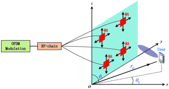
Fig. 1. Wideband MISO MA communication system.

II System Model and Problem Formulation

As shown in Fig. 1, we consider a wideband MISO communication system where a 2-D planar MA array with $M$ antennas residing in the $yoz$-plane serves a single-antenna user. Without loss of generality, we assume that the MA array has a square shape of size $A\times A$, locates its bottom left vertex at the origin of the coordinate system and arranges its neighboring edges parallel with the $y$- and $z$-axis, respectively. Denote $\mathcal{M}\triangleq\{1,\cdots,M\}$ as the set of MAs and $\bm{p}_{m}\triangleq[0,y_{m},z_{m}]^{\mathsf{T}},\;m\in\mathcal{M}$, as the position of the $m$-th MA. Since all MAs should maintain within the array surface area, the restriction $\bm{p}_{m}\in\mathcal{C}_{\mathrm{MA}}\triangleq\{(0,y,z)|y\in[0,A],\;z\in[0,A]\}$, for all $m\in\mathcal{M}$, should be satisfied with $\mathcal{C}_{\mathrm{MA}}$ indicating the feasible dwelling region of the MAs [4]-[7].

In this paper, we consider quasi-static NF channel model. In fact, wideband systems generally operate in frequency band, e.g., mmWave and THz, and hence have large Rayleigh distance. This implies that wireless channels should be captured via more accurate NF channel model [10], [11]. Especially, in typical NF propagation environment, line-of-sight (LoS) path significantly dominates the non-LoS paths and therefore the latter are negligible [10], [11]. Therefore, we adopt NF LoS channel model in the following discussion. As specified in Fig. 1, regarding the origin as the reference point, we define $\theta_{0}$, $\phi_{0}$, and $r_{0}$ as the azimuth angle, elevation angle, and distance of the user’s antenna, respectively.¹ Hence, the position of user’s antenna is given by $\bm{p}_{\mathrm{U}}=[r_{0}\mathsf{cos}\theta_{0}\mathsf{sin}\phi_{0},r_{0}\mathsf{sin}\theta_{0}\mathsf{sin}\phi_{0},r_{0}\mathsf{cos}\phi_{0}]^{\mathsf{T}}$. Furthermore, given the MAs’ positions $\{\bm{p}_{m}\}_{m=1}^{M}$, the normalized NF channel response vector at frequency $f$ reads

$$\bm{b}(\{\bm{p}_{m}\}_{m=1}^{M},\theta_{0},\phi_{0},r_{0},f)=[ e^{-j\frac{2\pi f}{c}\|\bm{p}_{\mathrm{U}}-\bm{p}_{1}\|_{2}},$$

$$\cdots,e^{-j\frac{2\pi f}{c}\|\bm{p}_{\mathrm{U}}-\bm{p}_{M}\|_{2}}]^{\mathsf{T}},$$ (1)

where $c$ is the speed of light. Based on Fresnel approximation [15], $\|\bm{p}_{\mathrm{U}}-\bm{p}_{m}\|_{2},\;m\in\mathcal{M}$, can be appropriately approximated as²

$$\|\bm{p}_{\mathrm{U}}-\bm{p}_{m}\|_{2}\approx r_{0}-y_{m}\mathsf{sin}\theta_{0}\mathsf{sin}\phi_{0}-z_{m}\mathsf{cos}\phi_{0}$$

$$+\frac{y_{m}^{2}+z_{m}^{2}-(y_{m}\mathsf{sin}\theta_{0}\mathsf{sin}\phi_{0}+z_{m}\mathsf{cos}\phi_{0})^{2}}{2r_{0}},\;m\in\mathcal{M}.$$ (2)

Analogous to conventional hybrid beamforming architecture, whose phase-shifter array determines the beam direction physically, MA system’s analog beam is conquered by adjustable MAs’ positions. To investigate the beam squint effect in wideband system, we consider the analog beamforming gain endowed by the MA array [8]-[11]. Specifically, denote the MA array’s beam steering vector as $\bm{w}(\{\bm{p}_{m}\}_{m=1}^{M},\theta_{0},\phi_{0},r_{0},f_{\mathrm{c}})$, which is similarly expressed in (1) with $f_{\mathrm{c}}$ being the central frequency. Then, the MAs’ analog beamforming gain is

$$\mathsf{g}(\{\bm{p}_{m}\}_{m\!=\!1}^{M},f_{\mathrm{c}},f)\!\!\triangleq\!\!|\bm{w}^{\mathsf{H}}(\{\bm{p}_{m}\}_{m\!=\!1}^{M},f_{\mathrm{c}})\bm{b}(\{\bm{p}_{m}\}_{m\!=\!1}^{M},f)|,$$ (3)

where $\bm{w}(\{\bm{p}_{m}\}_{m=1}^{M},f_{\mathrm{c}})$ and $\bm{b}(\{\bm{p}_{m}\}_{m=1}^{M},f)$ respectively represent $\bm{w}(\{\bm{p}_{m}\}_{m=1}^{M},\theta_{0},\phi_{0},r_{0},f_{\mathrm{c}})$ and $\bm{b}(\{\bm{p}_{m}\}_{m=1}^{M},\theta_{0},\phi_{0},r_{0},f)$ for simplicity.

As indicated by (3), analog beamforming gain depends on the subcarrier frequency $f$. For the wideband system, the carrier frequency $f$ varies over a wide spectrum and hence incurs severe fluctuating beamforming gain across subcarriers, which is the so-called beam squint effect. To provide more balanced communication rate among different subcarrier’s data stream [8], [9], we propose to maximize the minimum analog beamforming among the entire band. Specifically, denote the subcarrier frequencies as $\{f_{l}\}_{l=0}^{L}$ with $f_{0}<\cdots<f_{L}$. The configuration of MAs is formulated as the following problem

$$(\mathcal{P}1):\max_{\{\bm{t}_{m}\}_{m=1}^{M}} \min_{f\in\{f_{l}\}_{l=0}^{L}}\mathsf{g}^{2}(\{\bm{t}_{m}\}_{m=1}^{M},f_{\mathrm{c}},f)$$ (4)

$$\mathrm{s.t.}\; [0,\bm{t}_{m}^{\mathsf{T}}]^{\mathsf{T}}\in\mathcal{C}_{\mathrm{MA}},\;m\in\mathcal{M},$$ (4a)

$$\|\bm{t}_{m}-\bm{t}_{s}\|_{2}\geq D_{\mathrm{min}},\;m,s\!\in\!\mathcal{M},\;m\!\neq\!s,$$ (4b)

where $\bm{t}_{m}\triangleq[y_{m},z_{m}]^{\mathsf{T}},\;m\in\mathcal{M}$, constraint (4a) requires that all MAs should be in feasible region $\mathcal{C}_{\mathrm{MA}}$, and constraint (4b) ensures realistic spacing between MAs [4]-[7]. Obviously, $(\mathcal{P}1)$ is highly challenging due to its objective and nonconvex constraint (4b). In the following, we will develop algorithms to tackle $(\mathcal{P}1)$.

III Algorithm Design

In this section, via introducing a slack variable, we develop algorithm to solve the max-min problem $(\mathcal{P}1)$. Specifically, $(\mathcal{P}1)$ can be equivalently transformed into

$$(\mathcal{P}2): \max_{\{\bm{t}_{m}\}_{m=1}^{M},\kappa}\kappa$$ (5)

$$\mathrm{s.t.}\; \mathsf{g}^{2}(\{\bm{t}_{m}\}_{m=1}^{M},f_{\mathrm{c}},f_{l})\geq\kappa,\;l=0,\cdots,L,$$ (5a)

$$[0,\bm{t}_{m}^{\mathsf{T}}]^{\mathsf{T}}\in\mathcal{C}_{\mathrm{MA}},\;m\in\mathcal{M},$$ (5b)

$$\|\bm{t}_{m}-\bm{t}_{s}\|_{2}\geq D_{\mathrm{min}},\;m,s\in\mathcal{M},\;m\neq s.$$ (5c)

To obtain tractable solution, in the following, we adopt block coordinate descent (BCD) method to alternatively optimize one MA’s position at a time. Considering the optimization of the $m$-th MA’s position alone, $(\mathcal{P}2)$ reduces to

$$(\mathcal{P}3):\max_{\bm{t}_{m},\kappa}\; \kappa$$ (6)

$$\mathrm{s.t.}\; \mathsf{g}^{2}(\bm{t}_{m},f_{\mathrm{c}},f_{l})\geq\kappa,\;l=0,\cdots,L,$$ (6a)

$$[0,\bm{t}_{m}^{\mathsf{T}}]^{\mathsf{T}}\in\mathcal{C}_{\mathrm{MA}},$$ (6b)

$$\|\bm{t}_{m}-\bm{t}_{s}\|_{2}\geq D_{\mathrm{min}},\;s\in\mathcal{M},\;s\neq m.$$ (6c)

Note $(\mathcal{P}3)$ is still difficult due to the nonconvex constraints (6a) and (6c). To tackle this issue, we leverage majorization-minimization (MM) methodology [16] to construct concave lower-bounds for the left hand side of (6a) and (6c), respectively. Note in the following, we will use $\mathsf{h}(\bm{t}_{m},f_{l})\triangleq\mathsf{g}^{2}(\bm{t}_{m},f_{\mathrm{c}},f_{l}),\;m\in\mathcal{M},\;l=0,\cdots,L$, to simplify notations.

Firstly, to handle (6a), we examine the second-order Taylor expansion of the left hand side of (6a) and replace its Hessian matrix with a smaller one in the sense of Loewner ordering to obtain a tight globally lower bound surrogate. Specifically, the second-order Taylor expansion of $\mathsf{h}(\bm{t}_{m},f_{l})$ with respect to (w.r.t.) $\bm{t}_{m}$ at the point $\bm{t}_{m}^{(n)}$ reads

$$\mathsf{h}(\bm{t}_{m},f_{l})\approx\mathsf{h}(\bm{t}_{m}^{(n)},f_{l})+\nabla_{\bm{t}_{m}}^{\mathsf{T}}(\mathsf{h}(\bm{t}_{m},f_{l}))|_{\bm{t}_{m}=\bm{t}_{m}^{(n)}}(\bm{t}_{m}-\bm{t}_{m}^{(n)})$$

$$+\frac{1}{2}(\bm{t}_{m}-\bm{t}_{m}^{(n)})^{\mathsf{T}}\nabla_{\bm{t}_{m}}^{2}(\mathsf{h}(\bm{t}_{m},f_{l}))|_{\bm{t}_{m}=\bm{t}_{m}^{(n)}}(\bm{t}_{m}-\bm{t}_{m}^{(n)}),$$ (7)

where $\nabla_{\bm{t}_{m}}(\mathsf{h}(\bm{t}_{m},f_{l}))$ and $\nabla_{\bm{t}_{m}}^{2}(\mathsf{h}(\bm{t}_{m},f_{l}))$ are derived in Appendix A. Furthermore, it can be observed that the Hessian matrix $\nabla_{\bm{t}_{m}}^{2}(\mathsf{h}(\bm{t}_{m},f_{l}))$ can be lower-bounded by $\min\{\lambda_{\mathrm{min}}(\nabla_{\bm{t}_{m}}^{2}(\mathsf{h}(\bm{t}_{m},f_{l}))),0\}\mathbf{I}_{2}$, where $\lambda_{\mathrm{min}}(\mathbf{X})$ and $\mathbf{I}_{2}$ represent the minimal eigenvalue of matrix $\mathbf{X}$ and the identity matrix of size $2\times 2$, respectively. Therefore, we can obtain a global concave lower-bound of $\mathsf{h}(\bm{t}_{m},f_{l})$ by substituting $\min\{\lambda_{\mathrm{min}}(\nabla_{\bm{t}_{m}}^{2}(\mathsf{h}(\bm{t}_{m},f_{l}))),0\}\mathbf{I}_{2}$ into (7).

Next, we convexify the constraint (6c), which is much easier since the left hand side of (6c) is convex w.r.t. $\bm{t}_{m}$. By directly utilizing the following first-order Taylor expansion

$$\|\bm{t}_{m}-\bm{t}_{s}\|_{2}\geq\frac{(\bm{t}_{m}^{(n)}-\bm{t}_{s})^{\mathsf{T}}}{\|\bm{t}_{m}^{(n)}-\bm{t}_{s}\|_{2}}(\bm{t}_{m}-\bm{t}_{s}),\;s\in\mathcal{M},\;s\neq m,$$ (8)

a concave lower-bound of $\|\bm{t}_{m}-\bm{t}_{s}\|_{2}$ has been obtained.

After surrogating the left hand side of (6a) and (6c) by the two lower-bounds developed above, we acquire the following convex optimization problem

$$(\mathcal{P}4): \max_{\bm{t}_{m},\kappa}\;\kappa$$ (9)

$$\mathrm{s.t.}\; \mathsf{h}(\bm{t}_{m},f_{l}|\bm{t}_{m}^{(n)})\geq\kappa,\;l=0,\cdots,L,$$ (9a)

$$[0,\bm{t}_{m}^{\mathsf{T}}]^{\mathsf{T}}\in\mathcal{C}_{\mathrm{MA}},$$ (9b)

$$\frac{(\bm{t}_{m}^{(n)}-\bm{t}_{s})^{\mathsf{T}}}{\|\bm{t}_{m}^{(n)}-\bm{t}_{s}\|_{2}}(\bm{t}_{m}-\bm{t}_{s})\geq D_{\mathrm{min}},\;s\in\mathcal{M},\;s\neq m,$$ (9c)

which can be solved by numerical solvers, e.g., CVX, where

$$\mathsf{h}(\bm{t}_{m},f_{l}|\bm{t}_{m}^{(n)})\!\!\triangleq\!\!\mathsf{h}(\bm{t}_{m}^{(n)},f_{l})\!\!+\!\!\nabla_{\bm{t}_{m}}^{\mathsf{T}}(\mathsf{h}(\bm{t}_{m},f_{l}))|_{\bm{t}_{m}=\bm{t}_{m}^{(n)}}(\bm{t}_{m}\!\!-\!\!\bm{t}_{m}^{(n)})$$

$$\!+\!\frac{\min\big{\{}\lambda_{\mathrm{min}}\big{(}\nabla_{\bm{t}_{m}}^{2}(\mathsf{h}(\bm{t}_{m},f_{l}))|_{\bm{t}_{m}=\bm{t}_{m}^{(n)}}\big{)},0\big{\}}}{2}\|\bm{t}_{m}\!\!-\!\!\bm{t}_{m}^{(n)}\|_{2}^{2}.$$ (10)

The proposed solution to $(\mathcal{P}1)$ by introducing a slack variable is summarized in Algorithm 1.

1:  Initialize feasible $\{\bm{t}_{m}^{(0)}\}_{m=1}^{M}$ and $n=0$;

2:  repeat

3:     for $m=1$ to $M$ do

4:        update $(\bm{t}_{m}^{(n+1)},\kappa^{(n+\frac{m}{M})})$ by solving $(\mathcal{P}4)$;

5:     end for

6:     $n:=n+1$;

7:  until convergence

Algorithm 1 Solving $(\mathcal{P}1)$ based on slack variable

IV SGDA-Based Efficient Solution

Note one potential defect of Alg. 1 proposed above lies in its complexity. In fact, wideband system generally has a great number, e.g., up to hundreds or thousands, of subcarriers. This makes $(\mathcal{P}4)$ a second-order cone programming (SOCP) problem with a large number of constraints and hence significantly inflates its computational complexity. In this section, we proceed to develop an efficient algorithm based on SGDA method.

We still exploit BCD framework to optimize the antenna positions. Before invoking SGDA algorithm, we convexify constraint (4b) by (8), and regard $f$ as a continuous parameter, i.e., $f\in[f_{0},f_{L}]$.³ Hence, the optimization for the $m$-th MA’s position can be casted as

$$(\mathcal{P}5): \max_{\bm{t}_{m}}\min_{f\in[f_{0},f_{L}]}\mathsf{h}(\bm{t}_{m},f)$$ (11)

$$\mathrm{s.t.}\; [0,\bm{t}_{m}^{\mathsf{T}}]^{\mathsf{T}}\in\mathcal{C}_{\mathrm{MA}},$$ (11a)

$$\frac{(\bm{t}_{m}^{(n)}\!-\!\bm{t}_{s})^{\mathsf{T}}}{\|\bm{t}_{m}^{(n)}\!-\!\bm{t}_{s}\|_{2}}(\bm{t}_{m}\!-\!\bm{t}_{s})\geq D_{\mathrm{min}},\;s\in\mathcal{M},\;s\neq m.$$ (11b)

Next, we adopt SGDA method to tackle $(\mathcal{P}5)$. Note GDA methodology solves max-min problem via alternatively conducting gradient ascent (GA) and gradient descent (GD) updates towards maximization and minimization, respectively. Besides, by introducing additional smoothing terms, SGDA further improves the convergence of the standard GDA method [12]. Specifically, according to SGDA method [12], by introducing auxiliary variables $\{\bm{\alpha}_{m}\}_{m=1}^{M}$ and defining a function

$$\mathsf{k}(\bm{t}_{m},\bm{\alpha}_{m};f)\triangleq\mathsf{h}(\bm{t}_{m},f)+\frac{p_{\mathrm{S}}}{2}\|\bm{t}_{m}-\bm{\alpha}_{m}\|_{2}^{2},$$ (12)

where $p_{\mathrm{S}}>0$ is a pre-defined constant, we alternatively update $\bm{t}_{m}$ in a GA manner and $f$ and $\bm{\alpha}_{m}$ in GD manners in each iteration. Denote $(\bm{t}_{m}^{(n)},f^{(n)},\bm{\alpha}_{m}^{(n)})$ as the solution iterate updated in the $n$-th iteration. The detailed updates will be elaborated in the following discussions.

A. Update of $\bm{t}_{m}$

The variable $\bm{t}_{m}$ is updated in a GA manner, given as follows

$$\bm{t}_{m}^{(n+1)}:=\bm{t}_{m}^{(n)}+\eta_{\bm{t}_{m}}^{(n)}\nabla_{\bm{t}_{m}}(\mathsf{k}(\bm{t}_{m},\bm{\alpha}_{m}^{(n)};f^{(n)}))|_{\bm{t}_{m}=\bm{t}_{m}^{(n)}},$$ (13)

where $\eta_{\bm{t}_{m}}^{(n)}$ is the updating step size and can be set as a constant [12], and $\nabla_{\bm{t}_{m}}(\mathsf{k}(\bm{t}_{m},\bm{\alpha}_{m};f))$ is

$$\nabla_{\bm{t}_{m}}(\mathsf{k}(\bm{t}_{m},\bm{\alpha}_{m};f))=\nabla_{\bm{t}_{m}}(\mathsf{h}(\bm{t}_{m},f))+p_{\mathrm{S}}(\bm{t}_{m}-\bm{\alpha}_{m}),$$ (14)

where $\nabla_{\bm{t}_{m}}(\mathsf{h}(\bm{t}_{m},f))$ is given in Appendix A.

Note that the newly obtained $\bm{t}_{m}^{(n+1)}$ may not satisfy (11a) or (11b). If so, $\bm{t}_{m}^{(n+1)}$ must be projected onto the convex domain constituted by (11a) and (11b), which is meant to solve the following optimization

$$(\mathcal{P}6): \min_{\bm{x}\in\mathbb{R}^{2}}\;\frac{1}{2}\|\bm{x}-\bm{t}_{m}^{(n+1)}\|_{2}^{2}$$ (15)

$$\mathrm{s.t.}\; [0,\bm{x}^{\mathsf{T}}]^{\mathsf{T}}\in\mathcal{C}_{\mathrm{MA}},$$ (15a)

$$\frac{(\bm{t}_{m}^{(n)}\!-\!\bm{t}_{s})^{\mathsf{T}}}{\|\bm{t}_{m}^{(n)}\!-\!\bm{t}_{s}\|_{2}}(\bm{x}\!-\!\bm{t}_{s})\geq D_{\mathrm{min}},\;s\in\mathcal{M},\;s\neq m.$$ (15b)

Problem $(\mathcal{P}6)$ is convex which can be numerically solved.

B. Update of $f$

The variable $f$ is updated in a GD manner, i.e.,

$$f^{(n+1)}:=f^{(n)}-\eta_{f}^{(n)}\nabla_{f}(\mathsf{k}(\bm{t}_{m}^{(n+1)},\bm{\alpha}_{m}^{(n)};f))|_{f=f^{(n)}},$$ (16)

where $\eta_{f}^{(n)}$ is the updating step size and can also be set as a constant [12]. The calculation of $\nabla_{f}(\mathsf{k}(\bm{t}_{m},\bm{\alpha}_{m};f))$ is relegated to Appendix B.

Obviously, there exists a possibility that $f^{(n+1)}$ falls out of the feasible domain $[f_{0},f_{L}]$. When this occurs, we should project $f^{(n+1)}$ onto $[f_{0},f_{L}]$, that is:

• If $f^{(n+1)}<f_{0}$, $f^{(n+1)}=f_{0}$,

• or if $f^{(n+1)}>f_{L}$, $f^{(n+1)}=f_{L}$.

C. Update of $\bm{\alpha}_{m}$

The variable $\bm{\alpha}_{m}$ is updated as follows [12]

$$\bm{\alpha}_{m}^{(n+1)}:=\bm{\alpha}_{m}^{(n)}+\eta_{\bm{\alpha}_{m}}^{(n)}(\bm{t}_{m}^{(n+1)}-\bm{\alpha}_{m}^{(n)}),$$ (17)

where $\eta_{\bm{\alpha}_{m}}^{(n)}\in(0,1]$ is a constant.

The proposed SGDA-based algorithm to tackle $(\mathcal{P}1)$ is summarized in Algorithm 2.

1:  Initialize feasible $\{\bm{t}_{m}^{(0)}\}_{m=1}^{M}$ and $i=0$;

2:  repeat

3:     for $m=1$ to $M$ do

4:        set $\bm{t}_{m}^{(i,0)}:=\bm{t}_{m}^{(i)}$, $\bm{\alpha}_{m}^{(i,0)}:=\bm{t}_{m}^{(i,0)}$ and $n=0$;

5:        randomly generate $f^{(i,0)}\in[f_{0},f_{L}]$;

6:        repeat

7:           update $\bm{t}_{m}^{(i,n+1)}$ by (13);

8:           project $\bm{t}_{m}^{(i,n+1)}$ by solving $(\mathcal{P}6)$ (if needed);

9:           update $f^{(i,n+1)}$ by (16);

110:           project $f^{(i,n+1)}$ by $f^{(i,n+1)}=f_{0}$

or $f^{(i,n+1)}=f_{L}$ (if needed);

11:           update $\bm{\alpha}_{m}^{(i,n+1)}$ by (17);

12:           $n:=n+1$;

13:        until convergence

14:        set $\bm{t}_{m}^{(i+1)}:=\bm{t}_{m}^{(i,\infty)}$ and $\bm{\alpha}_{m}^{(i+1)}:=\bm{\alpha}_{m}^{(i,\infty)}$;

15:     end for

16:     $i:=i+1$;

17:  until convergence

Algorithm 2 Solving $(\mathcal{P}1)$ based on SGDA

V Simulation Results

In this section, numerical results are provided to demonstrate the effectiveness of our proposed algorithms and the benefit of deploying MA array in wideband communication system. Unless otherwise specified, $L=256$, $f_{0}=30\mathrm{GHz}$, $f_{L}=50\mathrm{GHz}$, $f_{\mathrm{c}}=\frac{f_{0}+f_{L}}{2}=40\mathrm{GHz}$, $f_{l}=f_{0}+\frac{l}{L}(f_{L}-f_{0}),\;l=0,\cdots,L$, $A=\frac{2\sqrt{M}c}{f_{0}}$, $D_{\mathrm{min}}=\frac{c}{2f_{0}}$, $\theta_{0}=\frac{\pi}{6}$, $\phi_{0}=\frac{\pi}{4}$, $r_{0}=10\mathrm{m}$, $p_{\mathrm{S}}=2$, $\eta_{\bm{\alpha}_{m}}=0.5,\;m\in\mathcal{M}$.

Fig. 2 illustrates the convergence behaviours of Alg. 1 & 2. As suggested by Fig. 2, by utilizing Alg. 1, the objective value of $(\mathcal{P}1)$ monotonically increases and converges in ten iterations. At the same time, SGDA-based Alg. 2 exhibits fast improvement with slight oscillations. Interestingly, besides its lower complexity, Alg. 2 yields a superior converged objective value over Alg. 1.

Fig. 3 plots the array gain (defined in (3)) across different subcarriers. As reflected by Fig. 3, via appropriately configuring the antennas’ positions, MA can remarkably mitigate the beam squint effect compared to the conventional FPA counterpart. Note that the analog beamforming gain yielded by Alg. 2 outperforms Alg. 1 over the entire wide frequency band.

Lastly, to examine the complexity of our proposed algorithms, we compare both average MATLAB run-time per iteration in Fig. 4. As reflected by Fig. 4, the run-time of Alg. 1 increases intensively when the number of subcarriers $L$ grows. In contrast, the run-time per iteration of Alg. 2 is nearly insensitive to $L$ and maintains a much lower level than that of Alg. 1.

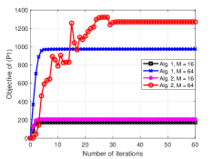
Fig. 2. Convergence behaviours of Alg. 1 & 2.

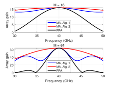
Fig. 3. Array gain across considered frequency band.

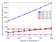
Fig. 4. Comparison of running time between Alg. 1 & 2.

VI Conclusion

In this paper, a wideband MISO communication system aided by MA array under NF channel model is considered. To overcome beam squint effect, a minimal array gain maximization criterion is proposed to configure MAs’ positions. We successfully develop algorithms based on introducing a slack variable and SGDA method. The SGDA-based algorithm has much lower complexity and is especially suitable to systems with large bandwidth. Simulation results verify that beam squint effect can be significantly mitigated by MA array deployment.

A. Calculation of $\nabla_{\bm{t}_{m}}(\mathsf{h}(\bm{t}_{m},f_{l}))$ and $\nabla_{\bm{t}_{m}}^{2}(\mathsf{h}(\bm{t}_{m},f_{l}))$

Define $C_{m,l}\triangleq\sum_{n=1,n\neq m}^{M}e^{j\frac{2\pi(f_{\mathrm{c}}-f_{l})}{c}\mathsf{a}(\bm{t}_{n})},\;m\in\mathcal{M},\;l=0,\cdots,L$, where $\mathsf{a}(\bm{t}_{m})\triangleq r_{0}-y_{m}\mathsf{sin}\theta_{0}\mathsf{sin}\phi_{0}-z_{m}\mathsf{cos}\phi_{0}+\frac{y_{m}^{2}+z_{m}^{2}-(y_{m}\mathsf{sin}\theta_{0}\mathsf{sin}\phi_{0}+z_{m}\mathsf{cos}\phi_{0})^{2}}{2r_{0}},\;m\in\mathcal{M}$. Then, after some manipulations, $\mathsf{h}(\bm{t}_{m},f_{l})$ can be expressed as

$$\mathsf{h}(\bm{t}_{m},f_{l}) =2|C_{m,l}|\mathsf{cos}\bigg{(}\frac{2\pi(f_{\mathrm{c}}-f_{l})}{c}\mathsf{a}(\bm{t}_{m})-\angle(C_{m,l})\bigg{)}$$

$$+|C_{m,l}|^{2}+1,\;m\in\mathcal{M},\;l=0,\cdots,L,$$ (18)

where $\angle(x)$ picks up the phase of input complex scalar $x$.

The gradient $\nabla_{\bm{t}_{m}}(\mathsf{h}(\bm{t}_{m},f_{l}))$ is given by

$$\nabla_{\bm{t}_{m}}(\mathsf{h}(\bm{t}_{m},f_{l}))=\bigg{[}\frac{\partial\mathsf{h}(\bm{t}_{m},f_{l})}{\partial y_{m}},\frac{\partial\mathsf{h}(\bm{t}_{m},f_{l})}{\partial z_{m}}\bigg{]}^{\mathsf{T}},$$ (19)

where

$$\frac{\partial\mathsf{h}(\bm{t}_{m},f_{l})}{\partial y_{m}}=-2|C_{m,l}|\frac{2\pi(f_{\mathrm{c}}-f_{l})}{c}\frac{\partial\mathsf{a}(\bm{t}_{m})}{\partial y_{m}}$$

$$\times\mathsf{sin}\bigg{(}\frac{2\pi(f_{\mathrm{c}}-f_{l})}{c}\mathsf{a}(\bm{t}_{m})-\angle(C_{m,l})\bigg{)},$$ (20)

$$\frac{\partial\mathsf{a}(\bm{t}_{m})}{\partial y_{m}}=\frac{y_{m}-(y_{m}\mathsf{sin}\theta_{0}\mathsf{sin}\phi_{0}+z_{m}\mathsf{cos}\phi_{0})\mathsf{sin}\theta_{0}\mathsf{sin}\phi_{0}}{r_{0}}$$

$$-\mathsf{sin}\theta_{0}\mathsf{sin}\phi_{0},$$ (21)

$$\frac{\partial\mathsf{h}(\bm{t}_{m},f_{l})}{\partial z_{m}}=-2|C_{m,l}|\frac{2\pi(f_{\mathrm{c}}-f_{l})}{c}\frac{\partial\mathsf{a}(\bm{t}_{m})}{\partial z_{m}}$$

$$\times\mathsf{sin}\bigg{(}\frac{2\pi(f_{\mathrm{c}}-f_{l})}{c}\mathsf{a}(\bm{t}_{m})-\angle(C_{m,l})\bigg{)},$$ (22)

$$\frac{\partial\mathsf{a}(\bm{t}_{m})}{\partial z_{m}}\!\!=\!\!\frac{z_{m}\!\!-\!\!(y_{m}\mathsf{sin}\theta_{0}\mathsf{sin}\phi_{0}\!\!+\!\!z_{m}\mathsf{cos}\phi_{0})\mathsf{cos}\phi_{0}}{r_{0}}\!-\!\mathsf{cos}\phi_{0}.$$ (23)

The Hessian matrix $\nabla_{\bm{t}_{m}}^{2}(\mathsf{h}(\bm{t}_{m},f_{l}))$ is given as follows

$$\nabla_{\bm{t}_{m}}^{2}(\mathsf{h}(\bm{t}_{m},f_{l}))=\begin{bmatrix}\frac{\partial^{2}\mathsf{h}(\bm{t}_{m},f_{l})}{\partial y_{m}^{2}}&\frac{\partial^{2}\mathsf{h}(\bm{t}_{m},f_{l})}{\partial y_{m}\partial z_{m}}\\ \frac{\partial^{2}\mathsf{h}(\bm{t}_{m},f_{l})}{\partial z_{m}\partial y_{m}}&\frac{\partial^{2}\mathsf{h}(\bm{t}_{m},f_{l})}{\partial z_{m}^{2}}\\ \end{bmatrix},$$ (24)

where

$$\frac{\partial^{2}\mathsf{h}(\bm{t}_{m},f_{l})}{\partial y_{m}^{2}}=-2|C_{m,l}|\frac{2\pi(f_{\mathrm{c}}-f_{l})}{c}\frac{1-(\mathsf{sin}\theta_{0}\mathsf{sin}\phi_{0})^{2}}{r_{0}}$$

$$\!\times\!\mathsf{sin}\bigg{(}\frac{2\pi(f_{\mathrm{c}}\!-\!f_{l})}{c}\mathsf{a}(\bm{t}_{m})\!-\!\angle(C_{m,l})\bigg{)}\!-\!2|C_{m,l}|\bigg{(}\frac{2\pi(f_{\mathrm{c}}\!-\!f_{l})}{c}\bigg{)}^{2}$$

$$\!\times\!\bigg{(}\frac{\partial\mathsf{a}(\bm{t}_{m})}{\partial y_{m}}\bigg{)}^{2}\mathsf{cos}\bigg{(}\frac{2\pi(f_{\mathrm{c}}\!-\!f_{l})}{c}\mathsf{a}(\bm{t}_{m})\!-\!\angle(C_{m,l})\bigg{)},$$ (25)

$$\frac{\partial^{2}\mathsf{h}(\bm{t}_{m},f_{l})}{\partial y_{m}\partial z_{m}}=-2|C_{m,l}|\frac{2\pi(f_{\mathrm{c}}-f_{l})}{c}\frac{-\mathsf{sin}\theta_{0}\mathsf{sin}\phi_{0}\mathsf{cos}\phi_{0}}{r_{0}}$$

$$\!\times\!\mathsf{sin}\bigg{(}\frac{2\pi(f_{\mathrm{c}}\!-\!f_{l})}{c}\mathsf{a}(\bm{t}_{m})\!-\!\angle(C_{m,l})\bigg{)}\!-\!2|C_{m,l}|\bigg{(}\frac{2\pi(f_{\mathrm{c}}\!-\!f_{l})}{c}\bigg{)}^{2}$$

$$\!\times\!\frac{\partial\mathsf{a}(\bm{t}_{m})}{\partial y_{m}}\frac{\partial\mathsf{a}(\bm{t}_{m})}{\partial z_{m}}\mathsf{cos}\bigg{(}\frac{2\pi(f_{\mathrm{c}}\!-\!f_{l})}{c}\mathsf{a}(\bm{t}_{m})\!-\!\angle(C_{m,l})\bigg{)},$$ (26)

$$\frac{\partial^{2}\mathsf{h}(\bm{t}_{m},f_{l})}{\partial z_{m}\partial y_{m}}=\frac{\partial^{2}\mathsf{h}(\bm{t}_{m},f_{l})}{\partial y_{m}\partial z_{m}},$$ (27)

$$\frac{\partial^{2}\mathsf{h}(\bm{t}_{m},f_{l})}{\partial z_{m}^{2}}=-2|C_{m,l}|\frac{2\pi(f_{\mathrm{c}}-f_{l})}{c}\frac{1-\mathsf{cos}^{2}\phi_{0}}{r_{0}}$$

$$\!\times\!\mathsf{sin}\bigg{(}\frac{2\pi(f_{\mathrm{c}}\!-\!f_{l})}{c}\mathsf{a}(\bm{t}_{m})\!-\!\angle(C_{m,l})\bigg{)}\!-\!2|C_{m,l}|\bigg{(}\frac{2\pi(f_{\mathrm{c}}\!-\!f_{l})}{c}\bigg{)}^{2}$$

$$\!\times\!\bigg{(}\frac{\partial\mathsf{a}(\bm{t}_{m})}{\partial z_{m}}\bigg{)}^{2}\mathsf{cos}\bigg{(}\frac{2\pi(f_{\mathrm{c}}\!-\!f_{l})}{c}\mathsf{a}(\bm{t}_{m})\!-\!\angle(C_{m,l})\bigg{)}.$$ (28)

B. Calculation of $\nabla_{f}(\mathsf{k}(\bm{t}_{m},\bm{\alpha}_{m};f))$

The gradient $\nabla_{f}(\mathsf{k}(\bm{t}_{m},\bm{\alpha}_{m};f))$ can be written as

$$\nabla_{f}(\mathsf{k}(\bm{t}_{m},\bm{\alpha}_{m};f))\!\! =\!\!\bm{w}^{\mathsf{H}}\frac{\partial\bm{b}(f)}{\partial f}\bm{b}^{\mathsf{H}}(f)\bm{w}\!\!+\!\!\bm{w}^{\mathsf{H}}\bm{b}(f)\bigg{(}\frac{\partial\bm{b}(f)}{\partial f}\bigg{)}^{\mathsf{H}}\bm{w}$$

$$=2\mathsf{Re}\bigg{\{}\bm{w}^{\mathsf{H}}\frac{\partial\bm{b}(f)}{\partial f}\bm{b}^{\mathsf{H}}(f)\bm{w}\bigg{\}},$$ (29)

where $\bm{w}$ and $\bm{b}(f)$ are short for $\bm{w}(\{\bm{t}_{m}\}_{m=1}^{M},f_{\mathrm{c}})$ and $\bm{b}(\{\bm{t}_{m}\}_{m=1}^{M},f)$, respectively. Besides, the $m$-th element of $\frac{\partial\bm{b}(f)}{\partial f}$ is given by

$$\bigg{[}\frac{\partial\bm{b}(f)}{\partial f}\bigg{]}_{m}=-j\frac{2\pi}{c}\mathsf{a}(\bm{t}_{m})[\bm{b}(f)]_{m},\;m\in\mathcal{M}.$$ (30)

References

• [1] E. G. Larsson, O. Edfors, F. Tufvesson, and T. L. Marzetta, “Massive MIMO for next generation wireless systems,” IEEE Commun. Mag., vol. 52, no. 2, pp. 186–195, Feb. 2014.
• [2] L. Zhu, W. Ma, and R. Zhang, “Movable antennas for wireless communication: Opportunities and challenges,” IEEE Commun. Mag., vol. 62, no. 6, pp. 114–120, Jun. 2024.
• [3] K.-K. Wong, A. Shojaeifard, K.-F. Tong, and Y. Zhang, “Fluid antenna systems,” IEEE Trans. Wireless Commun., vol. 20, no. 3, pp. 1950–1962, Mar. 2021.
• [4] L. Zhu, W. Ma, and R. Zhang, “Modeling and performance analysis for movable antenna enabled wireless communications,” IEEE Trans. Wireless Commun., vol. 23, no. 6, pp. 6234–6250, Jun. 2024.
• [5] L. Zhu, W. Ma, B. Ning, and R. Zhang, “Movable-antenna enhanced multiuser communication via antenna position optimization,” IEEE Trans. Wireless Commun., vol. 23, no. 7, pp. 7214–7229, Jul. 2024.
• [6] W. Ma, L. Zhu, and R. Zhang, “Multi-beam forming with movable-antenna array,” IEEE Commun. Lett., vol. 28, no. 3, pp. 697–701, Mar. 2024.
• [7] L. Zhu, W. Ma, Z. Xiao, and R. Zhang, “Performance analysis and optimization for movable antenna aided wideband communications,” arXiv preprint arXiv:2401.08974, 2024.
• [8] R. W. Heath Jr., N. G.-Prelcic, S. Rangan, W. Roh, and A. M. Sayeed, “An overview of signal processing techniques for millimeter wave MIMO systems,” IEEE J. Sel. Topics Signal Process., vol. 10, no. 3, pp. 436–453, Apr. 2016.
• [9] F. Gao, B. Wang, C. Xing, J. An, and G. Y. Li, “Wideband beamforming for hybrid massive MIMO terahertz communications,” IEEE J. Sel. Areas Commun., vol. 39, no. 6, pp. 1725–1740, Jun. 2021.
• [10] M. Cui, L. Dai, Z. Wang, S. Zhou, and N. Ge, “Near-field rainbow: Wideband beam training for XL-MIMO,” IEEE Trans. Wireless Commun., vol. 22, no. 6, pp. 3899–3912, Jun. 2023.
• [11] H. Luo, F. Gao, W. Yuan, and S. Zhang, “Beam squint assisted user localization in near-field integrated sensing and communications systems,” IEEE Trans. Wireless Commun., vol. 23, no. 5, pp. 4504–4517, May 2024.
• [12] J. Zhang, P. Xiao, R. Sun, and Z.-Q. Luo, “A single-loop smoothed gradient descent-ascent algorithm for nonconvex-concave min-max problems,” in Proc. 34th Conference on Neural Information Processing Systems (NeurIPS 2020), Vancouver, Canada, 2020.
• [13] W. Ma, L. Zhu, and R. Zhang, “Compressed sensing based channel estimation for movable antenna communications,” IEEE Commun. Lett., vol. 27, no. 10, pp. 2747–2751, Oct. 2023.
• [14] Z. Xiao, S. Cao, L. Zhu, Y. Liu, X.-G. Xia, and R. Zhang, “Channel estimation for movable antenna communication systems: A framework based on compressed sensing,” arXiv preprint arXiv:2312.06969, 2023.
• [15] K. T. Selvan and R. Janaswamy, “Fraunhofer and Fresnel distances: Unified derivation for aperture antennas,” IEEE Antennas Propag. Mag., vol. 59, no. 4, pp. 12–15, Aug. 2017.
• [16] Y. Sun, P. Babu, and D. P. Palomar, “Majorization-minimization algorithms in signal processing, communications, and machine learning,” IEEE Trans. Signal Process., vol. 65, no. 3, pp. 794–816, Feb. 2017.