Small-Gain Theorem Based Distributed Prescribed-Time Convex Optimization For Networked Euler-Lagrange Systems

Abstract

In this paper, we address the distributed prescribed-time convex optimization (DPTCO) for a class of networked Euler-Lagrange systems under undirected connected graphs. By utilizing position-dependent measured gradient value of local objective function and local information interactions among neighboring agents, a set of auxiliary systems is constructed to cooperatively seek the optimal solution. The DPTCO problem is then converted to the prescribed-time stabilization problem of an interconnected error system. A prescribed-time small-gain criterion is proposed to characterize prescribed-time stabilization of the system, offering a novel approach that enhances the effectiveness beyond existing asymptotic or finite-time stabilization of an interconnected system. Under the criterion and auxiliary systems, innovative adaptive prescribed-time local tracking controllers are designed for subsystems. The prescribed-time convergence lies in the introduction of time-varying gains which increase to infinity as time tends to the prescribed time. Lyapunov function together with prescribed-time mapping are used to prove the prescribed-time stability of closed-loop system as well as the boundedness of internal signals. Finally, theoretical results are verified by one numerical example.

, , ,

1 Introduction

Cooperative control for networked Euler-Lagrange systems (NELSs) has attracted significant attention and made a lot of progress, for example, consensus in Nuno et al., (2013); Abdessameud, (2018), formation control in Viel et al., (2022, 2019), leader-follower control in Abdessameud et al., (2016); Lu and Liu, (2019) and containment control in Li et al., (2018). Recently, another fundamentally important issue called distributed convex optimization (DCO) arose in cooperative control for NELSs, which investigates how the robots in a network can cooperatively work to solve an optimization problem in a distributed manner. In a DCO problem, the global objective function is composed of a sum of local objective functions, each of which is known to only one agent. The existing literature on DCO can be found in Kia et al., (2015); Lin et al., (2016); Nedic et al., (2010); Rahili and Ren, (2016); Gong and Han, (2024) and references therein. Additionally, as a combination of distributed cooperative control and optimization, DCO has been applied to NELSs to enable multi-robots to complete practical tasks. In Zhang et al., (2017), the feedback linearization method is used to solve the DCO problem for a class of heterogeneous NELSs without uncertainties. It is proved that the position of each subsystem achieves exponential convergence towards the optimal solution of the global objective function. To handle uncertainties, Zhang et al., (2017) further proposes an adaptive optimization algorithm in which optimal trajectory generators are introduced into the feedback loop to achieve asymptotic convergence. The adaptive optimization algorithm for NELSs has also been considered in Zou et al., (2020) which removes the requirements on the exact information of Lipschitz constant and strongly convex constant of local objective functions. In Zou et al., (2021), distributed constrained convex optimization for NELSs is considered, where the position of each robot achieves an agreement to the optimal solution and remains in the predefined closed convex constraint via projection algorithm and zero-gradient-sum algorithm. In An and Yang, (2021), by co-design optimal coordination strategy and collision avoidance mechanism, a secure DCO algorithm is proposed for NELSs to achieve optimization objective while avoiding collisions with other robots.

Since the relative degree of the Euler-Lagrange system (ELS) is greater than one, the results in Zhang et al., (2017); Zou et al., (2020, 2021); An and Yang, (2021) contain an optimal trajectory generator design, which is, constructing auxiliary systems to cooperatively seek the optimal solution and the seeking trajectories are considered as reference trajectories for local agents. Then the DCO problem is divided into two parts: distributed optimal solution seeking and local reference trajectory tracking. Indeed, the construction of auxiliary systems in Zhang et al., (2017); Zou et al., (2020, 2021); An and Yang, (2021) necessitates the availability of gradient functions of local objective functions. This approach is feedforward (open-loop) optimization and thus the DCO implementation rests on the stabilization of a cascaded system. Compared with feedforward optimization, feedback-based optimization in Liu et al., 2021b ; Qin et al., (2023) is more practicable since it utilizes measured gradient value rather than assuming the gradient function is known. In Qin et al., (2022), feedback-based DCO for NELSs is considered, where position-dependent measured gradient value is utilized to construct the auxiliary systems. The resulting closed-loop system features an inner-outer-loop structure, achieving exponential stability.

In this paper, we address the distributed prescribed-time convex optimization (DPTCO) problem for a class of NELSs with parameter uncertainties. Prescribed-time control is proposed to solve the problem existing in traditional finite-time and fixed-time control, where the settling time depends on the initial state and design parameters  (Song et al., , 2017). The existing literature on finite-time or fixed-time DCO includes Lin et al., (2016); Wang et al., 2020a ; Wang et al., 2020b ; Liu et al., 2021a ; Chen and Li, (2018); Chen et al., (2021); Gong and Han, (2024) and references therein. Compared with the existing literature on DCO for NELSs  (Zhang et al., , 2017; Zou et al., , 2020, 2021; Qin et al., , 2022), our proposed DPTCO algorithm ensures that optimization errors achieve prescribed-time convergence to zero rather than merely exponential convergence. However, this introduces the challenge that the time-varying gain inherent in prescribed-time control may destabilize the closed-loop system, especially in the presence of uncertainties. The main contributions of this paper are summarized as follows.

First, auxiliary systems are constructed to cooperatively seek the optimal solution of global objective function by utilizing position-dependent measured gradient value and local information interactions. Compared with results in Liu et al., 2021b ; Qin et al., (2023, 2022), the only information transmitted among neighboring agents is the position, which effectively reduces communication burden and improves robustness of the network. However, since the gradient is only available when the position is known, this real-time measurement of gradient information results in a strong coupling between the auxiliary systems and the controlled NELSs, leading to a challenging problem. To address this, a set of coordination transformations are introduced and then the DPTCO problem is converted into the prescribed-time stabilization problem of an interconnected error system.

Second, we propose a novel prescribed-time small-gain criterion to characterize the stabilization of an interconnected system within a prescribed time. This criterion not only encompasses classical small-gain stability conditions for interconnected systems but also incorporates specific time-varying conditions in the sense of prescribed-time stability. It offers significant benefits over traditional small-gain theorems used for asymptotic and finite-time stabilization. Under the criterion and auxiliary systems, the adaptive prescribed-time local tracking controller is constructed for each subsystem where the adaptive estimation is introduced to compensate for the parameter uncertainties. Consequently, the position of each subsystem achieves prescribed-time convergence towards the optimal solution and maintain this optimality thereafter. Unlike finite-time or fixed-time DCO, our approach allows the settling time to be specified a priori, independent of initial states and control parameters, ensuring uniformity across all subsystems.

Third, as a common problem in prescribed-time control, it is difficult to analyze the boundedness of internal signals in the closed-loop system when there is an adaptive estimation. We introduce the prescribed-time mapping to facilitate stability analysis and further exploit prescribed-time convergence rate. As a result, it is proved that all internal signals in the closed-loop systems are uniformly bounded over the global time interval.

The rest of the paper is organized as follows. Section 2 gives the notations and preliminaries. Section 3 introduces the DPTCO Algorithm Design and Coordinate Transformations. Section 4 shows the Interconnected Error System and Prescribed-Time Small-Gain criterion. Section 5 elaborates the DPTCO implementation. The numerical simulation is conducted in Section 6 and the paper is concluded in Section 7.

2 Notations and Preliminaries

2.1 Notations

$\mathbb{R}$, $\mathbb{R}_{+}$ and $\mathbb{R}^{n}$ denote the set of real numbers, the set of non-negative real numbers, and the $n$-dimensional Euclidean space, respectively. $t_{0}$ denotes the initial time, $T$ the prescribed-time scale, and $\mathcal{T}_{p}:=\{t:t_{0}\leq t<T+t_{0}\}$, $\tilde{\mathcal{T}}_{p}:=\left\{t:T+t_{0}\leq t<\infty\right\}$ the corresponding time intervals. For $\mathcal{K}_{\infty}$ functions $\alpha(s)$ and $\alpha^{\prime}(s)$, $\alpha(s)=\mathcal{O}[\alpha^{\prime}(s)]$ means that $\sup_{s\in\mathbb{R}_{+}}[\alpha^{\prime}(s)/\alpha(s)]<\infty$. The symbol $1_{N}\in\mathbb{R}^{N}$ (or $0_{N}\in\mathbb{R}^{N}$) denotes an $N$-dimensional column vector whose elements are all $1$ (or $0$).

An undirected graph is denoted as $\mathcal{G}=(\mathcal{V},\mathcal{E})$, where $\mathcal{V}=\{1,\cdots,N\}$ is the node set and $\mathcal{E}\subseteq\mathcal{V}\times\mathcal{V}$ is the edge set. The existence of an edge $(i,j)\in\mathcal{E}$ means that nodes $i$, $j$ can communicate with each other. Denote by $\mathcal{A}=[a_{ij}]\in\mathbb{R}^{N\times N}$ the weighted adjacency matrix, where $(j,i)\in\mathcal{E}\Leftrightarrow a_{ij}>0$ and $a_{ij}=0$ otherwise. A self edge is not allowed, i.e., $a_{ii}=0$. The Laplacian matrix $\mathcal{L}$ of graph $\mathcal{G}$ is denoted as $\mathcal{L}=[l_{ij}]\in\mathbb{R}^{N\times N}$, where $l_{ii}=\textstyle{\sum}_{j=1}^{N}a_{ij}$, $l_{ij}=-a_{ij}$ with $i\neq j$. The set of neighbors of node $i$ is denoted by $\mathcal{N}_{i}=\{j\in\mathcal{V}\mid(i,j)\in\mathcal{E}\}$. We denote the eigenvalues of $\mathcal{L}$ by $\lambda_{1},\cdots,\lambda_{N}$. If $\mathcal{G}$ is connected, zero is a simple eigenvalue of $\mathcal{L}$ with the eigenvector spanned by $1_{N}$, and all the other $N-1$ eigenvalues of $\mathcal{L}$ are strictly positive. In this case, we order the spectrum of $\mathcal{L}$ as $\lambda_{1}=0<\lambda_{2}\leq\lambda_{3}\leq\cdots\leq\lambda_{N}$.

2.2 Problem Formulation

We consider a class of NELSs, for $i\in\mathcal{V}$,

$$\begin{gathered}M^{i}(q^{i})\ddot{q}^{i}+C^{i}(q^{i},\dot{q}^{i})\dot{q}^{i}=\tau^{i},\\ y^{i}=q^{i}\end{gathered}$$ (1)

where $q^{i},\dot{q}^{i},\ddot{q}^{i}\in\mathbb{R}^{n}$ represent the generalized position, velocity, and acceleration vectors of $i$-th subsystem, respectively, $y^{i}$ is the measurement output, $\tau^{i}\in\mathbb{R}^{n}$ is the control input vector, $M^{i}(q^{i})\in\mathbb{R}^{n\times n}$ is the inertia matrix and $C^{i}(q^{i},\dot{q}^{i})$ is the centripetal and Coriolis matrix. In this paper, we suppose that each robot is moving in the horizontal direction or that the gravitational torque has already been compensated for through feedforward control. Therefore, there is no gravity component present in the dynamics. According to Lu et al., (2019); Huang et al., (2015), some properties for system (1) are presented as follows.

Property 2.1.

$\dot{M}^{i}(q^{i})-2C^{i}(q^{i},\dot{q}^{i})$ is skew-symmetric.  

Property 2.2.

For any $x_{1},x_{2}\in\mathbb{R}^{n}$ and $i\in\mathcal{V}$, $M^{i}(q^{i})x_{1}+C^{i}(q^{i},\dot{q}^{i})x_{2}=\Omega^{i}(q^{i},\dot{q}^{i},x_{1},x_{2})\theta^{i}$, where $\Omega^{i}(q^{i},\dot{q}^{i},x_{1},x_{2})\in\mathbb{R}^{n\times p}$ is the regression matrix satisfying $\Omega^{i}(q^{i},0,0,0)=0$ and $\theta^{i}\in\mathbb{R}^{p}$ is an unknown constant vector consists of all inertial parameters of each subsystem in (1). Furthermore, $\|\Omega^{i}(q^{i},\dot{q}^{i},x_{1},x_{2})\|\leq\rho^{i}(\|w^{i}\|_{2}+\|w^{i}\|_{2}^{2})$, where $\rho^{i}$ is a known positive constant and $w^{i}=\left[(\dot{q}^{i})^{\scriptscriptstyle\top},x_{1}^{\scriptscriptstyle\top},x_{2}^{\scriptscriptstyle\top}\right]^{\scriptscriptstyle\top}$.  

Property 2.3.

For $i\in\mathcal{V}$, there exists positive constants $k_{\underline{m}}^{i}$, $k_{\overline{m}}^{i}$ such that $k_{\underline{m}}^{i}I_{n}\leq M^{i}(q^{i})\leq k_{\overline{m}}^{i}I_{n}$.  

In this paper, we consider the following convex optimization problem

$$\min_{y}\;\textstyle{\sum}_{i=1}^{N}f^{i}(y^{i}),\quad\mbox{subject to}\;y^{i}=y^{j},\;\forall i\neq j$$ (2)

where $y=[(y^{1})^{\scriptscriptstyle\top},\cdots,(y^{N})^{\scriptscriptstyle\top}]^{\scriptscriptstyle\top}$ is the lumped output, and $f^{i}(y^{i}),i\in\mathcal{V}$ is local objective function, which is convex and known to only agent $i$. Different from the results in Zhang et al., (2017); Huang et al., (2019); Tang and Wang, (2020) that gradient function $\nabla f^{i}(\cdot)$ of local objective function is available, in this paper, only output-dependent measured gradient value $\frac{\mathrm{d}f^{i}(y^{i})}{\mathrm{d}y^{i}}$ is available for controller design and we denote it as $\nabla f^{i}(y^{i})$ for simplicity. The global objective function $\textstyle{\sum}_{i=1}^{N}f^{i}(y^{i})$ is also assumed to be convex. Due to the equality constraints, the optimal solution $y^{*}$ has the form $y^{*}=1_{N}\otimes z^{*}$ for some $z^{*}\in\mathbb{R}^{n}$.

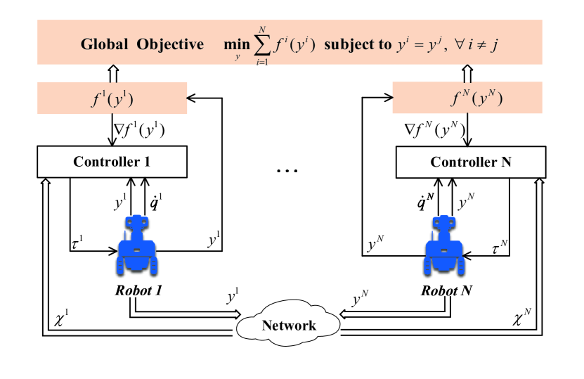
Figure 1: Schematic diagram of $N$ controlled EL systems, where $\chi^{i}=\textstyle{\sum}_{j\in\mathcal{N}_{i}}(y^{j}-y^{i})$ is the relative information received by $i$th agent from its neighbors. Only system output $y^{i}$ is available for neighboring agents via communication network.

To make the optimization problem solvable and stability analysis implementable, we have the following assumptions.

Assumption 2.1.

The undirected graph $\mathcal{G}$ is connected.  

Assumption 2.2.

The optimal value of problem (2), namely $f^{*}$, is finite and the optimal solution set

$$\mathcal{\textup{Y}}_{\mbox{\small{opt} }}=\left\{y=1_{N}\otimes z^{*}\mid\textstyle{\sum}_{i=1}^{N}f^{i}(z^{*})=f^{*}\right\}$$

is nonempty and compact  (Wang and Elia, , 2010).  

Assumption 2.3.

For $i\in\mathcal{V}$, the objective function $f^{i}$ is first-order differentiable, and $f^{i}$ as well as its measured gradient $\nabla f^{i}(y^{i})$ are only known to $i$th agent. Moreover, it is $\rho_{c}$-strongly convex and has $\varrho_{c}$-Lipschitz gradients, i.e., for $x_{1},x_{2}\in\mathbb{R}^{n}$,

$$(\nabla f^{i}(x_{1})-\nabla f^{i}(x_{2}))^{\scriptscriptstyle\top}(x_{1}-x_{2})\geq\rho_{c}\|x_{1}-x_{2}\|^{2},$$ (3)

$$\|\nabla f^{i}(x_{1})-\nabla f^{i}(x_{2})\|\leq\varrho_{c}\|x_{1}-x_{2}\|$$ (4)

where $\rho_{c}$ and $\varrho_{c}$ are some positive constants.  

Remark 2.1.

For $i\in\mathcal{V}$, if the local objective functions are defined as $f^{i}(y^{i})=(y^{i})^{\scriptscriptstyle\top}p^{i}y^{i}$ where $p^{i}$ is a positive definite matrix, then the gradient functions are given by $\nabla f^{i}(y^{i})=2p^{i}y^{i}$. In this paper, we assume that only output-dependent measured gradient values are available, specifically $2p^{i}y^{i}$. However, if each subsystem has a priori knowledge of the gradient function $\nabla f^{i}(\cdot)$, then $\nabla f^{i}(z^{i})=2p^{i}z^{i}$ can be computed for any $z^{i}\in\mathbb{R}^{n}$. With this information, we can design $z^{i}$-dynamics for each $i\in\mathcal{V}$ to cooperatively search for the optimal solution. Since the $z^{i}$-dynamics are independent of the subsystems, designing local tracking controllers becomes straightforward.  

Remark 2.2.

Compared to having a priori knowledge of the gradient function $\nabla f^{i}(\cdot)$, using output-dependent measured gradient values is more applicable in practical situations. For instance, in the source seeking problem  (Kim et al., , 2014), each robot cannot directly measure the distance to the source. Instead, they rely on radiation intensity sensors to estimate their proximity to the source. Similarly, in the problem of optimal formation control of multiple robots  (Wu et al., , 2022), robots measure their distances from one another in real-time to determine their next direction of movement, rather than generating an optimal trajectory beforehand and then tracking it.  

Remark 2.3.

Under Assumption 2.3, the strong convexity of local objective function $f^{i}(y^{i})$ implies its strict convexity. Therefore, the global objective function $\textstyle{\sum}_{i=1}^{N}f^{i}(y^{i})$ is strictly convex, since each $f^{i}(y^{i})$ is strictly convex for $i\in\mathcal{V}$. By Assumption 2.2, the optimal solution of optimization problem (2) is unique. In this paper, our proposed algorithm is also applicable when different local objective functions have distinct strongly convex constants $\rho_{c}^{i}$ and Lipschitz constants $\varrho_{c}^{i}$. In this scenario, inequalities (3) and (4) remain valid with $\rho_{c}=\min\{\rho_{c}^{1},\cdots,\rho_{c}^{N}\}$ and $\varrho_{c}=\max\{\varrho_{c}^{1},\cdots,\varrho_{c}^{N}\}$.  

The objective of the DPTCO is to design distributed controllers $u^{i},i\in\mathcal{V}$ using local output interactions $\chi^{i}=\textstyle{\sum}_{j\in\mathcal{N}_{i}}(y^{j}-y^{i})$ such that the outputs of all subsystems reach the optimal solution $y^{*}$ within a prescribed-time $T+t_{0}$ and remain at the optimal solution afterward, i.e.,

$$\lim_{t\to T+t_{0}}\|y(t)-y^{*}\|=0,$$ (5)

$$y(t)=y^{*},\quad t\geq T+t_{0}$$ (6)

where $y^{*}\in\textup{Y}_{\mbox{\small{opt} }}$. Furthermore, the position $y^{i}$, velocity $\dot{q}^{i}$ and control input $\tau^{i}$ must be uniformly bounded, i.e.,

$$\|\left[(y^{i}(t))^{\scriptscriptstyle\top},(\dot{q}^{i}(t))^{\scriptscriptstyle\top},(\tau^{i}(t))^{\scriptscriptstyle\top}\right]\|\in\mathcal{L}_{\infty}$$

holds for $i\in\mathcal{V}$ and $t\geq t_{0}$. The system structure for distributed feedback optimization is shown in Fig. 1.

2.3 Prescribed-time Analysis

We introduce the following time-varying functions which will be used to derive the prescribed-time convergence.

Definition 2.1.

Define $\mathbb{R}_{p}=[b,\infty)$ with $b\geq 0$. A continuous differentiable function $\mu(t):\mathcal{T}_{p}\mapsto\mathbb{R}_{p}$ is said to belong to class $\mathcal{K}_{T}$ if it is strictly increasing to infinity and

$$\frac{\mathrm{d}\mu(t)}{\mathrm{d}t}\Big{|}_{t=t_{0}}=b^{\prime},\quad\lim_{t\to T+t_{0}}\frac{\mathrm{d}\mu(t)}{\mathrm{d}t}=\infty,$$ (7)

$$\frac{\mathrm{d}\mu(t)}{\mathrm{d}t}\leq\tilde{b}(\mu(t))^{2},\quad\forall t\in\mathcal{T}_{p}$$ (8)

where $b^{\prime}$ and $\tilde{b}$ are some positive constant possibly related to $T$.  

Remark 2.4.

There are numerous functions $\mu(t)$ that belong to class $\mathcal{K}_{T}$. For instance, consider $\mu(t)=(T/(T+t_{0}-t))^{m}$ with $m\geq 1$. In this case, we have $b=1$, $b^{\prime}=m/T$ and $\tilde{b}=m/T$. Another example is $\mu(t)=\exp\left(1/(T+t_{0}-t)\right)$, where $b=\exp(1/T)$, $b^{\prime}=\exp\left(1/T\right)(1/T)^{2}$, and $\tilde{b}=4/\exp(2)$. It is also noteworthy that the asymptotic stability is recovered if $T$ is set to infinity.  

We simplify $\mu(t)$ and $\dot{\mu}(t)$ as $\mu$ and $\dot{\mu}$ throughout this paper if no confusion occurs and define

$$\kappa^{\iota}(\alpha(\mu))=\exp\left(\iota\textstyle{\int}_{t_{0}}^{t}\alpha(\mu(\tau))\mathrm{d}\tau\right),\;t\geq t_{0},$$ (9)

$$\kappa^{\iota}(\alpha(\mu(\tau)))=\exp\left(\iota\textstyle{\int}_{t_{0}}^{\tau}\alpha(\mu(s))\mathrm{d}s\right),\;\tau\geq t_{0}$$ (10)

where $\iota$ is constant and $\alpha\in\mathcal{K}_{\infty}$. We note $\kappa^{\iota}(\alpha(\mu))$ converges to zero as $t\to T+t_{0}$ for any $\iota<0$ and $\alpha\in\mathcal{K}_{\infty}$.

Definition 2.2.

A function $\alpha:[0,\infty)\mapsto[b,\infty)$ is said to belong to class $\mathcal{K}_{\infty}^{e}$, if it is strictly increasing and $\alpha(0)=b>0$.  

Definition 2.3.

A continuous function $\beta:[0,\infty)\times[0,\infty)\mapsto[0,\infty)$ is said to belong class $\mathcal{KL}_{T}$ if, for each fixed $s$, the mapping $\beta(r,s)$ belongs to class $\mathcal{K}_{\infty}$ with respect to $r$ and, for each fixed $r$, there exists a constant $T$ such that, for $s\in[0,T)$, the mapping $\beta(r,s)$ is decreasing with respect to $s$ and satisfies $\beta(r,s)\to 0$ as $s\to T$, $\beta(r,s)=0$ for $s\in[T,\infty)$. In addition, the function $\beta$ is said to belong class $\mathcal{KL}_{T}^{e}$ if, for each fixed $s$, the mapping $\beta(r,s)$ belongs to class $\mathcal{K}_{\infty}^{e}$ with respect to $r$.  

Definition 2.4.

Consider the system

$$\dot{\chi}=g(t,\chi,d(t)),\quad\chi(t_{0})=\chi_{0}$$ (11)

where $\chi\in\mathbb{R}^{n}$ is the state, $d(t):[t_{0},\infty)\mapsto\mathbb{R}^{n_{d}}$ is the external input, and $\chi_{0}$ is the initial state at initial time $t_{0}$. For any given $T>0$, the $\chi$-dynamics is said to be prescribed-time stable if there exits $\beta\in\mathcal{KL}_{T}^{e}$ such that, for any $\chi_{0}\in\mathbb{R}^{n}$, $d\in\mathbb{R}^{n_{d}}$,

$$\|\chi(t)\|\leq\beta(\|\chi_{0}\|,t-t_{0})$$

holds for $t_{0}\leq t<\infty$.  

Definition 2.5.

The continuously differentiable function $V(\chi):\mathbb{R}^{n}\mapsto\mathbb{R}_{+}$ is called the prescribed-time input-to-state stable (ISS) Lyapunov function for system in (11) with $d$ being the input, if $V(\chi)$ and its derivative along the trajectory of the system satisfy, for all $\chi\in\mathbb{R}^{n}$ and $t\in\mathcal{T}_{p}$,

$$\begin{gathered}\underline{\alpha}(\|\chi\|)\leq V(\chi)\leq\overline{\alpha}(\|\chi\|),\\ \dot{V}\leq-\alpha(\mu)V+\tilde{\epsilon}(\mu)\epsilon(\|d\|)\end{gathered}$$ (12)

where $\underline{\alpha}$, $\overline{\alpha}$, $\alpha$, $\tilde{\epsilon}$, $\epsilon\in\mathcal{K}_{\infty}$. $\alpha(\mu)$, $\tilde{\epsilon}(\mu)$ and $\epsilon(\|d\|)$ are called prescribed-time convergent gain, prescribed-time ISS gain and (normal) ISS gain, respectively. The inequalities in (12) are simplified as $V(\chi)\sim\{\underline{\alpha},\overline{\alpha},\alpha,[\epsilon(\|d\|),\tilde{\epsilon}]\mid\dot{\chi}=g(t,\chi,d)\}$. When system (11) has multiple inputs, i.e., $\dot{\chi}=g(t,\chi,d_{1}(t),\cdots,d_{n}(t))$ where $d_{i}\in\mathbb{R}^{n_{di}}$, the second inequality of (12) becomes $\dot{V}\leq-\alpha(\mu)V+\textstyle{\sum}\tilde{\epsilon}_{i}(\mu)\epsilon_{i}(\|d_{i}\|),$ and the inequalities are simplified as $V(\chi)\sim\{\underline{\alpha},\overline{\alpha},\alpha,[\epsilon_{1}(\|d_{1}\|),\tilde{\epsilon}_{1}],\cdots,[\epsilon_{n}(\|d_{n}\|),\tilde{\epsilon}_{n}]\mid\dot{\chi}=g(t,\chi,d_{1},\cdots,d_{n})\}$.  

Definition 2.6.

A time-varying mapping nonlinear mapping $h(\chi,\mu):\mathbb{R}^{n}\times\mathbb{R}_{p}\mapsto\mathbb{R}^{m}$ is said to be a prescribed-time mapping if the partial derivatives $\frac{\partial h(\chi,\mu)}{\partial\chi}$ and $\frac{\partial h(\chi,\mu)}{\partial\mu}$ exist. Additionally, if $h(\chi,\mu)$ is uniformly bounded for $t\in\mathcal{T}_{p}$, this uniform boundedness guarantees the prescribed-time convergence of $\chi$.  

Remark 2.5.

The prescribed-time mapping is a very useful tool in deriving prescribed-time stabilization of a dynamic system. For example, consider a disturbed system $\dot{\chi}=-k\mu\chi+d(t)$, where $\chi\in\mathbb{R}^{n}$, $k>0$, $\mu\in\mathcal{K}_{T}$, and $d(t)\in\mathbb{R}^{n}$ satisfying $\sup_{t\geq t_{0}}\|d(t)\|\leq\bar{d}$ . Define the Lyapunov function candidate for $\chi$-dynamics as $V(\chi)=\frac{1}{2}\chi^{\scriptscriptstyle\top}\chi$, then its time derivative satisfies $\dot{V}(\chi)=-k\mu\|\chi\|^{2}+\chi^{\scriptscriptstyle\top}d(t)\leq(-2k\mu+1)V(\chi)+\bar{d}^{2}/2$. Invoking comparison lemma yields

$$V(\chi(t)) \leq\kappa^{-2k}(\mu)\exp\left(t-t_{0}\right)V(\chi(t_{0}))$$

$$\quad+\frac{\bar{d}^{2}}{2}\kappa^{-2k}(\mu)\textstyle{\int}_{t_{0}}^{t}\kappa^{2k}(\mu(\tau))\exp(t-\tau)\mathrm{d}\tau$$

where $\kappa(\mu)$ and $\kappa(\mu(\tau))$ are defined in (9) and (10). Observing the upper bound of $V(\chi)$, it is both tedious and complicated to analyze the prescribed-time convergence of $V(\chi)$ as well as $\chi$. By applying the prescribed-time mapping, we define $\tilde{\chi}=h(\chi,\mu)=\mu\chi$. The $\tilde{\chi}$-dynamics is given by $\dot{\tilde{\chi}}=(-k\mu+\dot{\mu}/\mu)\tilde{\chi}+\mu d(t)$. We define the Lyapunov function candidate for $\tilde{\chi}$-dynamics as $\tilde{V}(\tilde{\chi})=\frac{1}{2}\tilde{\chi}^{\scriptscriptstyle\top}\tilde{\chi}$ and assume $k\geq\frac{k^{*}}{2}+\tilde{b}+\frac{1}{2}$, where $\tilde{b}$ is denoted in (8). Upon using Young’s inequality, the time derivative satisfies $\dot{\tilde{V}}(\tilde{\chi})\leq-k^{*}\mu\tilde{V}(\tilde{\chi})+\frac{1}{2}\mu\bar{d}^{2}$. Invoking comparison lemma yields $\tilde{V}(\tilde{\chi}(t))\leq\kappa^{-k^{*}}(\mu)\left(\tilde{V}(\tilde{\chi}(t_{0}))-\frac{\bar{d}^{2}}{2k^{*}}\right)+\frac{\bar{d}^{2}}{2k^{*}}\leq\tilde{V}(\tilde{\chi}(t_{0}))+\frac{\bar{d}^{2}}{2k^{*}}$, which further implies the prescribed-time convergence of the original state $\chi$, i.e., $\|\chi(t)\|\leq\left(\mu(t_{0})^{2}\|\chi(t_{0})\|^{2}+\bar{d}^{2}/k^{*}\right)^{\frac{1}{2}}\mu^{-1}(t)$.  

3 DPTCO Algorithm Design and Coordinate Transformations

Given that the relative degree of each subsystem in (1) is greater than one, directly proving whether the output of the closed-loop system can converge to the optimal solution is a very complicated problem. Instead, we construct auxiliary systems to seek the optimal solution, with these seeking trajectories considered as reference trajectories for local subsystems. The DPTCO problem is then divided into two parts: distributed optimal solution seeking and local reference trajectory tracking.

For $i\in\mathcal{V}$ and , the auxiliary systems are designed as follows:

$$\dot{\varpi}^{i}(t) =-c\mu\left(\nabla f^{i}(y^{i})+\chi_{y}^{i}+v^{i}\right),$$ (13)

$$\dot{v}^{i}(t) =c\mu\chi_{y}^{i},\quad t\in\mathcal{T}_{p}$$ (14)

where $c>0$ is a design parameter, $\mu\in\mathcal{K}_{T}$ is denoted in Definition 2.1, and $\chi_{y}^{i}=\textstyle{\sum}_{j\in\mathcal{N}_{i}}a_{ij}(y^{i}-y^{i})$ represents the relative information received by $i$th subsystem. Additionally,

$$\dot{\varpi}^{i}(t)=0,\quad\dot{v}^{i}(t)=0,\quad t\in\tilde{\mathcal{T}}_{p}.$$ (15)

$\varpi^{i}\in\mathbb{R}^{n}$ aims to converge to $z^{*}$ within $T+t_{0}$ and remain as $z^{*}$ afterward, $v^{i}\in\mathbb{R}^{n}$ is designed to adaptively find the value $\nabla f^{i}(z^{*})$.

Based on auxiliary systems (13)-(15), for $i\in\mathcal{V}$, the local prescribed-time tracking controller is designed as

$$\tau^{i}(t)=\begin{cases}\pi^{i}(q^{i},\dot{q}^{i},\varpi^{i},\hat{\theta}^{i},\mu),&\mbox{for}\;t\in\mathcal{T}_{p}\\ 0,&\mbox{for}\;t\in\tilde{\mathcal{T}_{p}}\end{cases}$$ (16)

where

$$\pi^{i}(q^{i},\dot{q}^{i},\varpi^{i},\hat{\theta}^{i},\mu)$$

$$=-k_{2}^{i}\mu(\dot{q}^{i}+k_{1}^{i}\mu(y^{i}-\varpi^{i}))-\Omega^{i}(q^{i},\dot{q}^{i},z_{1}^{i},z_{2}^{i})\hat{\theta}^{i}$$ (17)

and $k_{1}^{i}$, $k_{2}^{i}$ are design parameters. The matrix function $\Omega^{i}(q^{i},\dot{q}^{i},z_{1}^{i},z_{2}^{i})$ can be calculated according to Property 2.2, with $z_{1}^{i}$, $z_{2}^{i}$ being intermediate variables denoted as

$$z_{1}^{i} =\left((\iota-1)\tilde{\mu}+k_{1}^{i}\mu\right)\dot{q}^{i}+\iota k_{1}^{i}\mu\tilde{\mu}(y^{i}-\varpi^{i}),$$ (18)

$$z_{2}^{i} =k_{1}^{i}\mu(y^{i}-\varpi^{i})$$ (19)

where $\iota>0$ is a design parameter and $\tilde{\mu}=\dot{\mu}/\mu$. In (16), $\hat{\theta}^{i}\in\mathbb{R}^{p}$ denotes the estimate of unknown parameter $\theta^{i}$ whose dynamics is designed as

$$\dot{\hat{\theta}}^{i}=\varsigma^{i}(q^{i},\dot{q}^{i},\varpi^{i},\mu)-\sigma^{i}\mu\hat{\theta}^{i}$$ (20)

for $i\in\mathcal{V}$ and $t\in\mathcal{T}_{p}$, where $\sigma^{i}\geq\tilde{b}$ is a design parameter and

$$\varsigma^{i}(q^{i},\dot{q}^{i},\varpi^{i},\mu)$$

$$=2\mu^{2\iota-2}\left(\Omega^{i}(q^{i},\dot{q}^{i},z_{1}^{i},z_{2}^{i})\right)^{\scriptscriptstyle\top}(\dot{q}^{i}+k_{1}^{i}\mu(y^{i}-\varpi^{i})).$$ (21)

We note that $\hat{\theta}^{i}(t)$ only exists for $t\in\mathcal{T}_{p}$. Define

$$\tilde{\theta}^{i}=\theta^{i}-\hat{\theta}^{i}$$

as the estimate error for $i\in\mathcal{V}$.

Let $y^{i}=\varpi^{i}$, $\dot{q}^{i}=0$, one has $z_{1}^{i}=0$ and $z_{2}^{i}=0$, then by Property 2.2, $\pi^{i}(q^{i},\dot{q}^{i},\varpi^{i},\hat{\theta}^{i},\mu)$ satisfies $\pi^{i}(\varpi^{i},0,\varpi^{i},\hat{\theta}^{i},\mu)=0$ for any $\hat{\theta}^{i}\in\mathbb{R}^{p}$ and $\mu\in\mathbb{R}_{p}$.

Define the lumped vectors $\varpi=[(\varpi^{1})^{\scriptscriptstyle\top},\cdots,(\varpi^{N})^{\scriptscriptstyle\top}]^{\scriptscriptstyle\top}$, $v=[(v^{1})^{\scriptscriptstyle\top},\cdots,(v^{N})^{\scriptscriptstyle\top}]^{\scriptscriptstyle\top}$, $\dot{q}=[(\dot{q}^{1})^{\scriptscriptstyle\top},\cdots,(\dot{q}^{N})^{\scriptscriptstyle\top}]^{\scriptscriptstyle\top}$, $\hat{\theta}=[(\hat{\theta}^{1})^{\scriptscriptstyle\top},\cdots,(\hat{\theta}^{N})^{\scriptscriptstyle\top}]^{\scriptscriptstyle\top}$ and $\dot{\hat{\theta}}=[(\dot{\hat{\theta}}^{1})^{\scriptscriptstyle\top},\cdots,(\dot{\hat{\theta}}^{N})^{\scriptscriptstyle\top}]^{\scriptscriptstyle\top}$, then according to (1), (13), (14) and (17), for $t\in\mathcal{T}_{p}$, the closed-loop NELSs can be written in a compact form as

$$\dot{\varpi}(t) =-c\mu\nabla F(y)-c\mu\bar{\mathcal{L}}y-c\mu v,$$ (22)

$$\dot{v}(t) =c\mu\bar{\mathcal{L}}y,$$ (23)

$$\dot{y}(t) =\dot{q},$$ (24)

$$\ddot{q}(t) =M^{-1}(q)(\pi(q,\dot{q},\varpi,\hat{\theta},\mu)-C(q,\dot{q})\dot{q}),$$ (25)

$$\dot{\hat{\theta}}(t) =\varsigma(q,\dot{q},\varpi,\mu)-\bar{\sigma}\mu\hat{\theta}$$ (26)

where $\bar{\mathcal{L}}=\mathcal{L}\otimes I_{n}$, $M=\mbox{diag}\{M^{1},\cdots,M^{N}\}$, $\pi=[(\pi^{1})^{\scriptscriptstyle\top},\cdots,(\pi^{N})]^{\scriptscriptstyle\top}$ with $\pi^{i}$ denoted in (16), $C=\mbox{diag}\{C^{1},\cdots,C^{N}\}$, $\nabla F(y)=[(\nabla f^{1}(y^{1}))^{\scriptscriptstyle\top},\cdots,(\nabla f^{N}(y^{N}))^{\scriptscriptstyle\top}]^{\scriptscriptstyle\top}$, $\varsigma=[(\varsigma^{1})^{\scriptscriptstyle\top},\cdots,(\varsigma^{N})^{\scriptscriptstyle\top}]^{\scriptscriptstyle\top}$ and $\bar{\sigma}=\mbox{diag}\{\sigma^{1},\cdots,\sigma^{N}\}\otimes I_{p}$. Define

$$\eta=\left[c,\iota,k_{1}^{\scriptscriptstyle\top},k_{2}^{\scriptscriptstyle\top},\sigma^{\scriptscriptstyle\top}\right]^{\scriptscriptstyle\top}\in\mathbb{R}^{3N+2}$$ (27)

as the vector contains all design parameters of the whole controlled system, where $k_{1}=[k_{1}^{1},\cdots,k_{1}^{N}]^{\scriptscriptstyle\top}$, $k_{2}=[k_{2}^{1},\cdots k_{2}^{N}]^{\scriptscriptstyle\top}$ and $\sigma=[\sigma^{1},\cdots,\sigma^{N}]^{\scriptscriptstyle\top}$.

Proposition 3.1.

Let the optimal solution of optimization problem (2) is $y^{*}=1_{N}\otimes z^{*}$ for some $z^{*}\in\mathbb{R}^{n}$. Suppose Assumption 2.1, 2.2 hold and the initial value of $v^{i}$ satisfies $\textstyle{\sum}_{i=1}^{N}v^{i}(t_{0})=0$, then the equilibrium points of system (22)-(25) are

$$\varpi^{*}=1_{N}\otimes z^{*},\quad v^{*}=-\nabla F(1_{N}\otimes z^{*}),$$ (28)

$$y^{*}=1_{N}\otimes z^{*},\quad\dot{q}^{*}=0$$ (29)

where $\nabla F(1_{N}\otimes z^{*})=\left[(\nabla f^{1}(z^{*}))^{\scriptscriptstyle\top},\cdots,(\nabla f^{N}(z^{*}))^{\scriptscriptstyle\top}\right]^{\scriptscriptstyle\top}$.  

Proof: Consider the solution of

$$\begin{cases}0=-c\mu\nabla F(y)-c\mu\bar{\mathcal{L}}y-c\mu v\\ 0=c\mu\bar{\mathcal{L}}y\\ 0=\dot{q}\\ 0=M^{-1}(q)(\pi(q,\dot{q},\varpi,\hat{\theta},\mu)-C(q,\dot{q})\dot{q})\end{cases}$$ (30)

where we omit (26) since the value of $\hat{\theta}$ at the equilibrium point does not impact the equilibrium points of other variables. By the second and third equations of (30), one has $\dot{q}^{*}=0$ and $y^{*}=1_{N}\otimes\zeta$ for some $\zeta\in\mathbb{R}^{n}$. Since $\mathcal{G}$ is undirected and connected, the Laplacian matrix $\mathcal{L}$ is symmetric and its null space is spanned by $1_{N}$, then $1_{N}^{\scriptscriptstyle\top}\mathcal{L}=0$. By $\textstyle{\sum}_{i=1}^{N}v^{i}(t_{0})=0$, for $t\in\mathcal{T}_{p}$,

$$(1_{N}^{\scriptscriptstyle\top}\otimes I_{n})v(t)$$

$$=(1_{N}^{\scriptscriptstyle\top}\otimes I_{n})v(t_{0})+\textstyle{\int}_{t_{0}}^{t}(1_{N}^{\scriptscriptstyle\top}\otimes I_{n})\dot{v}(\tau)\mathrm{d}\tau$$

$$=\textstyle{\sum}_{i=1}^{N}v^{i}(t_{0})+\textstyle{\int}_{t_{0}}^{t}(1_{N}^{\scriptscriptstyle\top}\mathcal{L}\otimes I_{n})c\mu(\tau)y(\tau)\mathrm{d}\tau$$

$$=0.$$

Left multiplying the first inequality in (30) by $1_{N}^{\scriptscriptstyle\top}\otimes I_{n}$ yields $\textstyle{\sum}_{i=1}^{N}\nabla f^{i}(\zeta)=0$. For the optimization problem (2), the necessary and sufficient condition for a point $1_{N}\otimes z^{*}$ to be the optimal solution is $\textstyle{\sum}_{i=1}^{N}\nabla f^{i}(z^{*})=0$  (Kia et al., , 2015). Thus we have $\zeta=z^{*}$ and $v^{*}=-\nabla F(1_{N}\otimes z^{*})$. Note that $\pi(\varpi,0,\varpi,\hat{\theta},\mu)=0$ and $q=y$, then the forth equality in (30) leads to $\varpi^{*}=1_{N}\otimes z^{*}$.  

Define error variables as

$$e_{\varpi} =\varpi-1_{N}\otimes z^{*},$$ (31)

$$e_{v} =v+\nabla F(1_{N}\otimes z^{*}),$$ (32)

$$e_{y} =y-\varpi$$ (33)

and

$$e_{r}=\left[e_{\varpi}^{\scriptscriptstyle\top},e_{v}^{\scriptscriptstyle\top}\right]^{\scriptscriptstyle\top},\quad e_{s}=\left[e_{y}^{\scriptscriptstyle\top},\dot{q}^{\scriptscriptstyle\top}\right]^{\scriptscriptstyle\top}.$$ (34)

Based on Proposition 3.1, the DPTCO problem is converted into the prescribed-time stabilization problem of $e_{r}$ and $e_{s}$.

Remark 3.1.

The proof of Proposition 3.1 implies that the implementation of the DPTCO with a feedback approach requires a precondition: the controlled NELSs in (1) must have an equilibrium point at $[(q^{i,})^{\scriptscriptstyle\top},(\dot{q}^{i,})^{\scriptscriptstyle\top}]^{\scriptscriptstyle\top}=[(\zeta^{i,})^{\scriptscriptstyle\top},0_{n}^{\scriptscriptstyle\top}]^{\scriptscriptstyle\top}$ for any $\zeta^{i,}\in\mathbb{R}^{n}$ and $i\in\mathcal{V}$. This necessitates that the equilibrium point for each robot be position-independent. Consequently, system (1) assumes that each robot is moving in the horizontal direction or that the gravitational torque has already been compensated for through feedforward control. Furthermore, the adaptive estimation $\hat{\theta}^{i}$ in (17) is introduced to ensure that $\pi^{i}(\varpi^{i},0,\varpi^{i},\hat{\theta}^{i},\mu)=0$ for any $\hat{\theta}^{i}\in\mathbb{R}^{p}$ and $\mu\in\mathbb{R}_{p}$. This condition is crucial to extend the prescribed-time control indefinitely and ensure the continuity of the control inputs over the global time interval.  

4 Interconnected Error System and Prescribed-Time Small-Gain criterion

In this section, we show that the feedback approach based DPTCO problem, along with the boundedness issue of internals signals in the closed-loop systems, can be converted into the practical stability problem of an interconnected system. Subsequently, we propose a prescribed-time small-gain criterion to delineate the conditions necessary for ensuring practical stability.

4.1 Interconnected Error System and Prescribed-Time Mapping

To make controllers in (16) implementable, the adaptive estimate $\hat{\theta}^{i}(t)$ must be bounded for $t\in\mathcal{T}_{p}$ and $i\in\mathcal{V}$. It is equivalent to proving the uniform boundedness of the estimation error $\tilde{\theta}^{i}$ since $\theta^{i}$ is a finite constant vector. Furthermore, since $\mu(t)$ increases to infinity as $t\to T+t_{0}$, the proposed design must guarantee uniform boundedness of the $\mu(t)$-dependent terms in (13), (14), (16) and (20). This issue can be addressed by further exploiting the prescribed-time convergence rate of $e_{r}$ and $e_{s}$. For example, from (22), (23), and (31)-(34), one has

$$\|\dot{e}_{r}\|\leq c(2\lambda_{N}+\varrho_{c}+1)\mu(\|e_{r}\|+\|e_{y}\|)$$ (35)

which implies that to guarantee the uniform boundedness of $\dot{\varpi}^{i}$ and $\dot{v}^{i}$ for $i\in\mathcal{V}$ and $t\in\mathcal{T}_{p}$, $e_{r}$ and $e_{s}$ must achieve prescribed-time convergence rate no less than $\mu^{-1}(t)$. As explained in Remark 2.5, it is impractical to directly analyze the prescribed-time convergence as well as prescribed-time convergence rate of $e_{r}$ and $e_{s}$ through their dynamics. Therefore, we introduce the following time-varying state transformations, for $t\in\mathcal{T}_{p}$,

$$\tilde{e}_{r}=\mu^{\iota}e_{r},\quad\tilde{e}_{s}=\Lambda_{1}(\mu)e_{s}$$ (36)

where $\iota$ is introduced in (18) and

$$\Lambda_{1}(\mu)=\left[\begin{array}[]{cc}\mu^{\iota}I_{nN}&0_{nN\times nN}\\ \mu^{\iota}\bar{K}_{1}&\mu^{\iota-1}I_{nN}\end{array}\right]$$

where $\bar{K}_{1}=K_{1}\otimes I_{n}\in\mathbb{R}^{nN\times nN}$ with $K_{1}=\mbox{diag}\{k_{1}^{1},\cdots,k_{1}^{N}\}$. According to (1), (20), (22) and (23), for $t\in\mathcal{T}_{p}$, the dynamics of $\tilde{e}_{r}$, $\tilde{e}_{s}$ and $\tilde{\theta}$ can be expressed as

$$\dot{\tilde{e}}_{r}=\zeta_{r}(\tilde{e}_{r},\tilde{e}_{s},\mu),$$ (37)

$$\dot{\tilde{e}}_{s}=\zeta_{s}(\tilde{e}_{r},\tilde{e}_{s},\tilde{\theta},\mu),$$ (38)

$$\dot{\tilde{\theta}}=\zeta_{\theta}(\tilde{e}_{s},\tilde{\theta},\mu)$$ (39)

where

$$\zeta_{r}(\tilde{e}_{r},\tilde{e}_{s},\mu)=\iota\tilde{\mu}\tilde{e}_{r}+c\mu^{\iota+1}$$

$$\times\left[\begin{gathered}-\bar{\mathcal{L}}(e_{\varpi}+e_{y})-e_{v}-\nabla\tilde{F}(y,\varpi)-\nabla\tilde{F}(\varpi,\varpi^{*})\\ \bar{\mathcal{L}}e_{y}+\bar{\mathcal{L}}e_{\varpi}\end{gathered}\right],$$

$$\zeta_{s}(\tilde{e}_{r},\tilde{e}_{s},\mu)=\tilde{\mu}\left[\begin{array}[]{cc}\iota I_{nN}&0_{nN\times nN}\\ \bar{K}_{1}&(\iota-1)I_{nN}\end{array}\right]\tilde{e}_{s}$$

$$+\Lambda_{1}(\mu)\left[\begin{array}[]{c}\dot{q}-\dot{\varpi}\\ M^{-1}(q)(\pi(q,\dot{q},\varpi,\hat{\theta},\mu)-C(q,\dot{q})\dot{q})\end{array}\right],$$

$$\begin{aligned} \zeta_{\theta}(\tilde{e}_{s},\tilde{\theta},\mu)&=\bar{\sigma}\mu(\theta-\tilde{\theta})\\ &\quad-2\mu^{\iota-1}\left(\Omega(q,\dot{q},z_{1},z_{2})\right)^{\scriptscriptstyle\top}\left[0,I_{nN}\right]\tilde{e}_{s}\end{aligned}$$

where $\Omega=\mbox{diag}\left\{\Omega^{1},\cdots,\Omega^{N}\right\}$ and we used the facts $\bar{\mathcal{L}}(1_{N}\otimes z^{*})=0$ and

$$\dot{e}_{\varpi} =-c\mu\nabla F(y)-c\alpha(\mu)\bar{\mathcal{L}}y-c\alpha(\mu)v$$

$$=-c\mu\big{(}\bar{\mathcal{L}}e_{\varpi}+\bar{\mathcal{L}}e_{y}+e_{v}+\nabla\tilde{F}(y,\varpi)$$

$$\quad+\nabla\tilde{F}(\varpi,\varpi^{*})\big{)}$$ (40)

where $\nabla\tilde{F}(y,\varpi)$ and $\nabla\tilde{F}(\varpi,\varpi^{*})$ are denoted by

$$\nabla\tilde{F}(y,\varpi)= \left[(\nabla f^{1}(y^{1})-\nabla f^{1}(\varpi^{1}))^{\scriptscriptstyle\top},\right.$$

$$\left.\cdots,(\nabla f^{N}(y^{N})-\nabla f^{N}(\varpi^{N}))^{\scriptscriptstyle\top}\right]^{\scriptscriptstyle\top},$$

$$\nabla\tilde{F}(\varpi,\varpi^{*})= \left[(\nabla f^{1}(\varpi^{1})-\nabla f^{1}(z^{*}))^{\scriptscriptstyle\top},\right.$$

$$\left.\cdots,(\nabla f^{N}(\varpi^{N})-\nabla f^{N}(z^{*}))^{\scriptscriptstyle\top}\right]^{\scriptscriptstyle\top}.$$

By examining (37)-(39), we observe that the dynamics of $\tilde{e}_{r}$, $\tilde{e}_{s}$ and $\tilde{\theta}$ are in an interconnected form.

We have the following lemma, whose proof is given in appendix.

Lemma 4.1.

The time-varying state transformation (36) serves as a prescribed-time mapping from $e_{r}$, $e_{s}$ to $\tilde{e}_{r}$, $\tilde{e}_{s}$ if $\iota>2$. For $t\in\mathcal{T}_{p}$, the uniform boundedness of $\tilde{e}_{r}$ and $\tilde{e}_{s}$ imply the prescribed-time convergence of $e_{r}$ and $e_{s}$ with the upper bounds

$$\|e_{r}\|\leq\mu^{-\iota}\gamma_{r}(\|\tilde{e}_{r}\|_{\mathcal{T}}),\quad\|e_{s}\|\leq\mu^{-\iota+1}\gamma_{s}(\|\tilde{e}_{s}\|_{\mathcal{T}})$$ (41)

where $\|\tilde{e}_{r}\|_{\mathcal{T}}=\sup_{t\in\mathcal{T}_{p}}\|\tilde{e}_{r}\|$, $\|\tilde{e}_{s}\|_{\mathcal{T}}=\sup_{t\in\mathcal{T}_{p}}\|\tilde{e}_{s}\|$ and $\gamma_{r},\gamma_{s}\in\mathcal{K}_{\infty}$. Furthermore, if $\tilde{e}_{r}$ and $\tilde{e}_{s}$ are uniformly bounded, then $\dot{\varpi}^{i}$, $\dot{v}^{i}$ in (22) and (23), controller $\tau^{i}$ in (16), and adaptive estimate $\hat{\theta}^{i}$ as well as its dynamics $\dot{\hat{\theta}}^{i}$ in (20) are uniformly bounded for $t\in\mathcal{T}_{p}$ and $i\in\mathcal{V}$.  

4.2 Prescribed-time small-gain criterion

Based on Lemma 4.1, the DPTCO problem is now converted into the uniform boundedness problem of $\tilde{e}_{r}$ and $\tilde{e}_{s}$. To facilitate the prescribed-time stability analysis and provide an analytical method for selecting control parameters, we introduce the following prescribed-time small-gain criterion, whose proof is given in appendix.

Theorem 4.1.

Consider the system

$$\begin{gathered}\dot{\chi}_{1}=h_{1}(t,\chi_{1},\chi_{2},d_{1}(t)),\\ \dot{\chi}_{2}=h_{2}(t,\chi_{1},\chi_{2},d_{2}(t))\end{gathered}$$ (42)

where $\chi=[\chi_{1}^{\scriptscriptstyle\top},\chi_{2}^{\scriptscriptstyle\top}]^{\scriptscriptstyle\top}\in\mathbb{R}^{n_{1}}\times\mathbb{R}^{n_{2}}$ is the state with $\chi_{0}=[\chi_{1}^{\scriptscriptstyle\top}(t_{0}),\chi_{2}^{\scriptscriptstyle\top}(t_{0})]^{\scriptscriptstyle\top}$ as the initial value, and $d_{i}(t):[t_{0},\infty)\mapsto\mathbb{D}_{i}$ is the external disturbance for $i=1,2$, where $\mathbb{D}_{i}$ is a compact set belonging to $\mathbb{R}^{l_{i}}$. Each $\chi_{i}$-subsystem admits a prescribed-time ISS Lyapunov function $V_{i}(\chi_{i})$ in the form of Definition 2.5 with $d_{i}$ and $\chi_{3-i}$ as the inputs, i.e.,

$$V_{1}(\chi_{1})\sim\left\{\underline{\alpha}_{1},\overline{\alpha}_{1},\alpha_{1},[V_{2}(\chi_{2}),l_{1}\alpha_{2}],[\epsilon_{1}(\|d_{1}\|),\gamma_{1}]\right\}$$ (43)

$$V_{2}(\chi_{2})\sim\left\{\underline{\alpha}_{2},\overline{\alpha}_{2},\alpha_{2},[V_{1}(\chi_{1}),l_{2}\alpha_{1}],[\epsilon_{2}(\|d_{2}\|),\gamma_{2}]\right\}$$ (44)

where $\underline{\alpha}_{i}$, $\overline{\alpha}_{i}$, $\alpha_{i}$, $\gamma_{i}$, $\epsilon_{i}\in\mathcal{K}_{\infty}$, and $l_{i}$ is positive a finite constant for $i=1,2$. If

$$l_{1}l_{2}<1,$$ (45)

$$\min\{\alpha_{1}(s),\alpha_{2}(s)\}=\mathcal{O}\left[\gamma_{1}(s)+\gamma_{2}(s)\right]$$ (46)

hold for $s\in\mathbb{R}_{+}$, then $\chi$ is uniformly bounded for $t\in\mathcal{T}_{p}$ with upper bound

$$\|\chi\|\leq\tilde{\alpha}(\|\chi_{0}\|)$$ (47)

where $\tilde{\alpha}$ is some $\mathcal{K}_{\infty}^{e}$ function.  

Remark 4.1.

In contrast to asymptotic stabilization  (Jiang and Liu, , 2018) and finite-time stabilization  (Pavlichkov, , 2018; Li et al., , 2024), the prescribed-time stabilization of an interconnected system requires not only that the coupling parts of prescribed-time ISS Lyapunov functions meet the small-gain condition (45), but also specific condition on the relationship between prescribed-time convergent gain and prescribed-time ISS gain with respect to external disturbance, see (46) for details.  

Remark 4.2.

For Theorem 4.1, if (45) holds and (46) is modified to $\min\{\alpha_{1}(s),\alpha_{2}(s)\}=\mathcal{O}\left[\tilde{\gamma}(s)(\gamma_{1}(s)+\gamma_{2}(s))\right]$ for some $\tilde{\gamma}\in\mathcal{K}_{\infty}$, then all results in Theorem 4.1 still hold. Additionally, $\chi$ satisfies $\|\chi(t)\|\leq(\tilde{\gamma}^{\prime}\circ\tilde{\gamma}(\mu))^{-1}\tilde{\alpha}^{\prime}(\|\chi(t_{0}))\|$ for some $\tilde{\gamma}^{\prime}\in\mathcal{K}_{\infty}$ and $\tilde{\alpha}^{\prime}\in\mathcal{K}_{\infty}^{e}$, which implies that $\chi$ achieves prescribed-time convergence towards zero in the presence of any bounded external disturbances. This highlights the robustness advantage of prescribed-time control over asymptotic and finite-time control.  

5 DPTCO Implementation

Through the application of time-varying state transformation (36) and Lemma 4.1, the implementation of the DPTCO, as well as the uniform boundedness of all internal signals, now hinges on the boundedness of $\tilde{e}_{r}$ and $\tilde{e}_{s}$. In this section, we elaborate on the parameter design and provide a detailed stability analysis of the dynamics of $\tilde{e}_{r}$ and $\tilde{e}_{s}$.

5.1 The Prescribed-Time ISS Lyapunov Functions

Due to the introduction of adaptive estimation $\hat{\theta}$, it is essential to incorporate a positive definite, differentiable term with respect to estimation error $\tilde{\theta}$ in the corresponding Lyapunov function. Therefore, we define

$$\tilde{e}_{s}^{\prime}=[\tilde{e}_{s}^{\scriptscriptstyle\top},\tilde{\theta}^{\scriptscriptstyle\top}]^{\scriptscriptstyle\top}.$$ (48)

Then according to Lemma 4.1 and Theorem 4.1, for $t\in\mathcal{T}_{p}$, the DPTCO is achieved if the dynamics of $\tilde{e}_{r}$- and $\tilde{e}_{s}^{\prime}$ admit prescribed-time ISS Lyapunov functions as described in (43) and (44). Additionally, the design parameter $\eta$ in (27) must ensure that conditions (45) and (46) are satisfied. For simplicity, define $\bar{k}_{\overline{m}}=\max\{k_{\overline{m}}^{1},\cdots,k_{\overline{m}}^{N}\}$, $\underline{k}_{\underline{m}}=\min\{k_{\underline{m}}^{1},\cdots,k_{\underline{m}}^{N}\}$ and

$$\begin{gathered}\delta=\max\{4/\lambda_{2},(4\varrho_{c}^{2}+1)/\rho_{c}\},\\ \bar{\varepsilon}=\max\left\{1,\bar{k}_{\overline{m}}\right\},\quad\underline{\varepsilon}=\min\left\{1,\underline{k}_{\underline{m}}\right\},\\ \bar{\delta}=\delta\max\{1,\lambda_{2}^{-1}\}/2+1/2,\quad\underline{\delta}=\delta\min\{1,\lambda_{N}^{-1}\}/2.\end{gathered}$$ (52)

Then we proposed the following design criteria for parameter $\eta$ in (27).

$\textbf{DC}_{\textbf{1}}$: $\iota$ in (18) is any any constant satisfying $\iota>2$;

$\textbf{DC}_{\textbf{2}}$: $c$ in (13) and (14) is designed as

$$c=2\bar{\delta}c^{*}+4\iota\tilde{b}+4\bar{\delta}\iota\tilde{b}$$ (53)

with any $c^{*}>0$, where $\tilde{b}$ and $\bar{\delta}$ are denoted in (8) and (52), respectively;

$\textbf{DC}_{\textbf{3}}$: For $i\in\mathcal{V}$, $\sigma^{i}$ in (20) is designed to such that

$$\sigma_{\min}>\max\{\tilde{b},c_{\Delta}c_{s}/(c^{*}\underline{\delta})\}$$ (54)

where $\sigma_{\min}$ has been denoted in (72), and

$$c_{\Delta} =c\big{(}\varrho_{c}^{2}\delta/(2\rho_{c})+\lambda_{N}^{2}\delta/(2\lambda_{2})+2\delta^{2}$$ (55)

$$\quad+\varrho_{c}^{2}/(2\rho_{c})+2\varrho_{c}^{2}\big{)},$$

$$c_{s} =4c^{2}(2\lambda_{N}+\varrho_{c}+1)^{2}$$

$\textbf{DC}_{\textbf{4}}$: For $i\in\mathcal{V}$, $k_{1}^{i}$ and $k_{2}^{i}$ in (17) are designed as

$$k_{1}^{i}=k_{1}^{i,*}+\tilde{b}\iota+1,\quad k_{2}=k_{2}^{i,*}+\frac{1}{2}(k_{1}^{i})^{2}(k_{\overline{m}}^{i})^{2}+\frac{1}{2}$$ (56)

with $k_{1}^{i,*}$ and $k_{2}^{i,*}$ are chosen to satisfy

$$\underline{k}_{1}^{*}>c_{s}(c_{\Delta}/(c^{*}\underline{\delta})+1)/2,\quad k_{2}^{i,*}>c_{\Delta}c_{s}k_{\overline{m}}^{i}/(2c^{*}\underline{\delta})$$ (57)

where $\underline{k}_{1}^{*}=\min\{k_{1}^{i,*},\cdots,k_{1}^{N,*}\}$.

In the following, we show that there exist prescribed-time ISS Lyapunov functions for $\tilde{e}_{r}$- and $\tilde{e}_{s}^{\prime}$-dynamics.

Lemma 5.1.

Suppose Property 2.1-2.3, Assumption 2.1, 2.2 hold and the design parameter $\eta$ satisfies $\textbf{DC}_{\textbf{1}}$-$\textbf{DC}_{\textbf{4}}$, let $\tilde{e}_{r}=\chi_{1}$, $\tilde{e}_{s}^{\prime}=\chi_{2}$, $d_{1}=0$ and $d_{2}=\theta$, then $\tilde{e}_{r}$-dynamics in (37) and $\tilde{e}_{s}^{\prime}$-dynamics in (38), (39) admit the prescribed-time ISS Lyapunov functions as described in (43) and (44) with

$$\begin{aligned} &\underline{\alpha}_{1}(s)=\underline{\delta}s^{2},\;\;\overline{\alpha}_{1}(s)=\bar{\delta}s^{2},\;\;\alpha_{1}(s)=c^{*}s,\\ &l_{1}=c_{\Delta}/\tilde{k},\;\;\gamma_{1}(s)=s,\;\;\epsilon_{1}(\|d_{1}\|)=0,\end{aligned}$$ (58)

$$\begin{aligned} &\underline{\alpha}_{2}(s)=\underline{\varepsilon}s^{2},\;\;\overline{\alpha}_{2}(s)=\bar{\varepsilon}s^{2},\;\;\alpha_{2}(s)=\tilde{k}s,\\ &l_{2}=c_{s}/(c^{*}\underline{\delta}),\;\;\gamma_{2}(s)=s,\;\;\epsilon_{2}(\|d_{2}\|)=\sigma_{\max}\|d_{2}\|^{2}\end{aligned}$$ (59)

where $\tilde{k}=\min\{\tilde{k}_{1},\tilde{k}_{2},\sigma_{\min}\}$ with $\tilde{k}_{1}=2\underline{k}_{1}^{*}-c_{s}$, $\tilde{k}_{2}=2\min\{k_{2}^{1,*}/k_{\overline{m}}^{1},\cdots,k_{2}^{N,*}/k_{\overline{m}}^{N}\}$.  

The proof of Lemma 5.1 is given in appendix.

5.2 Prescribed-Time Stability of Closed-Loop Systems

The following theorem is to prove the DPTCO objectives in (5) and (6) are achieved by the proposed algorithm.

Theorem 5.1.

Consider the closed-loop systems consist of (1), (13), (14), (15), (16) and (20) for $i\in\mathcal{V}$ under Property 2.1 - 2.3 and Assumption 2.1 - 2.3 . Suppose the parameter $\eta$ is selected to satisfy $\textbf{DC}_{\textbf{1}}$ - $\textbf{DC}_{\textbf{4}}$, then the DPTCO problem is solved in the sense that the output $y^{i}$ of each subsystem achieves prescribed-time convergence towards the optimal solution of the global objective function (2) at $T+t_{0}$ and remains at the optimal solution afterwards. Moreover, all internal signals in the closed-loop systems are uniformly bounded.  

Proof: Choosing any $\iota>2$ and $c^{*}>0$, we have that $c$ in (53) is fixed, and then $l_{2}$ in (59) is fixed. For $\sigma^{i}$, $k_{1}^{i}$ and $k_{2}^{i}$ satisfy $\textbf{DC}_{\textbf{3}}$ and $\textbf{DC}_{\textbf{4}}$, by some algebra operations, one has $\tilde{k}>c_{\Delta}c_{s}/(c^{*}\underline{\delta})$, which further leads to

$$c_{\Delta}c_{s}/(\tilde{k}c^{*}\underline{\delta})<1.$$

Thus (45) is achieved according to (58) and (59). And we have

$$\sup_{s\in\mathbb{R}_{+}}\left[(\gamma_{1}(s)+\gamma_{2}(s))/\min\{\alpha_{1}(s),\alpha_{2}(s)\}\right]$$

$$=\sup_{s\in\mathbb{R}_{+}}\left[2s/\min\{c^{*}s,\tilde{k}s\}\right]=2/\min\{c^{*},\tilde{k}\}<\infty$$

which means (46) is achieved. Define $\eta_{1}=(c_{\Delta}c_{s}/(\tilde{k}c^{*}\underline{\delta}))^{1/2}$, $\eta_{2}=2\eta_{1}\sigma_{\max}/(\min\{c^{*},\tilde{k}\}(1-\eta_{1}))$, and $\eta_{3}=\max\{c_{s}/(c^{*}\underline{\delta}),\eta_{1}\}(\overline{\delta}+\overline{\varepsilon})$. According to Theorem 4.1 and Lemma 5.1, we have

$$\|[\tilde{e}_{r}^{\scriptscriptstyle\top},(\tilde{e}_{s}^{\prime})^{\scriptscriptstyle\top}]\|\leq\tilde{\alpha}(\|[\tilde{e}_{r}^{\scriptscriptstyle\top}(t_{0}),(\tilde{e}_{s}^{\prime}(t_{0}))^{\scriptscriptstyle\top}]\|)$$ (60)

for $\mathcal{K}_{\infty}^{e}$ function $\tilde{\alpha}$ denoted as

$$\tilde{\alpha}(s)=\big{(}\underline{\delta}^{-1/2}+\underline{\varepsilon}^{-1/2}\big{)}\big{(}\eta_{2}^{1/2}\|\theta\|+\eta_{3}^{1/2}s\big{)}.$$ (61)

By Lemma 4.1, the DPTCO is achieved and all internal signals in the closed-loop systems are uniformly bounded for $t\in\mathcal{T}_{p}$.

Note that for $t\in\tilde{\mathcal{T}}_{p}$, by (15)

$$\left[\begin{array}[]{c}\varpi(t)\\ v(t)\end{array}\right] =\left[\begin{array}[]{c}\varpi(T+t_{0})\\ v(T+t_{0})\end{array}\right]+\int_{T+t_{0}}^{t}\left[\dot{\varpi}^{\scriptscriptstyle\top}(\tau),\dot{v}^{\scriptscriptstyle\top}(\tau)\right]^{\scriptscriptstyle\top}\mathrm{d}\tau$$

$$=\lim_{t\to T+t_{0}}\left[\begin{array}[]{c}\varpi(t)\\ v(t)\end{array}\right]=\left[\begin{array}[]{c}1_{N}\otimes z^{*}\\ -\nabla F(1_{N}\otimes z^{*})\end{array}\right]$$

By (16) and (74), one has

$$\lim_{t\to(T+t_{0})^{-}}\tau(t)=0=\tau(T+t_{0})=\lim_{t\to(T+t_{0})^{+}}\tau(t)$$

which means controller $\tau(t)$ is continuous at $t=T+t_{0}$, and further, is continuous on the global time interval. By (1) and (16), for $t\in\mathcal{T}_{p}$, one has $\ddot{q}=-M^{-1}(q)C(q,\dot{q})\dot{q}$. Solving the differential equation yields

$$\dot{q}(t) =\exp\left(-\textstyle{\int}_{T+t_{0}}^{t}M^{-1}(q(\tau))C(q(\tau),\dot{q}(\tau))\mathrm{d}\tau\right)\dot{q}(T+t_{0})$$

$$=0,\quad\forall t\in\tilde{\mathcal{T}}_{p}$$

where we used $\dot{q}(T+t_{0})=\lim_{t\to T+t_{0}}\dot{q}(t)=0$. Then for $t\in\tilde{\mathcal{T}}_{p}$, $\dot{y}=\dot{q}=0$ and

$$y(t)=y(T+t_{0})+\textstyle{\int}_{T+t_{0}}^{t}\dot{y}(\tau)\mathrm{d}\tau=1_{N}\otimes z^{*}$$

where we used $y(T+t_{0})=\lim_{t\to T+t_{0}}y(t)=1_{N}\otimes z^{*}$. The above equations mean $e_{r}(t)=0$ and $e_{s}(t)=0$ hold for $t\in\tilde{\mathcal{T}}_{p}$.

Recall the definition of $\tilde{e}_{s}^{\prime}$ in (48), one has $\|[\tilde{e}_{r}^{\scriptscriptstyle\top},\tilde{e}_{s}^{\scriptscriptstyle\top}]\|\leq\|[\tilde{e}_{r}^{\scriptscriptstyle\top},(\tilde{e}_{s}^{\prime})^{\scriptscriptstyle\top}\|$. By (60) and (61)

$$\|[\tilde{e}_{r}^{\scriptscriptstyle\top},\tilde{e}_{s}^{\scriptscriptstyle\top}]\| \leq\tilde{\alpha}(\|[\tilde{e}_{r}^{\scriptscriptstyle\top}(t_{0}),(\tilde{e}_{s}^{\prime}(t_{0}))^{\scriptscriptstyle\top}]\|)$$

$$\leq\tilde{\alpha}^{\prime}(\|e_{r}^{\scriptscriptstyle\top}(t_{0}),e_{s}^{\scriptscriptstyle\top}(t_{0})\|)$$

with $\tilde{\alpha}^{\prime}$ belongs to $\mathcal{K}_{\infty}^{e}$ denoted as $\tilde{\alpha}^{\prime}(s)=\big{(}\underline{\delta}^{-1/2}+\underline{\varepsilon}^{-1/2}\big{)}\big{(}\eta_{2}^{1/2}\|\theta\|+\eta_{3}^{1/2}\|\tilde{\theta}(t_{0})\|+\eta_{3}^{1/2}s\big{)}$ Then by (41) in Lemma 4.1, we have

$$\|e_{r}^{\scriptscriptstyle\top}(t),e_{s}^{\scriptscriptstyle\top}(t)\|\leq\beta_{e}(\|[e_{r}^{\scriptscriptstyle\top}(t_{0}),e_{s}^{\scriptscriptstyle\top}(t_{0})]\|,t-t_{0})$$

with $\beta_{e}(r,s)\in\mathcal{KL}_{T}^{e}$ denoted as

$$\beta_{r}(r,s)=\left\{\begin{aligned} &\mu^{-\iota+1}(s+t_{0})\left[\mu^{-1}(t_{0})\gamma_{r}\circ\tilde{\alpha}^{\prime}(r)\right.\\ &\left.+\gamma_{s}\circ\tilde{\alpha}^{\prime}(r)\right],\quad 0\leq r,\;0\leq s<T,\\ &0,\quad 0\leq r,\;T\leq s,\end{aligned}\right.$$

which implies the prescribed-time stability of $[\tilde{e}_{r}^{\scriptscriptstyle\top},\tilde{e}_{s}^{\scriptscriptstyle\top}]$-dynamics according to Definition 2.4. This completes the proof.  

6 Simulation Results

The information flow among all agents is described by a undirected graph in Fig. 2. Each subsystem in (1) is in mathematical model of a two-link revolute joint robotic manipulator given in Zhang et al., (2017) with $q^{i}=[q_{1}^{i},q_{2}^{i}]^{\scriptscriptstyle\top}$ and

$$M^{i}(q^{i})=\left[\begin{array}[]{cc}p_{1}^{i}+2p_{2}^{i}\cos q_{2}^{i}&p_{3}^{i}+p_{2}^{i}\cos q_{2}^{i}\\ p_{3}^{i}+p_{2}^{i}\cos q_{2}^{i}&p_{3}^{i}\end{array}\right],$$

$$C^{i}(q^{i},\dot{q}^{i})=\left[\begin{array}[]{cc}-p_{2}^{i}(\sin q_{2}^{i})\dot{q}_{2}^{i}&-p_{2}^{i}(\sin q_{2}^{i})(\dot{q}_{1}^{i}+\dot{q}_{2}^{i})\\ p_{2}^{i}(\sin q_{2}^{i})\dot{q}_{1}&0\end{array}\right].$$

Although we do not know the exact value of $M^{i}(q^{i})$ and $C^{i}(q^{i},\dot{q}^{i})$ for $i=6$, it is assumed that the unknown parameters are in the following ranges $p_{1}^{i}\in[1,2]{\rm kg\cdot m^{2}}$, $p_{2}^{i}\in[0.05,0.2]{\rm kg\cdot m^{2}}$ and $p_{3}^{i}\in[0.2,0.5]{\rm kg\cdot m^{2}}$. Obviously, $\dot{M}^{i}(q^{i})-2C(q,\dot{q})$ is skew-symmetric. The matrix $\Omega^{i}(q^{i},\dot{q}^{i},x,y)$ and $\theta^{i}$ in Property 2.2 can be calculated as $\Omega^{i}(q^{i},\dot{q}^{i},x,y)=[x_{1},\cos q_{2}^{i}(2x_{1}+x_{2})-\sin q_{2}^{i}(\dot{q}_{2}^{i}y_{1}+\dot{q}_{1}^{i}y_{2}+\dot{q}_{2}^{i}y_{2}),x_{2};0,(\cos q_{2}^{i})x_{1}+(\sin q_{2}^{i})\dot{q}_{1}^{i}y_{1},x_{1}+x_{2}]$ and $\theta^{i}=[p_{1}^{i},p_{2}^{i},p_{3}^{i}]^{\scriptscriptstyle\top}$ with $x=[x_{1},x_{2}]^{\scriptscriptstyle\top}$, $y=[y_{1},y_{2}]^{\scriptscriptstyle\top}$. Simple calculation verifies that Properties 2.2 and 2.3 is satisfied with $\rho^{i}=4.24$, $k_{\bar{m}}^{i}=2.63$ and $k_{\underline{m}}^{i}=0.0789$.

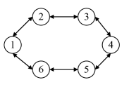
Figure 2: Communication graph $\mathcal{G}$

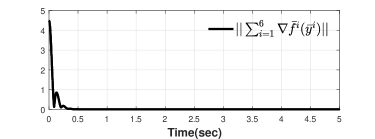
Figure 3: Trajectory of the norm of global objective function, where $\nabla\bar{f}^{i}(\bar{y}^{i})$ denotes the gradient of local objective function in (63).

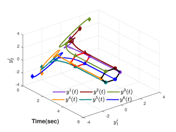
Figure 4: Trajectories of positions $y^{i}$ of the six robots in three-dimensional space for $0\leq t\leq 5s$, where $\blacklozenge$, $\blacktriangle$ and $\bullet$ denote the initial position, position at the prescribed time, and final position, respectively, the red and black regular hexagons represent the formation of the six robots at the prescribed time and final time.

We consider a network composed of six EL agents to cooperatively search for an unknown heat source. Each agent is equipped with sensors to measure gradient information of heat source with respect to distance. The objective is to design controller $u^{i}$ such that the six robots approach the heat source in a formation, and reduce the total displacement of the six robots from their original location. Thus, the global objective function is designed as

$$\min\textstyle{\sum}_{i=1}^{6}\left(s_{1}^{i}\|y^{i}-d^{*}\|^{2}+s_{2}^{i}\|y^{i}-y^{i}(t_{0})\|^{2}\right),$$ (62)

$$\mbox{subject to}\quad y^{i}-y^{j}=\omega^{i}-\omega^{j}$$

where $d^{*}$ denotes the two-dimensional coordinates of the heat source, $\omega^{1}=[1,0]^{\scriptscriptstyle\top}$, $\omega^{2}=[1/2,\sqrt{3}/2]^{\scriptscriptstyle\top}$, $\omega^{3}=[-1/2,\sqrt{3}/2]^{\scriptscriptstyle\top}$, $\omega^{4}=[-1,0]^{\scriptscriptstyle\top}$, $\omega^{5}=[-1/2,-\sqrt{3}/2]^{\scriptscriptstyle\top}$, $\omega^{6}=[1/2,-\sqrt{3}/2]^{\scriptscriptstyle\top}$ represent the formation shape, and $s_{1}^{i}$ and $s_{2}^{i}$ are objective weights.

By defining $\bar{y}^{i}=y^{i}-\omega^{i}$, the optimization problem (62) is transformed into

$$\min\textstyle{\sum}_{i=1}^{6}\left(s_{1}^{i}\|\bar{y}^{i}+\omega^{i}-d^{*}\|^{2}+s_{2}^{i}\|\bar{y}^{i}+\omega^{i}-y^{i}(t_{0})\|^{2}\right),$$ (63)

$$\mbox{subject to}\quad\bar{y}^{i}=\bar{y}^{j}$$

which is consistent with (2). For optimization problem (63), we design $\varpi^{i}$- and $v^{i}$-dynamics as in the form of (13), (14) and (15) such that $\varpi^{i}$ converges to optimal solution with the prescribed time and remains at the optimal solution thereafter. Then, the reference trajectory of each robot’s dynamics is changed as

$$\varpi^{i,^{\prime}}=\varpi^{i}+\omega^{i}.$$

Replacing $\varpi^{i}$ in (16)-(21) with $\varpi^{i,^{\prime}}$, the proposed algorithm can solve optimization problem (62). Let the initial condition be $y^{1}(t_{0})=[1,1]^{\scriptscriptstyle\top}$, $y^{2}(t_{0})=[2,2]^{\scriptscriptstyle\top}$, $y^{3}(t_{0})=[3,3]^{\scriptscriptstyle\top}$, $y^{4}(t_{0})=[-2,-3]^{\scriptscriptstyle\top}$, $y^{5}(t_{0})=[-2,-2]^{\scriptscriptstyle\top}$, $y^{6}(t_{0})=[-3,-3]$, $\dot{q}^{i}(t_{0})=[0,0]^{\scriptscriptstyle\top}$, $\varpi^{i}(t_{0})=y^{i}(t_{0})$, $v^{i}(t_{0})=[0,0]^{\scriptscriptstyle\top}$, $\hat{\theta}^{i}(t_{0})=[2,2,2]^{\scriptscriptstyle\top}$ for $i=1,\cdots,6$. The initial time $t_{0}$ is set to $t_{0}=0$, the prescribed-time scale $T=2s$ and total simulation time is $5s$. The parameters and gain function are chosen as $c=1.3$, $\iota=2.44$, $k_{1}^{i}=5$, $k_{2}^{i}=30$, $\sigma^{i}=4$ for $i=1,\cdots,6$, $\mu=10/(T+t_{0}-t)$. The weight coefficients $s_{1}^{i}$ and $s_{2}^{i}$ for objective function (62) are chosen as $s_{1}^{i}=1$ and $s_{2}^{i}=1$ for $i=1,\cdots,6$. The coordinate of the heat source is set as $d^{*}=[0,0]^{\scriptscriptstyle\top}$. The real value of unknown parameters in $M^{i}(q^{i})$ are $p_{1}^{i}=1.301{\rm kg\cdot m^{2}}$, $p_{2}^{i}=0.056{\rm kg\cdot m^{2}}$ and $p_{3}^{i}=0.296{\rm kg\cdot m^{2}}$ for $i=1,\cdots,6$. The fourth-order Runge-Kutta method is used to solve the ordinary differential equations, and the sampling time is $10^{-5}s$.

The simulation results are shown in Fig. 3 and Fig. 4. Fig. 3 demonstrates that $\bar{y}^{i}$ converges to the optimal solution of the optimization problem (63) within a prescribed time and remains at the optimal solution for $i=1,\cdots,6$, which further implies the optimization problem (62) is solved within the given time frame. In Fig. 4, the six robots approach the heat source in formation within a prescribed time and maintain formation subsequently.

7 Conclusion

In this paper, we propose a novel DPTCO algorithm for a class of NELSs. The position of each robot in the network achieves prescribed-time convergence towards the optimal solution within a prescribed time and remains at the optimal solution afterwards. The optimal solution search is in a feedback loop in which position-dependent measured gradient value is used to construct the auxiliary systems. A prescribed-time small-gain criterion is proposed to characterize the interconnected error system and is also used to guide the selection of control parameters. As a future work, it would be intriguing to further consider the DPTCO where the local objective functions subject to bound, equality, and inequality constraints.

Appendix A Proof of Lemma 4.1

Due to (36), $e_{r}$ satisfies

$$\|e_{r}\|\leq\mu^{-\iota}\|\tilde{e}_{r}\|\leq\mu^{-\iota}\|\tilde{e}_{r}\|_{\mathcal{T}}.$$ (64)

Thus the first inequality in (41) holds with $\gamma_{r}(s)=s$. The $\tilde{e}_{s}$ in (36) can be rewritten in a detailed form as

$$\tilde{e}_{s}=\left[\begin{array}[]{c}\mu^{\iota}e_{y}\\ \mu^{\iota-1}\left(\dot{q}+\mu\bar{K}_{1}e_{y}\right)\end{array}\right].$$ (65)

Then one has

$$\|e_{y}\|\leq\mu^{-\iota}\|\tilde{e}_{s}\|_{\mathcal{T}}$$ (66)

where we used $\mu^{\iota}\|e_{y}\|\leq\|\tilde{e}_{s}\|\leq\|\tilde{e}_{s}\|_{\mathcal{T}}$. According to (65) and (66), $\dot{q}$ satisfies

$$\|\dot{q}\| \leq\mu^{1-\iota}\|\tilde{e}_{s}\|+\mu\|\bar{K}_{1}\|\|e_{y}\|$$

$$\leq\mu^{1-\iota}\|\tilde{e}_{s}\|_{\mathcal{T}}+\|\bar{K}_{1}\|\mu^{1-\iota}\|\tilde{e}_{s}\|_{\mathcal{T}}$$

$$\leq(1+\|\bar{K}_{1}\|)\mu^{1-\iota}\|\tilde{e}_{s}\|_{\mathcal{T}}.$$ (67)

By (66) and (67), the second inequality in (41) holds with $\gamma_{s}(s)=(1+\|\bar{K}_{1}\|+b^{-1})s$ where we used $\mu^{-1}(t)\leq\mu^{-1}(t_{0})=b^{-1}$. By (35) and (41), the upper bound of $\dot{e}_{r}$ is

$$\|\dot{e}_{r}\|\leq\mu^{-\iota+2}\gamma_{e}(\|\tilde{e}\|_{\mathcal{T}})$$ (68)

where $\tilde{e}=\left[\tilde{e}_{r}^{\scriptscriptstyle\top},\tilde{e}_{s}\right]^{\scriptscriptstyle\top}$ and $\gamma_{e}$ is a $\mathcal{K}_{\infty}$ function denoted as $\gamma_{e}(s)=c(2\lambda_{N}+\varrho_{c}+1)(b^{-1}\gamma_{r}(s)+\gamma_{s}(s))$. Since $\iota>2$, (68) means that $\dot{\varpi}^{i}$ and $\dot{v}^{i}$ are uniformly bounded if $\tilde{e}_{r}$ and $\tilde{e}_{s}$ are uniformly bounded.

Define $z_{j}=[(z_{j}^{1})^{\scriptscriptstyle\top},\cdots,(z_{j}^{N})^{\scriptscriptstyle\top}]^{\scriptscriptstyle\top}$, where $z_{j}^{i}$ is given by (18) and (19) for $j=1,2$ and $i=1,\cdots,N$. Based on (8), (66) and (67), the upper bound of $z_{j}$

$$\|z_{j}\|\leq\mu^{2-\iota}\gamma_{z,j}(\|\tilde{e}_{s}\|_{\mathcal{T}}),\quad j=1,2$$

where $\gamma_{z,1}(s)=(\tilde{b}(\iota-1)+\|\bar{K}_{1}\|)(1+\|\bar{K}_{1}\|)s+\iota\tilde{b}\|\bar{K}_{1}\|s$, $\gamma_{z,2}(s)=\|\bar{K}_{1}\|b^{-1}s$. By Property 2.2, let $\omega^{i}=[(\dot{q}^{i})^{\scriptscriptstyle\top},(z_{1}^{i})^{\scriptscriptstyle\top},(z_{2}^{i})^{\scriptscriptstyle\top}]^{\scriptscriptstyle\top}$, $\Omega(q,\dot{q},z_{1},z_{2})$ satisfies

$$\|\Omega(q,\dot{q},z_{1},z_{2})\|\leq\mu^{-\iota+2}\gamma_{\Omega}(\|\tilde{e}_{s}\|_{\mathcal{T}})$$ (69)

with

$$\gamma_{\Omega}(s) =N\bar{\rho}\big{(}b^{-1}\gamma_{s}(s)+b^{-\iota}(\gamma_{s}(s))^{2}+\textstyle{\sum}_{j=1}^{2}\gamma_{z,j}(s)\big{)}$$

$$\quad+N\bar{\rho}\textstyle{\sum}_{j=1}^{2}b^{-\iota+2}(\gamma_{z,j}(s))^{2}$$

where $\bar{\rho}=\max\{\rho^{1},\cdots,\rho^{N}\}$ with $\rho^{i}$ been denoted in Property 2.2 and we used $\left(\textstyle{\sum}_{i=1}^{n}|x^{i}|\right)^{p}\leq\textstyle{\sum}_{i=1}^{n}\left(|x^{i}|\right)^{p}$ for $x^{i}\in\mathbb{R}$, $0<p\leq 1$ and $i=1,\cdots,n$. By (65) and (69), the upper bound of $\varsigma=\left[(\varsigma^{1})^{\scriptscriptstyle\top},\cdots,(\varsigma^{N})^{\scriptscriptstyle\top}\right]^{\scriptscriptstyle\top}$ with $\varsigma^{i}$ denoted in (21) is

$$\|\varsigma(q,\dot{q},\varpi,\mu)\|\leq\mu\gamma_{\varsigma}(\|\tilde{e}_{s}\|_{\mathcal{T}})$$ (70)

where $\gamma_{\varsigma}(s)=2s\gamma_{\Omega}(s)$. Define the Lyapunov function candidate for $\hat{\theta}$-dynamics as $U(\hat{\theta})=\hat{\theta}^{\scriptscriptstyle\top}\hat{\theta}/2$, then its time derivative along trajectory of (20) is

$$\dot{U}(\hat{\theta}) =-\mu\hat{\theta}^{\scriptscriptstyle\top}\bar{\sigma}\hat{\theta}+\hat{\theta}^{\scriptscriptstyle\top}\varsigma(q,\dot{q},\varpi,\mu)$$

$$\leq-\sigma_{\min}\mu U(\hat{\theta})+(2\sigma_{\min})^{-1}\mu(\gamma_{\varsigma}(\|\tilde{e}_{s}\|_{\mathcal{T}}))^{2}$$ (71)

where

$$\sigma_{\min}=\min\{\sigma^{1},\cdots,\sigma^{N}\}$$ (72)

and we used the fact $\hat{\theta}^{\scriptscriptstyle\top}\varsigma(q,\dot{q},\varpi,\mu)\leq\mu\|\hat{\theta}\|\gamma_{\varsigma}(\|\tilde{e}_{s}\|_{\mathcal{T}})\leq\sigma_{\min}\mu\|\hat{\theta}\|^{2}/2+\mu(\gamma_{\varsigma}(\|\tilde{e}_{s}\|_{\mathcal{T}}))^{2}/(2\sigma_{\min})$. Invoking comparison lemma for (71) yields

$$U(\hat{\theta}) \leq\kappa^{-\sigma_{\min}}(\mu)U(\hat{\theta}(t_{0}))$$

$$\quad+\frac{1}{2\sigma_{\min}^{2}}(\gamma_{\varsigma}(\|\tilde{e}_{s}\|_{\mathcal{T}}))^{2}\left(1-\kappa^{-\sigma_{\min}}(\mu)\right)$$

where $\kappa^{-\sigma_{\min}}(\mu)$ is defined as in (9) with $\alpha(s)=s$. Therefore, the upper bound of $\hat{\theta}$ is

$$\|\hat{\theta}\|\leq\|\hat{\theta}(t_{0})\|+\sigma_{\min}^{-1}\gamma_{\varsigma}(\|\tilde{e}_{s}\|_{\mathcal{T}}).$$ (73)

By (65), (69) and (73), $\pi(q,\dot{q},\varpi,\hat{\theta},\mu)$ satisfies

$$\|\pi(q,\dot{q},\varpi,\hat{\theta},\mu)\|\leq\mu^{-\iota+2}\gamma_{\pi}(\|\tilde{e}_{s}\|_{\mathcal{T}})$$ (74)

where $\gamma_{\pi}(s)=\|\bar{K}_{2}\|s+\gamma_{\Omega}(s)(\|\hat{\theta}(t_{0})\|+\sigma_{\min}^{-1}\gamma_{\varsigma}(s))$ with $\bar{K}_{2}=\mbox{diag}\{k_{2}^{1},\cdots,k_{2}^{N}\}\otimes I_{n}$.

Finally, we prove the boundedness of $\hat{\theta}^{i}$-dynamics for $i\in\mathcal{V}$. Since (20) is a non-homogeneous linear differential equation, we can have an analytic solution of $\hat{\theta}(t)$. Substituting it into (20) yields

$$\dot{\hat{\theta}}(t) =-\mu\bar{\sigma}\kappa^{-\bar{\sigma}}(\mu)\hat{\theta}(t_{0})+\varsigma(t)$$

$$\quad-\mu\bar{\sigma}\kappa^{-\bar{\sigma}}(\mu)\textstyle{\int}_{t_{0}}^{t}\kappa^{\bar{\sigma}}(\mu(\tau))\varsigma(\tau)\mathrm{d}\tau$$ (75)

where $\varsigma(q(t),\dot{q}(t),\varpi(t),\mu)$ is simplified as $\varsigma(t)$, and $\kappa^{-\bar{\sigma}}(\mu)=\exp\left(-\textstyle{\int}_{t_{0}}^{t}\mu(\tau)\bar{\sigma}\mathrm{d}\tau\right)$ and $\kappa^{\bar{\sigma}}(\mu(\tau))=\exp\left(\textstyle{\int}_{t_{0}}^{\tau}\mu(s)\bar{\sigma}\mathrm{d}s\right)$ are diagonal matrix functions. Since $\sigma^{i}\geq\tilde{b}$ for $i\in\mathcal{V}$, one has $\sigma_{\min}\geq\tilde{b}$. Let $\sigma_{\max}=\max\{\sigma^{1},\cdots,\sigma^{N}\}$, then

$$\|\mu\bar{\sigma}\kappa^{-\bar{\sigma}}(\mu)\hat{\theta}(t_{0})\|$$

$$\leq\sigma_{\max}\|\hat{\theta}(t_{0})\|\mu\kappa^{-\sigma_{\min}}(\mu)$$

$$\leq\sigma_{\max}\|\hat{\theta}(t_{0})\|b\exp\left(\textstyle{\int}_{t_{0}}^{t}\dot{\mu}(\tau)/\mu(\tau)\mathrm{d}\tau\right)\kappa^{-\sigma_{\min}}(\mu)$$

$$\leq\sigma_{\max}\mu(t_{0})\|\hat{\theta}(t_{0})\|\kappa^{(\tilde{b}-\sigma_{\min})}(\mu)$$

$$\leq\sigma_{\max}\mu(t_{0})\|\hat{\theta}(t_{0})\|$$ (76)

holds for $t\in\mathcal{T}_{p}$. According to the definition of $\mu(t)$ in Definition 2.1, we have $(\mu(t))^{-1}:\mathcal{T}_{p}\mapsto(0,b^{-1}]$ being strictly decreasing to zero. By the definition of a left limit, for any given $\varepsilon>0$ (no matter how small), there always exists $\delta>0$ such that for $0<T+t_{0}-t<\delta$, it holds that $(\mu(t))^{-1}<\varepsilon$. Thus for any pair $(\varepsilon,\delta)$, it follows that $\mu(t)<\infty$ for $t\in[t_{0},T+t_{0}-\delta]$ and $\mu(t)=\infty$ for $t\in(T+t_{0}-\delta,T+t_{0})$. Referring to (70), we observe that $\varsigma(t)$ and consequently $\mu\bar{\sigma}\kappa^{-\bar{\sigma}}(\mu)\textstyle{\int}_{t_{0}}^{t}\kappa^{\bar{\sigma}}(\mu(\tau))\varsigma(\tau)\mathrm{d}\tau$ are bounded for $t\in[t_{0},T+t_{0}-\delta)$. Therefore, combining this with (76), we conclude that $\dot{\hat{\theta}}$ is bounded for $t\in[t_{0},T+t_{0}-\delta)$. As for $t\in(T+t_{0}-\delta,T+t_{0})$, by arithmetic operations of ultimate limit and L’Hospital’s rule,

$$\lim_{t\to T+t_{0}}\left(\varsigma(t)-\mu\bar{\sigma}\kappa^{-\bar{\sigma}}(\mu)\textstyle{\int}_{t_{0}}^{t}\kappa^{\bar{\sigma}}(\mu(\tau))\varsigma(\tau)\mathrm{d}\tau\right)$$

$$=\lim_{t\to T+t_{0}}\varsigma(t)-\lim_{t\to T+t_{0}}\mu(t)\bar{\sigma}$$

$$\quad\times\lim_{t\to T+t_{0}}\kappa^{-\bar{\sigma}}(\mu(t))\textstyle{\int}_{t_{0}}^{t}\kappa^{\bar{\sigma}}(\mu(\tau))\varsigma(\tau)\mathrm{d}\tau$$

$$=\lim_{t\to T+t_{0}}\varsigma(t)-\lim_{t\to T+t_{0}}\mu\bar{\sigma}\kappa^{\bar{\sigma}}(\mu)\varsigma(t)/(\mu\kappa^{\bar{\sigma}}(\mu)\bar{\sigma})$$

$$=\lim_{t\to T+t_{0}}\varsigma(t)-\lim_{t\to T+t_{0}}\varsigma(t)=0.$$

Thus, $\dot{\hat{\theta}}(t)$ is bounded for $t\in\mathcal{T}_{p}$. This completes the proof.

Appendix B Proof of Theorem 4.1

According to (43) and (44), one has

$$\begin{gathered}\underline{\alpha}_{1}(\|\chi_{1}\|)\leq V_{1}(\chi_{1})\leq\overline{\alpha}_{1}(\|\chi_{1}\|),\\ \dot{V}_{1}\leq-\alpha_{1}(\mu)V_{1}+l_{1}\alpha_{2}(\mu)V_{2}(\chi_{2})+\gamma_{1}(\mu)\epsilon_{1}(\|d_{1}\|),\end{gathered}$$

$$\begin{gathered}\underline{\alpha}_{2}(\|\chi_{2}\|)\leq V_{2}(\chi_{2})\leq\overline{\alpha}_{2}(\|\chi_{2}\|),\\ \dot{V}_{2}\leq-\alpha_{2}(\mu)V_{2}+l_{2}\alpha_{1}(\mu)V_{1}(\chi_{1})+\gamma_{2}(\mu)\epsilon_{2}(\|d_{2}\|).\end{gathered}$$

Since $l_{1}l_{2}<1$, by some simple algebra operations, one has

$$l_{1}l_{2}<\sqrt{l_{1}l_{2}}<1.$$

Define the Lyapunov function candidate for $\chi$-dynamics as

$$V(\chi)=l_{2}V_{1}(\chi_{1})+\sqrt{l_{1}l_{2}}V_{2}(\chi_{2}).$$ (77)

Then the time derivative along the trajectories of (43) and (44) is

$$\dot{V} (\chi)\leq l_{2}(-\alpha_{1}(\mu)V_{1}+l_{1}\alpha_{2}(\mu)V_{2}+\gamma_{1}(\mu)\epsilon_{1}(\|d_{1}\|))$$

$$\quad+\sqrt{l_{1}l_{2}}(-\alpha_{2}(\mu)V_{2}+l_{2}\alpha_{1}(\mu)V_{1}+\gamma_{2}(\mu)\epsilon_{2}(\|d_{2}\|))$$

$$=-\left(1-\sqrt{l_{1}l_{2}}\right)\left(l_{2}\alpha_{1}(\mu)V_{1}(\chi_{1})+\sqrt{l_{1}l_{2}}\alpha_{2}(\mu)V_{2}(\chi_{2})\right)$$

$$\quad+l_{2}\gamma_{1}(\mu)\epsilon_{1}(\|d_{1}\|)+\sqrt{l_{1}l_{2}}\gamma_{2}(\mu)\epsilon_{2}(\|d_{2}\|)$$

$$\leq-\left(1-\sqrt{l_{1}l_{2}}\right)\min\{\alpha_{1}(\mu),\alpha_{2}(\mu)\}V(\chi)$$

$$\quad+\max\{\gamma_{1}(\mu),\gamma_{2}(\mu)\}\left(l_{2}\epsilon_{1}(\|d_{1}\|)+\sqrt{l_{1}l_{2}}\epsilon_{2}(\|d_{2}\|)\right)$$

$$\leq-\alpha(\mu)V(\chi)+\gamma(\mu)\epsilon(\|d\|)$$ (78)

with

$$\begin{gathered}\alpha(\mu)=\left(1-\sqrt{l_{1}l_{2}}\right)\min\{\alpha_{1}(\mu),\alpha_{2}(\mu)\},\\ \gamma(\mu)=\gamma_{1}(\mu)+\gamma_{2}(\mu),\\ \epsilon(\|d\|)=l_{2}\epsilon_{1}(\|d\|)+\sqrt{l_{1}l_{2}}\epsilon_{2}(\|d\|)\end{gathered}$$

where $\alpha$, $\gamma$, $\epsilon\in\mathcal{K}_{\infty}$, $d=[d_{1}^{\scriptscriptstyle\top},d_{2}^{\scriptscriptstyle\top}]^{\scriptscriptstyle\top}$, and we used the fact $\|d_{i}\|\leq\|d\|$ for $i=1,2$. We note that $\alpha(\mu)$ may be piecewise continuous but is integrable. Since $d_{i}$ belongs to a compact set $\mathbb{D}_{i}$, by (46), there exists a $\mathcal{K}_{\infty}$ function $\tilde{\epsilon}$ such that

$$\frac{\gamma(\mu)\epsilon(\|d\|)}{\alpha(\mu)}\leq \left(\sup_{\mu\in\mathbb{R}_{p}}\frac{\gamma(\mu)}{\alpha(\mu)}\right)\epsilon(\|d\|_{\mathcal{T}})=\tilde{\epsilon}(\|d\|_{\mathcal{T}})<\infty,$$

where $\|d\|_{\mathcal{T}}=\sup_{t\in\mathcal{T}_{p}}\|d(t)\|$. Invoking comparison lemma for (78) yields

$$V(\chi) \leq\kappa^{-1}(\alpha(\mu))V(\chi_{0})+\int_{t_{0}}^{t}\exp\left(-\textstyle{\int}_{\tau}^{t}\alpha(\mu(s))\mathrm{d}s\right)$$

$$\quad\times\gamma(\mu(\tau))\epsilon(\|d(\tau)\|)\mathrm{d}\tau$$

$$=\kappa^{-1}(\alpha(\mu))V(\chi_{0})+\kappa^{-1}(\alpha(\mu))\int_{t_{0}}^{t}\kappa(\alpha(\mu(\tau)))$$

$$\quad\times\gamma(\mu(\tau))\epsilon(\|d(\tau)\|)\mathrm{d}\tau$$

$$\leq\kappa^{-1}(\alpha(\mu))V(\chi_{0})+\tilde{\epsilon}(\|d\|_{\mathcal{T}})\kappa^{-1}(\alpha(\mu))$$

$$\quad\times\int_{t_{0}}^{t}\kappa(\alpha(\mu(\tau)))\alpha(\mu(\tau))\mathrm{d}\tau$$

$$=\kappa^{-1}(\alpha(\mu))V(\chi_{0})+\tilde{\epsilon}(\|d\|_{\mathcal{T}})\kappa^{-1}(\alpha(\mu))$$

$$\quad\times\int_{0}^{\int_{t_{0}}^{t}\alpha(\mu(s))\mathrm{d}s}\kappa(\alpha(\mu(\tau)))\mathrm{d}\left(\textstyle{\int}_{t_{0}}^{\tau}\alpha(\mu(s))\mathrm{d}s\right)$$

$$=\kappa^{-1}(\alpha(\mu))V(\chi_{0})+\tilde{\epsilon}(\|d\|_{\mathcal{T}})(1-\kappa^{-1}(\alpha(\mu))).$$ (79)

By (43), (44) and (79), for $i=1,2$, $\|\chi_{i}\|$ satisfies

$$\|\chi_{i}\|\leq\underline{\alpha}_{i}^{-1}\circ\overline{\alpha}(\|\chi(t_{0})\|)$$

where $\overline{\alpha}(s)\in\mathcal{K}_{\infty}^{e}$ denoted as

$$\overline{\alpha}(s) =\max\{l_{2}^{-1},(l_{1}l_{2})^{-1/2}\}\big{(}\tilde{\epsilon}(\|d\|_{\mathcal{T}})$$

$$\quad+\max\{l_{2},\sqrt{l_{1}l_{2}}\}\left(\overline{\alpha}_{1}(s)+\overline{\alpha}_{2}(s)\right)\big{)}.$$ (80)

Upon using the fact that $\left(\textstyle{\sum}_{i=1}^{n}|x_{i}|\right)^{p}\leq\textstyle{\sum}_{i=1}^{n}|x_{i}|^{p}$ for $x_{i}\in\mathbb{R},i=1,\cdots,n$, $0<p\leq 1$, we then have

$$\|\chi\| =\sqrt{\chi_{1}^{\scriptscriptstyle\top}\chi_{1}+\chi_{2}^{\scriptscriptstyle\top}\chi_{2}}\leq\|\chi_{1}\|+\|\chi_{2}\|$$

$$\leq\textstyle{\sum}_{i=1}^{2}\underline{\alpha}_{i}^{-1}\circ\overline{\alpha}(\|\chi(t_{0})\|).$$ (81)

Therefore, (81) leads to (47) with $\tilde{\alpha}$ denoted as

$$\tilde{\alpha}(s)=\textstyle{\sum}_{i=1}^{2}\underline{\alpha}_{i}^{-1}\circ\overline{\alpha}(s).$$

This completes the proof.

Appendix C Proof of Lemma 5.1

Define $\bar{R}=[r_{1},r_{2}]\otimes I_{n}\in\mathbb{R}^{nN\times nN}$ an orthogonal matrix with $r_{1}\in\mathbb{R}^{N}$ and $r_{2}\in\mathbb{R}^{N\times N-1}$ satisfy $r_{1}=1_{N}/\sqrt{N}$, $r_{1}^{\scriptscriptstyle\top}r_{2}=0$, $r_{2}^{\scriptscriptstyle\top}r_{2}=I_{N-1}$ and $r_{2}r_{2}^{\scriptscriptstyle\top}=\Pi_{N}$, where $\Pi_{N}=I_{N}-\frac{1}{N}1_{N}1_{N}^{\scriptscriptstyle\top}$. We introduce the following state transformations

$$\xi=\mu^{\iota}\bar{R}^{\scriptscriptstyle\top}e_{\varpi},\quad\psi=\mu^{\iota}\bar{R}^{\scriptscriptstyle\top}e_{v},\quad\phi=\mu^{\iota}\bar{R}^{\scriptscriptstyle\top}e_{y}$$ (82)

where $\xi=[\xi_{1}^{\scriptscriptstyle\top},\xi_{2}^{\scriptscriptstyle\top}]^{\scriptscriptstyle\top}$, $\psi=[\psi_{1}^{\scriptscriptstyle\top},\psi_{2}^{\scriptscriptstyle\top}]^{\scriptscriptstyle\top}$ and $\phi=[\phi_{1}^{\scriptscriptstyle\top},\phi_{2}^{\scriptscriptstyle\top}]^{\scriptscriptstyle\top}$ with $\xi_{1},\psi_{1},\phi_{1}\in\mathbb{R}^{n}$ and $\xi_{2},\psi_{2},\phi_{2}\in\mathbb{R}^{(N-1)n}$. By (13) and (14), for $t\in\mathcal{T}_{p}$, we have the following derivatives

$$\dot{\xi}_{1} = -c\mu^{\iota+1}\bar{r}_{1}^{\scriptscriptstyle\top}\big{(}\nabla\tilde{F}(\varpi,\varpi^{*})+\nabla\tilde{F}(y,\varpi)\big{)}+\iota\tilde{\mu}\xi_{1},$$ (83)

$$\dot{\xi}_{2} = -c\mu^{\iota+1}\bar{r}_{2}^{\scriptscriptstyle\top}\big{(}\nabla\tilde{F}(\varpi,\varpi^{*})+\nabla\tilde{F}(y,\varpi)\big{)}-c\mu\psi_{2}$$ (84)

$$\quad-c\mu\bar{\mathcal{L}}_{r}\left(\xi_{2}+\phi_{2}\right)+\iota\tilde{\mu}\xi_{2},$$

$$\dot{\psi}_{1} = 0,\quad\dot{\psi}_{2}=c\mu\bar{\mathcal{L}}_{r}(\xi_{2}+\phi_{2})+\iota\tilde{\mu}\psi_{2}$$ (85)

where $\bar{r}_{1}=r_{1}\otimes I_{n}$, $\bar{r}_{2}=r_{2}\otimes I_{n}$, $\bar{\mathcal{L}}_{r}=r_{2}^{\scriptscriptstyle\top}\mathcal{L}r_{2}\otimes I_{n}$ and $\tilde{\mu}=\dot{\mu}/\mu$. Define the Lyapunov function candidate for $\xi$- and $\psi$-dynamics as $V(\xi,\psi)=V_{1}(\xi,\psi)+V_{2}(\xi,\psi)$ with

$$\begin{gathered}V_{1}(\xi,\psi)=\frac{\delta}{2}(\xi^{\scriptscriptstyle\top}\xi+\psi^{\scriptscriptstyle\top}\tilde{\mathcal{L}}_{r}^{-1}\psi),\\ V_{2}(\xi,\psi)=(\xi+\psi)^{\scriptscriptstyle\top}(\xi+\psi)\end{gathered}$$ (88)

where $\delta$ is denoted in (52), and $\tilde{\mathcal{L}}_{r}=\mbox{diag}\{I_{n},\bar{\mathcal{L}}_{r}\}\in\mathbb{R}^{nN\times nN}$ is a positive definite matrix. By (83), (84) and (85), the time derivative of $V_{1}(\xi,\psi)$ is

$$\dot{V}_{1}(\xi,\psi)$$

$$=\delta(\xi_{1}^{\scriptscriptstyle\top}\dot{\xi}_{1}+\xi_{2}^{\scriptscriptstyle\top}\dot{\xi}_{2}+\psi_{2}^{\scriptscriptstyle\top}\bar{\mathcal{L}}_{r}^{-1}\dot{\psi}_{2})$$

$$=\delta\iota\tilde{\mu}\left(\|\xi\|^{2}+\psi_{2}^{\scriptscriptstyle\top}\bar{\mathcal{L}}_{r}^{-1}\psi_{2}\right)+\delta c\mu^{\iota+1}\big{(}-\xi_{1}^{\scriptscriptstyle\top}\bar{r}_{1}^{\scriptscriptstyle\top}\nabla\tilde{F}(\varpi,\varpi^{*})$$

$$\quad-\xi_{1}^{\scriptscriptstyle\top}\bar{r}_{1}^{\scriptscriptstyle\top}\nabla\tilde{F}(y,\varpi)-\xi_{2}^{\scriptscriptstyle\top}\bar{r}_{2}^{\scriptscriptstyle\top}\nabla\tilde{F}(\varpi,\varpi^{*})-\xi_{2}^{\scriptscriptstyle\top}\bar{r}_{2}^{\scriptscriptstyle\top}\nabla\tilde{F}(y,\varpi)\big{)}$$

$$\quad+\delta c\mu\left(-\xi_{2}^{\scriptscriptstyle\top}\bar{\mathcal{L}}_{r}\xi_{2}-\xi_{2}^{\scriptscriptstyle\top}\bar{\mathcal{L}}_{r}\phi_{2}+\psi_{2}^{\scriptscriptstyle\top}\phi_{2}\right)$$ (89)

where we used $\psi_{1}^{\scriptscriptstyle\top}\dot{\psi}_{1}=0$. Upon using (8), Young’s inequality, and Assumption 2.3, a few facts are $\tilde{\mu}\big{(}\|\xi\|^{2}+\psi_{2}^{\scriptscriptstyle\top}\bar{\mathcal{L}}_{r}^{-1}\psi_{2}\big{)}\leq\tilde{b}\mu\big{(}\|\xi\|^{2}+\lambda_{2}^{-1}\|\psi\|^{2}\big{)}$, $-\mu^{\iota}\big{(}\xi_{1}^{\scriptscriptstyle\top}\bar{r}_{1}^{\scriptscriptstyle\top}\nabla\tilde{F}(\varpi,\varpi^{*})+\xi_{2}^{\scriptscriptstyle\top}\bar{r}_{2}^{\scriptscriptstyle\top}\nabla\tilde{F}(\varpi,\varpi^{*})\big{)}\leq-\rho_{c}\|\xi\|^{2}$, $-\mu^{\iota}\big{(}\xi_{1}^{\scriptscriptstyle\top}\bar{r}_{1}^{\scriptscriptstyle\top}\nabla\tilde{F}(y,\varpi)+\xi_{2}^{\scriptscriptstyle\top}\bar{r}_{2}^{\scriptscriptstyle\top}\nabla\tilde{F}(y,\varpi)\big{)}\leq\rho_{c}\|\xi\|^{2}/2+\varrho_{c}^{2}\|\phi\|^{2}/(2\rho_{c})$, $-\xi_{2}^{\scriptscriptstyle\top}\bar{\mathcal{L}}_{r}\phi_{2}\leq\lambda_{2}\|\xi_{2}\|^{2}/2+\lambda_{N}^{2}\|\phi_{2}\|^{2}/(2\lambda_{2})$ and $\psi_{2}^{\scriptscriptstyle\top}\phi_{2}\leq\|\psi_{2}\|^{2}/(8\delta)+2\delta\|\phi_{2}\|^{2}$. Therefore, according to the above inequalities, $\dot{V}_{1}(\xi,\psi)$ satisfies

$$\dot{V}_{1}(\xi,\psi) \leq\big{(}-\rho_{c}c/2+\iota\tilde{b}\big{)}\delta\mu\|\xi\|_{2}-\lambda_{2}c\delta\mu\|\xi_{2}\|^{2}/2$$

$$\quad+\left(\varrho_{c}^{2}/(2\rho_{c})+\lambda_{N}^{2}/(2\lambda_{2})+2\delta\right)c\delta\mu\|\phi\|^{2}$$

$$\quad+\big{(}\iota\tilde{b}/\lambda_{2}+c/(8\delta)\big{)}\delta\mu\|\psi\|^{2}$$ (90)

where we used $\|\phi_{2}\|\leq\|\phi\|$ and $\|\psi_{2}\|\leq\|\psi\|$. The derivative of $V_{2}(\xi,\psi)$ can be expressed as

$$\dot{V}_{2}(\xi,\psi)$$

$$=\xi_{1}^{\scriptscriptstyle\top}\dot{\xi}_{1}+\xi_{2}^{\scriptscriptstyle\top}\dot{\xi}_{2}+\xi_{2}^{\scriptscriptstyle\top}\dot{\psi}_{2}+\psi_{1}^{\scriptscriptstyle\top}\dot{\xi}_{1}+\psi_{2}^{\scriptscriptstyle\top}\dot{\xi}_{2}+\psi_{2}^{\scriptscriptstyle\top}\dot{\psi}_{2}$$

$$=-c\mu^{\iota+1}\left(\xi_{1}^{\scriptscriptstyle\top}\bar{r}_{1}^{\scriptscriptstyle\top}+\xi_{2}^{\scriptscriptstyle\top}\bar{r}_{2}^{\scriptscriptstyle\top}\right)\big{(}\nabla\tilde{F}(\varpi,\varpi^{*})+\nabla\tilde{F}(y,\varpi)\big{)}$$

$$\quad-c\mu^{\iota+1}\left(\psi_{1}^{\scriptscriptstyle\top}\bar{r}_{1}^{\scriptscriptstyle\top}+\psi_{2}^{\scriptscriptstyle\top}\bar{r}_{2}^{\scriptscriptstyle\top}\right)\big{(}\nabla\tilde{F}(\varpi,\varpi^{*})+\nabla\tilde{F}(y,\varpi)\big{)}$$

$$\quad-c\mu\left(\xi_{2}^{\scriptscriptstyle\top}\psi_{2}+\psi_{2}^{\scriptscriptstyle\top}\psi_{2}\right)+\iota\tilde{\mu}\|\xi+\psi\|^{2}.$$

By Young’s inequality and (8), one has $-\mu^{\iota}(\psi_{1}^{\scriptscriptstyle\top}\bar{r}_{1}^{\scriptscriptstyle\top}+\psi_{2}^{\scriptscriptstyle\top}\bar{r}_{2}^{\scriptscriptstyle\top})\nabla\tilde{F}(\varpi,\varpi^{*})\leq\|\psi\|^{2}/8+2\varrho_{c}^{2}\|\xi\|^{2}$, $-\mu^{\iota}(\psi_{1}^{\scriptscriptstyle\top}\bar{r}_{1}^{\scriptscriptstyle\top}+\psi_{2}^{\scriptscriptstyle\top}\bar{r}_{2}^{\scriptscriptstyle\top})\nabla\tilde{F}(y,\varpi)\leq\|\psi\|^{2}/8+2\varrho_{c}^{2}\|\phi\|^{2}$, $-\xi_{2}^{\scriptscriptstyle\top}\psi_{2}\leq 2\|\xi_{2}\|^{2}+\|\psi_{2}\|^{2}/8$ and $\iota\tilde{\mu}\|\xi+\psi\|^{2}\leq 2\iota\tilde{b}\mu\left(\|\xi\|^{2}+\|\psi\|^{2}\right)$. Then by the inequalities under (89), and the upper inequalities, $\dot{V}_{2}(\xi,\psi)$ satisfies

$$\dot{V}_{2}(\xi,\psi)$$

$$\leq\big{(}-\rho_{c}c/2+2c\varrho_{c}^{2}+2\iota\tilde{b}\big{)}\mu\|\xi\|^{2}+\big{(}5c/8+2\iota\tilde{b}\big{)}\mu\|\psi\|^{2}$$

$$\quad+2c\mu\|\xi_{2}\|^{2}+c\left(\varrho_{c}^{2}/(2\rho_{c})+2\varrho_{c}^{2}\right)\mu\|\phi\|^{2}.$$ (91)

Therefore, by (90) and (91), $\dot{V}(\xi,\psi)$ satisfies

$$\dot{V}(\xi,\psi)\leq \big{(}-\rho_{c}c\delta/2-\rho_{c}c/2+2c\varrho_{c}^{2}+\delta\iota\tilde{b}+2\iota\tilde{b}\big{)}\mu\|\xi\|^{2}$$

$$+\big{(}-c/2+\delta\iota\tilde{b}/\lambda_{2}+2\iota\tilde{b}\big{)}\mu\|\psi\|^{2}$$

$$+c_{\Delta}\mu\|\phi\|^{2}+\left(-\delta\lambda_{2}c/2+2c\right)\mu\|\xi_{2}\|^{2}$$

where $c_{\Delta}$ is denoted in (55). Recall the definition of $\delta$ in (52), we have $-\rho_{c}\delta c/2-\rho_{c}c/2+2c\varrho_{c}^{2}\leq-c/2$ and $-\delta\lambda_{2}c/2+2c\leq 0$. Therefore, for $c$ denoted in (53), $\dot{V}(\xi,\psi)$ further satisfies

$$\dot{V}(\xi,\psi)\leq-\bar{\delta}c^{*}\mu\left(\|\xi\|^{2}+\|\psi\|^{2}\right)+c_{\Delta}\mu\|\phi\|^{2}.$$ (92)

We define the Lyapunov functions for $\tilde{e}_{r}$- and $\tilde{e}_{s}^{\prime}$-dynamics as

$$U(\tilde{e}_{r})=\frac{\delta}{2}\tilde{e}_{r}^{\scriptscriptstyle\top}\Lambda_{r,1}\tilde{e}_{r}+\frac{1}{2}\tilde{e}_{r}^{\scriptscriptstyle\top}\Lambda_{r,2}\tilde{e}_{r},$$ (93)

$$W(\tilde{e}_{s}^{\prime})=\left(\tilde{e}_{s}^{\prime}\right)^{\scriptscriptstyle\top}\Lambda_{s}\tilde{e}_{s}^{\prime}$$ (94)

where $\Lambda_{r,1}=\mbox{diag}\{I_{mn},\bar{R}\tilde{\mathcal{L}}_{r}^{-1}\bar{R}^{\scriptscriptstyle\top}\}$, $\Lambda_{r,2}=[I_{mn}\;I_{mn}]^{\scriptscriptstyle\top}[I_{mn}\;I_{mn}]$ and $\Lambda_{s}=\mbox{diag}\{I_{nN},M(q),I_{pN}\}$. We note

$$U(\tilde{e}_{r})=V(\xi,\psi),\quad\dot{U}(\tilde{e}_{r})=\dot{V}(\xi,\psi).$$

We decompose $\tilde{e}_{s}$ in (36) as

$$\tilde{e}_{s}=\left[\tilde{e}_{s,1}^{\scriptscriptstyle\top},\tilde{e}_{s,2}^{\scriptscriptstyle\top}\right]^{\scriptscriptstyle\top}$$

with $\tilde{e}_{s,1}=\mu^{\iota}e_{y}$ and $\tilde{e}_{s,2}=\mu^{\iota-1}\left(\dot{q}+\mu\bar{K}_{1}e_{y}\right)$. Since $\bar{R}$ in (82) is an orthogonal matrix, by (36), one has $\|\phi\|\leq\|\tilde{e}_{s,1}\|$, then according to (92), (93) and the fact $\|\tilde{e}_{s,1}\|^{2}\leq W(\tilde{e}_{s}^{\prime})$,

$$\begin{gathered}\underline{\delta}\|\tilde{e}_{r}\|^{2}\leq U(\tilde{e}_{r})\leq\bar{\delta}\|\tilde{e}_{r}\|^{2},\\ \dot{U}(\tilde{e}_{r})\leq-c^{*}\mu U(\tilde{e}_{r})+c_{\Delta}\mu W(\tilde{e}_{s}^{\prime}).\end{gathered}$$ (95)

Now we prove $\tilde{e}_{s}^{\prime}$-dynamics admits a prescribed-time ISS Lyapunov function. It’s worth noting that $\Lambda_{s}$ in (94) is positive definition according to Property 2.3. Then $2\tilde{e}_{s,1}^{\scriptscriptstyle\top}\dot{\tilde{e}}_{s,1}$ can be expressed as

$$2\tilde{e}_{s,1}^{\scriptscriptstyle\top}\dot{\tilde{e}}_{s,1} =2\tilde{e}_{s,1}^{\scriptscriptstyle\top}(\iota\mu^{\iota-1}\dot{\mu}e_{y}+\mu^{\iota}(\dot{q}-\dot{\varpi}))$$

$$=2\tilde{e}_{s,1}^{\scriptscriptstyle\top}(\iota\tilde{\mu}\tilde{e}_{s,1}+\mu\tilde{e}_{s,2}-\mu\bar{K}_{1}\tilde{e}_{s,1}-\mu^{\iota}\dot{\varpi})$$

where we used $\mu\dot{q}=\mu\tilde{e}_{s,2}-\mu^{\iota+1}\bar{K}_{1}e_{y}$ according to (65). By Young’s inequality, (8) and (56), one has $2\tilde{\mu}\iota\|\tilde{e}_{s,1}\|^{2}\leq 2\tilde{b}\iota\mu\|\tilde{e}_{s,1}\|^{2}$, $2\mu\tilde{e}_{s,1}^{\scriptscriptstyle\top}\tilde{e}_{s,2}\leq\mu\|\tilde{e}_{s,1}\|^{2}+\mu\|\tilde{e}_{s,1}\|^{2}$, $-2\mu^{l}\tilde{e}_{s,1}^{\scriptscriptstyle\top}\dot{\varpi}\leq\mu\|\tilde{e}_{s,1}\|^{2}+\mu^{2\iota-1}\|\dot{\varpi}\|^{2}$ and $-2\mu\tilde{e}_{s,1}^{\scriptscriptstyle\top}\bar{K}_{1}\tilde{e}_{s,1}=-2\mu\tilde{e}_{s,1}^{\scriptscriptstyle\top}\bar{K}_{1}^{*}\tilde{e}_{s,1}-2(\tilde{b}\iota+1)\mu\|\tilde{e}_{s,1}\|^{2}$, where $\bar{K}_{1}^{*}=\mbox{diag}\{k_{1}^{1,*},\cdots,k_{1}^{N,*}\}\otimes I_{n}$. Substituting the above inequalities into $2\tilde{e}_{s}^{\scriptscriptstyle\top}\dot{\tilde{e}}_{s}$ yields

$$2\tilde{e}_{s,1}^{\scriptscriptstyle\top}\dot{\tilde{e}}_{s,1}\leq-2\mu\tilde{e}_{s,1}^{\scriptscriptstyle\top}\bar{K}_{1}^{*}\tilde{e}_{s,1}+\mu\|\tilde{e}_{s,2}\|^{2}+\mu^{2\iota-1}\|\dot{\varpi}\|^{2}.$$ (96)

We note

$$\frac{\mathrm{d}\tilde{e}^{\scriptscriptstyle\top}M(q)\tilde{e}_{s,2}}{\mathrm{d}t}=2\tilde{e}_{s,2}^{\scriptscriptstyle\top}M(q)\dot{\tilde{e}}_{s,2}+\tilde{e}_{s,2}^{\scriptscriptstyle\top}\dot{M}(q)\tilde{e}_{s,2}.$$

According to (1), (16) and (65), one has

$$\tilde{e}_{s,2}^{\scriptscriptstyle\top}M(q)\dot{\tilde{e}}_{s,2}$$

$$=\tilde{e}_{s,2}^{\scriptscriptstyle\top}\Big{[}(\iota-1)\tilde{\mu}M(q)\tilde{e}_{s,2}+\tilde{\mu}M(q)\bar{K}_{1}\tilde{e}_{s,1}$$

$$\quad+\mu^{\iota}M(q)\bar{K}_{1}(\dot{q}-\dot{\varpi})+\mu^{\iota-1}(\pi(q,\dot{q},\varpi,\hat{\theta},\mu)-C(q,\dot{q})\dot{q})\Big{]}$$

$$=\tilde{e}_{s,2}^{\scriptscriptstyle\top}\mu^{\iota-1}\Big{[}\pi(q,\dot{q},\varpi,\hat{\theta},\mu)+M(q)z_{1}+C(q,\dot{q})z_{2}$$

$$\quad-\mu M(q)\bar{K}_{1}\dot{\varpi}\Big{]}-\tilde{e}_{s,2}^{\scriptscriptstyle\top}C(q,\dot{q})\tilde{e}_{s,2}$$ (97)

where $z_{1}$ and $z_{2}$ are defined in (18) and (19), and we used the fact $\dot{q}=\mu^{-\iota+1}\left(\tilde{e}_{s,2}-\bar{K}_{1}\tilde{e}_{s,1}\right)$. Note that $\tilde{e}_{s,2}$ can be decomposed as $\tilde{e}_{s,2}=\left[(\tilde{e}_{s,2}^{1})^{\scriptscriptstyle\top},\cdots,(\tilde{e}_{s,2}^{N})^{\scriptscriptstyle\top}\right]^{\scriptscriptstyle\top}$ with $\tilde{e}_{s,2}^{i}=\mu^{\iota-1}(q^{i}+\mu k_{1}^{i}e_{y}^{i})$ for $i\in\mathcal{V}$. By Young’s inequality, one has

$$-2\mu^{\iota}\tilde{e}_{s,2}^{\scriptscriptstyle\top}M(q)\bar{K}_{1}\dot{\varpi}$$

$$=\textstyle{\sum}_{i=1}^{N}\left[(-2\mu^{\iota})k_{1}^{i}(\tilde{e}_{s,2}^{i})^{\scriptscriptstyle\top}M^{i}(q^{i})\dot{\varpi}^{i}\right]$$

$$\leq\textstyle{\sum}_{i=1}^{N}\left[\mu(k_{1}^{i})^{2}(k_{\overline{m}}^{i})^{2}\|\tilde{e}_{s,2}^{i}\|^{2}+\mu^{2\iota-1}\|\dot{\varpi}^{i}\|^{2}\right]$$

$$=\mu\tilde{e}_{s,2}^{\scriptscriptstyle\top}\bar{K}_{1}^{2}\bar{K}_{\overline{m}}^{2}\tilde{e}_{s,2}+\mu^{2\iota-1}\|\dot{\varpi}\|^{2}$$ (98)

where $\bar{K}_{\overline{m}}=\mbox{diag}\{k_{\overline{m}}^{1},\cdots,k_{\overline{m}}^{N}\}\otimes I_{n}$ and we note that $\bar{K}_{1}^{2}\bar{K}_{\overline{m}}^{2}$ is a positive definite matrix. Taking time derivative of $\tilde{\theta}^{\scriptscriptstyle\top}\tilde{\theta}$ yields

$$\tilde{\theta}^{\scriptscriptstyle\top}\dot{\tilde{\theta}}=-\tilde{\theta}^{\scriptscriptstyle\top}\varsigma(q,\dot{q},\varpi^{i},\mu)+\mu\tilde{\theta}^{\scriptscriptstyle\top}\bar{\sigma}\hat{\theta}$$

where $\varsigma(\cdot)$ is defined in (21). According to Property 2.1 and 2.2, one has $-2\tilde{e}_{s,2}^{\scriptscriptstyle\top}C(q,\dot{q})\tilde{e}_{s,2}+\tilde{e}_{s,2}^{\scriptscriptstyle\top}\dot{M}(q)\tilde{e}_{s,2}=0$ and $M(q)z_{1}+C(q,\dot{q})z_{2}=\Omega(q,\dot{q},z_{1},z_{2})\theta$. Substituting $\pi(q,\dot{q},\varpi,\hat{\theta},\mu)$ in (16) and (98) into (97), we have

$$2\tilde{e}_{s,2}^{\scriptscriptstyle\top}M(q)\dot{\tilde{e}}_{s,2}+\tilde{e}_{s,2}^{\scriptscriptstyle\top}\dot{M}(q)\tilde{e}_{s,2}+2\tilde{\theta}^{\scriptscriptstyle\top}\dot{\tilde{\theta}}$$

$$=-\mu\tilde{e}_{s,2}^{\scriptscriptstyle\top}\left(2\bar{K}_{2}-\bar{K}_{1}\bar{K}_{\bar{m}}\right)\tilde{e}_{s,2}+2\mu\tilde{\theta}^{\scriptscriptstyle\top}\bar{\sigma}\hat{\theta}+\mu^{2\iota-1}\|\dot{\varpi}\|^{2}$$

$$\leq-2\mu\tilde{e}_{s,2}^{\scriptscriptstyle\top}\bar{K}_{2}^{*}\tilde{e}_{s,2}-\mu\|\tilde{e}_{s,2}\|^{2}-\mu\tilde{\theta}^{\scriptscriptstyle\top}\bar{\sigma}\tilde{\theta}$$

$$\quad+\mu\theta^{\scriptscriptstyle\top}\bar{\sigma}\theta+\mu^{2\iota-1}\|\dot{\varpi}\|^{2}$$ (99)

where $\bar{K}_{2}^{*}=\mbox{diag}\{k_{2}^{1,*},\cdots,k_{2}^{N,*}\}\otimes I_{n}$ with $k_{2}^{i,*}$ been denoted in (56) for $i\in\mathcal{V}$. We note

$$\underline{\varepsilon}\|\tilde{e}_{s}^{\prime}\|^{2}\leq W(\tilde{e}_{s}^{\prime})\leq\overline{\varepsilon}\|\tilde{e}_{s}^{\prime}\|^{2},$$

$$\dot{W}(\tilde{e}_{s}^{\prime})=2\tilde{e}_{s,1}^{\scriptscriptstyle\top}\dot{\tilde{e}}_{s,1}+2\tilde{e}_{s,2}^{\scriptscriptstyle\top}M(q)\dot{\tilde{e}}_{s,2}+\tilde{e}_{s,2}^{\scriptscriptstyle\top}\dot{M}(q)\tilde{e}_{s,2}+2\tilde{\theta}^{\scriptscriptstyle\top}\dot{\tilde{\theta}}$$

where $\underline{\varepsilon}$ and $\overline{\varepsilon}$ are denoted in (52). By (35) and the fact $\|\dot{\varpi}\|\leq\|\dot{e}_{r}\|$, one has

$$2\mu^{2\iota-1}\|\dot{\varpi}\|^{2}\leq c_{s}\mu(\|\tilde{e}_{r}\|^{2}+\|\tilde{e}_{s,1}\|^{2})$$

where $c_{s}$ is denoted in (55). Then by (94),(96), and (99), $\dot{W}(\tilde{e}_{s}^{\prime})$ further satisfies

$$\dot{W}(\tilde{e}_{s}^{\prime}) \leq -\tilde{k}_{1}\mu\|\tilde{e}_{s,1}\|^{2}-\tilde{k}_{2}\mu\tilde{e}_{s,2}^{\scriptscriptstyle\top}M(q)\tilde{e}_{s,2}$$ (100)

$$-\sigma_{\min}\mu\|\tilde{\theta}\|^{2}+\sigma_{\max}\mu\|\theta\|^{2}+c_{s}\mu\|\tilde{e}_{r}\|^{2}$$

$$\leq -\tilde{k}\mu W(\tilde{e}_{s}^{\prime})+\sigma_{\max}\mu\|\theta\|^{2}+(c_{s}/\underline{\delta})\mu U(\tilde{e}_{r})$$

where $\tilde{k}_{1}$, $\tilde{k}_{2}$ and $\tilde{k}$ have been denoted under (59), and we used the fact

$$-2\mu\tilde{e}_{s,2}^{\scriptscriptstyle\top}\bar{K}_{2}^{*}\tilde{e}_{s,2} =-2\mu\textstyle{\sum}_{i=1}^{N}k_{2}^{i}(\tilde{e}_{s,2}^{i})^{\scriptscriptstyle\top}\tilde{e}_{s,2}^{i}$$

$$\leq-2\mu\textstyle{\sum}_{i=1}^{N}k_{2}^{i}(k_{\bar{m}}^{i})^{-1}(\tilde{e}_{s,2}^{i})^{\scriptscriptstyle\top}M^{i}(q^{i})\tilde{e}_{s,2}^{i}$$

$$=2\mu\tilde{k}_{2}\tilde{e}_{s,2}^{\scriptscriptstyle\top}M(q)\tilde{e}_{s,2}.$$

Therefore, (95) and (100) lead to (58) and (59). This completes the proof.

References

• Abdessameud, (2018) Abdessameud, A. (2018). Consensus of nonidentical euler–lagrange systems under switching directed graphs. IEEE Transactions on Automatic Control, 64(5):2108–2114.
• Abdessameud et al., (2016) Abdessameud, A., Tayebi, A., and Polushin, I. G. (2016). Leader-follower synchronization of euler-lagrange systems with time-varying leader trajectory and constrained discrete-time communication. IEEE Transactions on Automatic Control, 62(5):2539–2545.
• An and Yang, (2021) An, L. and Yang, G.-H. (2021). Collisions-free distributed optimal coordination for multiple euler-lagrangian systems. IEEE Transactions on Automatic Control, 67(1):460–467.
• Chen and Li, (2018) Chen, G. and Li, Z. (2018). A fixed-time convergent algorithm for distributed convex optimization in multi-agent systems. Automatica, 95:539–543.
• Chen et al., (2021) Chen, G., Yang, Q., Song, Y., and Lewis, F. L. (2021). Fixed-time projection algorithm for distributed constrained optimization on time-varying digraphs. IEEE Transactions on Automatic Control, 67(1):390–397.
• Gong and Han, (2024) Gong, P. and Han, Q.-L. (2024). Distributed fixed-time optimization for second-order nonlinear multiagent systems: State and output feedback designs. IEEE Transactions on Automatic Control, 69(5):3198–3205.
• Huang et al., (2019) Huang, B., Zou, Y., Meng, Z., and Ren, W. (2019). Distributed time-varying convex optimization for a class of nonlinear multiagent systems. IEEE Transactions on Automatic control, 65(2):801–808.
• Huang et al., (2015) Huang, J., Wen, C., Wang, W., and Song, Y.-D. (2015). Adaptive finite-time consensus control of a group of uncertain nonlinear mechanical systems. Automatica, 51:292–301.
• Jiang and Liu, (2018) Jiang, Z.-P. and Liu, T. (2018). Small-gain theory for stability and control of dynamical networks: A survey. Annual Reviews in Control, 46:58–79.
• Kia et al., (2015) Kia, S. S., Cortés, J., and Martínez, S. (2015). Distributed convex optimization via continuous-time coordination algorithms with discrete-time communication. Automatica, 55:254–264.
• Kim et al., (2014) Kim, C.-Y., Song, D., Xu, Y., Yi, J., and Wu, X. (2014). Cooperative search of multiple unknown transient radio sources using multiple paired mobile robots. IEEE Transactions on Robotics, 30(5):1161–1173.
• Li et al., (2018) Li, D., Zhang, W., He, W., Li, C., and Ge, S. S. (2018). Two-layer distributed formation-containment control of multiple euler–lagrange systems by output feedback. IEEE Transactions on Cybernetics, 49(2):675–687.
• Li et al., (2024) Li, H., Liu, T., and Jiang, Z.-P. (2024). A lyapunov-based small-gain theorem for a network of finite-time input-to-state stable systems. IEEE Transactions on Automatic Control, 69(2):1052–1059.
• Lin et al., (2016) Lin, P., Ren, W., and Farrell, J. A. (2016). Distributed continuous-time optimization: nonuniform gradient gains, finite-time convergence, and convex constraint set. IEEE Transactions on Automatic Control, 62(5):2239–2253.
• (15) Liu, H., Zheng, W. X., and Yu, W. (2021a). Continuous-time algorithm based on finite-time consensus for distributed constrained convex optimization. IEEE Transactions on Automatic Control, 67(5):2552–2559.
• (16) Liu, T., Qin, Z., Hong, Y., and Jiang, Z.-P. (2021b). Distributed optimization of nonlinear multiagent systems: A small-gain approach. IEEE Transactions on Automatic Control, 67(2):676–691.
• Lu and Liu, (2019) Lu, M. and Liu, L. (2019). Leader–following consensus of multiple uncertain euler–lagrange systems with unknown dynamic leader. IEEE Transactions on Automatic Control, 64(10):4167–4173.
• Lu et al., (2019) Lu, M., Liu, L., and Feng, G. (2019). Adaptive tracking control of uncertain euler–lagrange systems subject to external disturbances. Automatica, 104:207–219.
• Nedic et al., (2010) Nedic, A., Ozdaglar, A., and Parrilo, P. A. (2010). Constrained consensus and optimization in multi-agent networks. IEEE Transactions on Automatic Control, 55(4):922–938.
• Nuno et al., (2013) Nuno, E., Sarras, I., and Basanez, L. (2013). Consensus in networks of nonidentical euler–lagrange systems using p+ d controllers. IEEE Transactions on Robotics, 29(6):1503–1508.
• Pavlichkov, (2018) Pavlichkov, S. (2018). A finite-time small-gain theorem for infinite networks and its applications. In 2018 IEEE Conference on Decision and Control (CDC), pages 700–705. IEEE.
• Qin et al., (2022) Qin, Z., Jiang, L., Liu, T., and Jiang, Z.-P. (2022). Distributed optimization for uncertain euler–lagrange systems with local and relative measurements. Automatica, 139:110113.
• Qin et al., (2023) Qin, Z., Liu, T., Liu, T., Jiang, Z.-P., and Chai, T. (2023). Distributed feedback optimization of nonlinear uncertain systems subject to inequality constraints. IEEE Transactions on Automatic Control.
• Rahili and Ren, (2016) Rahili, S. and Ren, W. (2016). Distributed continuous-time convex optimization with time-varying cost functions. IEEE Transactions on Automatic Control, 62(4):1590–1605.
• Song et al., (2017) Song, Y., Wang, Y., Holloway, J., and Krstic, M. (2017). Time-varying feedback for regulation of normal-form nonlinear systems in prescribed finite time. Automatica, 83:243–251.
• Tang and Wang, (2020) Tang, Y. and Wang, X. (2020). Optimal output consensus for nonlinear multiagent systems with both static and dynamic uncertainties. IEEE Transactions on Automatic Control, 66(4):1733–1740.
• Viel et al., (2019) Viel, C., Bertrand, S., Kieffer, M., and Piet-Lahanier, H. (2019). Distributed event-triggered control strategies for multi-agent formation stabilization and tracking. Automatica, 106:110–116.
• Viel et al., (2022) Viel, C., Kieffer, M., Piet-Lahanier, H., and Bertrand, S. (2022). Distributed event-triggered formation control for multi-agent systems in presence of packet losses. Automatica, 141:110215.
• Wang and Elia, (2010) Wang, J. and Elia, N. (2010). Control approach to distributed optimization. In 2010 48th Annual Allerton Conference on Communication, Control, and Computing (Allerton), pages 557–561. IEEE.
• (30) Wang, X., Wang, G., and Li, S. (2020a). Distributed finite-time optimization for integrator chain multiagent systems with disturbances. IEEE Transactions on Automatic Control, 65(12):5296–5311.
• (31) Wang, X., Wang, G., and Li, S. (2020b). A distributed fixed-time optimization algorithm for multi-agent systems. Automatica, 122:109289.
• Wu et al., (2022) Wu, C., Fang, H., Zeng, X., Yang, Q., Wei, Y., and Chen, J. (2022). Distributed continuous-time algorithm for time-varying optimization with affine formation constraints. IEEE Transactions on Automatic Control, 68(4):2615–2622.
• Zhang et al., (2017) Zhang, Y., Deng, Z., and Hong, Y. (2017). Distributed optimal coordination for multiple heterogeneous euler–lagrangian systems. Automatica, 79:207–213.
• Zou et al., (2021) Zou, Y., Huang, B., and Meng, Z. (2021). Distributed continuous-time algorithm for constrained optimization of networked euler–lagrange systems. IEEE Transactions on Control of Network Systems, 8(2):1034–1042.
• Zou et al., (2020) Zou, Y., Meng, Z., and Hong, Y. (2020). Adaptive distributed optimization algorithms for euler–lagrange systems. Automatica, 119:109060.