Anomalous diffusion in quantum system driven by heavy-tailed stochastic processes

Abstract

In this paper, we study a stochastically driven non-equilibrium quantum system where the driving protocols consist of hopping and waiting processes. The waiting times between two hopping processes satisfy a heavy-tailed distribution. By calculating the squared width of the wavepackets, our findings demonstrate the emergence of various anomalous transport phenomenons when the system remains unchanged within the heavy-tailed regime, including superdiffusive, subdiffusive, and standard diffusive motion. Only subdiffusion occurs when the system has evolved during the waiting process. All these transport behaviors are accompanied by a breakdown of ergodicity, highlighting the complex dynamics induced by the stochastic driving mechanism.

I introduction

The continuous-time random walk (CTRW) model [Montroll and Weiss, 1965; Weiss, 1994; Klafter and Sokolov, 2011] is a mathematical framework used to describe the dynamic behavior of systems, particularly the diffusion process of particles in complex systems and non-uniform media [Scher and Montroll, 1975; Bouchaud and Georges, 1990; Barkai et al., 2000; Weiss, 2013]. This model applies to multiple fields such as physics [Shlesinger, 1974; Pfister and Scher, 1977; Geisel et al., 1985; Solomon et al., 1993; Ohtsuki and Kawarabayashi, 1997], finance [Mandelbrot, 1963; Masoliver et al., 2003; Scalas, 2006], and many others [Helmstetter and Sornette, 2002; Mega et al., 2003; H$\ddot{\rm{o}}$fling and Franosch, 2013], because it can handle discontinuities in time and space as well as long-range dependencies. The CTRW model incorporates two independent stochastic variables [Scher and Montroll, 1975; Metzler and Klafter, 2000]: jump length $x$ and waiting time $t$, as described by the probability distribution functions (PDFs) $\lambda(x)$ and $\psi(t)$, respectively. They characterize a particle’s waiting time $t$ at its initial position, then followed by a jump of length $x$, after which the process restarts. When the PDFs $\lambda(x)$ and $\psi(t)$ exhibit finite first and second moments, such as $\lambda(x)$ and $\psi(t)$ follow a Poissonian and Gaussian distribution, the motion of system corresponds to normal diffusion [Klafter and Sokolov, 2011]. Conversely, if the waiting time PDF $\psi(t)$ adheres to a power-law distribution with a long tail, such that $\psi(t)\propto 1/t^{(1+\alpha)}$ with $0<\alpha<1$, the first moment, $\langle\tau\rangle=\int_{0}^{\infty}t\psi(t)dt$, diverges. The ensemble-averaged mean squared displacements satisfy $\langle x^{2}(t)\rangle_{ens}\sim t^{\alpha}$, indicating a subdiffusive motion [Metzler and Klafter, 2000; Sokolov et al., 2002]. Additionally, the ensemble-averaged mean squared displacements do not equal the time-averaged mean squared displacements, indicating ergodicity breaking [Bouchaud, 1992; Barkai and Margolin, 2004; Margolin and Barkai, 2005; Lubelski et al., 2008; He et al., 2008].

A profusion of equilibrium quantum systems, including generic one-dimensional integrable models  [Zotos et al., 1997; Batchelor, 2005; Miller et al., 2020], chaotic systems [Karrasch et al., 2014; $\rm{\check{Z}nidari\check{c}}$ et al., 2016; Blake et al., 2017; Friedman et al., 2020] or disordered models [Anderson, 1958; Agarwal et al., 2015; Bar Lev et al., 2015; Luitz et al., 2016] typically exhibit ballistic, diffusive or subdiffusive (localization) motion. The dynamics of non-equilibrium have garnered significant interest due to substantial experimental progress [Bloch et al., 2008; Chang et al., 2018]. By employing methods such as quenching [Polkovnikov et al., 2011; Luca D’Alessio and Rigol, 2016], driving [Struck et al., 2012; Cai et al., 2017; Harper et al., 2020; Guo et al., 2023] or coupling to environment [Sieberer et al., 2013; Cai and Barthel, 2013; Marino and Diehl, 2016; Lee et al., 2022; Erbanni et al., 2023], one can drive the system far from equilibrium and then analyze the transport phenomena emerged in the non-equilibrium system. Notably, recent studies [Wang et al., ; $\rm{\check{Z}nidari\check{c}}$, 2024] have unveiled an innovative approach that demonstrates the emergence of superdiffusion by coupling quantum lattice systems with multi-site dephasing dissipation. Ref [Wang et al., ] provided an insightful theoretical arguement using the framework of L$\rm{\acute{e}}$vy walk. The L$\rm{\acute{e}}$vy walk (L$\rm{\acute{e}}$vy flight) model, with a finite (infinite) velocity of a random walker, is known for generating anomalous diffusion due to jump determined by the heavy-tailed distribution [Zaburdaev et al., 2015]. And this model is often regarded as the theoretical background for explaining superdiffusion [Wang et al., ; $\rm{\check{Z}nidari\check{c}}$, 2024; Zaburdaev et al., 2015; Schuckert et al., 2020; Joshi et al., 2022].

In this paper, we study a stochastically driven non-equilibrium quantum system. Unlike previous studies on stochastically driven systems [Nandy et al., 2017; Halimeh et al., 2018; Pan et al., 2020; Kos et al., 2021; Cai, 2022], the driving time between two hopping processes satisfies the power-law PDF, $\psi(t)\propto 1/t^{(1+\alpha)}$ with $0<\alpha<1$, a typical heavy-tailed distribution. It is noteworthy that the case is the quantum analog of the CTRW model. The toy model is composed of two parts, one depicted by Hamiltonian. (3), which exhibits ballistic transport behavior distinct from the diffusion seen in classical random walks (Brownian motion) due to phase coherence and quantum interference effects. We are particularly interested in the transport behavior of the quantum system after introducing an evolution time $t$ distributed as a heavy-tailed distribution. This process is governed by another Hamiltonian. (2). Here, we use the width of the wavepacket to characterize the system’s dynamics. For the case $V=0$ in Hamiltonian. (2), we observe that the ensemble-averaged squared width of the wavepackets grows with time as $t^{2\alpha}$, corresponding to subdiffusive, superdiffusive and normal diffusive motion, with $\alpha$ varying in different intervals. Furthermore, we calculate both the time-averaged squared width of the wavepackets and its ensemble average. It grows with time as $t^{1+\alpha}$. These two types of averages do not converge, leading to nonergodicity. For the case where $V\neq 0$, we observe that the ensemble-averaged (time-averaged) squared width of the wavepackets grows with time as $t^{\alpha}$ ($t^{1}$), corresponding to subdiffusive (diffusive) motion, indicating the nonergodicity reoccurs.

The structure of the paper is organized as follows: Sec. II presents the single-particle models defined in a one-dimensional (1D) lattice and methods used in this paper. In Sec. III, we explore the transport behavior of ensemble-averaged and time-averaged squared width of the wavepackets. Sec. IV provides the conclusion and outlook.

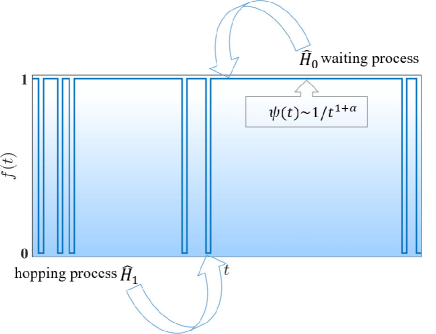
Figure 1: (Color online). Example of a typical trajectory of the stochastic driven quantum system. Control parameter $f(t)$ in the Hamiltonian. (1) equals to $1$ or $0$ corresponds to the duration of $\hat{H}_{0}$ and $\hat{H}_{1}$, respectively. The time for waiting process follows the power law distribution.

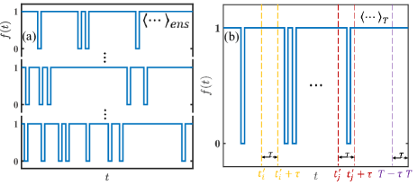
Figure 2: (Color online). Illustration to ensemble-averaged and time-averaged method in this paper. (a) $\langle\cdots\rangle_{ens}$ represents the quantity over different waiting time PDF trajectories. (b) $\langle\cdots\rangle_{T}$ represents the quantity over different time parts within a single waiting time PDF trajectory.

II Model and method

We consider a 1D single-particle model with Hamiltonian defined as:

$$\hat{H}(t)=f(t)\hat{H}_{0}+[1-f(t)]\hat{H}_{1},$$ (1)

where

$$\hat{H}_{0} =\sum_{i}{(-1)^{i}V\hat{c}_{i}^{\dagger}\hat{c}_{i}},$$ (2)

$$\hat{H}_{1} =\sum_{i}{-J\hat{c}_{i}^{\dagger}\hat{c}_{i+1}+h.c.}.$$ (3)

Where $\hat{H}_{1}$ and $\hat{H}_{0}$, including the free fermion hopping term and on-site potential term, correspond to the process of hopping and waiting governed by $f(t)$, respectively. $\hat{c}_{i}$ ($\hat{c}_{i}^{\dagger}$) denotes the annihilation (creation) operator of a spinless fermion on site $i$. The parameter $J$ represents the amplitude for nearest-neighbor (NN) single-particle hopping and $V$ is the on-site chemical potential. Open boundary condition is adapted.

Starting from an initial state $\phi(t=0)=\delta(i=L/2)$ where a particle is located at site $i=L/2$, the wave function $\phi(t)$ evolves according to the Schr$\ddot{\rm{o}}$dinger eqation $i\hbar\partial\hat{H}_{0}(t)/\partial t=\hat{H}_{0}(t)\phi(t)$, with the time $t$ for the waiting process following a power-law distribution $\psi(t)\propto 1/t^{1+\alpha}$, with $\alpha=0.65$ in the main text [it is applicable for other $\alpha$ values in Appendix A]. Then the particle starts hopping governed by the Hamiltonian $\hat{H}_{1}$ with $i\hbar\partial\hat{H}_{1}(t)/\partial t=\hat{H}_{1}(t)\phi(t)$, and the process is renewed. For simplification, the hopping time in the quantum model is quantified as lasting one second.

To quantify the transport behavior emerged in the driven quantum model, we introduce the squared width of the wavepacket $W^{2}(t)$, defined as:

$$W^{2}(t)=\sum_{i}\rho_{i}(t)[i-\bar{x}(t)]^{2},$$ (4)

where the density distribution $\rho_{i}(t)=\langle\phi(t)|\hat{c}_{i}^{\dagger}\hat{c}_{i}|\phi(t)\rangle$ and the center of matter (COM) of the wave packet $\bar{x}(t)=\sum_{i}i\rho_{i}(t)$. We can calculate the ensemble-averaged squared width of the wavepacket $\langle W^{2}(t)\rangle_{ens}$ over different waiting time PDF trajectories, as illustrated in Fig. 2(a).

In order to calculate the time-averaged squared width of the wavepackets $\langle W^{2}(t)\rangle_{T}$ for a given waiting time PDF trajectory, we consider the time evolution of the wave function over time $\tau$ at different initial position $t_{i}^{\prime}$, i.e., $|\phi(t_{i}^{\prime}+\tau)\rangle=\mathcal{\hat{T}}exp[-i\int_{t_{i}^{\prime}}^{\tau+t_{i}^{\prime}}\hat{H}(t^{\prime\prime})dt^{\prime\prime}]|\phi(t_{i}^{\prime})\rangle$. Where $\mathcal{\hat{T}}$ is the time-ordering operator. $\hat{H}(t^{\prime\prime})=\hat{H}_{0}$ or $\hat{H}_{1}$ is determined by whether the time $t^{\prime\prime}$ lies in the waiting or hopping process. For every finite total evolution time $T$, $t_{i}^{\prime}\in[0,T-t]$ with $i=1,2,..,\frac{T-t}{dt_{i}^{\prime}}$, as illustrated in Fig. 2(b). It is noteworthy that the width of the wavepacket has spread over many lattice sites after the evolution time interval $\tau$, making it necessary to reposition the particle at $\delta(i=L/2)$ at each time $t_{i}^{\prime}$, i.e., $|\phi(t_{i}^{\prime})\rangle=\delta(i=L/2)$. we can calculate a series of the squared width of the wavepackets defined in eq. (4) for different $t_{i}^{\prime}$. The time-averaged squared width of the wavepackets $\langle W^{2}(t)\rangle_{T}$ is then obtained by averaging these results. Additionally, for every finite total evolution time $T$, this quantity is also a random variable. Thus we consider its ensemble average $\langle\langle W^{2}(t)\rangle_{T}\rangle_{ens}$ over different waiting time PDF trajectories.

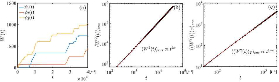
Figure 3: (Color online). (a) Width of the wavepacket under three different waiting-time PDFs. (b) Ensemble-averaged square width of the wavepackets. (c) Ensemble time-averaged square of width of the wavepackets. $L=8000$ for (a)-(b). $L=1200$ for (c). The solid (dashed) black (red) line with circular markers represents the real (fitted) data. The parameter $\Delta t=0.1J^{-1}$, $V=0$ and $\psi(t)\propto 1/t^{(1+\alpha)}$ with $\alpha=0.65$.

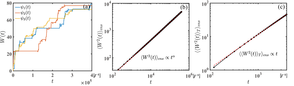
Figure 4: (Color online). (a) Width of the wavepacket under three different waiting-time PDFs. (b) Ensemble-averaged square width of the wavepackets. (c) Ensemble time-averaged square of width of the wavepackets. $L=2500$ for (a)-(b). $L=600$ for (c). The solid (dashed) black (red) line with circular markers represents the real (fitted) data. The parameter $\Delta t=0.1J^{-1}$, $V=4J$ and $\psi(t)\propto 1/t^{(1+\alpha)}$ with $\alpha=0.65$.

III Results

III.1 The case for free fermion

In this section, we first consider the wave function remaining unchanged during the waiting process, i.e., $V$ is always set to zero (zero-potential). Specifically, we start from an initial state $\phi(t=0)=\delta(i=L/2)$, the wave function $\phi(t)$ keeps unchanged [$\hat{H}_{0}=0$] for waiting time $t$ following a power-law distribution. Then the particle starts hopping governed by the Hamiltonian $\hat{H}_{1}$, and the process is renewed.

Fig. 3(a) intuitively exhibits three trajectories of the squared width of the wavepackets. We choose the discrete time step $\Delta t=0.1J^{-1}$ and system size $L=8000$, both shown to be sufficiently accurate in Appendix B. Considering $W(t)$ as a random variable dependent on different waiting-time PDFs $\psi_{i}(t)$, we calculate the ensemble-averaged squared width of the wavepackets $\langle W(t)^{2}\rangle_{ens}$ over $5\times 10^{4}$ waiting time PDF trajectories, as shown as a log-log plot in Fig. 3(b). We observe that it grows with time $t$ as a function of $t^{1.3155}$ ($\sim t^{2\alpha}$). Given that the jumping process corresponds to a free fermion hopping model within $W(t)\sim t$, ballistic transport behavior, we only restrict the particle waiting for time $t_{i}$ based on the ballistic transport behavior. This allows us to explain the result from classical point of view. Specifically, the PDF of displacement $x$ satisfies $\lambda(x)=\delta(x-1)$ for ballistic transport and $\psi(t)\propto 1/t^{(1+\alpha)}$ with $0<\alpha<1$. Their Fourier and Laplace transforms read as

$$\lambda(k) \sim 1+ik-\frac{1}{2}k^{2},$$ (5)

$$\psi(u) \sim 1-u^{\alpha}.$$ (6)

In fact, any pair of PDFs leading to finite $\langle x^{2}\rangle$ and $\langle t\rangle$ results in the same outcomes [Klafter et al., 1987]. Considering the variable $x$ and $t$ are independent of each other, so the PDF to find a walker at position $x$ and time $t$ is determined by

$$p(k,u)=\psi(u)\lambda(k)=1+ik-\frac{1}{2}k^{2}-u^{\alpha}.$$ (7)

The Fourier-Laplace transform [Metzler and Klafter, 2000; Klafter et al., 1987] is given by

$$P(k,u) =\frac{1-\psi(u)}{u}\frac{W_{0}(k)}{1-p(k,u)}$$

$$=\frac{2u^{\alpha-1}W_{0}(k)}{k(-2i+k)+2u^{\alpha}}.$$ (8)

Where $W_{0}(k)$ denotes the Fourier transform of the initial condition $W_{0}(x)=\delta(x-1)$. The time dependence of the moments of the displacement, $M_{n}(t)=\mathscr{L}^{-1}[(-i)^{n}\frac{\mathrm{d}^{n}P(k,u)}{\mathrm{d}k^{n}}]$ where $\mathscr{L}^{-1}$ is the inverse Laplace transform. Thus, we can derive the expressions for the first and second moments,

$$\langle x(t)\rangle =M_{1}(t)=\frac{W_{0}(k)}{\Gamma(1+\alpha)}t^{\alpha},$$

$$\langle x^{2}(t)\rangle =M_{2}(t)=\frac{W_{0}(k)}{\Gamma(1+\alpha)}t^{\alpha}+\frac{2W_{0}(k)}{\Gamma(1+2\alpha)}t^{2\alpha}.$$ (9)

Then the mean squared displacement of $x$ reads

$$\sigma^{2}[x(t)] =\langle x^{2}(t)\rangle-\langle x(t)\rangle^{2},$$

$$=\frac{W_{0}(k)}{\Gamma(1+\alpha)}t^{\alpha}+\left[\frac{2W_{0}(k)}{\Gamma(1+2\alpha)}-\frac{W_{0}^{2}(k)}{\Gamma^{2}(1+\alpha)}\right]t^{2\alpha}.$$ (10)

In the large $t$ limit where $t^{2\alpha}\gg t^{\alpha}$, eq. (III.1) reduced to $\sigma^{2}[x(t)]\sim t^{2\alpha}$. Therefore, the squared width of the wavepacket $W^{2}(t)$ correspond to the $\sigma^{2}[x(t)]$, $\sim t^{2\alpha}$.

On a parallel front, we calculate the time-averaged squared width of the wavepacket $\langle W^{2}(t)\rangle_{T}$ and its ensemble average $\langle\langle W^{2}(t)\rangle_{T}\rangle_{ens}$ over $5\times 10^{4}$ waiting time PDF trajectories, as shown in Fig. 3(c). Here, we choose the system size $L=1200$. We observe the quantity $\langle\langle W^{2}(t)\rangle_{T}\rangle_{ens}$ grows with time as a function of $t^{1.6387}$ $(\sim t^{1+\alpha})$, is not consistent with $\langle W^{2}(t)\rangle_{ens}$, indicating nonergodicity. This directly corresponds to the classical case where $\langle\delta(x)\rangle\neq 0$ and $\langle\langle W^{2}(t)\rangle_{T}\rangle_{ens}\sim t^{\alpha}t=t^{1+\alpha}$ as discussed in Ref  [He et al., 2008].

III.2 The effect of potential

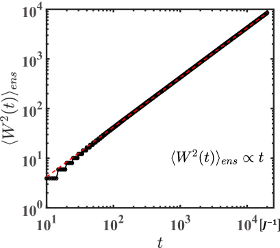
Figure 5: (Color online). Ensemble-averaged square of width of the wavepackets over $10^{4}$ samples. The solid (dashed) black (red) line with circular markers represents the real (fitted) data. The parameter $L=2500$, $\Delta t=0.01J^{-1}$ and $V(t)\propto 1/V^{(1+\alpha)}$ with $\alpha=0.65$.

In this section, we consider the effect of the on-site potential $V$. For simplicity, we set $V$ as a time-independent constant (constant-potential). Specifically, we start from an initial state $\phi(t=0)=\delta(i=L/2)$, the wave function $\phi(t)$ evolves according to $i\hbar\partial\hat{H}_{0}(t)/\partial t=\hat{H}_{0}(t)\phi(t)$ for waiting time $t$ following a power-law distribution. Then the particle starts hopping governed by the Hamiltonian $\hat{H}_{1}$ with $i\hbar\partial\hat{H}_{1}(t)/\partial t=\hat{H}_{1}(t)\phi(t)$, and the process is renewed.

Fig. 4(a) illustrates three particle trajectories with the potential amplitude $V$ set to $4J$. The ensemble-averaged squared width of the wavepackets $\langle W(t)^{2}\rangle_{ens}$ is shown as a log-log plot in Fig. 4(b). We observe that it grows with time $t$ as a function of $t^{0.6508}$ ($\sim t^{\alpha}$) which is different from the case mentioned in Sec. III.1. In this case, the unitary time evolution operator during the waiting process is given by $e^{-iH_{0}t}=e^{\pm iVt}$ [$H_{0}$ is diagonal], where the absolute value of global phase factor $Vt$ can become significantly large due to the PDF $\psi(t)$ satisfied a power law distribution. To determine which key element, $V$ or $t$, is more significant, we make $V$ follow the same power law distribution $\psi(V)\propto 1/V^{(1+\alpha)}$ and set the waiting time to four seconds to ensure the same global phase factor. The results are shown in Fig. 5. It reveals that the ensemble-averaged squared width of the wavepackets $\langle W(t)^{2}\rangle_{ens}\sim t$ and $\langle W(t)\rangle_{ens}\sim t^{0.5}$ [normal diffusion], indicating that the chemical potential $V$, with significant changes, is treated as white noise. Therefore, the presence of anomalous diffusive transport is a consequence of the long-tailed distribution of $t$ for the waiting process, which diminishes the amplitude and frequency of the wavepacket changes. Hence we can interpret the results shown in Fig. 4(b) from a classical perspective. The dynamics of the wavepacket adhere to normal diffusive behavior under the large amplitude of the phase factor, analogous to classical diffusion motion (Brownian motion) where $\lambda(x)=\frac{1}{2}\left[\delta(x-1)+\delta(x+1)\right]$. Thus, the eq. (5) is rewritten as $\lambda(k)\sim 1-k^{2}/2$, and the first and second moment are given by:

$$\langle x(t)\rangle =0,$$

$$\langle x^{2}(t)\rangle =M_{2}(t)=\frac{W_{0}(k)}{\Gamma(1+\alpha)}t^{\alpha}.$$ (11)

Then the mean squared displacement of $x$, $\sigma^{2}[x(t)]=\langle x^{2}(t)\rangle\sim t^{\alpha}$, which is consistent with our result.

Similarly, we calculate the time-averaged squared width of the wavepacket $\langle W^{2}(t)\rangle_{T}$ and its ensemble average $\langle\langle W^{2}(t)\rangle_{T}\rangle_{ens}$, as shown in in Fig. 4(c). Here, we choose the system size $L=600$. It reveals that the quantity grows with time as $t^{1.0102}$ $(\sim t)$, is not consistent with $\langle W^{2}(t)\rangle_{ens}$, indicating nonergodicity once again. It directly corresponds to the classical case where $\langle\delta(x)\rangle=0$ and $\langle\langle W^{2}(t)\rangle_{T}\rangle_{ens}\sim t$ as discussed in Ref  [He et al., 2008].

IV Conclusion and outlook

In conclusion, our work explores the quantum analog of the CTRW model, revealing various anomalous diffusive transport behaviors accompanied by the breakdown of ergodicity. For the zero-potential case, we observe that the ensemble-averaged squared width of the wavepackets grow with time as $t^{2\alpha}$, encompassing subdiffusive, superdiffusive and the standard diffusive motion. Additionally, the time-averaged square of width of wavepackets and its ensemble average grow with time as $t^{1+\alpha}$. The lack of convergence between these two averages indicates ergodicity breaking. For the constant-potential case, the ensemble-averaged squared width of the wavepackets grow with time as $t^{\alpha}$, corresponding to subdiffusive motion. Meanwhile, $\langle\langle W^{2}(t)\rangle_{T}\rangle_{ens}$ grows with time as $t^{1}$, signifying the recurrence of nonergodicity. The results highlight the abundant dynamics induced by the stochastic driving mechanism.

The power-law distribution is known for its ability to describe complex systems with a wide range of temporal scales. Up to this point, we have somewhat artificially set the long-tailed waiting time in our models. This raises an intriguing question: can we develop a model in which the time correlation of physical quantities naturally conforms to a power-law probability distribution? If successful, such a model would likely exhibit richer dynamics compared to those governed by exponential decay interactions.

V Acknowledgments

We thank Igor M. Sokolov for helpful and insightful suggestions on the continuous-time random walk. We also thank Zi Cai for the valuable discussions and guidance throughout this work. This work is supported by the National Key Research and Development Program of China (Grant No. 2020YFA0309000), NSFC of China (Grant No.12174251), the Natural Science Foundation of Shanghai (Grant No.22ZR142830), and the Shanghai Municipal Science and Technology Major Project (Grant No. 2019SHZDZX01).

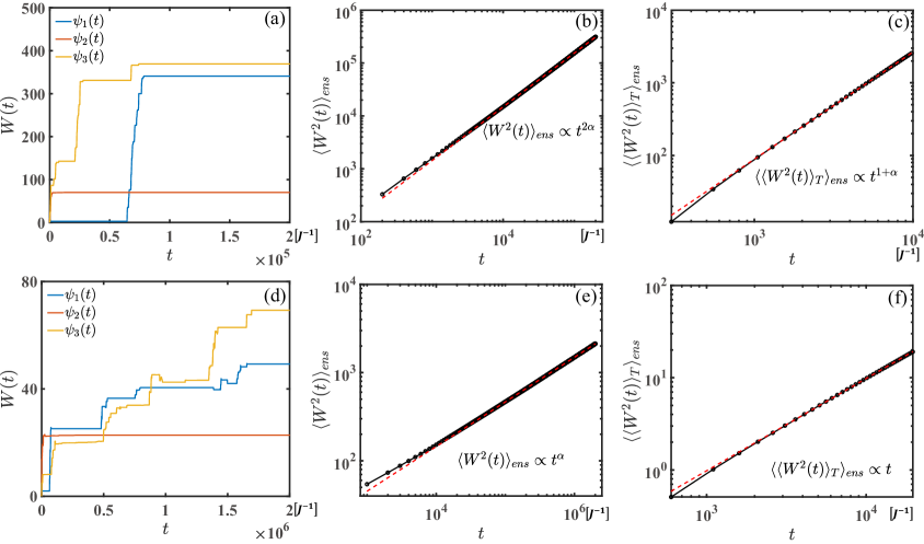
Figure 6: (Color online). (a)(d) Width of the wavepacket under three different waiting-time PDFs. (b)(e) [(c)(f)] Ensemble-averaged [time-averaged] square width of the wavepackets over $5\times 10^{4}$ samples. $L=6000$ for (a)(b) and $L=1600$ for (c). $L=2500$ for (d)(e) and $L=600$ for (f). The solid (dashed) black (red) line with circular markers represents the real (fitted) data for the right panel. The parameter $\Delta t=0.1J^{-1}$, $V=0$ ($V=4J$) for the upper (lower) panel and $\alpha=0.5$.

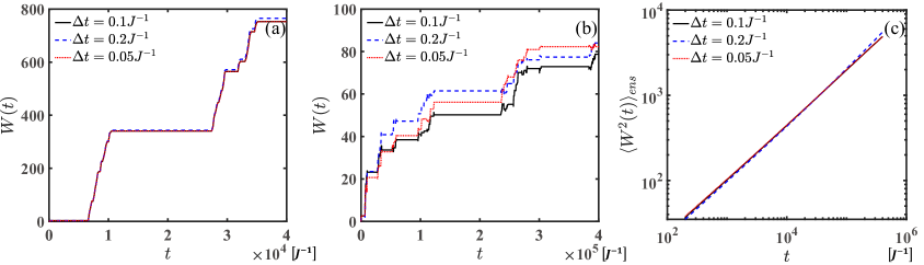
Figure 7: (Color online). Comparison between the width of the wavepacket for a waiting-time PDF with different $\Delta t$ with $V=0$ (a) and $V=4J$ (b)-(c). (c) Comparison between the ensemble-averaged square of width of the wavepackets over $5\times 10^{4}$ samples with different $\Delta t$. $L=8000$ for (a) and $L=2500$ for (b)-(c). $\alpha=0.65$.

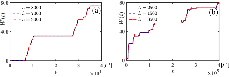
Figure 8: (Color online). Comparison between the width of the wavepacket for a waiting-time PDF with different system size $L$ with $V=0$ (a) and $V=4J$ (b). The parameter $\Delta t=0.1J^{-1}$ and $\alpha=0.65$.

Appendix A universal of numerical results

In the main text, we chose $\alpha=0.65$. The results are consistent for other $\alpha$ values between 0 and 1. As shown in the upper (lower) panel of Fig. 6, where $\alpha=0.5$, we observe the same behavior as with $\alpha=0.65$ for the zero-potential (constant-potential) case, indicating the universality of the anomalous transport behavior.

Appendix B Convergence of numerical results

B.1 Discrete time step dependence

Throughout the main text, we selected a discrete time step of $\Delta t=0.1J^{-1}$. The choice of $\Delta t$ is subtle because part of the system’s evolution time is composed of waiting time, which directly depends on $\Delta t$. To verify the convergence of our results with respect to $\Delta t$, we selected different $\Delta t$ values of $0.2J^{-1}$, $0.1J^{-1}$, and $0.05J^{-1}$, and compared their results. For the zero-potential shown in Fig. 7(a), our simulation results are consistent with the smaller $\Delta t=0.05J^{-1}$, indicating that the $\Delta t$ chosen is small enough to neglect numerical errors caused by the time discretization. For the constant-potential shown in Fig. 7(b), the results differs for different $\Delta t$, we infer that this is because the system continuously evolves due to the existence of $V$, so the state is slightly distinct for different $\Delta t$ when the hopping process starts, and the distinction can be amplified during time evolution. However, the non-convergence can be revised by the large number of samples because the small difference between these $\Delta t$ values almost does not affect the distribution of time $\psi(t)$. As shown in Fig. 7(c), the ensemble averaged square of width of wavepacket $\langle W^{2}(t)\rangle_{ens}$ is converged to the smaller $\Delta t=0.05J^{-1}$, indicating that the $\Delta t$ chosen in our simulation is sufficient.

B.2 System size dependence

The main text outlines a single-particle simulation on a 1D lattice with finite system sizes of $L=8000$ for the zero-potential case and $L=2500$ for the constant-potential case, which limits the maximum simulation time. After this period, the wave packet will reflect off the boundaries of the $1D$ lattice under open boundary conditions. It is necessary to check the system boundary dependence of our results. As shown in Fig. 8(a) and (b), the results converge well for different system sizes, indicating we have ruled out boundary effects.

References

- Montroll and Weiss (1965) E. W. Montroll and G. H. Weiss, Journal of Mathematical Physics 6, 167 (1965).
- Weiss (1994) G. H. Weiss, Journal of Statistical Physics 79, 497 (1994).
- Klafter and Sokolov (2011) J. Klafter and I. M. Sokolov, Oxford University Press (2011).
- Scher and Montroll (1975) H. Scher and E. W. Montroll, Phys. Rev. B 12, 2455 (1975).
- Bouchaud and Georges (1990) J.-P. Bouchaud and A. Georges, Physics Reports 195, 127 (1990).
- Barkai et al. (2000) E. Barkai, R. Metzler, and J. Klafter, Phys. Rev. E 61, 132 (2000).
- Weiss (2013) M. Weiss, Phys. Rev. E 88, 010101 (2013).
- Shlesinger (1974) M. F. Shlesinger, Journal of Statistical Physics 10, 421 (1974).
- Pfister and Scher (1977) G. Pfister and H. Scher, Phys. Rev. B 15, 2062 (1977).
- Geisel et al. (1985) T. Geisel, J. Nierwetberg, and A. Zacherl, Phys. Rev. Lett. 54, 616 (1985).
- Solomon et al. (1993) T. H. Solomon, E. R. Weeks, and H. L. Swinney, Phys. Rev. Lett. 71, 3975 (1993).
- Ohtsuki and Kawarabayashi (1997) T. Ohtsuki and T. Kawarabayashi, Journal of the Physical Society of Japan 66, 314 (1997).
- Mandelbrot (1963) B. Mandelbrot, The Journal of Business 36, 394 (1963).
- Masoliver et al. (2003) J. Masoliver, M. Montero, and G. H. Weiss, Phys. Rev. E 67, 021112 (2003).
- Scalas (2006) E. Scalas, Physica A 362, 225 (2006).
- Helmstetter and Sornette (2002) A. Helmstetter and D. Sornette, Phys. Rev. E 66, 061104 (2002).
- Mega et al. (2003) M. S. Mega, P. Allegrini, P. Grigolini, V. Latora, L. Palatella, A. Rapisarda, and S. Vinciguerra, Phys. Rev. Lett. 90, 188501 (2003).
- Hfling and Franosch (2013) F. Hfling and T. Franosch, Reports on Progress in Physics 76, 046602 (2013).
- Metzler and Klafter (2000) R. Metzler and J. Klafter, Physics Reports 339, 1 (2000).
- Sokolov et al. (2002) I. Sokolov, J. Klafter, and A. Blumen, Physics Today - PHYS TODAY 55, 48 (2002).
- Bouchaud (1992) J. P. Bouchaud, J. Phys. I France 2, 1705 (1992).
- Barkai and Margolin (2004) E. Barkai and G. Margolin, Israel Journal of Chemistry 44, 353 (2004).
- Margolin and Barkai (2005) G. Margolin and E. Barkai, Phys. Rev. Lett. 94, 080601 (2005).
- Lubelski et al. (2008) A. Lubelski, I. M. Sokolov, and J. Klafter, Phys. Rev. Lett. 100, 250602 (2008).
- He et al. (2008) Y. He, S. Burov, R. Metzler, and E. Barkai, Phys. Rev. Lett. 101, 058101 (2008).
- Zotos et al. (1997) X. Zotos, F. Naef, and P. Prelovsek, Phys. Rev. B 55, 11029 (1997).
- Batchelor (2005) M. T. Batchelor, Journal of Physics A: Mathematical and General 38, 3245 (2005).
- Miller et al. (2020) S. Miller, J. Tennyson, T. R. Geballe, and T. Stallard, Rev. Mod. Phys. 92, 035003 (2020).
- Karrasch et al. (2014) C. Karrasch, J. E. Moore, and F. Heidrich-Meisner, Phys. Rev. B 89, 075139 (2014).
- et al. (2016) M. , A. Scardicchio, and V. K. Varma, Phys. Rev. Lett. 117, 040601 (2016).
- Blake et al. (2017) M. Blake, R. A. Davison, and S. Sachdev, Phys. Rev. D 96, 106008 (2017).
- Friedman et al. (2020) A. J. Friedman, S. Gopalakrishnan, and R. Vasseur, Phys. Rev. B 101, 180302 (2020).
- Anderson (1958) P. W. Anderson, Phys. Rev. 109, 1492 (1958).
- Agarwal et al. (2015) K. Agarwal, S. Gopalakrishnan, M. Knap, M. Mller, and E. Demler, Phys. Rev. Lett. 114, 160401 (2015).
- Bar Lev et al. (2015) Y. Bar Lev, G. Cohen, and D. R. Reichman, Phys. Rev. Lett. 114, 100601 (2015).
- Luitz et al. (2016) D. J. Luitz, N. Laflorencie, and F. Alet, Phys. Rev. B 93, 060201 (2016).
- Bloch et al. (2008) I. Bloch, J. Dalibard, and W. Zwerger, Rev. Mod. Phys. 80, 885 (2008).
- Chang et al. (2018) D. E. Chang, J. S. Douglas, A. Gonzlez-Tudela, C.-L. Hung, and H. J. Kimble, Rev. Mod. Phys. 90, 031002 (2018).
- Polkovnikov et al. (2011) A. Polkovnikov, K. Sengupta, A. Silva, and M. Vengalattore, Rev. Mod. Phys. 83, 863 (2011).
- Luca D’Alessio and Rigol (2016) A. P. Luca D’Alessio, Yariv Kafri and M. Rigol, Advances in Physics 65, 239 (2016).
- Struck et al. (2012) J. Struck, C. lschlger, M. Weinberg, P. Hauke, J. Simonet, A. Eckardt, M. Lewenstein, K. Sengstock, and P. Windpassinger, Phys. Rev. Lett. 108, 225304 (2012).
- Cai et al. (2017) Z. Cai, C. Hubig, and U. Schollwöck, Phys. Rev. B 96, 054303 (2017).
- Harper et al. (2020) F. Harper, R. Roy, M. S. Rudner, and S. L. Sondhi, Annual Review of Condensed Matter Physics 11, 345 (2020).
- Guo et al. (2023) C. Guo, W. Cui, and Z. Cai, Phys. Rev. A 107, 033330 (2023).
- Sieberer et al. (2013) L. M. Sieberer, S. D. Huber, E. Altman, and S. Diehl, Phys. Rev. Lett. 110, 195301 (2013).
- Cai and Barthel (2013) Z. Cai and T. Barthel, Phys. Rev. Lett. 111, 150403 (2013).
- Marino and Diehl (2016) J. Marino and S. Diehl, Phys. Rev. Lett. 116, 070407 (2016).
- Lee et al. (2022) K. H. Lee, V. Balachandran, C. Guo, and D. Poletti, Phys. Rev. E 105, 024120 (2022).
- Erbanni et al. (2023) R. Erbanni, X. Xu, T. F. Demarie, and D. Poletti, Phys. Rev. A 108, 032619 (2023).
- (50) Y.-P. Wang, C. Fang, and J. Ren, arXiv:2310.03069 .
- (2024) M. , Phys. Rev. B 109, 075105 (2024).
- Zaburdaev et al. (2015) V. Zaburdaev, S. Denisov, and J. Klafter, Rev. Mod. Phys. 87, 483 (2015).
- Schuckert et al. (2020) A. Schuckert, I. Lovas, and M. Knap, Phys. Rev. B 101, 020416 (2020).
- Joshi et al. (2022) M. K. Joshi, F. Kranzl, A. Schuckert, I. Lovas, C. Maier, R. Blatt, M. Knap, and C. F. Roos, Science 376, 720 (2022).
- Nandy et al. (2017) S. Nandy, A. Sen, and D. Sen, Phys. Rev. X 7, 031034 (2017).
- Halimeh et al. (2018) J. C. Halimeh, M. Punk, and F. Piazza, Phys. Rev. B 98, 045111 (2018).
- Pan et al. (2020) L. Pan, X. Chen, Y. Chen, and H. Zhai, Nature Physics 16, 767 (2020).
- Kos et al. (2021) P. Kos, B. Bertini, and T. c. v. Prosen, Phys. Rev. Lett. 126, 190601 (2021).
- Cai (2022) Z. Cai, Phys. Rev. Lett. 128, 050601 (2022).
- Klafter et al. (1987) J. Klafter, A. Blumen, and M. F. Shlesinger, Phys. Rev. A 35, 3081 (1987).