What can we learn about Reionization astrophysical parameters using Gaussian Process Regression?

Abstract

Reionization is one of the least understood processes in the evolution history of the Universe, mostly because of the numerous astrophysical processes occurring simultaneously about which we do not have a very clear idea so far. In this article, we use the Gaussian Process Regression (GPR) method to learn the reionization history and infer the astrophysical parameters. We reconstruct the UV luminosity density function using the HFF and early JWST data. From the reconstructed history of reionization, the global differential brightness temperature fluctuation during this epoch has been computed. We perform MCMC analysis of the global 21-cm signal using the instrumental specifications of SARAS, in combination with Lyman-$\alpha$ ionization fraction data, Planck optical depth measurements and UV luminosity data. Our analysis reveals that GPR can help infer the astrophysical parameters in a model-agnostic way than conventional methods. Additionally, we analyze the 21-cm power spectrum using the reconstructed history of reionization and demonstrate how the future 21-cm mission SKA, in combination with Planck and Lyman-$\alpha$ forest data, improves the bounds on the reionization astrophysical parameters by doing a joint MCMC analysis for the astrophysical parameters plus 6 cosmological parameters for $\Lambda$CDM model. The results make the GPR-based reconstruction technique a robust learning process and the inferences on the astrophysical parameters obtained therefrom are quite reliable that can be used for future analysis.

1 Introduction

The epoch of reionization (EoR) represents a crucial period in the evolution history of the Universe, marking the transition from a neutral intergalactic medium (IGM) to the one that is fully ionized. This phase, occurring approximately between redshifts $z\approx 6$ and $z\approx 15$, hugely altered the thermal and ionization state of the Universe and set the stage for the formation and evolution of large-scale cosmic structures (Barkana & Loeb, 2001; Choudhury & Ferrara, 2005; Furlanetto et al., 2006; Pritchard & Loeb, 2012; Kuhlen & Faucher-Giguere, 2012). Reionization is primarily driven by the emergence of the first luminous sources, including Population II stars, galaxies, and quasars, which emitted copious amounts of ultraviolet (UV) photons capable of ionizing intergalactic hydrogen. The efficiency of these sources in producing ionizing photons, the fraction of photons that escape into the IGM, and the clumping of the IGM (Madau et al., 1999; Choudhury, 2009; Robertson et al., 2013; Bouwens et al., 2017) all play significant roles in shaping the reionization history. These factors collectively influence the reionization power spectrum as well as the global 21-cm signal, both of which serve as key observational probes of this epoch (Pritchard & Loeb, 2012; Furlanetto et al., 2006). However, having a clear understanding of the processes that drove reionization and their implications for cosmic evolution remains one of the foremost challenges in contemporary astrophysics.

Along with the lack of sufficient observational data from that epoch, one of the major hurdles towards this direction is a set of astrophysical parameters that govern the epoch of reionization and hence directly impact our understanding of the reionization history and the interpretation of observational data. It is quite a challenging task to constrain these parameters due to their complex interplay and limited observational data, which directly reflects on the (lack of) understanding of the physics of reionization. For instance, the clumping factor $C_{\rm HII}$, which accounts for the IGM’s inhomogeneity, is poorly constrained by observations, with recent simulations suggesting a wide range from 1 to 6 (Iliev et al., 2006; Pawlik et al., 2009; Finlator et al., 2012; Schroeder et al., 2013). Secondly, the number of photons entering the IGM depends on the production rate of Lyman continuum (LyC) photons by stars in galaxies, measured by the ionization efficiency $\xi_{\rm ion}$, a parameter that counts ionizing photons per unit UV luminosity. Another astrophysical parameter is the escape fraction $f_{\text{esc}}$, which is a measure of the fraction of photons entering the IGM thereby ionizing it, is poorly constrained due to the difficulty in observing the LyC photons beyond $z\sim 2-4.5$ (Inoue et al., 2014; Robertson, 2021). Earlier studies suggested a low $\xi_{\rm ion}$ and $f_{\text{esc}}\approx 0.2$, fitting more or less well with Cosmic Microwave Background (CMB) data from Planck and Hubble Frontier Fields (HFF) data (Robertson et al., 2013). In contrast, the latest James Webb Space Telescope (JWST) findings indicate a higher $\xi_{\rm ion}$, especially at $z>9$, highlighting the degeneracy between $\xi_{\text{ion}}$ and $f_{\text{esc}}$ (Muñoz et al., 2024; Simmonds et al., 2024; Atek et al., 2024). Recent studies by Kulkarni et al. (2019); Finkelstein et al. (2019); Cain et al. (2021); Katz et al. (2023) have also investigated any possible redshift evolution of $f_{\text{esc}}$. However, Mitra & Chatterjee (2023) suggest that a constant value of $f_{\text{esc}}$ between 0.06 and 0.1 for $z\geq 6$ is allowed by existing observational data. Thus, within the $\Lambda$CDM framework, magnitude-averaged product of $\xi_{\rm ion}$ and $f_{\rm esc}$ can vary widely depending on the model of reionization, raising significant questions about the validity of cosmological models inferred from reionization data (Hazra et al., 2020; Paoletti et al., 2021; Chatterjee et al., 2021; Dey et al., 2023a, b; Paoletti et al., 2024), which in turn reflects on the inference drawn about the reionization history as a whole.

In light of these widespread uncertainties related to the proper estimation of astrophysical parameters from direct approaches, searches for possible alternative tools that may help in having a somewhat better idea about them from the existing data alone, are natural questions the community has started to ask of late. One such interesting tool is the use of Machine learning (ML) techniques, that can significantly enhance our understanding of the epoch of reionization by developing flexible, data-driven models to analyze observational data. Unlike traditional methods, which depend on the assumption of predefined models that may overlook key details, ML techniques can uncover hidden patterns and relationships in complex data sets. These advanced inference methods can provide a better understanding of the astrophysical parameters, accounting for their variations across different redshifts (Krishak & Hazra, 2021; Mitra & Chatterjee, 2023), leading to unbiased, model-independent reconstructions of the reionization history and a relatively deeper insight into the underlying physics.

In the present article, we intend to enhance the understanding of reionization by examining the effects of various astrophysical parameters on its timeline. We employ an ML algorithm, Gaussian Process Regression (GPR) (Rasmussen & Williams, 2006) to perform a Bayesian, non-parametric, model-independent reconstruction of UV luminosity density $\log_{10}\rho_{\text{\rm UV}}$ as a function of redshift, using the current observations from Hubble Frontier Fields (HFF) (Lotz et al., 2017; Schenker et al., 2013; Ellis et al., 2013; McLure et al., 2013; McLeod et al., 2016; Oesch et al., 2018) compiled by (Bouwens et al., 2015b, 2017, 2021), early James Webb Space Telescope (JWST) (Harikane et al., 2023), and Subaru HSC’s Great Optically Luminous Dropout Research data (Harikane et al., 2022). This approach allows for flexible modeling of the evolution of ionizing sources without imposing restrictive parametric forms (Ishigaki et al., 2015, 2018; Adak et al., 2024). In this work, we seek to elucidate the factors driving reionization and contribute to mapping the Universe’s reionization history. As it will turn out, this will stem from a somewhat better hold on the astrophysical parameters through this GPR-based learning process.

We begin by reviewing the theoretical framework that describes the ionization state of the IGM, highlighting significant astrophysical parameters and their connection to observables. In addition to UV luminosity data sets, we consider the neutral hydrogen fraction measurements (Greig et al., 2017; Davies et al., 2018; Totani et al., 2006; McQuinn et al., 2008; Bolton et al., 2011; Mortlock et al., 2011; Ono et al., 2012; Schenker et al., 2014; Tilvi et al., 2014; Mason et al., 2019) and optical depth $\tau_{\text{reio}}$ constraints from the Planck 2018 release of Cosmic Microwave Background (CMB) observations (Planck Collaboration et al., 2020) to obtain the reionization history as a function of redshift. For this exercise, we perform a full Bayesian Markov Chain Monte Carlo (MCMC) analysis to explore the role of existing data sets in predicting the observationally favoured bounds on the reionization astrophysical parameters.

Further, one of the most exciting probes of the EoR is the spin-flip line of neutral hydrogen, with a rest frame wavelength of 21-cm. Advancements in current instruments and upcoming missions are expected to revolutionize 21-cm cosmology from observational point of view, providing highly significant measurements of both the power spectrum and the global 21-cm brightness temperature signal (Pritchard & Loeb, 2012). Currently, the Shaped Antenna measurement of the background RAdio Spectrum (SARAS) (Patra et al., 2013) aims to measure the global sky-averaged 21-cm signal from the cosmic dawn and the EoR using a shaped antenna to capture the redshifted 21-cm line (Singh et al., 2018). In the coming decade, experiments like the Square Kilometre Array (SKA) (de Lera Acedo et al., 2015), Hydrogen Epoch of Reionization Array (HERA) (Abdurashidova et al., 2022) and other significant missions (van Haarlem et al., 2013), will drive advancements in cosmology by detecting the 21-cm neutral hydrogen signal from the early Universe. By employing 21-cm intensity mapping techniques, SKA will track neutral hydrogen in the Universe, yielding comprehensive insights into the post-reionization and reionization epochs, as well as the cosmic dawn, up to a redshift of 30 (Pritchard & Loeb, 2012). Our study explores how the ongoing SARAS and next-generation SKA, with their innovative approaches, will enhance our understanding of reionization by reconstructing the reionization history and refining the bounds on the associated astrophysical parameters.

We thus detail our methodology for analyzing the global 21-cm signal and the reionization power spectrum within the framework of the $\Lambda$CDM cosmological model. For the global 21-cm signal $\Delta T_{b}$, we generate a mock $\Delta T_{b}$ vs $z$ data, assuming the instrumental specifications of SARAS (Patra et al., 2013), considering the best-fit values of these astrophysical parameters obtained using the existing data sets. For the power spectrum analysis, we use the instrumental specifications of SKA to generate a mock data set (Dewdney & Braun, 2016), using the Planck 2018 best-fit $\Lambda$CDM model. We make prior modifications in CLASS (Blas et al., 2011) to incorporate the contribution from the GP reconstructed reionization history profile (instead of the inbuilt $\tanh$ reionization model), to compare both the cases and reflect on their outcomes. In the final step, we conduct a comprehensive Bayesian MCMC analysis to investigate how SARAS and upcoming SKA will aid in probing the astrophysical parameters of reionization.

Our work advances from the earlier works in this direction (see, for example, Krishak & Hazra (2021); Chatterjee et al. (2021); Paoletti et al. (2021); Adak et al. (2024)) by multiple folds: First, we employ GPR by simultaneously training the parameters governing the GP mean function and the kernel hyperparameters (instead of fixing the mean function to the best-fit values) to obtain the predicted UV luminosity density profile. Secondly, along with other astrophysical parameters, we keep the clumping factor $C_{\rm HII}$ as a free parameter in MCMC analysis (and compare with earlier studies with a fixed value $C_{\rm HII}$ = 5). Third, we consider both HFF and JWST as the reconstruction training data sets (along with possible combinations of other data sets), followed by a thorough, methodical comparative analysis between their role in constraining the astrophysical parameters and hence in deriving reionization history. On top of that, we extend our analysis to the yet-unexplored directions on the applications of GPR in reionization. This is materialized by considering, separately, the global 21-cm signal (from SARAS) and 21-cm power spectrum (from SKA), that helps in exploring their role in inferring the reionization physics. And finally, we modify the Boltzmann solver code CLASS (Blas et al., 2011) to accommodate our reconstructed reionization history into the MCMC code MontePython (Audren et al., 2013; Brinckmann & Lesgourgues, 2019). Thus, our findings are expected to have important implications for understanding the nature and distribution of the first light sources and their role in shaping the early Universe.

2 Reionization and observables

2.1 Global Brightness Temperature Fluctuation

The key observable in 21-cm cosmology is the global brightness temperature fluctuation, which is the difference between the spin temperature (related to the neutral hydrogen number densities in different atomic levels) and the background temperature. The total brightness temperature at redshift $z$ is given by the temperature of the background radiation field, with some fraction of it absorbed and re-emitted due to 21-cm hyperfine transitions in neutral hydrogen atoms. The properties of HI in absorption and emission are described by the spin temperature $T_{s}$ and the optical depth $\tau$ (Pritchard & Loeb, 2012; Furlanetto et al., 2006):

$$T_{\rm b}=T_{s}(1-e^{-\tau})+T_{\gamma}e^{-\tau}\,.$$ (1)

Due to the low probability of a 21-cm transition, the optical depth is typically small. The differential brightness temperature can thus be written as linear in $\tau$:

$$\Delta T_{\rm b}=\frac{T_{s}-T_{\gamma}}{1+z}\left(1-e^{-\tau}\right)\approx\frac{T_{s}-T_{\gamma}}{1+z}\tau\,.$$ (2)

The optical depth produced by a patch of neutral hydrogen at the mean density and with a uniform 21-cm spin temperature $T_{s}$,

$$\tau=9.0\times 10^{-3}\left(\dfrac{T_{\text{CMB}}}{T_{s}}\right)\left(\dfrac{\Omega_{\rm b}h}{0.03}\right)\left(\dfrac{\Omega_{\rm m}}{0.3}\right)^{-1/2}\left(\dfrac{1+z}{10}\right)^{1/2}\,.$$ (3)

The Lyman-$\alpha$ (Ly$\alpha$) and X-ray radiation backgrounds during the epoch of reionization are anticipated to be strong enough to equalize the spin temperature $T_{s}$ with the gas temperature and heat up the cosmic gas well above the CMB temperature (Madau et al., 1997). In these circumstances, the observed 21-cm brightness temperature $T_{b}$, in relation to the CMB temperature $T_{\gamma}$, becomes independent of $T_{s}$. Consequently, $T_{b}$ (hereafter measured relative to $T_{\gamma}$) is given by (Morandi & Barkana, 2012)

$$\Delta T_{b}=(T_{s}-T_{\gamma})(1-e^{-\tau})~{}Q_{\rm HI}\approx T_{21}\left(\dfrac{1+z}{10}\right)^{1/2}Q_{\rm HI}\,,$$ (4)

where $T_{21}=9.0\times 10^{-3}(\Omega_{\rm b}h/0.03)(\Omega_{\rm m}/0.3)^{-1/2}\,T_{\text{CMB}}=27.2$ mK and $Q_{\rm HI}$ is the neutral hydrogen fraction. We focus solely on the cosmic mean neutral or ionized fraction and disregard spatial fluctuations in the 21-cm signal caused by density and peculiar velocity variations.

2.2 Power Spectrum

The difference between the 21-cm temperature $T_{b}(\mathbf{x})$ and the average temperature $\overline{T}_{b}(z)$ at a given redshift can be calculated at any spatial point and is denoted by $\Delta T_{b}(\bf x)$. Its Fourier transform is indicated as $\Delta T_{b}(\bf x)$. The two-point correlation function of 21-cm temperature fluctuations at redshift $z$ is written as

$${\Delta T_{b}(\mathbf{k})\Delta T_{b}(\mathbf{k}^{\prime})}\equiv P_{21}(\mathbf{k},z)(2\pi)^{3}\delta_{D}{(\bf k-k^{\prime})}\,,$$ (5)

with

$$P_{21}(\mathbf{k},z)=\left[{\cal A}(z)+\overline{T}_{b}(z)\mu^{2}\right]^{2}P_{\rm HI}(k,z)\,,$$ (6)

here, ${\cal A}(z)=\mathrm{d}T_{21}/\mathrm{d}\delta_{b}$ indicates a function of $z$, $\mu\equiv k_{||}/k$ is the cosine of the angle between the line-of-sight $k_{||}$ and the total wave vector $k$, and $P_{\rm HI}$ is the power spectrum for the perturbations in neutral hydrogen density, which matches $P_{\delta}$ in the scales of interest.

The spin temperature $T_{s}$ during the EoR is coupled to the gas temperature through the Wouthuysen-Field effect (Wouthuysen, 1952; Hirata, 2006). The star formation heats the gas, which give rise the spin temperature above the CMB temperature $T_{\gamma}$, making the 21-cm line appear in emission. In this epoch, we can express the factors in Eq.  (6) as

$$\mathcal{A}(z)=\overline{T}_{21}(z)=27.3\,{\rm mK}\,\times\overline{x}_{\rm H}\dfrac{T_{s}-T_{\gamma}}{T_{s}}\left(\dfrac{1+z}{10}\right)^{1/2}\,,$$ (7)

here we can drop the temperature factor since $T_{s}\gg T_{\gamma}$, and $\overline{x}_{\rm H}$ represents the mean neutral hydrogen fraction

Assuming an antenna array with a baseline $D_{\rm base}$ uniformly covered to a fraction $f_{\rm cover}\leq 1$ and an observation time of $t_{o}$, the instrumental-noise power spectrum in $k$-space is given by (Zaldarriaga et al., 2004; Tegmark & Zaldarriaga, 2009)

$$P^{N}_{21}(z)=\dfrac{\pi T_{\rm sys}^{2}}{t_{o}f_{\rm cover}^{2}}\chi^{2}(z)y_{\nu}(z)\dfrac{\lambda^{2}(z)}{D_{\rm base}^{2}}\,,$$ (8)

In this context, $\lambda(z)$ is the 21-cm transition wavelength corresponding to redshift $z$, $y_{\nu}(z)=18.5,\sqrt{(1+z)/10}$ Mpc/MHz serves as the conversion function from frequency $\nu$ to $k_{||}$, and the system temperature $T_{\rm sys}$ is predominantly determined by galactic synchrotron emission, characterized as (de Oliveira-Costa et al., 2008)

$$T_{\rm sys}=180\,{\rm K}\times\left(\dfrac{\nu}{180\,\rm MHz}\right)^{-2.6}\,.$$ (9)

Combining all these pieces of information, the observed power spectrum looks (Sprenger et al., 2019; Dey et al., 2023b)

$$P_{\rm 21,obs}(k,\mu,z)=f_{\rm AP}(z)\times f_{\rm res}(k,\mu,z)\times f_{\rm RSD}(\hat{k},\hat{\rm\mu},z)\times P_{\rm 21}(k,z)+P^{N}_{\rm 21}(z)\,,$$ (10)

where $P_{\rm 21}(\mathbf{k},z)$ denotes the 21-cm power spectrum. In the above formula, we have applied the flat-sky approximation, which provides a specific definition of the line-of-sight distance vector $\vec{r}$ and Fourier modes. This approximation breaks the isotropy along the observer’s line of sight but retains the symmetry perpendicular to it. The coordinate relations are as follows: $k=|\vec{k}|$, $\mu=\dfrac{\vec{k}\cdot\vec{r}}{kr}$, with the parallel component of the mode being $k_{\rm\parallel}=\mu k$ and the perpendicular component being $k_{\rm\perp}=k\sqrt{1-\mu^{2}}$.

3 Data sets

As stated earlier, in the process of learning the reionization history, we have two-fold goals: (i) to find out the present constraints from a couple of cosmological data sets that also help in the reconstruction process and (ii) to forecast on the astrophysical parameters along with the cosmological parameters from the 21-cm powers spectra.

For current constraints, the data sets used are the following:

• UV17(A): The derived UV luminosity function (LF) density data (Bouwens et al., 2015a, 2017) at $z$ $\sim$ 4-10 from HFF observations (Lotz et al., 2017) with truncation magnitude $M_{\rm trunc}=-17$.

• UV17(B): The UV LF data for $z\sim 2-7$, derived in using the HUDF, HFF, and CANDELS fields, compiled by (Bouwens et al., 2015a; Ishigaki et al., 2018). For $z\sim 4-7$, we incorporate data from the Hyper Suprime-Cam (HSC) Subaru Strategic Program (SSP) survey (Harikane et al., 2022). For $z\sim 8-10$, we consider the derived LF obtained by Bouwens et al. (2023); Adak et al. (2024) and early JWST data at $z\sim 9$ and 12 (Harikane et al., 2023).

• QHII: Neutral hydrogen fraction measurements from Ly$\alpha$ emission from galaxies (Ono et al., 2012; Schenker et al., 2014; Tilvi et al., 2014; Mason et al., 2019), damping wings of gamma-ray bursts (Totani et al., 2006; McQuinn et al., 2008), dark gap in quasar spectra (McGreer et al., 2015) and ionized zones near high redshift quasars (Mortlock et al., 2011; Bolton et al., 2011).

• Planck: The optical depth constraints $\tau_{\rm reio}=0.054\pm 0.007$ from Planck 2018 release of Cosmic Microwave Background observation (Planck Collaboration et al., 2020).

• SARAS: Mock data generated from the instrumental specifications of the global 21-cm mission (Patra et al., 2013).

On the other hand, for future forecasts from 21-cm power spectra, we make use of the following data sets:

• Planck: Fake Planck 2018 data (Planck Collaboration et al., 2020; Sprenger et al., 2019), which is used for forecast analysis in MontePython (Audren et al., 2013; Brinckmann & Lesgourgues, 2019).

• Ly$\alpha$: MIKE-HIRES Lyman-$\alpha$ forest data set (Viel et al., 2013).

• SKA: Mock data generated using the instrumental specifications of SKA-Low (Dewdney & Braun, 2016).

4 Methodology

The ionization equation describes the time evolution of the volume filling factor of ionized hydrogen in the intergalactic medium, $Q_{\rm HII}$, by a first-order ordinary differential equation,

$$\frac{\mathrm{d}Q_{\rm HII}}{\mathrm{d}t}=\frac{\dot{n}_{\text{ion}}}{\langle n_{\rm H}\rangle}-\frac{Q_{\rm HII}}{t_{\text{rec}}}\,.$$ (11)

The source term $\dot{n}_{\text{ion}}$ is characterized by the rate of production of ionizing photons, which depends on (i) the UV luminosity density function $\rho_{\rm UV}$, (ii) the efficiency of the source to produce ionizing photons $\xi_{\text{ion}}$, (iii) the fraction of photons that escape into the IGM $f_{\text{esc}}$. It is defined as $\dot{n}_{\text{ion}}=\rho_{\rm UV}\langle f_{\text{esc}}\xi_{\text{ion}}\rangle$, where $\langle f_{\text{esc}}\xi_{\text{ion}}\rangle$ is a magnitude-averaged product. The sink term in the ionization equation accounts for the recombination process in the IGM. The recombination time $t_{\text{rec}}$ is determined by the recombination coefficient $\alpha_{B}(T)$ and the clumping factor $C_{\rm HII}$; $t_{\text{rec}}=\left[{C_{\rm HII}\,\alpha_{B}(T)\left(1+\frac{Y_{p}}{4X_{p}}\right)\langle n_{\rm H}\rangle(1+z)^{3}}\right]^{-1}$ where $n_{\rm H},n_{\rm He},n_{\rm HII}$ are the number densities of hydrogen, helium, and ionized hydrogen respectively. $X_{p},Y_{p}$ are the primordial mass fractions of hydrogen and helium. The $C_{\rm HII}$ accounts for the inhomogeneity of the IGM, and is not very well constrained from observations. Our analysis assumes the IGM temperature $T$ is fixed at 20,000 K. In this work, we will first reconstruct the UV luminosity density using GPR. Subsequently, we will use the reconstructed values of $\log_{10}\rho_{\text{\rm UV}}$ to derive the reionization history.

4.1 Reconstructing the UV luminosity density

The evolution of the UV luminosity density with redshift can be obtained by parametric (Yu et al., 2012; Ishigaki et al., 2015, 2018; Adak et al., 2024) and non-parametric free-form methods (Hazra et al., 2020; Paoletti et al., 2021) to determine $n_{\text{ion}}$. Recently, a model-independent reconstruction of $\rho_{\rm UV}$ by (Krishak & Hazra, 2021) invalidates the single power-law form (Yu et al., 2012), as it fails to account for the decline at $z\sim 8$, resulting in an incorrect Thomson scattering optical depth. Therefore, the assumption of a parametric logarithmic double power law (Ishigaki et al., 2015, 2018), given by

$$\rho_{\rm UV}(z) = \frac{2\rho_{{\rm UV},z=z_{1}}}{10^{a(z-z_{1})}+10^{b(z-z_{1})}}~{}\,,$$ (12)

to describe the UV LF profile is a better ansatz, characterised by four distinct parameters, namely - the amplitude ($\rho_{{\rm UV},z=z_{1}}$), two tilts ($a,b$) and the redshift ($z_{1}$) at which the tilt in the power changes.

While parametric methods are useful, the functional form restricts their ability to address the data in several instances [see (Yu et al., 2012; Ishigaki et al., 2018; Adak et al., 2024)]. So, a more robust approach is a non-parametric reconstruction which attempts to reconstruct the cosmic reionization history directly from the observational data. In this article, we use Gaussian Process Regression (Rasmussen & Williams, 2006; Seikel et al., 2012; Shafieloo et al., 2012; Mukherjee, 2022; Shah et al., 2023; Mukherjee et al., 2024b), aka, GPR for a Bayesian, non-parametric reconstruction of luminosity density in a model-independent manner.

A Gaussian Process (GP) is a collection of random variables such that the joint distribution of any finite subset of it is described by a multivariate Gaussian. It is characterized by a mean function $\mu(\mathrm{x})$ and covariance function $k(\mathrm{x},\mathrm{x^{\prime}})$, where for a real process $f(\mathrm{x})$, we have $\mu(\mathrm{x})=\mathbb{E}[f(\mathrm{x})]$, and $k(\mathrm{x},\mathrm{x^{\prime}})=\mathbb{E}[(f(\mathrm{x})-\mu(\mathrm{x}))(f(\mathrm{x^{\prime}})-\mu(\mathrm{x^{\prime}}))]$. For a finite set of training points $\mathrm{x}=\{x_{i}\}$, a function $f(\mathrm{x})$ evaluated at each $x_{i}$ can be represented by a random variable with a Gaussian distribution, such that the vector $\mathrm{f}=\{f_{i}\}$ has a multivariate Gaussian distribution given as $\mathrm{f}\sim\mathcal{N}\left(\mu(\mathrm{x}),C(\mathrm{x},\mathrm{x})\right)$, where $C$ is the covariance matrix characterized by the kernel or covariance function $k(x_{i},x_{j})$, which gives the covariance between two random variables $x_{i}$ and $x_{j}$ respectively. For our analysis, we choose the kernel to be the Radial Basis Function represented as $k(x_{i},x_{j})=\sigma_{f}\,\text{exp}\left[-\frac{(x_{i}-x_{j})^{2}}{2l^{2}}\right]$, with the correlation length $l$ and amplitude $\sigma_{f}$. The logarithmic double power law parametrization, given in Eq. (12) is considered a mean function, whose parameters are jointly constrained with the kernel hyperparameters, marginalizing the log-marginal likelihood via a Bayesian Markov Chain Monte Carlo (MCMC) analysis with emcee (Foreman-Mackey et al., 2013). We undertake this exercise for both UV17(A) and UV17(B) compilations of the luminosity density data as the training set. Although our reconstruction method is somewhat in the same vein of Krishak & Hazra (2021), where the mean function is fixed to the best-fit values obtained by $\chi^{2}$ minimization, our novelty lies in simultaneously training the parameters governing the GP mean function and the kernel hyperparameters to obtain the predicted UV luminosity density profile, which helps the predictions arise from a symbiotic environment and hence is expected to generate more realistic outcome of the learning process.

4.2 Learning the reionization history

On having reconstructed the profile of UV luminosity density in a model-independent way, we now re-define the values of $\log_{10}\rho_{\rm UV}$ in four distinct equidistant nodes in the range $4<z<12$. Our approach is akin to Gerardi et al. (2019), where this range is selected to fully encompass available UV17(A) and UV17(B) data sets. The values of the UV luminosity density at these four nodes i.e., $\log_{10}\rho_{1-4}$ are taken as free parameters in MCMC sampling, employing emcee (Foreman-Mackey et al., 2013), to learn the reionization history by solving the ionization Eq. (11) using this model-independent form. At each MCMC step, these points serve as training data for GP regression. Hence, GP reconstruction yields samples of the history of UV luminosity densities, based on the training input configurations.

For this full Bayesian analysis, we take into account different combinations of the existing data sets, described in Sec. 3. In the ionization equation, we treat $\left\langle f_{\text{esc}}\xi_{\text{ion}}\right\rangle$ as a single parameter by incorporating $f_{\text{esc}}$ into $\xi_{\text{ion}}$ (Dayal & Ferrara, 2018). Following Price et al. (2016), we apply a uniform prior on $\log_{10}\xi_{\text{ion}}\in\mathcal{U}[23.5,27.5]$ in units of $\log_{10}\left[\text{Hz}\,\text{erg}^{-1}\right]$. The clumping factor is initially treated as a free parameter with a uniform prior, setting an upper bound at $C_{\rm HII}\leq 10$. Later on, it is kept fixed at $C_{\rm HII}=5$, similar to Krishak & Hazra (2021). This helps us explore the outcome of both the cases for a comparative analysis.

In the final stage, we modify the public version of the Boltzmann solver code CLASS (Blas et al., 2011), where this reconstructed reionization history is supplied as an input within the thermodynamics.c module, in place of the Planck $\tanh$ reionization model. This helps us consistently overcome any dependence of the baseline reionization model on the estimated parameters and search for possible consequences of the present learning method. For this we undertake a joint MCMC analysis on the 6 $\Lambda$CDM cosmological parameters and 2 reionization astrophysical parameters using MontePython (Audren et al., 2013; Brinckmann & Lesgourgues, 2019) by generating mock data for the upcoming 21-cm SKA mission along with some other data sets mentioned in Sec. 3. We subsequently analyze the errors and correlations of the different model parameters.

5 Results & Discussions

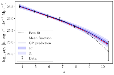
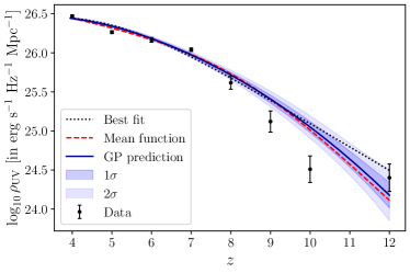
Figure 1: The reconstructed UV luminosity density function in the redshift range $z\sim 4-12$ obtained from Gaussian process regression using the UV17(A) (left panel) and UV17(B) (right panel) data.

Following the methodology described in Sec. 4.1, we reconstruct the UV luminosity density as a function of redshift in the range $4<z<12$ employing GPR on the UV17(A) and UV17(B) data sets. Fig. 1 illustrates the reconstructed UV luminosity density profile as a function of redshift for both UV17(A) and UV17(B) compilation, shown in the respective left and right panels. The solid blue curve represents the GP reconstructed mean curve, and the shaded regions correspond to the 1$\sigma$ and 2$\sigma$ uncertainties associated with the reconstructed curve. The black dotted lines give the best-fit curves assuming the logarithmic double power-law parametric form to model the $\log_{10}\rho_{\rm UV}$ data. The predicted logarithmic double power-law evolution as a mean function for GPR is shown with red dashed lines. Our findings indicate that the logarithmic double power law model is consistent with the reconstructed GP function and the UV17(A) and UV17(B) data within the redshift range $4<z<8$. For $z>9$, the mean reconstructed curve deviates from the best-fit values. However, this deviation is included within 2$\sigma$ for the right panel of Fig. 1, and excluded from 2$\sigma$ in the left panel of Fig. 1, respectively. In the case of UV17(B) data, the reconstructed UV luminosity curve excludes the $z=9$ and $z=10$ JWST $\log_{10}\rho_{\rm UV}$ data points.

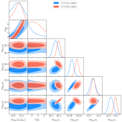
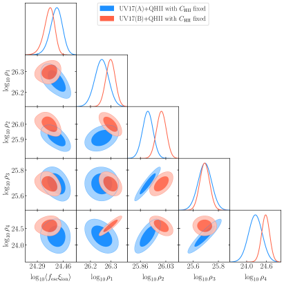
Figure 2: Comparison between the constraints obtained on the astrophysical parameters employing the UV17(A)+QHII vs UV17(B)+QHII (left panel) and UV17(A)+QHII vs UV17(B)+QHII with the clumping factor kept constant at $C_{\rm HII}$=5 during the MCMC (right panel).

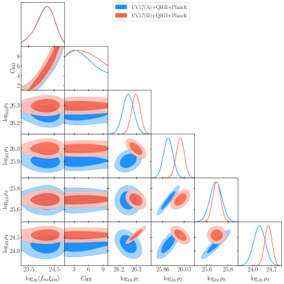
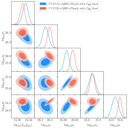
Figure 3: Comparison between the constraints obtained on the astrophysical parameters employing the UV17(A)+QHII+Planck vs UV17(B)+QHII+Planck (left panel) and UV17(A)+QHII+Planck vs UV17(B)+QHII+Planck with the clumping factor kept constant at $C_{\rm HII}$=5 during the MCMC (right panel).

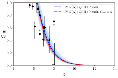
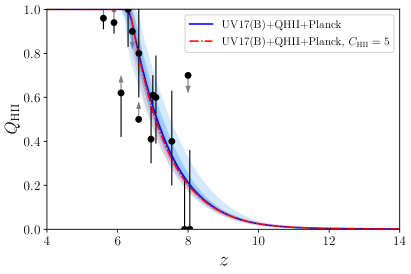
Figure 4: Evolution of the ionization fraction obtained using UV17+QHII+Planck (blue curve) vs UV17+QHII+Planck for a fixed value of the clumping factor (red dashed line) from the GP reconstruction of the UV luminosity density with the UV17(A) (left panel) and UV17(B) (right panel) compilation.

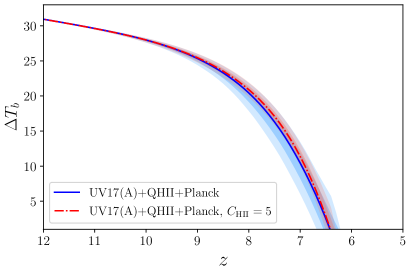
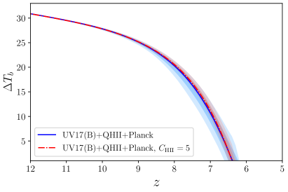
Figure 5: Reconstruction of the global 21-cm signal at reionization epoch obtained using UV17+QHII+Planck (blue curve) vs UV17+QHII+Planck for a fixed value of the clumping factor $C_{\rm HII}=5$ (red dashed line) from the GP reconstruction of the UV luminosity density with the UV17(A) (left panel) and UV17(B) (right panel) compilation.

With this reconstructed UV luminosity profile, we proceed to trace the evolution of the ionization fraction $Q_{\rm HII}$, following the methodology described in Sec. 4.2. For this we adopt four equidistant redshift nodes at $z_{1}=4$, $z_{2}=6$, $z_{3}=8$ and $z_{4}=10$, where the values of logarithmic UV luminosity densities are redefined as $\log_{10}\rho_{1}$, $\log_{10}\rho_{2}$, $\log_{10}\rho_{3}$ and $\log_{10}\rho_{4}$ respectively. We make use of Eq. (11) to solve for $Q_{\rm HII}$ where the reconstructed values of the UV luminosity densities (at the 4 redshift nodes) are treated as free parameters during in the Bayesian MCMC analysis. The entire exercise is undertaken employing different data sets, mentioned in Sec. 3, namely, UV17(A) & UV17(B) in combination with QHII Ly$\alpha$ and Planck $\tau_{\rm reio}$ data. Fig. 2 shows the 2D-confidence contours and 1D-marginalized posteriors for the relevant parameters upon MCMC done using the joint UV17(A)+QHII (in blue) and UV17(B)+QHII (in red) data sets. Similarly, Fig. 3 depicts the same for UV17(A)+QHII+Planck (in blue) and UV17(B)+QHII+Planck (in red) combinations. It should be noted that, in the left panel of Figs. 2 and 3, the clumping factor $C_{\rm HII}$ is treated as a free parameter during MCMC, whereas the right panel shows the case when the value of the clumping factor is kept fixed at $C_{\rm HII}=5$ respectively. For both figures, we find that the parameters $\log_{10}\left\langle f_{\rm esc}\xi_{\rm ion}\right\rangle$ and $C_{\rm HII}$ are positively correlated. This feature indicates an anti-correlation with $t_{\rm rec}$, i.e., a reduction in $\left\langle f_{\rm esc}\xi_{\rm ion}\right\rangle$ lowers the source term, which is only offset by a longer recombination period to maintain ionization [see Gorce et al. (2018); Mason et al. (2019); Paoletti et al. (2021); Krishak & Hazra (2021)]. The values of UV luminosity densities at redshift points $z_{1}$, $z_{2}$, and $z_{4}$ differ greatly between the two different combinations of the data sets. However, at $z_{3}$, the average values are very similar, where the inclusion of early JWST data in the UV17(B) compilation narrows down the range of possible values. We also find that the nature of correlations between the parameters $\log_{10}\rho_{1-4}$ remains unchanged on fixing the value of $C_{\rm HII}$ (for comparison see left and right panels of Figs. 2 and 3).

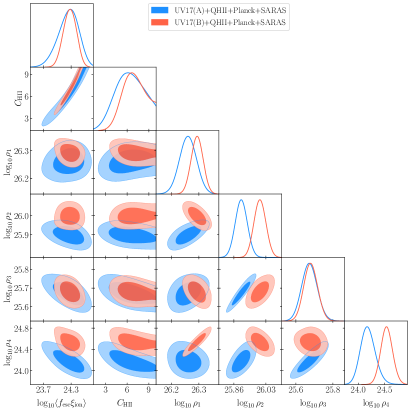
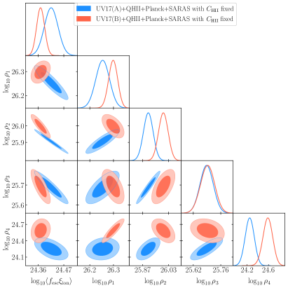
Figure 6: Comparison between the constraints obtained on the astrophysical parameters employing the UV17(A)+QHII+Planck+SARAS vs UV17(B)+QHII+Planck+SARAS (left panel) and UV17(A)+QHII+Planck+SARAS vs UV17(B)+QHII+Planck+SARAS with the clumping factor kept constant at $C_{\rm HII}$=5 during the MCMC (right panel).

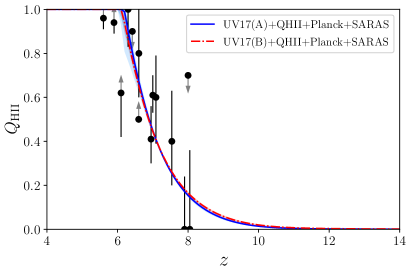
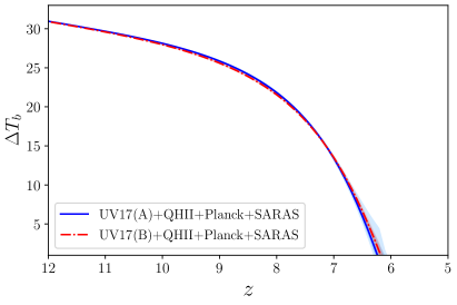
Figure 7: Evolution of the ionization fraction (left panel) and global 21-cm signal at reionization epoch (right panel) obtained using UV17(A)+QHII+Planck+SARAS (blue curve) and UV17(B)+QHII+Planck+SARAS (red dashed line) from the GP reconstruction of the UV luminosity density.

We are now in a position to reconstruct the reionization history profile with the help of these obtained bounds on the parameters $\log_{10}\left\langle f_{\rm esc}\xi_{\rm ion}\right\rangle$, $C_{\rm HII}$, and $\log_{10}\rho_{1-4}$, and by deriving the evolution of the ionization fraction via Eq. (11). Fig. 4 demonstrates the comparison between the reconstructed $Q_{\rm HII}$ using two different data compilations - UV17(A)+QHII+Planck in the left panel vs UV17(B)+QHII+Planck in the right panel. With this reconstructed $Q_{\rm HII}$ profile, we can trace the nature of the 21-cm differential brightness temperature $\Delta T_{b}$, directly employing Eq. (4). Plots for the reconstructed $\Delta T_{b}$ for the UV17(A)+QHII+Planck and UV17(B)+QHII+Planck data sets are shown in the left and right panels of Fig. 5 respectively. As depicted in Figs. 4 and 5, we obtain more or less similar results for the reionization history profile and global signal employing Planck+$Q_{\rm HII}$+ either UV17(A) or UV17(B) data sets. Fixing the clumping factor $C_{\rm HII}$ to a constant value (here $C_{\rm HII}=5$) results in a more precise reconstruction of both $Q_{\rm HII}$ and $\Delta T_{b}$. This feature is apparent from the right panels of Figs. 2 and 3, where we notice a significant reduction of the $\left\langle f_{\rm esc}\xi_{\rm ion}\right\rangle$ parameter space obtained with MCMC analysis. However, one should take it with a pinch of salt, as there is no a priori reason as to why $C_{\rm HII}$ has to take a fixed value, especially when the parameters are not indifferent to a running $C_{\rm HII}$ and hence, the constraints obtained by keeping $C_{\rm HII}$ free should be more acceptable in a conservative approach.

Let us now engage ourselves in investigating the role of the global 21-cm signal on this reconstruction. After plotting the evolution of the 21-cm global signal with best-fit astrophysical parameters from UV17(A)+QHII+Planck and UV17(B)+QHII+Planck data, we create a mock global 21-cm signal $\Delta T_{b}$ vs $z$ data, assuming the instrumental specifications of SARAS. We then redo this entire exercise of learning the reionization history incorporating the SARAS mock data in combination with the remaining UV17(A)/UV17(B), QHII and Planck data sets. Similar to the previous plots, Fig. 6 shows the 2D-confidence contours and 1D-marginalized posteriors for the MCMC parameter space using the joint UV17(A)+QHII+Planck+SARAS and UV17(B)+QHII+Planck+SARAS data sets respectively. In the left panel of Fig. 6, the clumping factor $C_{\rm HII}$ is treated as a free parameter during MCMC, whereas, the right panel shows the case when the value of the clumping factor is kept fixed at $C_{\rm HII}=5$ respectively. Therefore, the inclusion of SARAS data, as shown in Fig. 6, provides much tighter bounds on the astrophysical parameters. In Fig. 7, we plot the evolution of the ionization fraction and global 21-cm signal at the reionization epoch, in the left and right panels, respectively. Our findings show that the reconstructed $Q_{\rm HII}$ and $\Delta T_{b}$ profiles are now further constrained, compared to the previous cases. Thus, one can conclude that although the UV17(A)+QHII+Planck and UV17(B)+QHII+Planck data influence the reionization history and bounds on the astrophysical parameters, the global differential brightness temperature has a more significant impact on constraining these parameters, thereby helping to learn the cosmic reionization history with better precision.

Data sets	$\log_{10}\langle f_{\rm esc}\,\xi_{\rm ion}\rangle$	$C_{\rm HII}$	$\tau_{\rm reio}$	$z_{\rm reio}$	$\Delta z$
UV17(A)+QHII	$24.001_{-0.853}^{+0.405}$	$3.302_{-1.967}^{+3.648}$	$0.054_{-0.0026}^{+0.0038}$	$7.12_{-0.19}^{+0.21}$	$2.21_{-0.19}^{+1.23}$
UV17(A)+QHII, $C_{\rm HII}=5$	$24.417^{+0.032}_{-0.039}$	5	$0.052_{-0.0007}^{+0.0007}$	$7.06_{-0.07}^{+0.05}$	$2.15_{-0.12}^{+0.14}$
UV17(A)+QHII+Planck	$24.192_{-0.411}^{+0.281}$	$4.582_{-2.191}^{+3.197}$	$0.054_{-0.0019}^{+0.0033}$	$7.13_{-0.11}^{+0.19}$	$2.17_{-0.15}^{+0.24}$
UV17(A)+QHII+Planck, $C_{\rm HII}=5$	$24.416_{-0.040}^{+0.034}$	5	$0.052_{-0.0007}^{+0.0007}$	$7.06_{-0.07}^{+0.05}$	$2.15_{-0.13}^{+0.14}$
UV17(A)+QHII+Planck+SARAS	$24.192_{-0.411}^{+0.281}$	$4.582_{-2.191}^{+3.197}$	$0.054_{-0.0019}^{+0.0033}$	$7.13_{-0.11}^{+0.19}$	$2.17_{-0.15}^{+0.24}$
UV17(A)+QHII+Planck+SARAS, $C_{\rm HII}=5$	$24.416_{-0.028}^{+0.027}$	5	$0.052_{-0.0001}^{+0.0001}$	$7.05_{-0.01}^{+0.01}$	$2.13_{-0.05}^{+0.06}$
UV17(B)+QHII	$24.164_{-0.458}^{+0.262}$	$4.760_{-2.485}^{+2.978}$	$0.054_{-0.0015}^{+0.0034}$	$7.13_{-0.10}^{+0.18}$	$2.25_{-0.07}^{+0.20}$
UV17(B)+QHII, $C_{\rm HII}=5$	$24.373_{-0.037}^{+0.026}$	5	$0.053_{-0.0007}^{+0.0005}$	$7.08_{-0.09}^{+0.04}$	$2.24_{-0.04}^{+0.05}$
UV17(B)+QHII+Planck	$24.200_{-0.441}^{+0.247}$	$5.081_{-2.610}^{+3.027}$	$0.054_{-0.0013}^{+0.0031}$	$7.12_{-0.10}^{+0.17}$	$2.25_{-0.08}^{+0.15}$
UV17(B)+QHII+Planck, $C_{\rm HII}=5$	$24.374_{-0.036}^{+0.025}$	5	$0.053_{-0.0007}^{+0.0005}$	$7.08_{-0.08}^{+0.05}$	$2.25_{-0.05}^{+0.06}$
UV17(B)+QHII+Planck+SARAS	$24.273_{-0.141}^{+0.145}$	$6.723_{-1.304}^{+1.933}$	$0.051_{-0.0004}^{+0.0004}$	$6.88_{-0.01}^{+0.01}$	$2.24_{-0.03}^{+0.04}$
UV17(B)+QHII+Planck+SARAS, $C_{\rm HII}=5$	$24.370_{-0.016}^{+0.017}$	5	$0.053_{-0.0001}^{+0.0001}$	$7.07_{-0.01}^{+0.01}$	$2.25_{-0.04}^{+0.03}$

Table 1: Summary of the mean and $1\sigma$ bounds obtained on the astrophysical parameters and reionization history using different data compilations.

The constraints on the astrophysical parameters $\log_{10}\langle f_{\rm esc}\xi_{\rm ion}\rangle,C_{\rm HII}$, optical depth $\tau_{\rm reio}$, reionization redshift $z_{\text{re}}$ and reionization duration $\Delta z$, separately for each individual data compilations explored in the present analysis, are summarized in Table 1. The table shows that the optical depth constraints from all the combinations - UV17+QHII, UV17+QHII+Planck and UV17+QHII+Planck+SARAS align with the 1$\sigma$ optical depth values from Planck 2018 results. Our analysis of reionization duration, $\Delta z$, suggests that a substantial portion of reionization (from 10% to 90% ionization) occurs over approximately 2 units (for Planck+UV17+QHII). The 68% and 95% confidence intervals reveal that the marginalized posterior distribution of $\Delta z$  is slightly skewed when the clumping factor is free to vary during the MCMC. The redshift at which reionization reaches 50% completion, denoted as $z_{\text{re}}$, is found to be approximately 7 for all the above-mentioned data combinations. The table shows that the mean value of $\log_{10}\langle f_{\rm esc}\xi_{\rm ion}\rangle$ parameter is approximately 24 units from all combinations of data sets. With the inclusion of SARAS data and keeping $C_{\rm HII}$ fixed, the 1$\sigma$ bounds on the $\log_{10}\langle f_{\rm esc}\xi_{\rm ion}\rangle$ parameter are significantly constrained. The $C_{\rm HII}$ parameter takes different values for different data set combinations. The 1$\sigma$ bound on this parameter improves with the UV17(B)+QHII+Planck+SARAS data set combination.

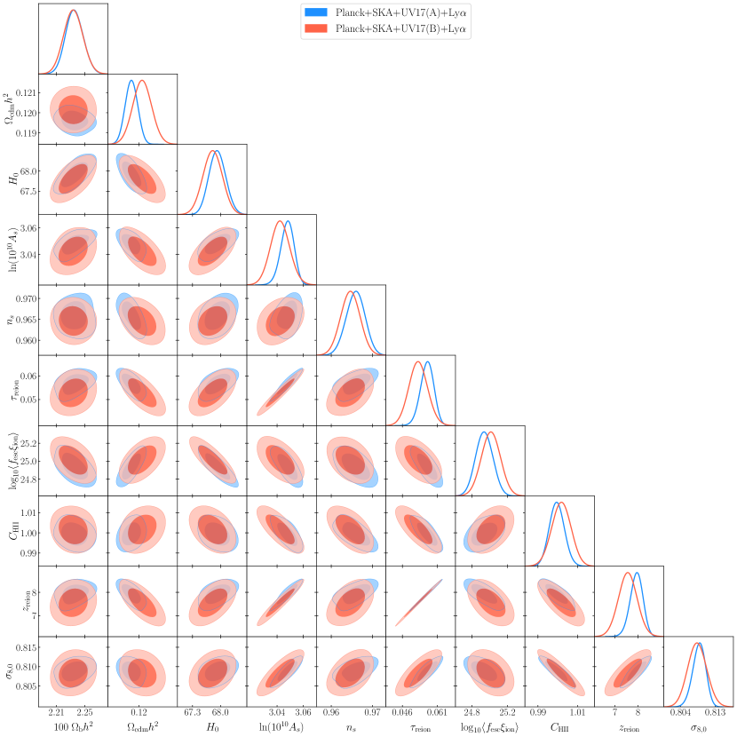
Figure 8: Forecasting the reionization power spectrum of 6 $\Lambda$CDM parameters with 2 astrophysical parameters: ionization efficiency and clumping factor, using the Planck+SKA+Ly$\alpha$+UV17(A) data sets and the Planck+SKA+Ly$\alpha$+UV17(B) data sets. Here for this forecast and MCMC analysis, we have used fake Planck realistic data. The analysis is undertaken using the mean reconstructed $Q_{\rm HII}$ function, without incorporating the errors.

Our final target is to explore the prospects of the upcoming 21-cm mission SKA in simultaneously inferring the 2 astrophysical + 6 cosmological parameters. For this, we make use of the reconstructed reionization history and compute the 21-cm power spectrum during the reionization epoch with a conservative approach, employing Eq. (6). Further, we modify the Boltzmann solver code CLASS in order to accommodate our reconstructed reionization history (as opposed to using baseline Planck $\tanh$ reionization model), as explained in Sec. 4.2. The underlying cosmological model was set to the standard 6-parameter $\Lambda$CDM framework. Following the prescription given by Sprenger et al. (2019), we generate mock catalogues for the future SKA mission in the reionization era between redshift $z\approx 6-12$, from the simulated Planck realistic data, utilizing the fake_planck_realistic likelihood in MontePython (hereafter referred to as Planck), adopting the fiducial values of the cosmological parameters as $w_{\rm b}=0.02237$, $w_{\rm cdm}=0.12010$, $\ln[10^{10}A_{s}]=3.0447$, $n_{s}=0.9659$, $H_{0}=67.8$ km Mpc^-1 s^-1, $\tau_{\rm reio}=0.0543$, consistent with Planck18 data (Planck Collaboration et al., 2020). Finally, we undertake a Bayesian MCMC analysis to forecast the 6 cosmological and 2 astrophysical parameters using the MontePython code. We adopt uniform priors for all parameters as: $100~{}\Omega_{\rm b}h^{2}\in\mathcal{U}[0.05,10]$, $\Omega_{\rm c}h^{2}\in\mathcal{U}[0.01,0.99]$, $H_{0}\in\mathcal{U}[50,100]$, $n_{s}\in\mathcal{U}[0.5,1.5]$, $\tau_{\rm reion}\in\mathcal{U}[0.004,0.2]$, $\ln\left(10^{10}A_{s}\right)\in\mathcal{U}[1,5]$, $\left\langle f_{\rm esc}\xi_{\rm ion}\right\rangle\in\mathcal{U}[20,30]$, and an upper bound on $C_{\rm HII}\leq 10$ respectively. The resulting 2D-confidence contours and 1D-marginalized posteriors for the Planck+SKA+Ly$\alpha$+UV17(A) and Planck+SKA+Ly$\alpha$+UV17(B) data sets have been presented in Fig. 8, which also helps us in easy comparison between the two data sets. Table 2 presents the mean and $1\sigma$ bound on the astrophysical and cosmological parameters obtained from this analysis. Besides, we also show the results for two derived parameters $z_{\rm reion}$ and $\sigma_{8,0}$.

Parameters	$\tanh$ reionization model	GP reconstructed reionization model
	Planck 2018 TT,TE,EE + lowE	Planck+SKA+Ly$\alpha$+UV17(A)	Planck+SKA+Ly$\alpha$+UV17(B)
$\log_{10}\langle f_{\rm esc}\,\xi_{\rm ion}\rangle$	$23-500$	$24.94_{-0.1}^{+0.088}$	$24.99_{-0.08}^{+0.07}$
$C_{\rm HII}$	$1-10$	$0.9995_{-0.0036}^{+0.0035}$	$1.001_{-0.0047}^{+0.0044}$
$100\,\Omega_{\rm b}h^{2}$	$2.236\pm 0.015$	$2.235_{-0.013}^{+0.0095}$	$2.239_{-0.002}^{+0.008}$
$\Omega_{\rm cdm}h^{2}$	$0.1202\pm 0.0014$	$0.1196_{-0.00031}^{+0.00033}$	$0.12_{-0.005}^{+0.005}$
$H_{0}$	$67.27\pm 0.60$	$67.92_{-0.21}^{+0.19}$	$67.88_{-0.3}^{+0.21}$
$\ln\left(10^{10}A_{s}\right)$	$3.045\pm 0.016$	$3.048_{-0.0044}^{+0.0053}$	$3.045_{-0.0064}^{+0.0056}$
$n_{s}$	$0.9649\pm 0.0044$	$0.9658_{-0.0019}^{+0.0023}$	$0.9644_{-0.002}^{+0.003}$
$\tau_{\rm reio}$	$0.0544_{-0.0081}^{+0.0070}$	$0.0566_{-0.0025}^{+0.003}$	$0.05386_{-0.0057}^{+0.005}$
$100\,\theta_{s}$	$1.04077\pm 0.00047$	$1.044_{-0.00024}^{+0.00027}$	$1.044_{-0.00038}^{+0.00028}$
$z_{\rm reio}$	$7.68\pm 0.79$	$7.93_{-0.26}^{+0.28}$	$7.66_{-0.367}^{+0.289}$
$\sigma_{8}$	$0.8120\pm 0.0073$	$0.8088_{-0.0013}^{+0.0019}$	$0.8088_{-0.002}^{+0.0015}$

Table 2: Summary of the mean and $1\sigma$ bounds obtained on the astrophysical and cosmological parameters using the $\tanh$ model of reionization for Planck TT + lowE data (Planck Collaboration et al., 2020) and using the reconstructed reionization history for the Planck+SKA+Ly$\alpha$+UV17(A) and UV17(B) data sets.

A comparison of the results presented in Table 1 and Table 2 for the two key cosmological parameters $\tau_{\rm reion}$ and $z_{\rm reion}$, as well as the two astrophysical parameters $C_{\rm HII}$ and $\langle f_{\rm esc}\xi_{\rm ion}\rangle$ is in order. Based on the power spectrum analysis, we achieve tighter $1\sigma$ bounds on the astrophysical parameters $\log_{10}\langle f_{\rm esc}\,\xi_{\rm ion}\rangle$ and $C_{\rm HII}$ compared to the results in Table 1. The parameter $z_{\rm reio}$, which denotes the redshift at which 50% ionization is complete, shows a relatively higher value from the power spectrum analysis (somewhat akin to tanh reionization model) than from the global signal reconstruction analysis. However, a crucial difference between the two analyses needs to be kept in mind. In the power spectrum analysis, we considered the full fake Planck realistic data and ran MCMC for the 6 cosmological parameters along with the astrophysical parameters. In contrast, for the global signal reconstruction, we used the Planck optical depth measurement and ran MCMC for the astrophysical parameters only. This difference may have shown up as the slight difference in the $z_{\rm reio}$ values estimated from the two analyses and one should rely more on the “all parameters open” case than the other one.

Further, for comparison with the baseline reionization model, we also present the results for the 6-parameter $\Lambda$CDM with $\tanh$ reionization model in Table 2, which shows that our obtained values of $\tau_{\rm reio}$, $z_{\rm reion}$, $H_{0}$, $\sigma_{8}$, and other cosmological parameters using the GP reconstrued reionization history are well consistent with the Planck 2018 + baseline model. On top of that, both of the astrophysical parameters $C_{\rm HII}$ and $\langle f_{\rm esc}\xi_{\rm ion}\rangle$ prefer values closer to the lower bounds of the tanh model. This happens in spite of choosing a wide prior range for both of them. We observe that the mean values of $H_{0}$ remain almost unaffected and lie close to the baseline Planck values, similar to Chatterjee et al. (2021). However, the mean value of $\sigma_{8}$ slightly decreases when changing the reionization history. This feature is similar to previous observations made in Fig. 4 of Hazra et al. (2020) using non-parametric nodal reconstruction, nonetheless that the astrophysical parameters were kept fixed to $\log_{10}\left\langle f_{\rm esc}\xi_{\rm ion}\right\rangle$ = 24.85 (Ishigaki et al., 2015) and $C_{\rm HII}\leq 3$, focusing on examining how the reconstructed model affects the constraints on the cosmological parameters. Paoletti et al. (2021) extended this exercise by varying the reionization astrophysical parameters simultaneously with the cosmological parameters using Planck+UV17+QHII data sets. The constraints obtained on the key parameters, such as $\log_{10}\left\langle f_{\rm esc}\xi_{\rm ion}\right\rangle$ and $\tau_{\rm reion}$ in Table 3 & 4 of Paoletti et al. (2021) are consistent with our results, shown in Table 2. We believe the above consistency checks make the reconstruction technique a robust learning process and the inferences on the astrophysical parameters obtained therefrom are quite reliable that can be used for future analysis.

6 Concluding Remarks

In this article, we have investigated how GPR can help to better understand the history of reionization and related astrophysical parameters during this period. We have trained the GP algorithm for model-independent reconstruction of the UV luminosity density function using UV17(A) and UV17(B) data, which is then combined with the Planck optical depth and QHII Lyman-$\alpha$ data sets to undertake a non-parametric reconstruction of the reionization history. For a robust analysis, we allowed the parameters of the logarithmic double power law and kernel hyperparameters to vary freely during GP training, expanding upon previous literature (Ishigaki et al., 2018; Hazra et al., 2020; Adak et al., 2024), and found our results to be consistent. The clumping factor was kept free to vary, rather than being fixed to specific values like 3 (Hazra et al., 2020) or 5 (Adak et al., 2024), as there is no a priori reason to rule out redshift variations in $C_{\rm HII}$. This approach allowed for a comparative analysis of the roles of astrophysical parameters in deriving the reionization history.

We extended our analysis to explore previously unexplored applications of GPR in reionization. This involved separately considering the global 21-cm signal and the 21-cm power spectrum to investigate their roles in learning the astrophysical parameters and reionization history. To study the effect of the global 21-cm signal, we have trained the GPR algorithm using the mock data of SARAS and found that the inclusion of SARAS in the reconstruction analysis significantly improves the bounds on the astrophysical parameters during reionization. In the final part, we have presented the 21-cm power spectrum analysis based on the reconstructed reionization history, by making modifications to the Boltzmann solver code CLASS and MCMC code MontePython. Our findings indicate that the power spectrum analysis for the modified reionization history with future SKA will help improve the bounds on six cosmological parameters and two astrophysical parameters. Additionally, both of the astrophysical parameters prefer values closer to the lower bounds of the baseline tanh reionization model. This leads us to believe that our GPR-based reconstruction technique works very well in the context of reionization, both for global 21-cm signal and for 21-cm power spectrum, in combination with other relevant data sets. The constraints on astrophysical parameters derived from this method are reliable and can be used in future reionization studies.

However, our reconstruction analysis can be generalized in different ways. The power spectrum analysis presented here is based on the Eq. (6) and does not take into account the redshift evolution of $\log_{10}\langle f_{\rm esc}\xi_{\rm ion}\rangle$ and $C_{\rm HII}$ parameters. A more rigorous analysis will involve reionization simulation for estimating the actual bounds on the astrophysical parameters and possible reflections on SKA (Mangena et al., 2020). Further, our analysis is based only on the $\Lambda$CDM model; as our future goal, we will explore beyond-$\Lambda$CDM models and investigate their impact on the reionization period. For reconstruction purposes, the kinetic Sunyaev-Zeldovich data (Jain et al., 2024) can also be added on top of current data sets and the possible consequences can be investigated. Lastly, while we have utilized the GPR technique as an ML tool for learning, future investigations will explore various ML techniques (Sohn et al., 2024; Gómez-Vargas et al., 2023; Shah et al., 2024; Mukherjee et al., 2024a) for training and testing in the context of reionization. We look forward to pursuing these avenues in future work.

emcee (Foreman-Mackey et al., 2013), CLASS (Blas et al., 2011), MontePython (Audren et al., 2013; Brinckmann & Lesgourgues, 2019)

References

- Abdurashidova et al. (2022) Abdurashidova, Z., et al. 2022, Astrophys. J., 924, 51, doi: 10.3847/1538-4357/ac2ffc
- Adak et al. (2024) Adak, D., Hazra, D. K., Mitra, S., & Krishak, A. 2024. https://arxiv.org/abs/2405.10180
- Atek et al. (2024) Atek, H., Labbé, I., Furtak, L. J., et al. 2024, Nature, 626, 975, doi: 10.1038/s41586-024-07043-6
- Audren et al. (2013) Audren, B., Lesgourgues, J., Benabed, K., & Prunet, S. 2013, JCAP, 1302, 001, doi: 10.1088/1475-7516/2013/02/001
- Barkana & Loeb (2001) Barkana, R., & Loeb, A. 2001, Phys. Rept., 349, 125, doi: 10.1016/S0370-1573(01)00019-9
- Blas et al. (2011) Blas, D., Lesgourgues, J., & Tram, T. 2011, JCAP, 07, 034, doi: 10.1088/1475-7516/2011/07/034
- Bolton et al. (2011) Bolton, J. S., Haehnelt, M. G., Warren, S. J., et al. 2011, MNRAS, 416, L70, doi: 10.1111/j.1745-3933.2011.01100.x
- Bouwens et al. (2023) Bouwens, R., Illingworth, G., Oesch, P., et al. 2023, Mon. Not. Roy. Astron. Soc., 523, 1009, doi: 10.1093/mnras/stad1014
- Bouwens et al. (2015a) Bouwens, R. J., Illingworth, G. D., Oesch, P. A., et al. 2015a, Astrophys. J., 811, 140, doi: 10.1088/0004-637X/811/2/140
- Bouwens et al. (2017) Bouwens, R. J., Oesch, P. A., Illingworth, G. D., Ellis, R. S., & Stefanon, M. 2017, Astrophys. J., 843, 129, doi: 10.3847/1538-4357/aa70a4
- Bouwens et al. (2015b) Bouwens, R. J., et al. 2015b, Astrophys. J., 803, 34, doi: 10.1088/0004-637X/803/1/34
- Bouwens et al. (2021) Bouwens, R. J., Oesch, P. A., Stefanon, M., et al. 2021, AJ, 162, 47, doi: 10.3847/1538-3881/abf83e
- Brinckmann & Lesgourgues (2019) Brinckmann, T., & Lesgourgues, J. 2019, Phys. Dark Univ., 24, 100260, doi: 10.1016/j.dark.2018.100260
- Cain et al. (2021) Cain, C., D’Aloisio, A., Gangolli, N., & Becker, G. D. 2021, ApJ, 917, L37, doi: 10.3847/2041-8213/ac1ace
- Chatterjee et al. (2021) Chatterjee, A., Choudhury, T. R., & Mitra, S. 2021, Mon. Not. Roy. Astron. Soc., 507, 2405, doi: 10.1093/mnras/stab2316
- Choudhury (2009) Choudhury, T. R. 2009, Current Science, 97, 841, doi: 10.48550/arXiv.0904.4596
- Choudhury & Ferrara (2005) Choudhury, T. R., & Ferrara, A. 2005, Mon. Not. Roy. Astron. Soc., 361, 577, doi: 10.1111/j.1365-2966.2005.09196.x
- Das et al. (2018) Das, S., Mondal, R., Rentala, V., & Suresh, S. 2018, J. Cosmology Astropart. Phys, 2018, 045, doi: 10.1088/1475-7516/2018/08/045
- Davies et al. (2018) Davies, F. B., et al. 2018, Astrophys. J., 864, 142, doi: 10.3847/1538-4357/aad6dc
- Dayal & Ferrara (2018) Dayal, P., & Ferrara, A. 2018, Phys. Rept., 780-782, 1, doi: 10.1016/j.physrep.2018.10.002
- de Lera Acedo et al. (2015) de Lera Acedo, E., Razavi-Ghods, N., Troop, N., Drought, N., & Faulkner, A. J. 2015, Experimental Astronomy, 39, 567, doi: 10.1007/s10686-015-9439-0
- de Oliveira-Costa et al. (2008) de Oliveira-Costa, A., Tegmark, M., Gaensler, B. M., et al. 2008, Mon. Not. Roy. Astron. Soc., 388, 247, doi: 10.1111/j.1365-2966.2008.13376.x
- Dewdney & Braun (2016) Dewdney, P. E., & Braun, R. 2016, SKA Organisation, 2, 1
- Dey et al. (2023a) Dey, A., Paul, A., & Pal, S. 2023a, Mon. Not. Roy. Astron. Soc., 524, 100, doi: 10.1093/mnras/stad1838
- Dey et al. (2023b) —. 2023b, Mon. Not. Roy. Astron. Soc., 527, 790, doi: 10.1093/mnras/stad3180
- Ellis et al. (2013) Ellis, R. S., et al. 2013, Astrophys. J. Lett., 763, L7, doi: 10.1088/2041-8205/763/1/L7
- Finkelstein et al. (2019) Finkelstein, S. L., D’Aloisio, A., Paardekooper, J.-P., et al. 2019, ApJ, 879, 36, doi: 10.3847/1538-4357/ab1ea8
- Finlator et al. (2012) Finlator, K., Oh, S. P., Ozel, F., & Dave, R. 2012, Mon. Not. Roy. Astron. Soc., 427, 2464, doi: 10.1111/j.1365-2966.2012.22114.x
- Foreman-Mackey et al. (2013) Foreman-Mackey, D., Hogg, D. W., Lang, D., & Goodman, J. 2013, Publ. Astron. Soc. Pac., 125, 306, doi: 10.1086/670067
- Furlanetto et al. (2006) Furlanetto, S., Oh, S. P., & Briggs, F. 2006, Phys. Rept., 433, 181, doi: 10.1016/j.physrep.2006.08.002
- Gerardi et al. (2019) Gerardi, F., Martinelli, M., & Silvestri, A. 2019, JCAP, 07, 042, doi: 10.1088/1475-7516/2019/07/042
- Gómez-Vargas et al. (2023) Gómez-Vargas, I., Andrade, J. B., & Vázquez, J. A. 2023, Phys. Rev. D, 107, 043509, doi: 10.1103/PhysRevD.107.043509
- Gorce et al. (2018) Gorce, A., Douspis, M., Aghanim, N., & Langer, M. 2018, Astron. Astrophys., 616, A113, doi: 10.1051/0004-6361/201629661
- Greig et al. (2017) Greig, B., Mesinger, A., Haiman, Z., & Simcoe, R. A. 2017, Mon. Not. Roy. Astron. Soc., 466, 4239, doi: 10.1093/mnras/stw3351
- Harikane et al. (2022) Harikane, Y., Ono, Y., Ouchi, M., et al. 2022, ApJS, 259, 20, doi: 10.3847/1538-4365/ac3dfc
- Harikane et al. (2023) Harikane, Y., Ouchi, M., Oguri, M., et al. 2023, ApJS, 265, 5, doi: 10.3847/1538-4365/acaaa9
- Hazra et al. (2020) Hazra, D. K., Paoletti, D., Finelli, F., & Smoot, G. F. 2020, Phys. Rev. Lett., 125, 071301, doi: 10.1103/PhysRevLett.125.071301
- Hirata (2006) Hirata, C. M. 2006, Mon. Not. Roy. Astron. Soc., 367, 259, doi: 10.1111/j.1365-2966.2005.09949.x
- Iliev et al. (2006) Iliev, I. T., Mellema, G., Pen, U.-L., et al. 2006, Mon. Not. Roy. Astron. Soc., 369, 1625, doi: 10.1111/j.1365-2966.2006.10502.x
- Inoue et al. (2014) Inoue, A. K., Shimizu, I., & Iwata, I. 2014, Mon. Not. Roy. Astron. Soc., 442, 1805, doi: 10.1093/mnras/stu936
- Ishigaki et al. (2015) Ishigaki, M., Kawamata, R., Ouchi, M., et al. 2015, ApJ, 799, 12, doi: 10.1088/0004-637X/799/1/12
- Ishigaki et al. (2018) —. 2018, ApJ, 854, 73, doi: 10.3847/1538-4357/aaa544
- Jain et al. (2024) Jain, D., Choudhury, T. R., Raghunathan, S., & Mukherjee, S. 2024, Mon. Not. Roy. Astron. Soc., 530, 35, doi: 10.1093/mnras/stae748
- Katz et al. (2023) Katz, H., et al. 2023, Mon. Not. Roy. Astron. Soc., 518, 270, doi: 10.1093/mnras/stac3019
- Krishak & Hazra (2021) Krishak, A., & Hazra, D. K. 2021, Astrophys. J., 922, 95, doi: 10.3847/1538-4357/ac3251
- Kuhlen & Faucher-Giguere (2012) Kuhlen, M., & Faucher-Giguere, C. A. 2012, Mon. Not. Roy. Astron. Soc., 423, 862, doi: 10.1111/j.1365-2966.2012.20924.x
- Kulkarni et al. (2019) Kulkarni, G., Keating, L. C., Haehnelt, M. G., et al. 2019, MNRAS, 485, L24, doi: 10.1093/mnrasl/slz025
- Lotz et al. (2017) Lotz, J. M., et al. 2017, Astrophys. J., 837, 97, doi: 10.17909/T9KK5N
- Lotz et al. (2017) Lotz, J. M., Koekemoer, A., Coe, D., et al. 2017, ApJ, 837, 97, doi: 10.3847/1538-4357/837/1/97
- Madau et al. (1999) Madau, P., Haardt, F., & Rees, M. J. 1999, ApJ, 514, 648, doi: 10.1086/306975
- Madau et al. (1997) Madau, P., Meiksin, A., & Rees, M. J. 1997, Astrophys. J., 475, 429, doi: 10.1086/303549
- Mangena et al. (2020) Mangena, T., Hassan, S., & Santos, M. G. 2020, Mon. Not. Roy. Astron. Soc., 494, 600, doi: 10.1093/mnras/staa750
- Mason et al. (2019) Mason, C. A., Fontana, A., Treu, T., et al. 2019, MNRAS, 485, 3947, doi: 10.1093/mnras/stz632
- McGreer et al. (2015) McGreer, I. D., Mesinger, A., & D’Odorico, V. 2015, MNRAS, 447, 499, doi: 10.1093/mnras/stu2449
- McLeod et al. (2016) McLeod, D. J., McLure, R. J., & Dunlop, J. S. 2016, MNRAS, 459, 3812, doi: 10.1093/mnras/stw904
- McLure et al. (2013) McLure, R. J., et al. 2013, Mon. Not. Roy. Astron. Soc., 432, 2696, doi: 10.1093/mnras/stt627
- McQuinn et al. (2008) McQuinn, M., Lidz, A., Zaldarriaga, M., Hernquist, L., & Dutta, S. 2008, MNRAS, 388, 1101, doi: 10.1111/j.1365-2966.2008.13271.x
- Mesinger et al. (2016) Mesinger, A., Greig, B., & Sobacchi, E. 2016, Mon. Not. Roy. Astron. Soc., 459, 2342, doi: 10.1093/mnras/stw831
- Mitra & Chatterjee (2023) Mitra, S., & Chatterjee, A. 2023, Mon. Not. Roy. Astron. Soc., 523, L35, doi: 10.1093/mnrasl/slad055
- Morandi & Barkana (2012) Morandi, A., & Barkana, R. 2012, MNRAS, 424, 2551, doi: 10.1111/j.1365-2966.2012.21240.x
- Mortlock et al. (2011) Mortlock, D. J., Warren, S. J., Venemans, B. P., et al. 2011, Nature, 474, 616, doi: 10.1038/nature10159
- Muñoz et al. (2024) Muñoz, J. B., Mirocha, J., Chisholm, J., Furlanetto, S. R., & Mason, C. 2024. https://arxiv.org/abs/2404.07250
- Mukherjee (2022) Mukherjee, P. 2022, PhD thesis, IISER, Kolkata. https://arxiv.org/abs/2207.07857
- Mukherjee et al. (2024a) Mukherjee, P., Dialektopoulos, K. F., Levi Said, J., & Mifsud, J. 2024a. https://arxiv.org/abs/2402.10502
- Mukherjee et al. (2024b) Mukherjee, P., Shah, R., Bhaumik, A., & Pal, S. 2024b, Astrophys. J., 960, 61, doi: 10.3847/1538-4357/ad055f
- Oesch et al. (2018) Oesch, P. A., Bouwens, R. J., Illingworth, G. D., Labbé, I., & Stefanon, M. 2018, ApJ, 855, 105, doi: 10.3847/1538-4357/aab03f
- Ono et al. (2012) Ono, Y., Ouchi, M., Mobasher, B., et al. 2012, ApJ, 744, 83, doi: 10.1088/0004-637X/744/2/83
- Paoletti et al. (2021) Paoletti, D., Hazra, D. K., Finelli, F., & Smoot, G. F. 2021, Phys. Rev. D, 104, 123549, doi: 10.1103/PhysRevD.104.123549
- Paoletti et al. (2024) —. 2024. https://arxiv.org/abs/2405.09506
- Patra et al. (2013) Patra, N., Subrahmanyan, R., Raghunathan, A., & Udaya Shankar, N. 2013, Experimental Astronomy, 36, 319, doi: 10.1007/s10686-013-9336-3
- Pawlik et al. (2009) Pawlik, A. H., Schaye, J., & van Scherpenzeel, E. 2009, Mon. Not. Roy. Astron. Soc., 394, 1812, doi: 10.1111/j.1365-2966.2009.14486.x
- Planck Collaboration et al. (2020) Planck Collaboration, Aghanim, N., Akrami, Y., et al. 2020, A&A, 641, A6, doi: 10.1051/0004-6361/201833910
- Price et al. (2016) Price, L. C., Trac, H., & Cen, R. 2016. https://arxiv.org/abs/1605.03970
- Pritchard & Loeb (2012) Pritchard, J. R., & Loeb, A. 2012, Rept. Prog. Phys., 75, 086901, doi: 10.1088/0034-4885/75/8/086901
- Rasmussen & Williams (2006) Rasmussen, C. E., & Williams, C. K. I. 2006, Gaussian Processes for Machine Learning (The MIT Press)
- Robertson (2021) Robertson, B. E. 2021, Annual Review of Astronomy and Astrophysics, doi: 10.1146/annurev-astro-120221-044656
- Robertson et al. (2013) Robertson, B. E., et al. 2013, Astrophys. J., 768, 71, doi: 10.1088/0004-637X/768/1/71
- Sarkar et al. (2016) Sarkar, A., Mondal, R., Das, S., et al. 2016, JCAP, 04, 012, doi: 10.1088/1475-7516/2016/04/012
- Schenker et al. (2014) Schenker, M. A., Ellis, R. S., Konidaris, N. P., & Stark, D. P. 2014, ApJ, 795, 20, doi: 10.1088/0004-637X/795/1/20
- Schenker et al. (2013) Schenker, M. A., et al. 2013, Astrophys. J., 768, 196, doi: 10.1088/0004-637X/768/2/196
- Schroeder et al. (2013) Schroeder, J., Mesinger, A., & Haiman, Z. 2013, Mon. Not. Roy. Astron. Soc., 428, 3058, doi: 10.1093/mnras/sts253
- Seikel et al. (2012) Seikel, M., Clarkson, C., & Smith, M. 2012, JCAP, 06, 036, doi: 10.1088/1475-7516/2012/06/036
- Shafieloo et al. (2012) Shafieloo, A., Kim, A. G., & Linder, E. V. 2012, Phys. Rev. D, 85, 123530, doi: 10.1103/PhysRevD.85.123530
- Shah et al. (2023) Shah, R., Bhaumik, A., Mukherjee, P., & Pal, S. 2023, JCAP, 06, 038, doi: 10.1088/1475-7516/2023/06/038
- Shah et al. (2024) Shah, R., Saha, S., Mukherjee, P., Garain, U., & Pal, S. 2024, ApJS 273, 27, doi: 10.3847/1538-4365/ad5558
- Simmonds et al. (2024) Simmonds, C., Tacchella, S., Hainline, K., et al. 2024, MNRAS, 527, 6139, doi: 10.1093/mnras/stad3605
- Singh et al. (2018) Singh, S., et al. 2018, Astrophys. J., 858, 54, doi: 10.3847/1538-4357/aabae1
- Sohn et al. (2024) Sohn, W., Shafieloo, A., & Hazra, D. K. 2024, JCAP, 03, 056, doi: 10.1088/1475-7516/2024/03/056
- Sprenger et al. (2019) Sprenger, T., Archidiacono, M., Brinckmann, T., Clesse, S., & Lesgourgues, J. 2019, JCAP, 02, 047, doi: 10.1088/1475-7516/2019/02/047
- Tegmark & Zaldarriaga (2009) Tegmark, M., & Zaldarriaga, M. 2009, Phys. Rev. D, 79, 083530, doi: 10.1103/PhysRevD.79.083530
- Tilvi et al. (2014) Tilvi, V., Papovich, C., Finkelstein, S. L., et al. 2014, ApJ, 794, 5, doi: 10.1088/0004-637X/794/1/5
- Totani et al. (2006) Totani, T., Kawai, N., Kosugi, G., et al. 2006, PASJ, 58, 485, doi: 10.1093/pasj/58.3.485
- van Haarlem et al. (2013) van Haarlem, M. P., Wise, M. W., Gunst, A. W., et al. 2013, A&A, 556, A2, doi: 10.1051/0004-6361/201220873
- Viel et al. (2013) Viel, M., Becker, G. D., Bolton, J. S., & Haehnelt, M. G. 2013, Phys. Rev. D, 88, 043502, doi: 10.1103/PhysRevD.88.043502
- Wouthuysen (1952) Wouthuysen, S. A. 1952, AJ, 57, 31, doi: 10.1086/106661
- Yu et al. (2012) Yu, Y.-W., Cheng, K. S., Chu, M. C., & Yeung, S. 2012, J. Cosmology Astropart. Phys, 2012, 023, doi: 10.1088/1475-7516/2012/07/023
- Zaldarriaga et al. (2004) Zaldarriaga, M., Furlanetto, S. R., & Hernquist, L. 2004, Astrophys. J., 608, 622, doi: 10.1086/386327