6.5pt0.5pt []Supplemental_Material

Fermion Masses and Mixings in String Theory with Dirac Neutrinos

Abstract

We examine the most realistic class of models among the 33 candidates in the complete landscape of supersymmetric Pati-Salam models arising from intersecting D6-branes on a $\mathbbm{T}^{6}/(\mathbbm{Z}_{2}\times\mathbbm{Z}_{2})$ orientifold in type IIA string theory. The class is characterized by twelve Higgs from the $\mathcal{N}=2$ sector that precisely account for the Standard Model fermion masses and mixings without Wilson fluxes. Notably, there is a natural prediction of Dirac neutrino-masses with normal ordering $(50.4,~{}10.5,~{}6.1)$ meV consistent with both experimental constraints and swampland bounds.

Introduction – Standard Model (SM) fermions appear in chiral representations of the gauge group $\textrm{SU}(3)_{C}\times\textrm{SU}(2)_{L}\times\textrm{U}(1)_{Y}$. Intersecting D6-branes in type IIA string theory provide a natural mechanism to realize chiral fermions at D6-brane intersections [1]. Family replication results from multiple intersections of D6-branes that fill four-dimensional spacetime and extend into three compact dimensions. The volumes of the cycles wrapped by D-branes determine the four-dimensional gauge couplings, while the total internal volume yields the gravitational coupling. Yukawa couplings arise from open world-sheet instantons, specifically the triangular worldsheets stretched between intersections where fields involved in the cubic coupling reside. These instanton effects are suppressed by $\exp(-A_{ijk}T)$, where $A_{ijk}$ is the area of the triangle bounded by intersections $\{i,j,k\}$ and $T$ is the string tension [2]. This exponential suppression explains the fermion mass hierarchies and mixings. However, embedding the Standard Model (SM) in a Calabi-Yau compactification with three families of chiral fermions and achieving correct fermion mass hierarchies and mixings in a positively curved (de Sitter) universe with stabilized moduli has been a challenge.

In grand unified models, we relax the requirement of stable de Sitter and impose minimal supersymmetry for computational control. Realistic Yukawa textures with three families favors direct products of unitary gauge groups over the simple unitary group. And the K-theory conditions [3, 4], being mod 4, are more easily satisfied for $\textrm{U}(2N)$ with $N\in\mathbbm{Z}$. Consequently, the left-right symmetric Pati-Salam group, $\textrm{SU}(4)_{C}\times\textrm{SU}(2)_{L}\times\textrm{SU}(2)_{R}$, emerges as the most promising choice for realistic models. The rules to construct supersymmetric Pati-Salam models on a $\mathbbm{T}^{6}/(\mathbbm{Z}_{2}\times\mathbbm{Z}_{2})$ orientifold from intersecting D6-branes with the requirement of $\mathcal{N}=1$ supersymmetry, tadpole cancellation and the K-theory constraints were outlined in [6, 7, 8]. Similar construction is employed in recent works [9, 10, 11, 12, 13]. In ref. [14] the complete landscape of consistent three-family supersymmetric Pati-Salam models from intersecting D6-branes on a $\mathbbm{T}^{6}/(\mathbbm{Z}_{2}\times\mathbbm{Z}_{2})$ orientifold was fully mapped, comprising of only 33 distinct models. The viable models with realistic Yukawas split into classes of either 6, 9 or 12 Higgs fields from $\mathcal{N}=2$ sector [15].

Recent evidence from the swampland program [16], particularly from the non-SUSY AdS instability conjecture [17] and the light fermion conjecture [18, 19], building on the earlier work of [20, 21] suggests that without additional chiral fermions with tiny masses, neutrinos must be of Dirac-type together with a bound on the lightest neutrino mass given by the cosmological constant scale as, $m_{\nu}^{\rm lightest}\lesssim\Lambda^{1/4}$ [22, 23, 24, 25]. The 3D Casimir energy of the SM compactified on a circle receives a positive contribution from the lightest neutrino, which is necessary to avoid unstable non-supersymmetric AdS vacua. This constraint is only satisfied for Dirac neutrinos, which carry 4 degrees of freedom, unlike Majorana neutrinos, which only have 2 and cannot compensate for the 4 bosonic degrees of freedom from the photon and the graviton. This also avoids the inevitable lepton-number violations in the Majorana case. Hence, it is crucial in string theory to generate tiny Dirac Yukawa couplings while keeping the other Yukawa couplings and SM gauge couplings unsuppressed. Previous attempts to generate Dirac neutrino masses in intersecting D-branes primarily focused on Euclidean D2-brane instantons within local models [26, 27, 28]. For a recent survey on this issue, see Ref. [29].

Table 1: D6-brane configurations and intersection numbers of Model 22, and its MSSM gauge coupling relation is $g^{2}_{a}=\frac{5}{6}g^{2}_{b}=\frac{11}{6}g^{2}_{c}=\frac{11}{8}(\frac{5}{3}g^{2}_{Y})=\frac{8}{7\sqrt{3}}\sqrt[4]{2}\,5^{3/4}\,\pi\,e^{\phi_{4}}$. Model 22-dual is obtained by exchanging $b\leftrightarrow c$ with the gauge coupling relation $g^{2}_{a}=\frac{11}{6}g^{2}_{b}=\frac{5}{6}g^{2}_{c}=\frac{25}{28}(\frac{5}{3}g^{2}_{Y})=\frac{8}{7\sqrt{3}}\,\sqrt[4]{2}\,5^{3/4}\,\pi\,e^{\phi_{4}}$.

$\begin{array}[]{|c|c|c|c|c|c|c|c|c|c|}\hline\cr\vrule\lx@intercol\hfil\text{Model~{}\hyperref@@ii[model22]{22}}\hfil\lx@intercol\vrule\lx@intercol&\lx@intercol\hfil{\textrm{U}(4)_{C}\times\textrm{U}(2)_{L}\times\textrm{U}(2)_{R}\times\textrm{USp}(2)}\hfil\lx@intercol\vrule\lx@intercol\\ \hline\cr\hline\cr\rm{stack}&N&(n^{1},l^{1})\times(n^{2},l^{2})\times(n^{3},l^{3})&n_{\yng(2)}&n_{\yng(1,1)}&b&b^{\prime}&c&c^{\prime}&3\\ \hline\cr a&8&(1,-1)\times(1,0)\times(1,1)&0&0&3&0&-3&0&0\\ b&4&(-2,5)\times(0,1)\times(-1,1)&3&-3&\text{-}&\text{-}&0&-8&2\\ c&4&(2,1)\times(1,1)\times(1,-1)&2&6&\text{-}&\text{-}&\text{-}&\text{-}&2\\ \hline\cr 3&2&(0,-1)\times(1,0)\times(0,2)&\lx@intercol\hfil~{}\beta^{g}_{3}=-2,\hfil\lx@intercol\vrule\lx@intercol\\ &&&\lx@intercol\hfil\chi_{1}=\sqrt{\frac{2}{5}},~{}\chi_{2}=\frac{\sqrt{\frac{5}{2}}}{6},{}\hfil\lx@intercol\vrule\lx@intercol\\ &&&\lx@intercol\hfil\chi_{3}=2\sqrt{\frac{2}{5}}\hfil\lx@intercol\vrule\lx@intercol\\ \hline\cr\end{array}$

In this letter, we address the problem of obtaining tiny Dirac-neutrino Yukawa couplings while keeping the other Yukawa couplings and SM gauge couplings unsuppressed in a realistic model. This requires at least twelve Higgs fields from the $\mathcal{N}=2$ sector, which is the maximum available in the landscape, specifically in Models 21, 22, and 22-dual (corresponding to Models 19, 21, and 12 respectively in [14]) [15]. The results on fermion mass hierarchies and the analysis of soft terms from supersymmetry breaking for all models will be presented elsewhere [15, 30]. Note that the two light Higgs mass eigenstates arise from the linear combination of the VEVs $v^{i}_{u,d}=\langle H^{i}_{u,d}\rangle$ of the twelve Higgs fields present in the model [31, 32]. Table 1 shows the wrapping and intersection numbers of the D6-branes in the representative model.

Pati-Salam gauge symmetry ${\rm SU}(4)_{C}\times{\rm SU}(2)_{L}\times{\rm SU}(2)_{R}$ is higgsed down to the SM gauge group ${\rm SU}(3)_{C}\times{\rm U}(2)_{L}\times{\rm U}(1)_{I3R}\times{\rm U}(1)_{B-L}$ by assigning vacuum expectation values (VEVs) to the adjoint scalars which arise as open-string moduli associated to the stacks $a$ and $c$. Moreover, the ${\rm U}(1)_{I_{3R}}\times{\rm U}(1)_{B-L}$ gauge symmetry may be broken to ${\rm U}(1)_{Y}$ by giving VEVs to the vector-like particles with the quantum numbers $({1,1,1/2,-1})$ and $({1,1,-1/2,1})$ under the ${\rm SU}(3)_{C}\times{\rm SU}(2)_{L}\times{\rm U}(1)_{I_{3R}}\times{\rm U}(1)_{B-L}$ gauge symmetry [6, 33, 34]. This brane-splitting results in SM quarks and leptons as,

$$F_{L}(Q_{L},L_{L}) \rightarrow Q_{L}+L,$$

$$F_{R}(Q_{R},L_{R}) \rightarrow U_{R}+D_{R}+E_{R}+N_{R}~{}.$$ (1)

Similar to Refs. [35, 36] we can decouple the additional exotic particles.

Yukawa Couplings – Yukawa couplings arise from open string world-sheet instantons that connect three D-brane intersections [1, 2]. Three-point couplings for the fermions can be read from the following superpotential,

$$\mathcal{W}_{3} \sim Y^{u}_{ijk}Q_{i}U^{c}_{j}H^{u}_{k}+Y^{\nu}_{ijk}L_{i}N^{c}_{j}H^{u}_{k}$$

$$\quad+Y^{d}_{ijk}Q_{i}D^{c}_{j}H^{d}_{k}+Y^{e}_{ijk}L_{i}E^{c}_{j}H^{d}_{k}~{}.$$ (2)

The general formula for Yukawa couplings for D6-branes wrapping a compact $\mathbbm{T}^{2}\times\mathbbm{T}^{2}\times\mathbbm{T}^{2}$ space is [36, 37, 12],

$$Y_{ijk} =h_{qu}\sigma_{abc}\prod_{r=1}^{3}\vartheta\left[\begin{array}[]{c}\delta^{(r)}\\ \phi^{(r)}\end{array}\right](\kappa^{(r)}),$$ (5)

where

$$\vartheta\left[\begin{array}[]{c}\delta^{(r)}\\ \phi^{(r)}\end{array}\right](\kappa^{(r)}) =\sum_{l_{r}\in\mathbbm{Z}}e^{\pi i(\delta^{(r)}+l_{r})^{2}\kappa^{(r)}}e^{2\pi i(\delta^{(r)}+l_{r})\phi^{(r)}},$$ (8)

with $r=1,2,3$ denoting the three 2-tori, real phase $\sigma_{abc}={\rm sign}(I_{ab}I_{bc}I_{ca})$ comes from the full instanton contribution and $h_{qu}$ is a quantum correction factor [38]. The input parameters are defined by

$$\delta^{(r)} =\frac{i^{(r)}}{I_{ab}^{(r)}}+\frac{j^{(r)}}{I_{ca}^{(r)}}+\frac{k^{(r)}}{I_{bc}^{(r)}}+\epsilon^{(r)}+\frac{s^{(r)}}{d^{(r)}},$$

$$\phi^{(r)} =\frac{I_{bc}^{(r)}\theta_{a}^{(r)}+I_{ca}^{(r)}\theta_{b}^{(r)}+I_{ab}^{(r)}\theta_{c}^{(r)}}{d^{(r)}},$$

$$\kappa^{(r)} =\frac{J^{(r)}}{\alpha^{\prime}}\frac{|I_{ab}^{(r)}I_{bc}^{(r)}I_{ca}^{(r)}|}{(d^{(r)})^{2}},$$ (9)

where $d^{(r)}=g.c.d.(I_{ab}^{(r)},I_{bc}^{(r)},I_{ca}^{(r)})$, $\epsilon^{(r)}$ is a total shift that can be absorbed due to reparameterization, $s^{(r)}\equiv s^{(r)}(i,j,k)\in\mathbbm{Z}$ is a linear function on the indices $i,j,k$ and $J$ is the complex Kähler structure of the compact space $\mathbbm{T}^{2}$ [2]. We will not consider any fluxes $\phi^{(r)}$ by setting all Wilson lines to zero i.e. $\theta_{a}^{(r)}=0$, $\theta_{b}^{(r)}=0$, $\theta_{c}^{(r)}=0$.

By running the RGE’s up to unification scale, considering $\tan\beta\equiv v_{u}/v_{d}=50$ and the ratio $m_{\tau}/m_{b}=1.58$ from the previous study of soft terms [36], the diagonal mass matrices for up-type, down-type quarks and charged-leptons, denoted as $D_{u}$, $D_{d}$ and $D_{e}$ at the unification scale $\mu=M_{X}$ have been determined as [39, 40],

$$D_{u} =m_{t}\left(\begin{array}[]{ccc}0.0000139&0&0\\ 0&0.00404&0\\ 0&0&1.\end{array}\right),$$ (13)

$$D_{d} =m_{b}\left(\begin{array}[]{ccc}0.00141&0&0\\ 0&0.0280&0\\ 0&0&1.\end{array}\right),$$ (17)

$$D_{e} =m_{\tau}\left(\begin{array}[]{ccc}0.000217&0&0\\ 0&0.0458&0\\ 0&0&1.\end{array}\right).$$ (21)

Experimentally, two of the mass eigenstates $m_{1},~{}m_{2}$ are found to be close to each other while the third eigenvalue $m_{3}$ is separated from the former pair where $m_{2}>m_{1}$ by definition. Normal ordering (NO) refers to $m_{3}\gg m_{2}>m_{1}$ while inverted ordering (IO) refers to $(m_{2}>m_{1}\gg m_{3})$ with constraints NuFIT 5.3 (2024) [41], $\displaystyle\Delta m_{21}^{2}$ $\displaystyle=74.1\pm 2.1~{}\mathrm{meV}^{2},$ $\displaystyle\Delta m_{31}^{2}$ $\displaystyle=+2505\pm 25~{}\mathrm{meV}^{2}~{}\mathrm{(NO)},$ (22) $\displaystyle\Delta m_{32}^{2}$ $\displaystyle=-2487\pm 27~{}\mathrm{meV}^{2}~{}\mathrm{(IO)}.$ Employing the quarks-mixing matrix, $V_{\rm CKM}$, from UTfit (2023) [42] and the leptons-mixing matrix, $U_{\rm PMNS}$ from NuFIT, we express the up-quark matrix and the charged-leptons matrix in the mixed form as, [43, 12],

$$\because M_{u} =V_{\rm CKM}^{{\dagger}}D_{u}V_{\rm CKM}$$

$$\Rightarrow|M_{u}| =m_{t}\left(\begin{array}[]{ccc}0.000291336&0.00122042&0.00860765\\ 0.00122042&0.00552729&0.0413384\\ 0.00860765&0.0413384&0.998234\\ \end{array}\right).$$ (26)

$$\because M_{e} =U_{\rm PMNS}^{{\dagger}}D_{e}U_{\rm PMNS}$$

$$\Rightarrow|M_{e}| =m_{\tau}\left(\begin{array}[]{ccc}0.0361688&0.108125&0.116698\\ 0.108125&0.458457&0.500675\\ 0.116698&0.500675&0.547527\\ \end{array}\right),$$ (30)

$$D_{\nu} =m_{\nu}\left(\begin{array}[]{ccc}m_{3}&0&0\\ 0&m_{2}&0\\ 0&0&m_{1}\end{array}\right),$$ (34)

where we have parameterized the neutrino-masses as $(m_{3},m_{2},m_{1})$ upto an overall constant $m_{\nu}$.

Henceforth, we need to fit (17), (26), (30) and (34) to explain the SM fermions’ masses and mixings by fine-tuning the Higgs VEVs against the coupling parameters.

Mass Matrices from Three-Point Functions – From table 1, the relevant intersection numbers are,

$$I_{ab}^{(1)} =3, I_{bc}^{(1)} =-12, I_{ca}^{(1)} =-3,$$

$$I_{bb^{\prime}}^{(1)} =-20, I_{cc^{\prime}}^{(1)} =4, I_{bc^{\prime}}^{(1)} =-8$$ (35)

Three-point Yukawa couplings arise from the triplet intersections from the branes ${a,b,c}$ on the first two-torus ($r=1$) with 12 pairs of Higgs from $\mathcal{N}=2$ sector. Yukawa matrices for the Model 22 are of rank 3 and the three intersections required to form the disk diagrams for the Yukawa couplings all occur on the first torus. The other two-tori only contribute an overall constant that has no effect in computing the fermion mass ratios. Thus, it is sufficient for our purpose to only focus on the first torus. The characteristics and the argument of the modular theta function as defined in (9) become,

$$\delta^{(1)} =\frac{i^{(1)}}{3}-\frac{j^{(1)}}{3}-\frac{k^{(1)}}{12}+\frac{s^{(1)}}{3},$$

$$\phi^{(1)} =0,\qquad\kappa^{(1)}=\frac{12J^{\text{(1)}}}{\alpha^{\prime}},$$ (36)

where $i=\{0,\dots,2\}$, $j=\{0,\dots,2\}$ and $k=\{0,\dots,11\}$ which respectively index the left-handed fermions, the right-handed fermions and the Higgs fields.

The selection rule for the occurrence of a trilinear Yukawa coupling for a given set of indices is,

$$i^{(1)}+j^{(1)}+k^{(1)}=0\;\mathrm{mod}\;3.$$ (37)

Then the rank-3 mass-matrix for the fermions can be determined by taking shift $s^{(1)}=j$ in (36),

$$Z_{3} =Z_{3q}\left(\begin{array}[]{ccc}T_{0}v_{1}+T_{9}v_{4}+T_{6}v_{7}+T_{3}v_{10}&T_{10}v_{3}+T_{7}v_{6}+T_{4}v_{9}+T_{1}v_{12}&T_{11}v_{2}+T_{8}v_{5}+T_{5}v_{8}+T_{2}v_{11}\\ T_{2}v_{3}+T_{11}v_{6}+T_{8}v_{9}+T_{5}v_{12}&T_{3}v_{2}+T_{0}v_{5}+T_{9}v_{8}+T_{6}v_{11}&T_{4}v_{1}+T_{1}v_{4}+T_{10}v_{7}+T_{7}v_{10}\\ T_{7}v_{2}+T_{4}v_{5}+T_{1}v_{8}+T_{10}v_{11}&T_{8}v_{1}+T_{5}v_{4}+T_{2}v_{7}+T_{11}v_{10}&T_{6}v_{3}+T_{3}v_{6}+T_{0}v_{9}+T_{9}v_{12}\\ \end{array}\right),$$ (41)

where $v_{i}=\left\langle H_{i}\right\rangle$ and the three-point coupling functions are given in terms of Jacobi-theta function,

$$T_{k} \equiv\vartheta\left[\begin{array}[]{c}\epsilon^{(1)}+\frac{k}{12}\\ \phi^{(1)}\end{array}\right](\frac{12J^{\text{(1)}}}{\alpha^{\prime}}),\quad k={0,\cdots,11}.$$ (44)

We set the Kähler modulus on the first two-torus defined in (36) as $\kappa^{(1)}=64$ and evaluate the couplings functions (44) by setting geometric brane position parameters of quarks and leptons to be maximally apart (since modular-theta function is quasi-doubly periodic, it is the natural choice for stabilizing the open-string moduli),

$$\epsilon^{(1)}_{u}=\epsilon^{(1)}_{d}=0,\quad\epsilon^{(1)}_{e}=\epsilon^{(1)}_{\nu}=\frac{1}{2},$$ (45)

which yields precise fitting for the following VEVs where $v^{u}_{i}=v^{\nu}_{i}$ and $v^{d}_{i}=v^{e}_{i}$, for all $i=1,\cdots,12$,

$$v^{u}_{1} =0.000291336 v^{d}_{1} =0.0000282001$$

$$v^{u}_{2} =-0.0000838211 v^{d}_{2} =-0.000163191$$

$$v^{u}_{3} =1.32337 v^{d}_{3} =0.0173018$$

$$v^{u}_{4} =-4.42684\times 10^{-6} v^{d}_{4} =-0.0000173322$$

$$v^{u}_{5} =0.00552729 v^{d}_{5} =0.000560001$$

$$v^{u}_{6} =-0.0151378 v^{d}_{6} =-0.000262376$$

$$v^{u}_{7} =11.0134 v^{d}_{7} =0.00114294$$

$$v^{u}_{8} =-0.0000838211 v^{d}_{8} =-0.000163191$$

$$v^{u}_{9} =0.998234 v^{d}_{9} =0.02$$

$$v^{u}_{10} =-4.42684\times 10^{-6} v^{d}_{10} =-0.0000173322$$

$$v^{u}_{11} =2.29873 v^{d}_{11} =0.0107613$$

$$v^{u}_{12} =-0.0151378 v^{d}_{12} =-0.000262376$$ (46)

$$|M_{3u}| =m_{t}\left(\begin{array}[]{ccc}0.000291&0.00122&0.008608\\ 0.00122&0.005527&0.041338\\ 0.008608&0.041338&0.998234\\ \end{array}\right)\sim M_{u}~{},$$ (50)

$$|M_{3d}| =m_{b}\left(\begin{array}[]{ccc}0.00141&0.&0.\\ 0.&0.028&0.\\ 0.&0.&1.\\ \end{array}\right)\sim D_{d}~{},$$ (54)

$$|M_{3e}| =m_{\tau}\left(\begin{array}[]{ccc}0.036169&0.00032&-0.001212\\ 0.00032&0.340547&-0.000132\\ -0.001212&-0.000132&0.547527\\ \end{array}\right)~{},$$ (58)

$$|M_{3\nu}| =m_{\nu}\left(\begin{array}[]{ccc}T^{\nu}_{6}v^{u}_{7}&0.&0.\\ 0.&T^{\nu}_{6}v^{u}_{11}&0.\\ 0.&0.&T^{\nu}_{6}v^{u}_{3}\\ \end{array}\right)~{},$$ (62)

$$=m_{\nu}\left(\begin{array}[]{ccc}11.0134&0.&0.\\ 0.&2.29873&0.\\ 0.&0.&1.32337\\ \end{array}\right)~{}.$$ (66)

Therefore, except for the leptons’ mixings, we are able to generate all fermion masses and the quarks’ mixings just from 3-point Yukawa interactions. Note that in (58), we present an approximate fitting for the mixed form of the leptons’-matrix, which will be supplemented with the four-point contribution to account for the leptons’ mixings later.

Dirac Neutrino Masses – It is to be noted that the eigenvalues of the neutrinos (66) are set by the VEVs $(v^{u}_{7},~{}v^{u}_{11},~{}v^{u}_{3})$ with coupling $T^{\nu}_{6}=1$ upto an overall scale $m_{\nu}$ that is to be fixed by experimental constraints. $T^{\nu}_{6}=1$ is a nice feature as it avoids extra fine-tuning, given that the neutrinos are already several orders of magnitude lighter than their quark and lepton counterparts.

Recently in Refs. [44, 29] the tiny Yukawa couplings generated from bulk Higgs fields to generate small neutrino masses are argued to be related to the infinite distance limit [45] in the moduli space where a light of tower states, dubbed gonions [1], appears signalling the decompactification of one or two compact dimensions. It was also noted in [29] that unlike the Yukawas from the bulk Higgs fields, the Yukawa couplings associated with $\mathcal{N}=2$ sector are not exponentially suppressed by four-dimensional dilaton. This suppression is what typically signals the infinite distance limit. Therefore, since all Yukawas in our model originate from the $\mathcal{N}=2$ sector, they are insensitive to the bulk moduli. As a result, the issue of decompactification of extra dimensions does not arise.

It is also evident from (66) that the model predicts neutrinos to be in normal ordering. The experimental constraints (22) for the NO are naturally satisfied by setting $m_{\nu}=4.57761$ meV, $$\displaystyle\Rightarrow(m_{3},~{}m_{2},~{}m_{1})=(50.4,~{}10.5,~{}6.1)\pm 0.1~{}\mathrm{meV},$$ $$\displaystyle\Delta m_{21}^{2}=74.0~{}\mathrm{meV}^{2},~{}\Delta m_{31}^{2}=+2505~{}\mathrm{meV}^{2},$$ $$\displaystyle\sum_{i=1}^{3}m_{i}=67.0~{}\mathrm{meV},~{}\mathrm{(Dirac~{}w.~{}NO)}.$$ (67) The prediction of Dirac-neutrino-masses is robust, as the ratios of neutrino-masses are essentially determined by the up-quarks matrix (13) that serves as an input into the up-quarks mixing matrix (26) given that the CKM matrix is now known with high precision. Although the uncertainties in (13) can be significant since the unification-scale is not known precisely, however the experimental constraints (22) can mitigate these uncertainties. Consequently, the uncertainties in (13) translate into the uncertainty in the Kähler modulus $\kappa^{(1)}=64\pm 2$, while the overall uncertainty in neutrino-masses remains within $\pm 0.1$ meV.

Remarkably, the obtained values of neutrino-masses also satisfy the swampland-bounds based on the non-supersymmetric AdS instability conjecture [17, 18, 19] which states that the neutrinos must be of Dirac-type with bound on the lightest neutrino dictated by the cosmological constant scale, $m_{1}\lesssim\Lambda^{1/4}$. In Refs. [20, 21, 22, 23, 24, 19, 25] the 3D Casimir energies corresponding to the compactification of the standard model on a circle were computed resulting in the following bounds:

$$m_{1}<7.7~{}\mathrm{meV}~{}\mathrm{(NO)},\quad\sum_{i=1}^{3}m_{i} =60\textnormal{--}70~{}\mathrm{meV}~{}\mathrm{(NO)}.$$ (68)

Comparing the results from (67), our universe avoids AdS vacua in 3D as the mass of the lightest neutrino turns out to be less than the threshold value of 7.7 meV and the sum of the masses of three Dirac-neutrino also falls within the range given by the multiple point criticality principle which requires the 3D dS vacuum to be close to the flat vacuum [23].

Leptons’ Mixings from Four-Point Functions – In the class with models 21, 22 and 22-dual, the 4-point interactions only arise in model 22 and 22-dual containing the highest wrapping number 5 whereas in model 21, there are no calculable 4-point interactions [15]. The four-point couplings in Model 22 can come from considering interactions of ${a,b,c}$ with $b^{\prime}$ or $c^{\prime}$ on the first two-torus as can be seen from the intersection numbers (35). There are 20 SM singlet fields $S_{L}^{i}$ and 8 Higgs-like state $H^{\prime}_{u,d}$.

We consider four-point interactions with $b^{\prime}$ with the shifts $l=\frac{k}{4}$ and $\ell=\frac{k}{3}$ taken along the index $k$ and using values from (35) [37, 12],

$$\delta =\frac{i}{I_{ab}^{(1)}}+\frac{j}{I_{ca}^{(1)}}+\frac{k}{I_{bc}^{(1)}}+l,$$

$$=\frac{i}{3}-\frac{j}{3},$$ (69)

$$d =\frac{\imath}{I_{bb^{\prime}}^{(1)}}+\frac{\jmath}{I_{bc^{\prime}}^{(1)}}+\frac{k}{I_{bc}^{(1)}}+\ell,$$

$$=-\frac{\imath}{20}-\frac{\jmath}{8},$$ (70)

the matrix elements $a_{i,j,\imath}$ on the first torus from the four-point functions results in the classical 4-point contribution to the mass-matrix with VEVs $u_{\imath},w_{\jmath}$ (see Supplemental Material [48]) and the four-point couplings given by,

$$F_{i} \equiv\vartheta\left[\begin{array}[]{c}\epsilon^{(1)}+\frac{i}{20}\\ \phi^{(1)}\end{array}\right](\frac{12J^{\text{(1)}}}{\alpha^{\prime}}),\quad i={0,\dots,19}.$$ (73)

Since, we have already fitted the up-quarks matrix precisely, thus we set all up-type VEVs $u^{u}_{\imath}$ and $w^{u}_{\jmath}$ to be zero. Thus, we are essentially concerned with fitting charged-leptons mixing-matrix such that the corresponding corrections for the down-type quarks remain negligible. The desired solution can be readily obtained by setting $\epsilon^{(1)}_{4d}=1/2$ and $\epsilon^{(1)}_{4e}=0$ with only considering the following non-zero VEVs,

$$u^{d}_{3}=0.0158255\qquad u^{d}_{4}=0.00615937$$

$$u^{d}_{5}=0.0254406\qquad w^{d}_{8}=1$$

$$\Rightarrow |M_{4e}|=m_{\tau}w^{d}_{8}\left(\begin{array}[]{ccc}0.&u^{d}_{5}F^{e}_{17}&u^{d}_{4}F^{e}_{19}\\ u^{d}_{5}F^{e}_{17}&u^{d}_{4}F^{e}_{19}&u^{d}_{3}F^{e}_{1}\\ u^{d}_{4}F^{e}_{19}&u^{d}_{3}F^{e}_{1}&0.\\ \end{array}\right),$$ (77)

which yields the following four-point contribution to be added to the 3-point functions (58) as,

$$|M_{4e}|=m_{\tau}\left(\begin{array}[]{ccc}0.&0.107805&0.11791\\ 0.107805&0.11791&0.500807\\ 0.11791&0.500807&0.\\ \end{array}\right)$$ (81)

$$\Rightarrow|M_{3e}|+|M_{4e}|=|M_{e}|,\quad|M_{4d}|=0.$$ (82)

Therefore, we have achieved the precise matching of all fermion masses and mixings in this model together with a definite prediction of tiny Dirac neutrino-masses from 3-point couplings alone, whereas the 4-point couplings are only necessary to account for the leptons’ mixings.

Discussion and Outlook – We have examined the most realistic class of models in the landscape of three-family supersymmetric Pati-Salam intersecting D6-brane models on a $\mathbbm{T}^{6}/(\mathbbm{Z}_{2}\times\mathbbm{Z}_{2})$ orientifold in type IIA string theory. With twelve Higgs from the $\mathcal{N}=2$ sector, the models precisely accommodates all SM fermion masses and mixings along with Dirac neutrino masses in NO $(50.4,~{}10.5,~{}6.1)\pm 0.1$ meV consistent with both experimental constraints as well as the swampland bounds on the mass of lightest neutrino and the sum of neutrinos according to the non-supersymmetric AdS instability conjecture and the multiple point criticality principle respectively. Yukawa couplings from the $\mathcal{N}=2$ sector also evade the dangerous infinite distance limits, thereby avoiding the decompactification of extra-dimensions. This constitutes the first precise prediction of Dirac neutrino masses from a consistent string theory setup. An experimental confirmation of the heaviest neutrino-mass at $\sim 50$ meV will thus validate the model.

In our setup, the masses of neutrinos are derived by three-point functions whereas the leptons’ mixing need four-point functions which are suppressed by the string-scale $M_{\rm S}$. These higher-dimensional operators may link neutrino-mixings with the dark-dimension scenario [49] motivated by the emergent strings conjecture [45]. Dark dimension relates dark matter (5D gravitons), dark energy ($\Lambda$) and axion decay constant ($f_{a}\lesssim\hat{M}_{5}$) with the scale of lightest-neutrino ($m_{1}$) [50]. Taking $m_{1}=6.1$ meV in the relations $\hat{M}_{5}=m_{1}^{1/3}M_{\rm pl}^{2/3}$ and $m_{1}=\lambda^{-1}\Lambda^{1/4}$, the species-scale in 5D is set at $\hat{M}_{5}=9.7\times 10^{8}$ GeV with the coupling $\lambda=0.365$ resulting in the size and the thickness of the dark-dimension to be 32 $\mu$m and $2.0\times 10^{-23}$ cm respectively. No deviations in the gravitational inverse-square law have been detected above $38.6$ $\mu$m at 2$\sigma$ [51], however, it is hoped to be probed in near-future.

Yukawa couplings depend on the geometric position of the stacks of D6-branes and the Kähler moduli. A mechanism to stabilize these open string moduli is needed to eliminate the non-chiral open string states associated to the brane positions and the Wilson lines in the low energy spectrum. This may be accomplished in the case of type II compactifications on $\mathbbm{T}^{6}/(\mathbbm{Z}_{2}\times\mathbbm{Z}^{\prime}_{2})$ background possessing rigid cycles [52]. We will report on the progress in this direction in near future [53].

Complete Spectrum – The detailed spectrum of chiral and vectorlike superfields with respective quantum numbers under the gauge symmetry $\textrm{SU}(4)_{C}\times\textrm{SU}(2)_{L}\times\textrm{SU}(2)_{R}\times\textrm{USp}(2)$ is listed in table S1.

Table S1: The chiral and vector-like superfields, and their quantum numbers under the gauge symmetry $\textrm{SU}(4)_{C}\times\textrm{SU}(2)_{L}\times\textrm{SU}(2)_{R}\times\textrm{USp}(2)$.

$\begin{array}[]{|c|c|c|c|c|c|c|c|}\hline\cr\text{Sector}&\text{Quantum Number}&Q_{4C}&Q_{2L}&Q_{2R}&Q_{\text{em}}&\text{Field}\\ \hline\cr ab&3\times(4,\bar{2},1,1)&1&-1&0&-\frac{1}{3},\frac{2}{3},-1,0&Q_{L},L_{L}\\ ac&3\times(\bar{4},1,2,1)&-1&0&1&\frac{1}{3},-\frac{2}{3},1,0&Q_{R},L_{R}\\ b_{\overline{\yng(1,1)}}&3\times(1,\bar{1}_{\overline{\yng(1,1)}},1,1)&0&-1&0&0&S_{L}\\ c_{\yng(1,1)}&6\times(1,1,1_{\yng(1,1)},1)&0&0&1&0&S_{R}\\ b_{\yng(2)}&3\times(1,3_{\yng(2)},1,1)&0&2&0&0,\pm 1&T_{L}\\ c_{\yng(2)}&2\times(1,1,3_{\yng(2)},1)&0&0&2&0,\pm 1&T_{R}\\ bc^{\prime}&8\times(1,\bar{2},\bar{2},1)&0&-1&-1&-1,0,0,1&H\\ b3&2\times(1,2,1,1)&0&1&0&\pm\frac{1}{2}&X_{L}\\ c3&2\times(1,1,2,1)&0&0&1&\pm\frac{1}{2}&X_{R}\\ \hline\cr bc&12\times(1,2,\bar{2},1)&0&1&-1&-1,0,0,1&H^{u},H^{d}\\ \hline\cr\end{array}$

Figure S1 shows that the Yukawa textures in Model 22 arising from the first two-torus.

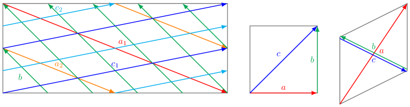
Figure S1: Brane configurations for the three two-tori (rectangles with opposite edges identified) in Model 22 where the third two-torus is tilted. Fermion mass hierarchies result from the intersections on the first two-torus.

Modular theta functions – Modular theta functions used in (44) and (73) are in general complicated to evaluate. However, for the special case without $B$-field, defining $J^{\prime}=-iJ=A$ and $\kappa^{\prime}=-i\kappa$ the $\vartheta$ function simplifies,

$$\vartheta\left[\begin{array}[]{c}\delta\\ \phi\end{array}\right](\kappa^{\prime})=\sum_{l\in\mathbbm{Z}}e^{-\pi\kappa^{\prime}(\delta+l)^{2}}e^{2\pi i(\delta+l)\phi}$$ (S3)

$$\stackrel{{\scriptstyle\rm{redefine}}}{{\xrightarrow{\hskip 19.91692pt}}} \vartheta\left[\begin{array}[]{c}\delta\\ \phi\end{array}\right](\kappa)=e^{-\pi\kappa\delta^{2}}e^{2\pi i\delta\phi}\vartheta_{3}(\pi(\phi+i\kappa\delta),e^{-\pi\kappa}),$$ (S6)

in terms of $\vartheta_{3}$, the Jacobi theta function of third kind. For $\kappa^{(1)}=64$ and $\epsilon^{(1)}_{u}=\epsilon^{(1)}_{d}=0$ and $\epsilon^{(1)}_{\nu}=\epsilon^{(1)}_{e}=\frac{1}{2}$ the couplings (44) where $T^{\nu}_{i}=T^{e}_{i}$ and $T^{u}_{i}=T^{d}_{i}$ are,

$$T^{\nu}_{0} =0 \quad T^{u}_{0} =1.$$

$$T^{\nu}_{1} =0 \quad T^{u}_{1} =0.24752$$

$$T^{\nu}_{2} =1.98503\times 10^{-10} \quad T^{u}_{2} =0.00375355$$

$$T^{\nu}_{3} =3.48734\times 10^{-6} \quad T^{u}_{3} =3.48734\times 10^{-6}$$

$$T^{\nu}_{4} =0.00375355 \quad T^{u}_{4} =1.98503\times 10^{-10}$$

$$T^{\nu}_{5} =0.24752 \quad T^{u}_{5} =0$$

$$T^{\nu}_{6} =1. \quad T^{u}_{6} =0$$

$$T^{\nu}_{7} =0.24752 \quad T^{u}_{7} =0$$

$$T^{\nu}_{8} =0.00375355 \quad T^{u}_{8} =1.98503\times 10^{-10}$$

$$T^{\nu}_{9} =3.48734\times 10^{-6} \quad T^{u}_{9} =3.48734\times 10^{-6}$$

$$T^{\nu}_{10} =1.98503\times 10^{-10} \quad T^{u}_{10} =0.00375355$$

$$T^{\nu}_{11} =0 \quad T^{u}_{11} =0.24752$$ (S7)

And the couplings (73) used in the simplified matrix (77) with only non-zero VEVs for $\epsilon^{(1)}_{4d}=1/2$ and $\epsilon^{(1)}_{4e}=0$ are,

$$\begin{array}[]{llll}F^{d}_{1}&=0.&\quad F^{e}_{1}&=0.604923\\ F^{d}_{17}&=0.&\quad F^{e}_{17}&=0.0108467\\ F^{d}_{19}&=0.&\quad F^{e}_{19}&=0.604923\\ \end{array}$$ (S8)

Figure S3 shows the logarithmic spectrum of all possible eigenvalues with $\kappa^{(2)}=64$ where the precise matching happens only at $\epsilon^{(2)}_{\nu}=1/2$.

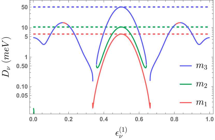
Figure S2: Log-plot of the spectrum of eigenvalues of the neutrino-masses as a function of brane-position parameter $\epsilon^{(2)}_{\nu}$ for $\kappa^{(2)}=64$. The dashed colored lines correspond to the mass-eigenvalues $\left(50.4,10.5,6.1\right)$ meV. The desired solution corresponds to the value $\epsilon^{(2)}_{\nu}=1/2$ where the respective curves simultaneously touch the dashed-lines.

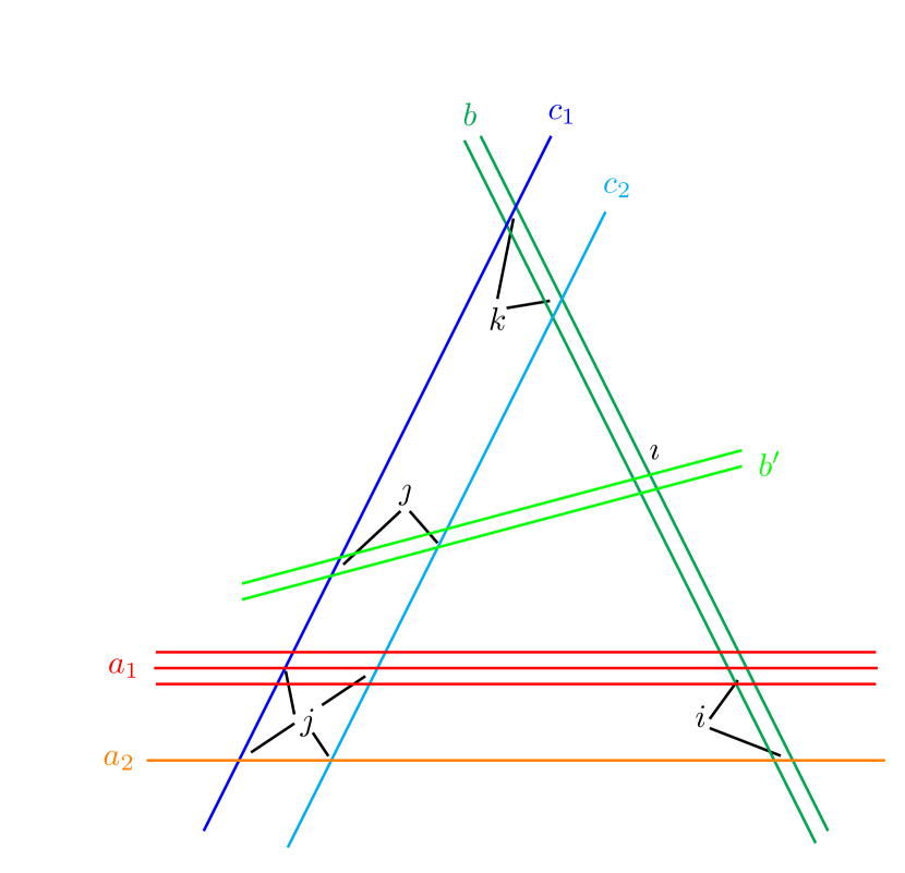
Figure S3: Yukawa couplings of the up-type quarks are from the areas by stack $a_{1}$, $b$, $c_{1}$, the down-type quarks by stack $a_{1}$, $b$, $c_{2}$, neutrinos by $a_{2}$, $b$, $c_{1}$ and the charged-leptons by $a_{2}$, $b$, $c_{2}$. The four-point function corrections to the Yukawa couplings of the charged-leptons by $a_{2}$, $b$, $b^{\prime}$, $c_{2}$.

Four-point corrections – We considered the 4-point interaction of $b$ brane with the triplet $a,b^{\prime},c$ by adding the following terms in the superpotential (Fermion Masses and Mixings in String Theory with Dirac Neutrinos),

$$\mathcal{W}_{4} \sim{1\over{M_{\rm S}}}\Big{(}Y^{\prime d}_{ijkl}Q_{i}D^{c}_{j}H^{\prime d}_{k}S^{L}_{l}+Y^{\prime e}_{ijkl}L_{i}E^{c}_{j}H^{\prime d}_{k}S^{L}_{l}\Big{)}.$$ (S9)

The notation of indices used in the (Fermion Masses and Mixings in String Theory with Dirac Neutrinos) can be discerned from the figure S3. We may calculate the areas of the triangles as we did in the trilinear Yukawa couplings,

$$A_{ijk} =\frac{1}{2}(2\pi)^{2}A_{\mathbf{T^{2}}}|I_{ab}I_{bc}I_{ca}|~{}\big{(}\frac{i}{I_{ab}}+\frac{j}{I_{ca}}+\frac{k}{I_{bc}}+\epsilon+l\big{)}^{2},$$

$$A_{\imath\jmath k} =\frac{1}{2}(2\pi)^{2}A_{\mathbf{T^{2}}}|I_{b^{\prime}b}I_{bc}I_{cb^{\prime}}|~{}\big{(}\frac{\imath}{I_{b^{\prime}b}}+\frac{\jmath}{I_{cb^{\prime}}}+\frac{k}{I_{bc}}+\varepsilon+\ell\big{)}^{2},$$ (S10)

where $i$, $j$, $k$ and $\imath$, $\jmath$, $k$ are using the same selection rules as (37). Thus, the classical contribution of the four-point functions is given by

$$Z_{4cl}=\sum_{l,\ell}e^{-\frac{1}{2\pi}|A_{ijk}-A_{\imath\jmath k}|}.$$ (S11)

The full classical four-point contribution to the mass matrix is given as column-wise splitted across three lines,

$$Z_{4cl}\!=\!\leavevmode\resizebox{411.93767pt}{}{ {\hbox{\begin{aligned} &\left( \begin{array}[]{c}F_{0} u_{1} w_{1}+F_{16} u_{13} w_{1}+F_{13} u_{12} w_{2}+F_{10} u_{11} w_{3}+F_{7} u_{10} w_{4}+F_{4} u_{9} w_{5}+F_{1} u_{8} w_{6}+F_{17} u_{20} w_{6}+F_{18} u_{7} w_{7}+F_{14} u_{19} w_{7}+F_{15} u_{6} w_{8}+F_{11} u_{18} w_{8}\\ F_{18} u_{12} w_{1}+F_{15} u_{11} w_{2}+F_{12} u_{10} w_{3}+F_{9} u_{9} w_{4}+F_{6} u_{8} w_{5}+F_{2} u_{20} w_{5}+F_{3} u_{7} w_{6}+F_{19} u_{19} w_{6}+F_{0} u_{6} w_{7}+F_{16} u_{18} w_{7}+F_{17} u_{5} w_{8}+F_{13} u_{17} w_{8}\\ F_{0} u_{11} w_{1}+F_{17} u_{10} w_{2}+F_{14} u_{9} w_{3}+F_{11} u_{8} w_{4}+F_{7} u_{20} w_{4}+F_{8} u_{7} w_{5}+F_{4} u_{19} w_{5}+F_{5} u_{6} w_{6}+F_{1} u_{18} w_{6}+F_{2} u_{5} w_{7}+F_{18} u_{17} w_{7}+F_{19} u_{4} w_{8}+F_{15} u_{16} w_{8}\\ \end{array}\right.\\ &\begin{array}[]{c}F_{18} u_{12} w_{1}+F_{15} u_{11} w_{2}+F_{12} u_{10} w_{3}+F_{9} u_{9} w_{4}+F_{6} u_{8} w_{5}+F_{2} u_{20} w_{5}+F_{3} u_{7} w_{6}+F_{19} u_{19} w_{6}+F_{0} u_{6} w_{7}+F_{16} u_{18} w_{7}+F_{17} u_{5} w_{8}+F_{13} u_{17} w_{8}\\ F_{0} u_{11} w_{1}+F_{17} u_{10} w_{2}+F_{14} u_{9} w_{3}+F_{11} u_{8} w_{4}+F_{7} u_{20} w_{4}+F_{8} u_{7} w_{5}+F_{4} u_{19} w_{5}+F_{5} u_{6} w_{6}+F_{1} u_{18} w_{6}+F_{2} u_{5} w_{7}+F_{18} u_{17} w_{7}+F_{19} u_{4} w_{8}+F_{15} u_{16} w_{8}\\ F_{2} u_{10} w_{1}+F_{19} u_{9} w_{2}+F_{16} u_{8} w_{3}+F_{12} u_{20} w_{3}+F_{13} u_{7} w_{4}+F_{9} u_{19} w_{4}+F_{10} u_{6} w_{5}+F_{6} u_{18} w_{5}+F_{7} u_{5} w_{6}+F_{3} u_{17} w_{6}+F_{4} u_{4} w_{7}+F_{0} u_{16} w_{7}+F_{1} u_{3} w_{8}+F_{17} u_{15} w_{8}\\ \end{array}\\ &\left.\begin{array}[]{c}F_{0} u_{11} w_{1}+F_{17} u_{10} w_{2}+F_{14} u_{9} w_{3}+F_{11} u_{8} w_{4}+F_{7} u_{20} w_{4}+F_{8} u_{7} w_{5}+F_{4} u_{19} w_{5}+F_{5} u_{6} w_{6}+F_{1} u_{18} w_{6}+F_{2} u_{5} w_{7}+F_{18} u_{17} w_{7}+F_{19} u_{4} w_{8}+F_{15} u_{16} w_{8}\\ F_{2} u_{10} w_{1}+F_{19} u_{9} w_{2}+F_{16} u_{8} w_{3}+F_{12} u_{20} w_{3}+F_{13} u_{7} w_{4}+F_{9} u_{19} w_{4}+F_{10} u_{6} w_{5}+F_{6} u_{18} w_{5}+F_{7} u_{5} w_{6}+F_{3} u_{17} w_{6}+F_{4} u_{4} w_{7}+F_{0} u_{16} w_{7}+F_{1} u_{3} w_{8}+F_{17} u_{15} w_{8}\\ F_{4} u_{9} w_{1}+F_{1} u_{8} w_{2}+F_{17} u_{20} w_{2}+F_{18} u_{7} w_{3}+F_{14} u_{19} w_{3}+F_{15} u_{6} w_{4}+F_{11} u_{18} w_{4}+F_{12} u_{5} w_{5}+F_{8} u_{17} w_{5}+F_{9} u_{4} w_{6}+F_{5} u_{16} w_{6}+F_{6} u_{3} w_{7}+F_{2} u_{15} w_{7}+F_{3} u_{2} w_{8}+F_{19} u_{14} w_{8}\\ \end{array}\right). \end{aligned}}}}$$ (S12)

References

Supplemental Material to