Perm: A Parametric Representation for Multi-Style 3D Hair Modeling

Abstract.

We present Perm, a learned parametric model of human 3D hair designed to facilitate various hair-related applications. Unlike previous work that jointly models the global hair shape and local strand details, we propose to disentangle them using a PCA-based strand representation in the frequency domain, thereby allowing more precise editing and output control. Specifically, we leverage our strand representation to fit and decompose hair geometry textures into low- to high-frequency hair structures. These decomposed textures are later parameterized with different generative models, emulating common stages in the hair modeling process. We conduct extensive experiments to validate the architecture design of Perm, and finally deploy the trained model as a generic prior to solve task-agnostic problems, further showcasing its flexibility and superiority in tasks such as 3D hair parameterization, hairstyle interpolation, single-view hair reconstruction, and hair-conditioned image generation. Our code and data will be available at: https://github.com/c-he/perm.

Figure 1. Perm is a learned parametric model of 3D human hair that is designed with disentangled parameters $\vec{\theta}$ and $\vec{\beta}$ to respectively control the global hair shape (represented as guide strands) and local strand details (e.g., curliness).

1. Introduction

				“wavy and short hair, white sweater”
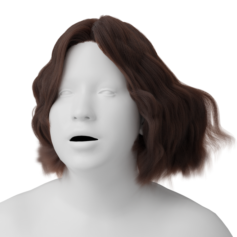
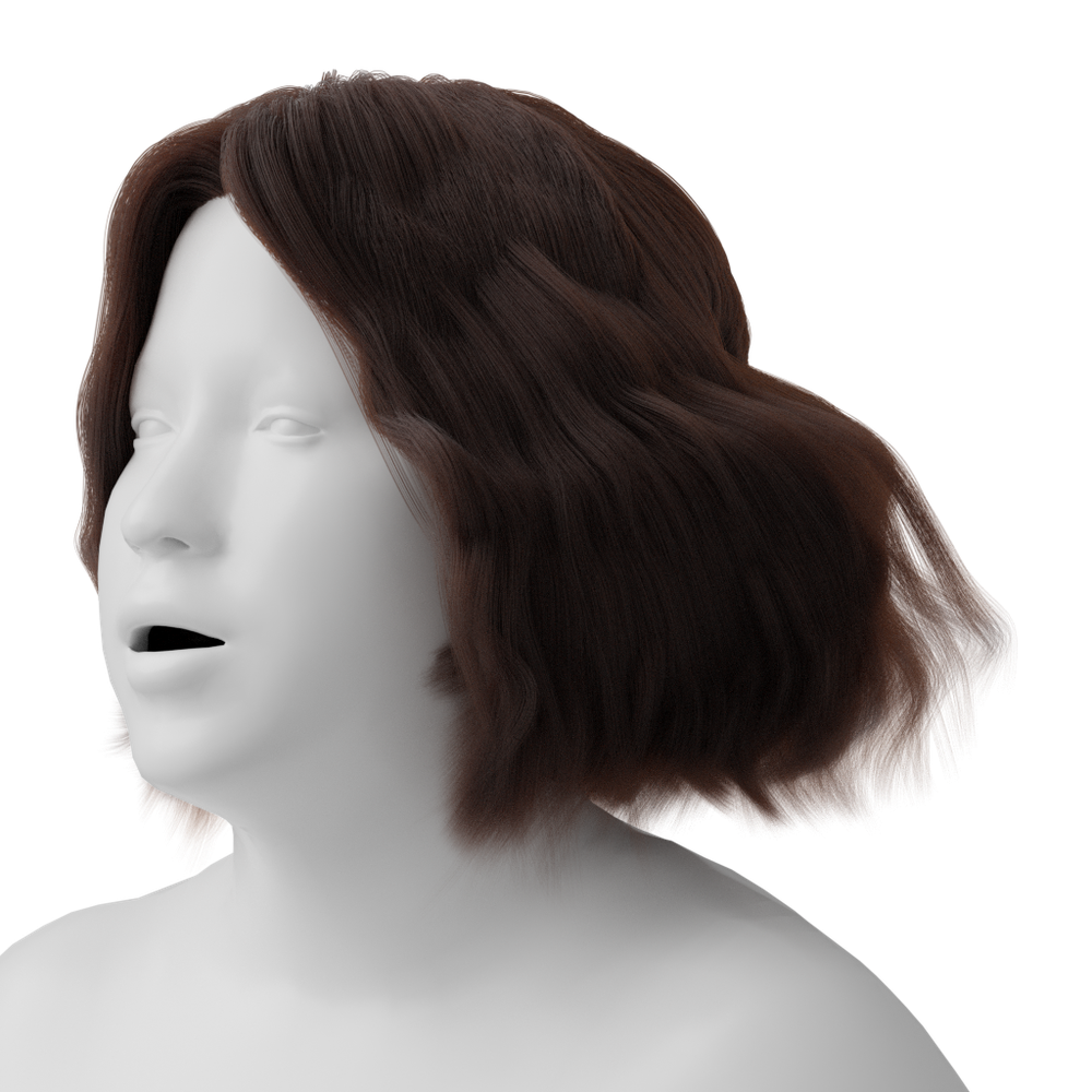
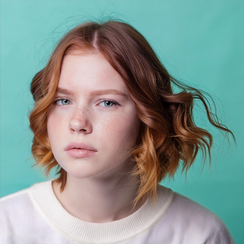
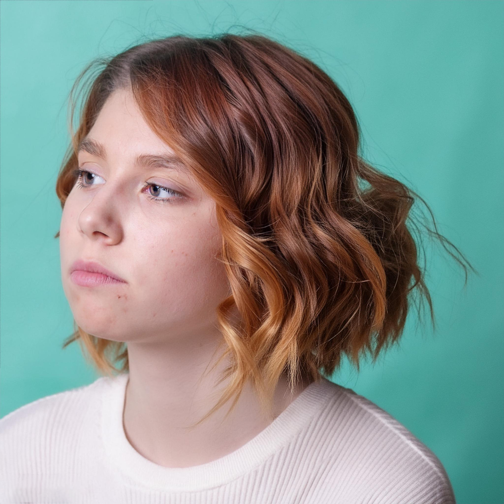
Input Image	Single-view Recon.	Perm Parameter Editing		Hair-conditioned Image Generation

Figure 2. An application demo of Perm, where we first fit Perm parameters to reconstruct 3D hair from the input image, then edit the parameters to change its style from straight to wavy, and finally use the edited hairstyle and certain viewing direction as a condition for image generation with Adobe Firefly [Adobe, 2024].

Hair, as a crucial component in the realm of digital humans, has been studied for decades in computer graphics. With the recent availability of high-quality 3D hair data [Hu et al., 2015; Shen et al., 2023], numerous methods have emerged in the field of hair modeling, demonstrating their effectiveness in applications such as hair manipulation [Chai et al., 2013; Weng et al., 2013], hair dynamics modeling [Yang et al., 2019; Wang et al., 2023b], novel hairstyle synthesis [Zhou et al., 2023; Sklyarova et al., 2023b], and 3D hair reconstruction either from images [Wu et al., 2022; Zheng et al., 2023; Takimoto et al., 2024; Kuang et al., 2022] or monocular videos [Wu et al., 2024; Luo et al., 2024; Sklyarova et al., 2023a]. Despite their achievements, these methods often overlook the inherent biscale nature of hair, where hairstyles with similar global shapes may exhibit variations in local details. For instance, blowout hairstyles with a similar shape can have variations ranging from a sleek and smooth straight look to more modern styles such as beach waves or bouncy curls, depending on the blow-drying techniques employed. Neglecting these biscale variations limits the generation and editing capability, hindering applications such as changing a hairstyle from straight to curly while maintaining a similar haircut. Moreover, most of the models proposed in existing methods are task-specific, lacking the generalization capability to different down-stream tasks. In contrast, the field of human body modeling has well-accepted parametric models like SMPL [Loper et al., 2015] and MANO [Romero et al., 2017], which designed disentangled coefficients for pose and shape and are widely applied as a generic prior in deep learning applications such as human reconstruction and animation. To address this gap, we propose Perm, a parametric model of 3D human hair that can serve as an effective prior for various hair-related applications.

Perm is formulated as $\mathcal{M}(\vec{\theta},\vec{\beta},\mathcal{R})$, where the output hair is conditioned on the guide strand parameter $\vec{\theta}$ for its global shape, the hair styling parameter $\vec{\beta}$ for its local details, and a pre-defined root set $\mathcal{R}$ for the hair density. To independently control the global shape and local details, we propose a strand representation based on principal component analysis (PCA) in the frequency domain, which fits the nearly periodic behavior of hair strands. The learned principal components form an explainable space for hair decomposition, where the initial components capture low-frequency information, such as rough shape and large deformation, and the subsequent components encode high-frequency details like curliness. Based on this strand representation, we fit geometry textures for each hairstyle and decompose them into guide textures for guide strands and residual textures for local strand details, facilitating precise editing and output control. With these decomposed texture maps, we design different generative models to emulate common modeling stages in existing hair modeling software like Maya XGen [Autodesk, 2024]. Specifically, we train a StyleGAN2 [Karras et al., 2020] for guide textures, serving as an automated guide strand authoring system conditioned on parameters. We train a Variational Autoencoder (VAE) [Kingma and Welling, 2013] for residual textures, replacing those procedures with learned but not manually designed parameters. Finally, we introduce a U-Net [Ronneberger et al., 2015] super resolution module to upsample guide textures, replicating the guide interpolation stage.

After training Perm, we demonstrate its capability across multiple applications, including 3D hair parameterization, hairstyle interpolation, and single-view hair reconstruction. Despite not being trained specifically for any of these tasks, Perm achieves performance equivalent or superior to state-of-the-art task-specific alternatives in our experiments. Moreover, we introduce a novel application of using Perm-generated hair for conditional image generation. A demo of these applications is provided in Fig. 2.

Our code and data will be publicly available after review process.

2. Related Work

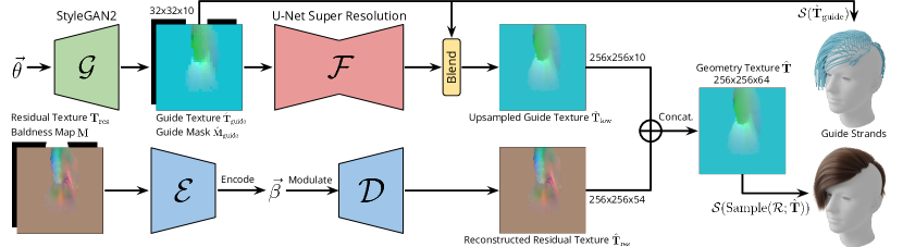
Figure 3. Overview of Perm, where a guide strand function $\mathcal{G}(\vec{\theta})$ takes the parameter $\vec{\theta}$ to synthesize the guide texture $\hat{\mathbf{T}}_{\text{guide}}$ and guide mask $\hat{\mathbf{M}}_{\text{guide}}$. They are then super-resolved with the function $\mathcal{F}(\cdot)$ to obtain the upsampled texture $\hat{\mathbf{T}}_{\text{low}}$. For the high-frequency part, a hair styling function $\mathcal{D}(\vec{\beta})$ maps the parameter $\vec{\beta}$ to the residual texture $\hat{\mathbf{T}}_{\text{res}}$. These two textures are concatenated to from the geometry texture $\hat{\mathbf{T}}$, which can finally be sampled and decoded with the function $\mathcal{S}(\cdot)$ to obtain the strand geometry.

The unstructured nature of hair makes its modeling a long and tedious process. For decades people have been studying advanced ways to model hair geometries. Here we review this literature.

Geometric Hair Modeling

Techniques for geometric hair modeling typically involve explicit descriptions of hair structure. Observing the similarity among neighboring hair strands, early approaches utilize representations such as wisps [Watanabe and Suenaga, 1992], bundles of cylinders [Chen et al., 1999], or coarse polygonal meshes [Yuksel et al., 2009]. Similar strip representations have also been employed in reconstructing hair from single [Chai et al., 2016a] or multiple images [Luo et al., 2013], as well as in interactive hair modeling and immersive control [Xing et al., 2019]. However, as these low-resolution geometric-based models often lack fine-grained details, subsequent works shifted their focus to model each strand as a sequence of connected 3D points, resulting in methods utilizing 3D vector fields  [Fu et al., 2007; Chai et al., 2012, 2013; Zhang et al., 2017; Shen et al., 2020]. Furthermore, hair can be modeled with multi-resolution [Kim and Neumann, 2002] or multi-scale geometric representations [Wang et al., 2009; Weng et al., 2013]. Similar to these approaches, we decompose hair models into multi-scale features and use a scalp texture to record strand features. However, we aim at generating a variety of hairstyles, rather than variations of a single style.

Volumetric Hair Modeling

To reconstruct 3D hair from real-world observations, several pioneering methods have been proposed with specialized hardware devices [Nam et al., 2019; Shen et al., 2023; Hu et al., 2014; Jakob et al., 2009; Herrera et al., 2012; Xu et al., 2014; Paris et al., 2004; Grabli et al., 2002; Wei et al., 2005], which are often expensive and unsuitable for wide application. Alternatively, some methods use single or multiple captured images to retrieve hair models from a pre-stored database [Hu et al., 2014, 2015; Zhang et al., 2018; Liang et al., 2018], offloading the burden of hardware setup to the computational cost of database search and result refinement. To mitigate the high cost of database retrieval, deep learning techniques have been proposed to non-linearly parameterize the large variations of 3D hair datasets [Saito et al., 2018; Zhang and Zheng, 2019]. Existing approaches often rely on volumetric fields as an efficient spatial-aware intermediate representation to encode hair, spanning from sketch-based hair modeling [Shen et al., 2020], video-based dynamic hair modeling [Yang et al., 2019], to 3D hair reconstruction from either images [Wu et al., 2022; Zheng et al., 2023; Takimoto et al., 2024; Kuang et al., 2022] or monocular videos [Wu et al., 2024; Luo et al., 2024; Sklyarova et al., 2023a]. However, entangled volumetric fields are not well-suited for representing curly and kinky hair. To better capture hair, Wang et al. [2022; 2023a] learn fine-grained details of hair implicitly encoded in multiple neural volumetric primitives, which are attached to pre-obtained sparse guide strands. They also developed a neural volumetric renderer to model dynamic hair [Wang et al., 2023b].

Hair Geometry Textures

Organizing strand features within the scalp texture [Wang et al., 2009] provides a 2D representation of hair that can be learned using 2D convolution networks [Zhou et al., 2018; Rosu et al., 2022], commonly referred to as geometry textures [Sklyarova et al., 2023a]. This texture-based representation also facilitates the application of diffusion models [Ho et al., 2020] for hair modeling. For instance, Neural Haircut [Sklyarova et al., 2023a] leverages a pre-trained diffusion prior to generate hair geometry textures, which serve as cues for reconstructing high-fidelity hairstyles from smartphone video captures. Similarly, HAAR [Sklyarova et al., 2023b] introduces a text-conditioned diffusion model for 3D strand-based hairstyle generation, utilizing geometry textures as input to encode latent hairstyle representations. While these diffusion-based methods produce impressive results, they typically involve a heavy denoising process and lack a compact latent space for hair reconstruction and editing. The work most related to our approach is GroomGen [Zhou et al., 2023], which constructed hierarchical hair latent spaces represented in the scalp texture space. Unlike previous work, we do not use a single hair texture map to directly record strand latent features. Instead, we represent hair strands with multiple frequency components to generate hierarchical hair geometry textures from low- to high-frequency. As a result, our work offers independent control over the global hair shape and local strand details.

Parametric Modeling

In human digitalization, Blanz et al. [1999] first proposed a 3D statistical morphable face model using PCA to parameterize the face modeling space. After that, subsequent works have leveraged PCA-based parametric modeling for 3D facial expressions [Cao et al., 2014] and whole body reconstruction [Allen et al., 2003]. SMPL [Loper et al., 2015] extended this PCA-based idea to model a whole range of body shapes and poses, with its follow-up work SMPL-X [Pavlakos et al., 2019] capturing the body, hand, and face together by integrating SMPL with the FLAME [Li et al., 2017] head model and the MANO [Romero et al., 2017] hand model. Similar ideas can be applied to model animals [Zuffi et al., 2017], infants [Hesse et al., 2018], and cartoon characters [Luo et al., 2023]. For hair modeling, guide strands are commonly used as a reduced parameterization. Chai et al. [2014] presented a reduced hair model by parameterizing the dynamic hair space with selected guide strands. They extended this work with an adaptive skinning method for interactive hair-solid simulation [Chai et al., 2016b]. Following a similar idea, Lyu et al. [2020] employ a neural interpolator to generate adaptive dynamic weights on-the-fly to interpolate guide strands. However, due to the absence of a known principal basis for hair geometries that generalizes to all hairstyles, there is no parametric model for hair styling. To tackle this, we explore the frequency domain of hair strands and develop a hybrid hierarchical parametric hair representation, incorporating both linear and non-linear parameterizations across different hairstyles.

3. Model Formulation

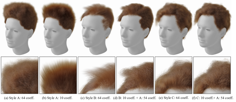
Figure 4. With our PCA-based strand representation, we can smooth a hairstyle by truncating its strand PCA coefficient from $64$ (a) to $10$ (b). By blending the low-rank and high-rank PCA coefficients from different hairstyles, we can create diverse composite hairstyles (d and f). Please zoom-in for details.

The architecture of Perm is illustrated in Fig. 3, which imitates the current hair modeling pipeline in industrial software like XGen. Starting from a PCA-based strand representation in the frequency domain (Sec. 3.1), we design a function, $\mathcal{S}(\vec{\gamma}):\mathbb{R}^{|\vec{\gamma}|}\mapsto\mathbb{R}^{L\times 3}$, that maps the strand PCA coefficients $\vec{\gamma}$ back to 3D polylines with $L$ points (where $L$ is set to $100$ in our experiments). These PCA coefficients are then employed to fit 2D geometry textures to represent the 3D hair, which are further decomposed and parameterized with a guide strand function $\mathcal{G}(\vec{\theta})$, a super resolution function $\mathcal{F}(\cdot)$, and a hair styling function $\mathcal{D}(\vec{\beta})$ with controlling parameters $\vec{\theta}$ and $\vec{\beta}$ (Sec. 3.2). The resulting Perm model can thus be expressed as:

(1) $$\mathcal{M}(\vec{\theta},\vec{\beta},\mathcal{R};\Phi)=\mathcal{S}\Big{(}\text{Sample}\big{(}\mathcal{R};\mathcal{F}(\mathcal{G}(\vec{\theta}))\oplus\mathcal{D}(\vec{\beta})\big{)}\Big{)},$$

where $\text{Sample}(\cdot)$ denotes nearest neighbor interpolation used to sample the synthesized texture with 2D root coordinates in the pre-defined root set $\mathcal{R}$, $\oplus$ represents the concatenation operation along the feature channels, and $\Phi$ specifies the full set of trainable parameters of Perm. Once trained, parameters in $\Phi$ are held fixed, and novel 3D hairstyles are synthesized by varying $\vec{\theta}$ and $\vec{\beta}$ respectively, while the hair density can be adjusted by manipulating the number of roots in $\mathcal{R}$. The dimension of parameters $\vec{\theta}$ and $\vec{\beta}$ are both set to $512$ in our model ($|\vec{\theta}|=|\vec{\beta}|=512$). In the following, we delve into the details of each term in our model.

3.1. Strand Parameterization

Inspired by the nearly periodic behavior of hair strands, we define a low-dimensional parameter space based on PCA in the frequency domain. Formally, given hair strands represented with a fixed number of points $\mathbf{S}=\{\mathbf{p}_{1},\mathbf{p}_{2},\dots,\mathbf{p}_{L}\}\in\mathbb{R}^{L\times 3}$, we parameterize them with a linear function $\mathcal{S}$ in the frequency domain:

(2) $$\mathcal{S}(\vec{\gamma};\mathbf{X})=\text{iDFT}(\bar{\mathbf{S}}+\vec{\gamma}^{\top}\mathbf{X})=\text{iDFT}(\bar{\mathbf{S}}+\sum_{n=1}^{|\vec{\gamma}|}\vec{\gamma}_{n}\mathbf{X}_{n}),$$

where $\bar{\mathbf{S}}=[\bar{\mathbf{S}}_{\text{real}},\bar{\mathbf{S}}_{\text{imag}}]\in\mathbb{R}^{k\times 3\times 2}$ denotes the mean phase vector of strands, with $k=\lfloor L/2\rfloor+1$ representing the number of frequency bands. $\mathbf{X}=[\mathbf{X}_{1},\mathbf{X}_{2},\dots,\mathbf{X}_{|\vec{\gamma}|}]^{\top}\in\mathbb{R}^{|\vec{\gamma}|\times 6k}$ forms a matrix of orthonormal principal components that capture phase variations in different strands, and $\text{iDFT}(\cdot)$ represents the inverse Discrete Fourier Transform that maps strands back from the frequency domain to the spatial domain. Therefore, a 3D strand $\mathbf{S}$ is represented as a vector of linear coefficients $\vec{\gamma}=[\gamma_{1},\dots,\gamma_{|\vec{\gamma}|}]^{\top}$. In other sections, we will omit $\mathbf{X}$ in Eq. 2 for brevity.

To obtain quantities in Eq. 2, we first apply the Discrete Fourier Transform (DFT) along the $x$, $y$, $z$ axes to all strands in our collected hair models, and then compute the mean phase vector $\bar{\mathbf{S}}$ and solve the principal components $\mathbf{X}$ by performing PCA on the computed Fourier bases, which is similar to the prevalent PCA-based modeling methods in digital humans [Blanz and Vetter, 1999; Loper et al., 2015; Li et al., 2017]. We set the number of PCA coefficients $|\vec{\gamma}|=64$, which explained almost $100\%$ of the variance in the training set.

Our strand representation differs from previous work [Rosu et al., 2022; Sklyarova et al., 2023a; Zhou et al., 2023] that uses a VAE to learn the strand latent space. Throughout our experiments, this simple yet effective formulation attained comparable or superior performance compared to those carefully designed VAEs. It also significantly reduces training time and GPU memory consumption due to its analytical computation. Additionally, our frequency-based formulation offers an improved preservation of strand curvatures, which aligns with the findings in GroomGen [Zhou et al., 2023].

Our PCA-based representation also facilitates a meaningful decomposition of strand geometry by forming an explainable parameter space. Our analysis reveals that the first $10$ PCA coefficients are enough to effectively capture the rough shape of each strand, and the remaining $54$ coefficients encode high-frequency details, such as strand curliness. Leveraging this intuitive decomposition, we can effortlessly smooth a given hairstyle by truncating its strand PCA coefficients (Fig. 4a, b), or create diverse styles by blending the low-rank and high-rank portions of PCA coefficients from different hairstyles (Fig. 4c-f).

3.2. Hairstyle Parameterization

With our proposed strand parameterization, we define a 2D parameterization of hairstyles on the scalp surface as a regular $uv$ texture map, where each texel stores the corresponding strand PCA coefficients $\vec{\gamma}$. These textures are referred to as hair geometry textures, denoted as $\mathbf{T}\in\mathbb{R}^{256\times 256\times 64}$. Similar to GroomGen [Zhou et al., 2023], we separately model the baldness area as a baldness map $\mathbf{M}\in\mathbb{R}^{256\times 256}$. Both $\mathbf{T}$ and $\mathbf{M}$ are downsampled to $32\times 32$ to represent guide strands (denoted as the guide texture $\mathbf{T}_{\text{guide}}$ and guide mask $\mathbf{M}_{\text{guide}}$), where only the low-rank PCA coefficients ($|\vec{\gamma}_{\text{guide}}|=10$) are kept in $\mathbf{T}_{\text{guide}}$, akin to those guide strands created by real users in professional hair modeling software. As not all texels will be decoded to meaningful strands, $\mathbf{T}_{\text{guide}}$ typically accommodates around $400$ strands, as visualized in Fig. 1. More technical details are given in Supplemental A.1. Motivated by deep learning-based methods [Zhou et al., 2023; Saito et al., 2018], we further decompose and parameterize our hair geometry textures with separate neural networks to align with existing hair modeling stages, namely guide strand synthesis, guide interpolation, and hair styling.

3.2.1. Guide Strand Synthesis

Formally, for guide strands, we train a neural network to approximate the function, $\mathcal{G}(\vec{\theta};\phi_{1})$: $\mathbb{R}^{|\vec{\theta}|}\mapsto\mathbb{R}^{32\times 32\times(10+1)}$, which synthesizes $\mathbf{T}_{\text{guide}}$ and $\mathbf{M}_{\text{guide}}$ from the guide strand parameter $\vec{\theta}$, where $\phi_{1}$ denotes the trainable network parameters. In our formulation, we choose StyleGAN2 [Karras et al., 2020] as the backbone of our model, which has been proved to be a powerful generator in both 2D images and 3D feature tri-planes [Chan et al., 2022]. It also ensures our guide strand parameter to follow the normal distribution $\vec{\theta}\sim\mathcal{N}(\bm{0},\bm{1})$, making it easy to sample. Moreover, the intermediate $\mathcal{W}$ and $\mathcal{W}+$ spaces introduced in StyleGAN allow for more faithful latent embedding [Abdal et al., 2019], which in our case facilitates hair reconstruction either from 3D strands or 2D orientation images. Since our generator synthesizes both the guide texture $\mathbf{T}_{\text{guide}}$ and guide mask $\mathbf{M}_{\text{guide}}$, we use a similar dual discrimination method as EG3D [Chan et al., 2022], where we concatenate these two images and feed them into the discriminator. This operation ensures consistency between the generated texture and mask, which helps the generator to place zero-length strands in bald areas. Our training objective is identical to StyleGAN2, which consists of a non-saturating GAN loss [Goodfellow et al., 2014] with $R_{1}$ regularization [Mescheder et al., 2018] on both the texture and mask, where the regularization strengths are set to $5$ and $1$, respectively.

3.2.2. Guide Interpolation

Since guide strands only serve as a sparse representation of the full hair, an upsampling process is necessary to obtain the final hair strands. However, as illustrated in GroomGen, this process entails a one-to-many mapping [Zhou et al., 2023], wherein the same guide strands can be upsampled to yield diverse hairstyles with varying strand randomness and curliness. Achieving this property proves challenging, necessitating an orthogonal decomposition of the global hair shape and local strand details. Previous methods thus either downgraded to a deterministic one-to-one mapping [Sklyarova et al., 2023b] or resorted to a manual post-processing step [Zhou et al., 2023]. To address this challenge, we further decompose our hair geometry texture $\mathbf{T}$ into $\mathbf{T}_{\text{low}}\in\mathbb{R}^{256\times 256\times 10}$ and $\mathbf{T}_{\text{res}}\in\mathbb{R}^{256\times 256\times 54}$ by splitting along the feature channels. Given the explainability of our strand PCA coefficients, we discern that $\mathbf{T}_{\text{low}}$ encapsulates the global hair shape, while $\mathbf{T}_{\text{res}}$ embodies the local strand details, denoted as the residual texture. Leveraging this decomposition, we employ different neural networks to parameterize them, simulating the automated processes of guide interpolation and hair styling. In this section, we will introduce the guide interpolation process, which generates $\mathbf{T}_{\text{low}}$ from the texture $\mathbf{T}_{\text{guide}}$ and mask $\mathbf{M}_{\text{guide}}$, and the subsequent stage will be elaborated in Sec. 3.2.3.

With our texture-based representation for 3D hair, guide interpolation becomes an image super resolution problem, which can be defined as the function, $\mathcal{F}(\mathbf{T}_{\text{guide}},\mathbf{M}_{\text{guide}};\phi_{2}):\mathbb{R}^{32\times 32\times 11}\mapsto\mathbb{R}^{256\times 256\times 10}$, with trainable network parameters $\phi_{2}$. Note that this function operates as a deterministic mapping without parameter control, which aligns with both previous deep learning-based methods [Zhou et al., 2023; Sklyarova et al., 2023b] and the adaptive interpolation algorithm used in current hair modeling software.

To approximate $\mathcal{F}(\cdot)$, we train a U-Net [Ronneberger et al., 2015] on the bilinearly upsampled textures, which translates them to $14$-channel weight maps, where the first $4$ channels represent the weight vector $\vec{\omega}$ for the $4$ neighboring guide strands, and the last $10$ channels represent a residual vector $\vec{\delta}$ to correct the blended coefficients. Therefore, the final coefficient $\vec{\gamma}_{\text{low}}$ can be calculated as:

(3) $$\vec{\gamma}_{\text{low}}=\vec{\omega}^{\top}\bm{\gamma}_{\text{guide}}+\vec{\delta}=\sum_{n=1}^{4}\omega_{n}\vec{\gamma}_{\text{guide}}^{n}+\vec{\delta}.$$

Our experiments demonstrate that this weight-based blending output allows the network to converge to a sharper result compared to predicting coefficients directly.

We train the U-Net in a supervised manner, where we employ both an $L_{1}$ loss for the blended texture $\hat{\mathbf{T}}_{\text{low}}$ and a geometric loss $\mathcal{L}_{\text{geo}}$ for the decoded strand geometry. Specifically, the geometric loss $\mathcal{L}_{\text{geo}}$ encompasses an $L_{1}$ loss for the point position $\hat{\mathbf{p}}_{n}$, a cosine distance for the orientation $\hat{\mathbf{d}}_{n}=\hat{\mathbf{p}}_{n+1}-\hat{\mathbf{p}}_{n}$[Rosu et al., 2022], and an $L_{1}$ loss for the curvature, represented as the $L_{2}$ norm of binormal vector $\hat{\mathbf{b}}_{n}=\|\hat{\mathbf{d}}_{n}\times\hat{\mathbf{d}}_{n+1}\|_{2}$[Sklyarova et al., 2023a]:

(4) $$\mathcal{L}_{\text{geo}}=\sum_{n=1}^{L}\|\hat{\mathbf{p}}_{n}-\mathbf{p}_{n}\|_{1}+(1-\hat{\mathbf{d}}_{n}\cdot\mathbf{d}_{n})+\|\hat{\mathbf{b}}_{n}-\mathbf{b}_{n}\|_{1}.$$

A regularization term is included as well to constrain the residual vector $\vec{\delta}$ towards $0$. The overall loss function, denoted as $\mathcal{L}_{\text{superres}}$, then can be expressed as:

(5) $$\mathcal{L}_{\text{superres}}=\lambda_{\text{tex}}\|\hat{\mathbf{T}}_{\text{low}}-\mathbf{T}_{\text{low}}\|_{1}+\lambda_{\text{geo}}\mathcal{L}_{\text{geo}}+\lambda_{\text{reg}}\|\vec{\delta}\|_{2}^{2},$$

where the weighting factors $\lambda_{\text{tex}}$, $\lambda_{\text{geo}}$ and $\lambda_{\text{reg}}$ are set to $1$, $1$ and $0.1$, respectively.

3.2.3. Hair Styling

To capture local details such as high-frequency curliness and randomness, artists employ various procedures to synthesize them from manually designed parameters. In our formulation, we approximate this artistic process by training a neural network. This network can be defined as the function, $\mathcal{D}(\vec{\beta};\phi_{3}):\mathbb{R}^{|\vec{\beta}|}\mapsto\mathbb{R}^{256\times 256\times 54}$, where we learn to synthesize the residual texture $\mathbf{T}_{\text{res}}$ from the hair styling parameter $\vec{\beta}$, and $\phi_{3}$ represents the trainable network parameters.

Although StyleGAN2 performs well in generating textures for guide strands, we found it struggles with residual textures, as they contain more data than high-resolution RGB images. Therefore, we opted for VAE [Kingma and Welling, 2013] as the backbone, where the encoder adopts an architecture similar to pSp [Richardson et al., 2021], and the decoder takes the same architecture as StyleGAN2 generator. Essentially, the encoder $\mathcal{E}$ projects the residual texture $\mathbf{T}_{\text{res}}$ and baldness map $\mathbf{M}$ into the latent space, where the latent vectors will then be used to modulate the decoder to reconstruct the input. A similar loss function as Eq. 5 is defined as the training objective for the VAE, which can be expressed as:

(6) $$\mathcal{L}_{\text{res}}=\lambda_{\text{tex}}(\|\hat{\mathbf{T}}_{\text{res}}-\mathbf{T}_{\text{res}}\|_{1}+\|\hat{\mathbf{M}}-\mathbf{M}\|_{1})+\lambda_{\text{geo}}\mathcal{L}_{\text{geo}}+\lambda_{\text{KL}}\mathcal{L}_{\text{KL}},$$

where the reconstruction terms are computed on the residual texture, baldness map, and decoded strand geometry. The weighting factors $\lambda_{\text{tex}}$, $\lambda_{\text{geo}}$, and $\lambda_{\text{KL}}$ are set to $10$, $1$, and $1e^{-4}$, respectively.

After synthesizing residual textures, they can be concatenated with the upsampled guide textures, thereby composing the final hair geometry textures. These textures can then be sampled and decoded to produce the final strand geometry.

4. Experiments and Results

We train Perm on USC-HairSalon [Hu et al., 2015], a dataset comprising $343$ 3D hair models collected from online game communities. After augmentation, our training set contains a total of $21,054$ data samples. For evaluation, we compiled a dataset consisting of $17$ publicly available and $100$ artist-groomed hair models. Details are provided in Supplemental B.1.

4.1. Evaluation and Comparison

4.1.1. Strand Representation

We evaluate our PCA-based strand representation by comparing it to alternative deep learning-based methods [Zhou et al., 2023; Rosu et al., 2022; Sklyarova et al., 2023a] and a simpler PCA-based formulation without DFT. To quantitatively assess their reconstruction capabilities, we present the mean position error (pos. err.), computed as the average Euclidean distance between corresponding points on the reconstructed strands and the ground truth. Additionally, we report the mean curvature error (cur. err.), defined as the $L_{1}$ norm between the curvatures of reconstructed and ground truth strands. Please refer to Supplemental B.3 for details of the metrics.

Table 1. Reconstruction errors reported on different strand representations.

	Pos. VAE	Freq. VAE	Pos. PCA	Freq. PCA
# params.	$15.67$M	$16.51$M	$19.31$K	$19.50$K
pos. err.	$0.075$	$0.726$	$\bm{0.004}$	$\bm{0.004}$
cur. err.	$0.860$	$\bm{0.304}$	$1.229$	$0.569$

Quantitative results are reported in Table 1, where all configurations compress strands to $64$-dimensional vectors. Our PCA-based representations demonstrate a remarkably small position error, achieving this with a significantly reduced number of parameters compared to strand VAEs trained either in the spatial [Rosu et al., 2022; Sklyarova et al., 2023a] or frequency domain [Zhou et al., 2023]. While performing PCA on strand positions results in a relatively high curvature error, performing PCA in the frequency domain effectively mitigates this issue, demonstrating superior preservation of strand curvatures. Note that, although the strand VAE trained in the frequency domain attains the lowest curvature error, it does not preserve the overall shape, thus leading to a high position error (see Fig. 5).

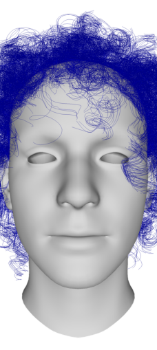
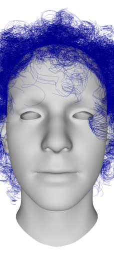
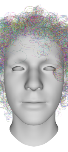
	Pos. VAE	Freq. VAE	Pos. PCA	Freq. PCA	Ground Truth

Figure 5. Comparison of our PCA-based strand representation (Freq. PCA) with other VAE-based representations (Pos. VAE [Rosu et al., 2022; Sklyarova et al., 2023a], Freq. VAE [Zhou et al., 2023]) and a simpler PCA-based formulation in the spatial domain (Pos. PCA). Reconstructed strands are color-coded by their position error. More results are available in Fig. 3 of our supplemental.

4.1.2. Guide Strand Synthesis

Table 2. Reconstruction errors reported on different model representations.

	Guide Strands		Full Hair
	PCA	StyleGAN2 (Ours)	GroomGen	Ours
pos. err.	$3.734$	$\bm{0.491}$	$2.584$	$\bm{0.805}$
cur. err.	$4.212$	$\bm{0.281}$	$3.442$	$\bm{0.179}$

To assess the performance of StyleGAN2 in guide strand synthesis, we create a PCA-based representation for guide textures with a similar formulation as our strand parameterization, and set the subspace dimension to $512$ to align with Perm’s setup. We then embed guide textures in the testing set into the PCA subspace or the latent space learned by StyleGAN2, followed by a decoding step to reconstruct them. Strands are further decoded from the reconstructed textures to evaluate quantitative errors, which are reported in Table 2 ($1$st and $2$nd columns). It is evident that results from StyleGAN2 exhibit both smaller position and curvature errors, indicating that StyleGAN2 learns a more expressive latent space than PCA. Fig. 6 displays examples of reconstructed guide strands, illustrating that StyleGAN2 more faithfully preserves the structure of the ground truth. Reasons for the failure of PCA are straightforward: USC-HairSalon contains a vast number of strands, specifically $3,150,559$, for us to learn the PCA subspace, with a compression rate of approximately $78.7\%$. However, for guide textures, we can only create $21,054$ samples after data augmentation, which is merely around $0.6\%$ of the total number of available strands. Moreover, the compression rate increases to $95\%$. These two factors lead to the poor performance of PCA in this case.

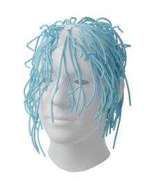
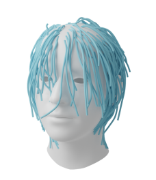
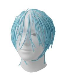
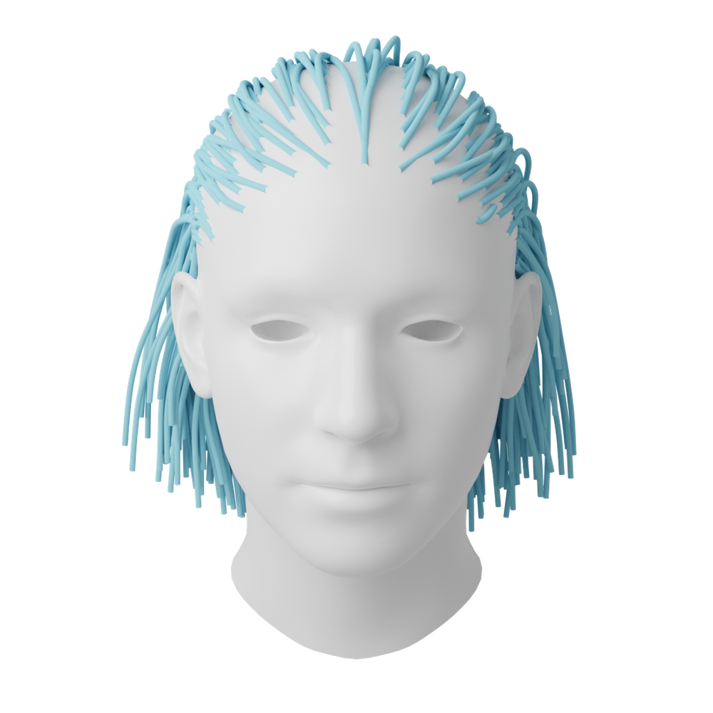
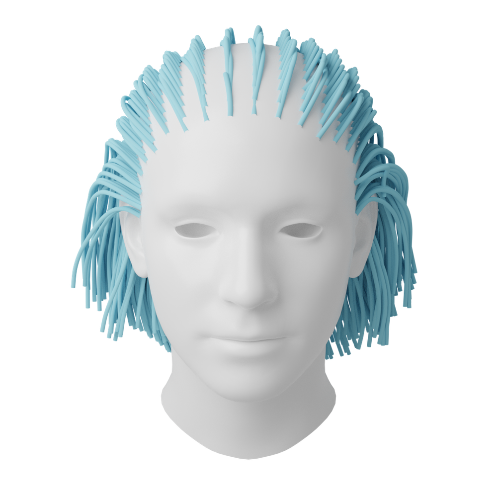
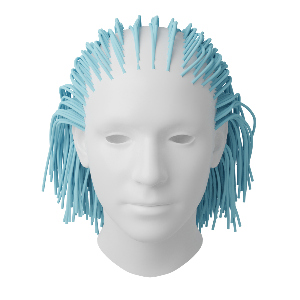
PCA	StyleGAN2	Ground Truth

Figure 6. Comparison of PCA and StyleGAN2 in reconstructing given guide strands.

4.1.3. Guide Interpolation

In Fig. 7 we compare the strands decoded from textures upsampled with different interpolation methods. Nearest neighbor interpolation ($2$nd column) produces aliased strands as it involves simple repetition. Bilinear interpolation ($3$rd column) leads to smoother strands, but introduces unwanted flyaway fibers, particularly in the forehead area. Our method ($5$th column) achieves the most natural result, which resembles the shape of guide strands and forms reasonable hair partitions. In addition, we employ the same U-Net architecture but configure it to directly predict strand PCA coefficients rather than the blending weights. The output ($4$th column) contains more flyaway strands and a reduced fidelity in capturing the overall hair shape, particularly noticeable in the lower part of the hair.

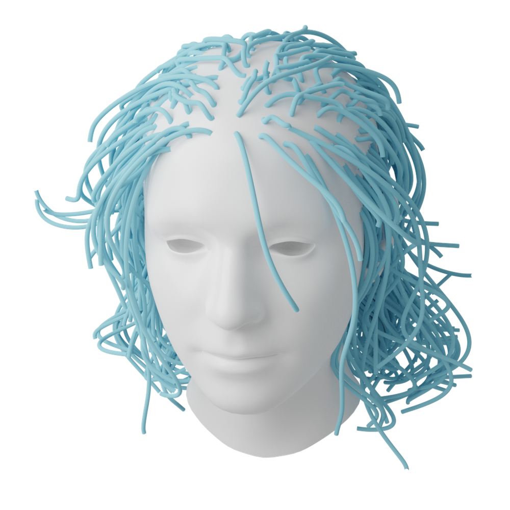
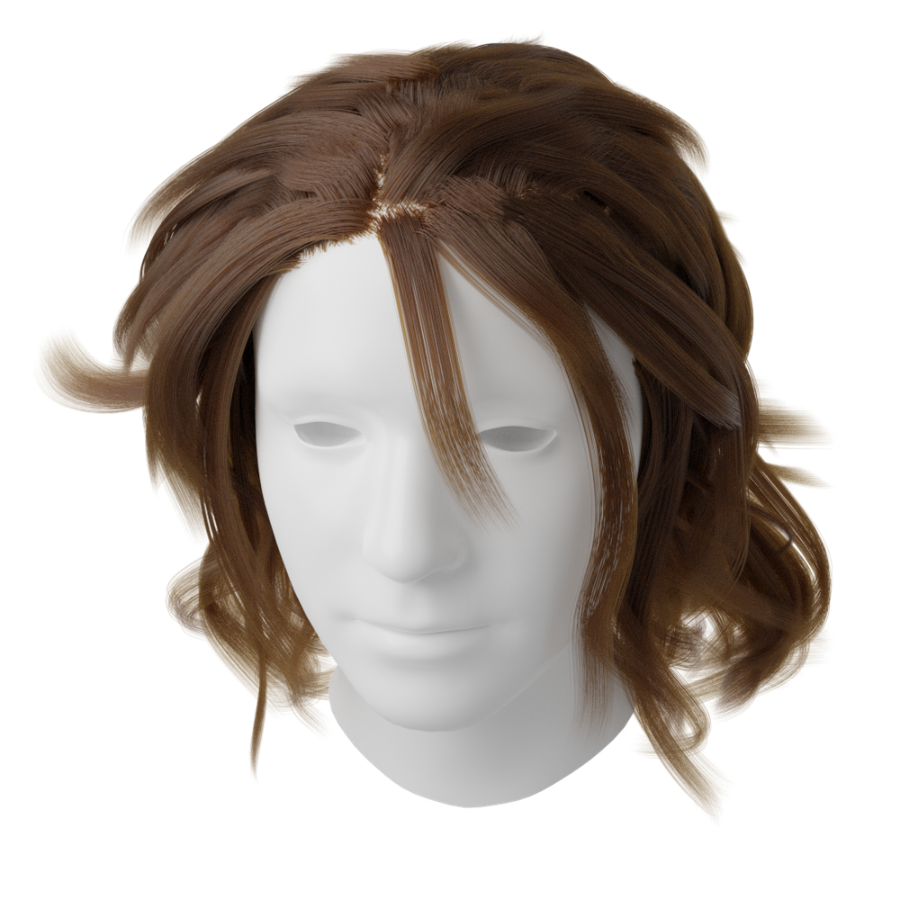
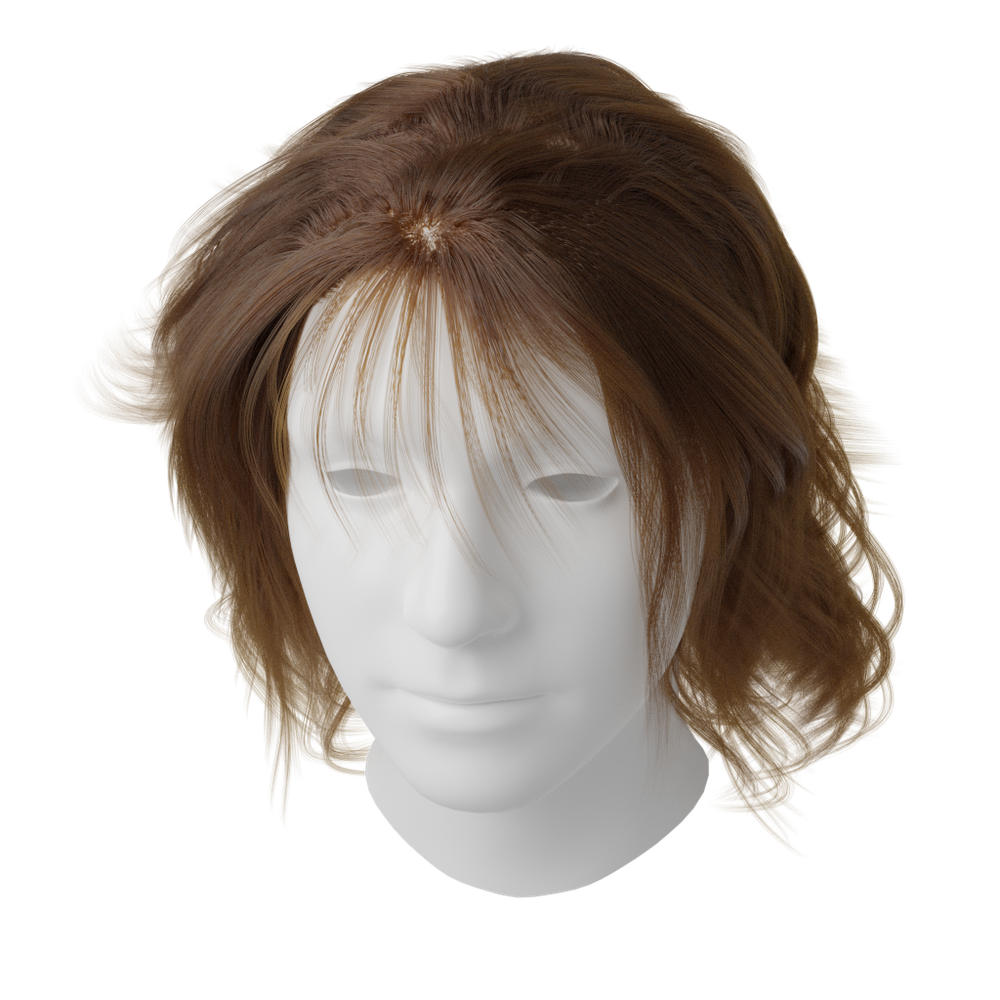
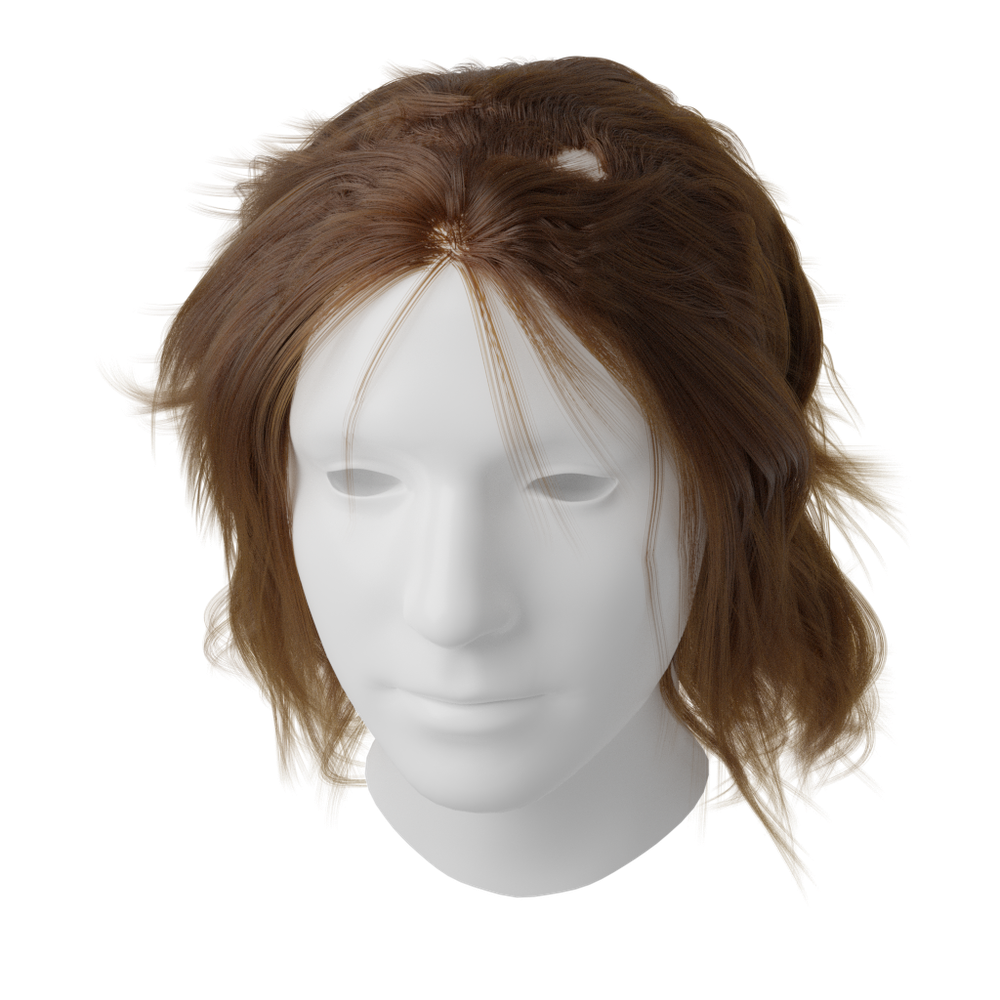
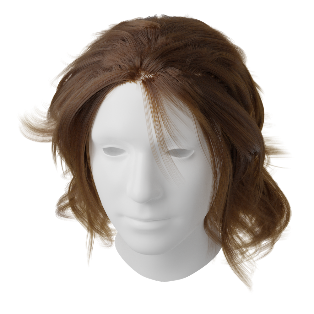
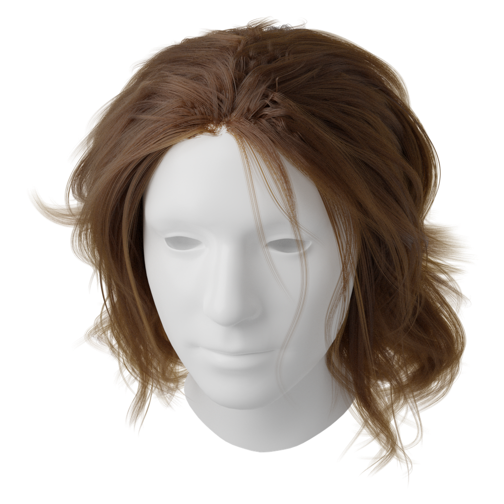
Guide Strands	Nearest	Bilinear	U-Net (coeff.)	Ours	Ground Truth

Figure 7. Comparison of strands upsampled with different interpolation methods.

4.1.4. Hair Styling

For the hair styling module, though StyleGAN2 performed well in synthesizing guide strands, we found it collapsed to produce blurry residual textures when embedding them into the latent space, as shown in Fig. 8 (left). We conjecture that this issue may be attributed to the large size of residual textures ($256\times 256\times 54$), as they contain more data than high-resolution RGB images ($1024\times 1024\times 3$). Moreover, our dataset is smaller than those image datasets used for StyleGAN training (e.g., FFHQ [Karras et al., 2019], which contains $70$K high-quality portrait images), thus further suppressing the expressiveness of StyleGAN2. Considering these constraints, we devised our network architecture as a VAE, trading some sampling diversity for higher reconstruction fidelity, which reconstructs sharper residual textures (Fig. 8 middle).

StyleGAN2	VAE	Ground Truth

Figure 8. Reconstruction quality of embedding residual textures into the latent space of different network architectures.

4.1.5. Comparison with GroomGen

The most relevant previous work is GroomGen [Zhou et al., 2023] that learns hierarchical representations of 3D hair. Since there is no publicly available GroomGen code, we implemented and trained it on the same augmented USC-HairSalon dataset. Unlike image synthesis tasks, there are no standard metrics like FID to evaluate the quality of randomly synthesized 3D hair. Therefore, we focus our quantitative comparison on reconstruction tasks, specifically examining the reconstruction capabilities of different strand representations and model representations. In Table 1 ($2$nd and $4$th columns), we present quantitative comparison between our PCA-based strand representation and GroomGen’s VAE-based strand representation, indicating that our representation achieves a significantly better reconstruction with slightly higher curvature errors. To compare model representations, we embed hair geometry textures into the latent spaces, and report quantitative reconstruction errors in Table 2 ($3$rd and $4$th columns), where our method achieves both smaller position and curvature errors. Note that we do not evaluate reconstruction errors on guide strands, as our guide strand definition is different (we model smoothed guide strands without high-frequency curliness). For qualitative comparison, we randomly synthesize $10$ hairstyles by sampling our parameter space and GroomGen’s latent space with the same Gaussian noise, and visualize the results in Fig. 5 of our supplemental. In this comparison, most of our synthesized hairstyles look more natural compared to GroomGen’s results. More details of random hairstyle synthesis can be found in Supplemental C.2.

4.2. Applications

After training Perm, we can deploy it as a generic hair prior to solve different down-stream tasks.

4.2.1. 3D Hair Parameterization

The first application we explored is to fit Perm parameters to target 3D hair models through differentiable optimization, which we term as 3D hair parameterization. Technical details are provided in Supplemental C.3. In Fig. 9 we show a subset of fitted results. Even if the target hair model has no guide strands, our model can generate reasonable guide strands to depict their overall shapes, which can be obtained from $\mathcal{S}\big{(}\mathcal{G}(\vec{\theta}^{\ast})\big{)}$.

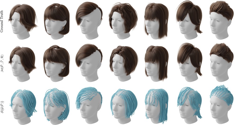
Figure 9. A subset of 3D hair models fitted by Perm. More results are available in Fig. 6 of our supplemental.

4.2.2. Hairstyle Interpolation

As we introduce separate parameters to control the global hair shape and local strand details, we can edit the hairstyle with varying granularity by interpolating the corresponding parameters. In the top row of Fig. 10, we linearly interpolate the guide strand parameter $\vec{\theta}$, resulting in hairstyles with different global shapes. Since the hair styling parameter $\vec{\beta}$ is kept fixed, local strand details, such as curls at the tips of strands, remain consistent. In the middle row, we fix the parameter $\vec{\theta}$ and linearly interpolate the parameter $\vec{\beta}$, thereby generating novel hairstyles ranging from straight to curly while maintaining a nearly identical global shape. In the bottom row, we jointly interpolate $\vec{\theta}$ and $\vec{\beta}$, demonstrating the transition from a short wavy hairstyle to a long straight hairstyle. The comparison with [Weng et al., 2013] and [Zhou et al., 2018] are provided in Supplemental C.4.

Interpolate $\vec{\theta}$ Only
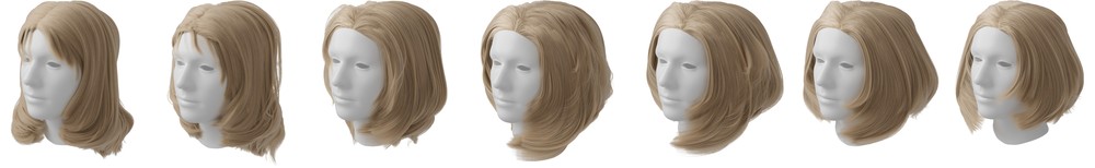
Interpolate $\vec{\beta}$ Only
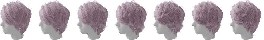
Joint Interpolation

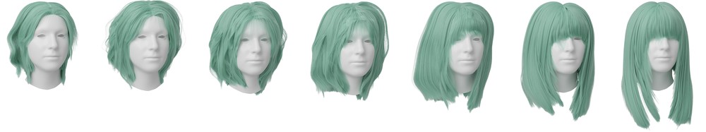
Figure 10. Hairstyle interpolation with different granularity. Top: interpolate $\vec{\theta}$ only and keep $\vec{\beta}$ fixed; Middle: interpolate $\vec{\beta}$ only and keep $\vec{\theta}$ fixed; Bottom: jointly interpolate $\vec{\theta}$ and $\vec{\beta}$.

4.2.3. Single-view Hair Reconstruction

With 2D observations as input, we can reconstruct 3D hair by optimizing Perm parameters to minimize the energy of generated hair when projected to the 2D images. Technical details are provided in Supplemental C.5. In Fig. 11 and Fig. 9 of our supplemental, we qualitatively compare our single-view reconstruction results with HairStep [Zheng et al., 2023], the state-of-the-art open-source method for single-view hair reconstruction. Our method not only excels in reconstructing the global shape of the reference hairstyle but also preserves local details better compared to HairStep. We also observed that HairStep occasionally generates unintended bald areas, while ours do not.

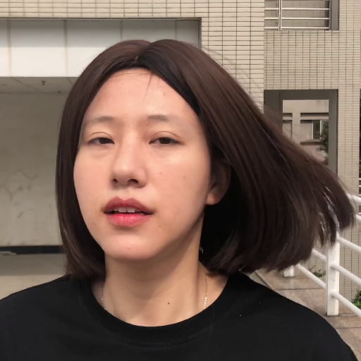
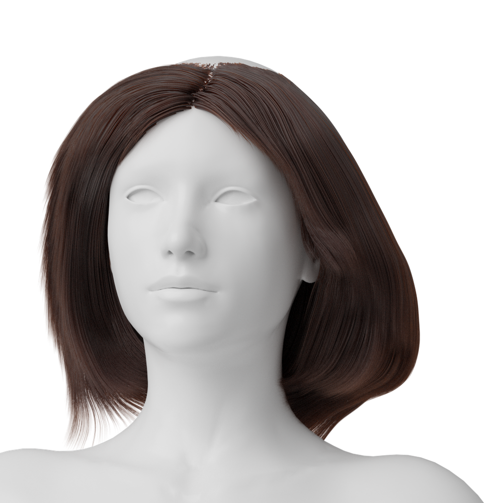
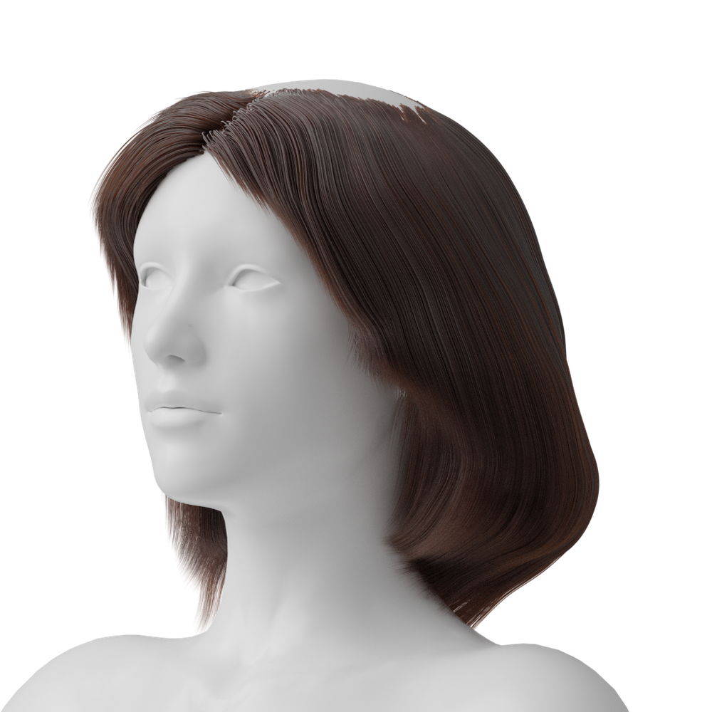
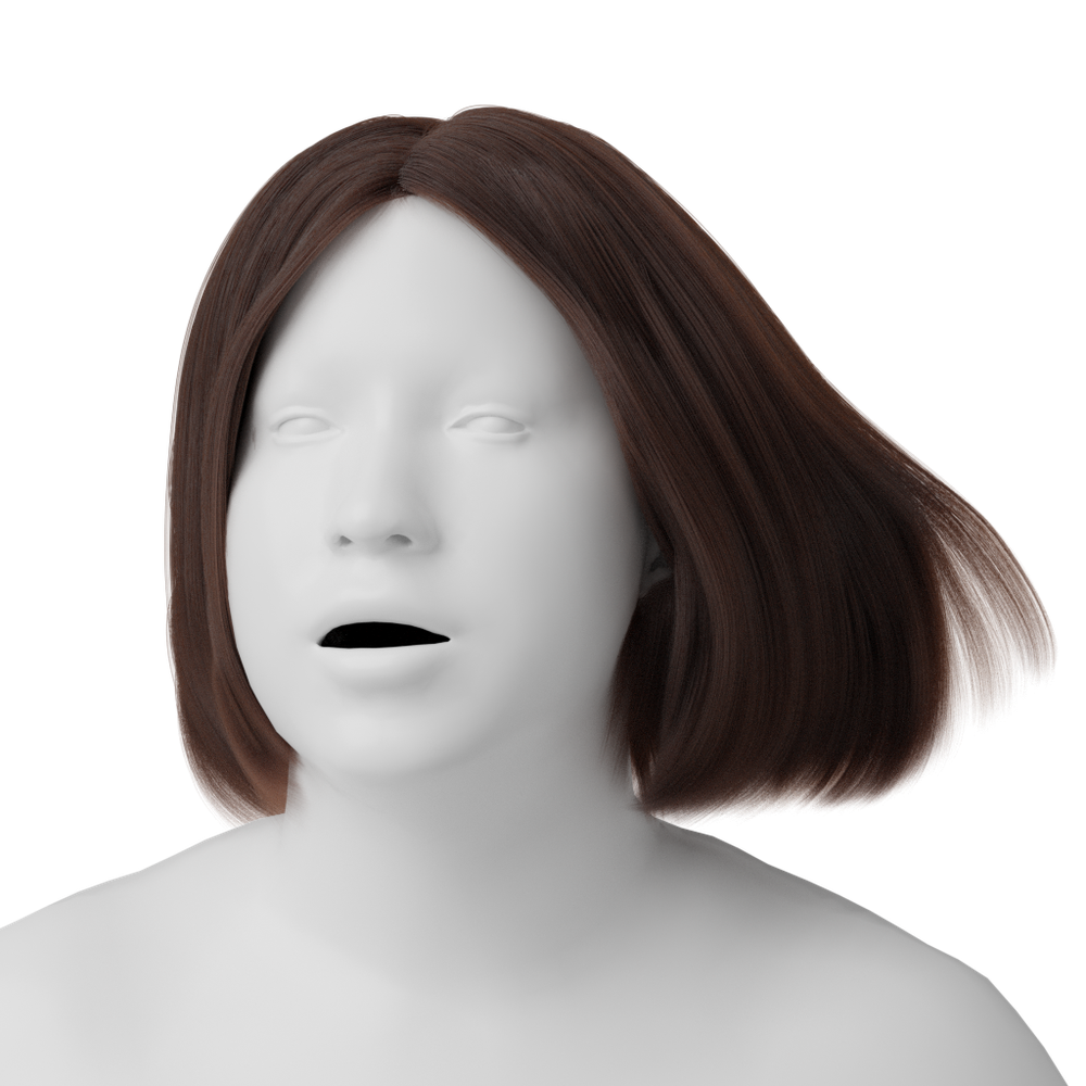
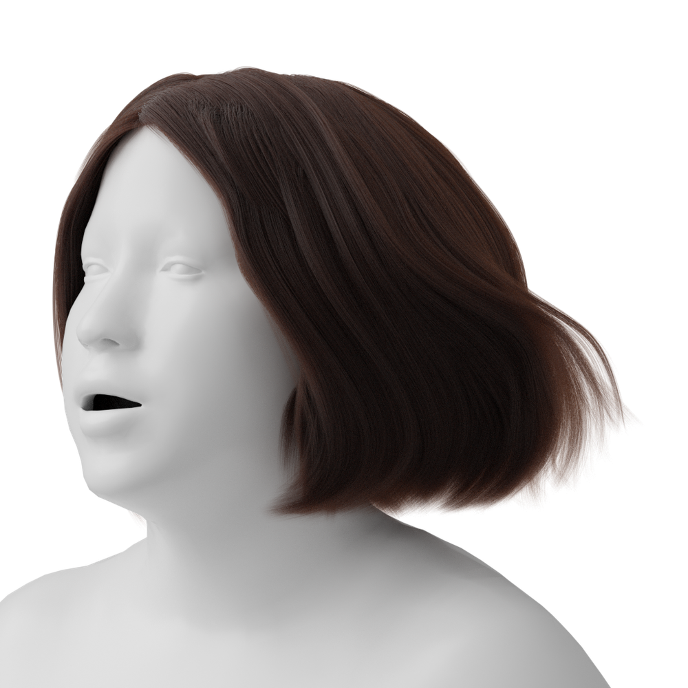
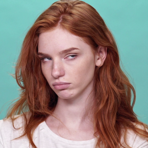
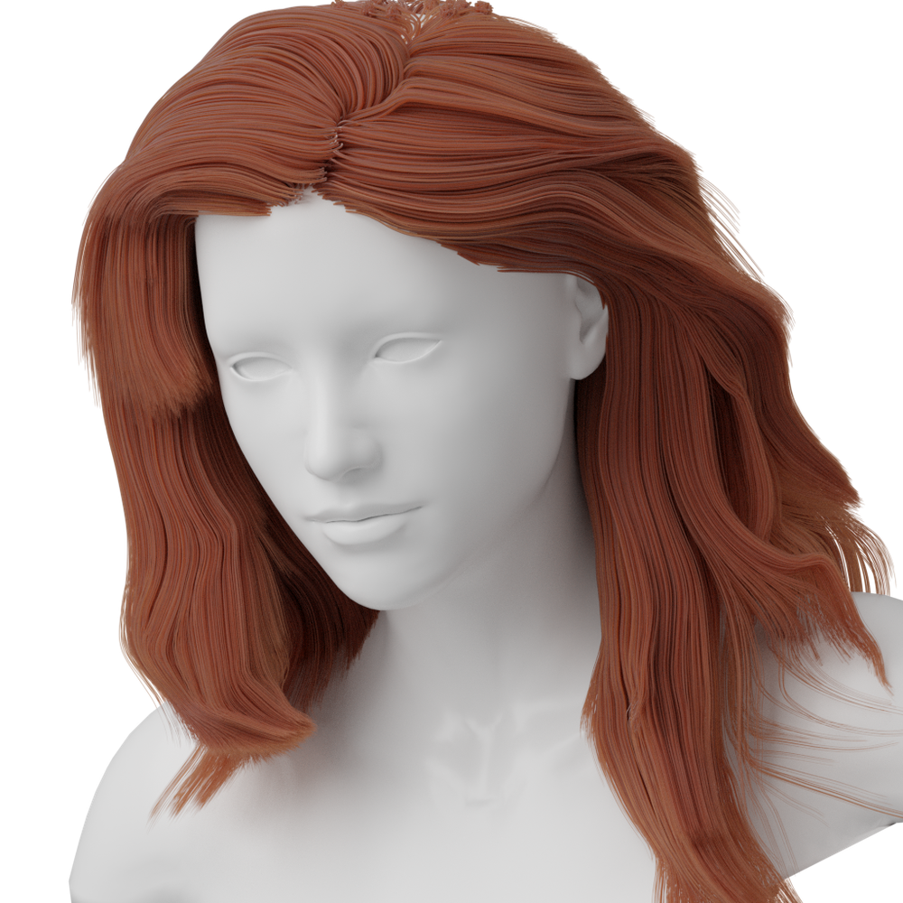
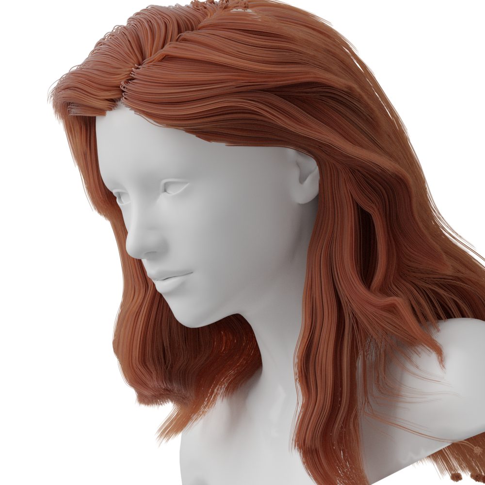
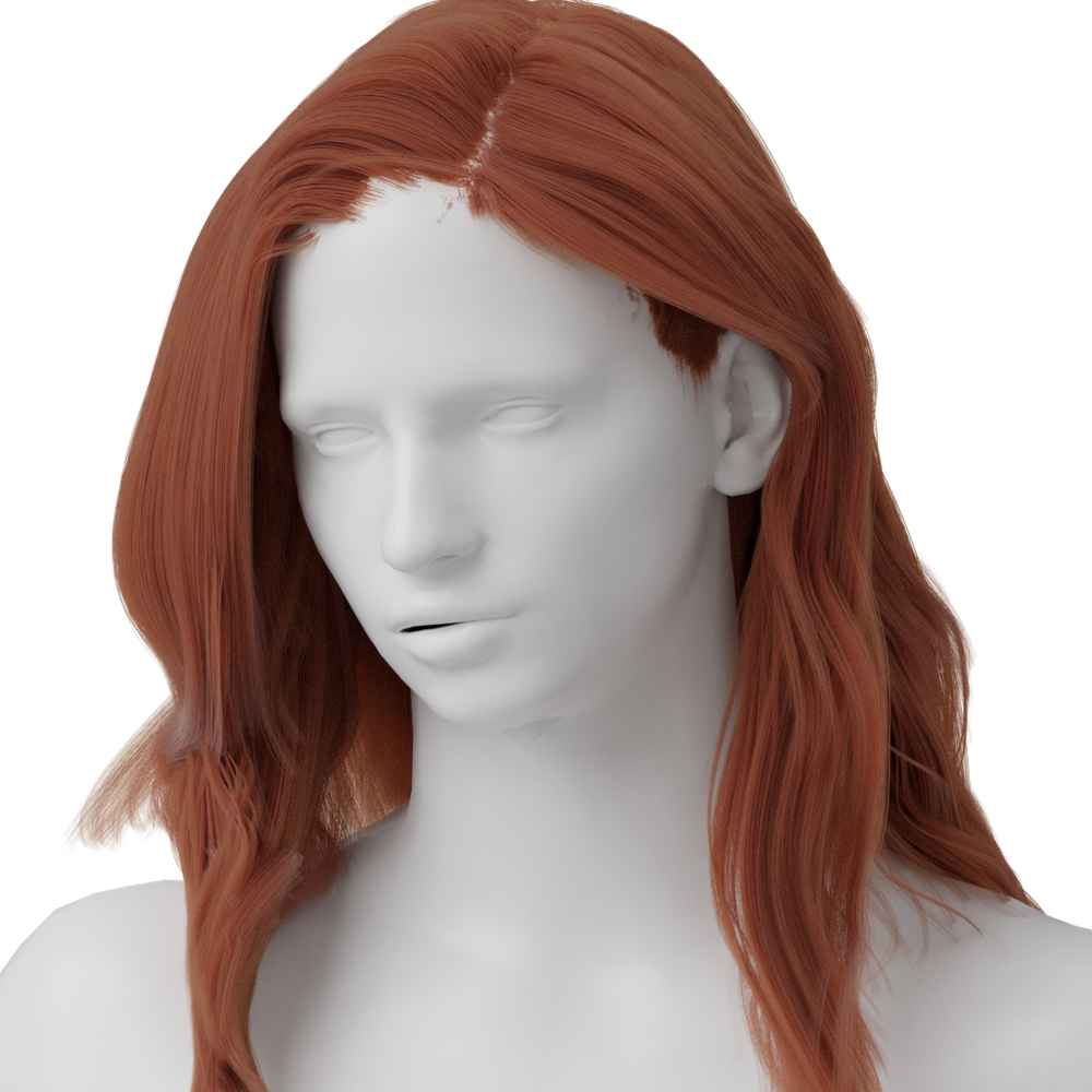
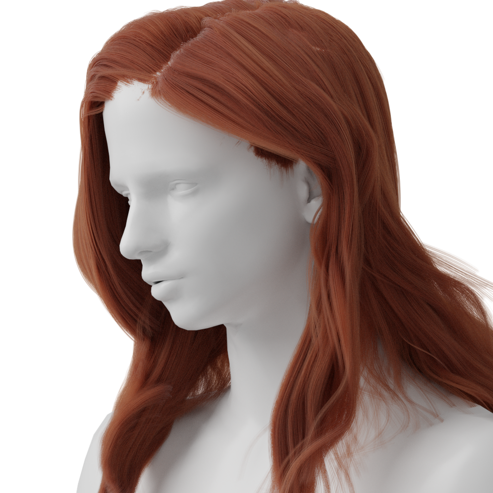
Input Image	HairStep [Zheng et al., 2023]		Ours

Figure 11. Qualitative comparison on single-view hair reconstruction with HairStep [Zheng et al., 2023]. More comparisons are provided in Fig. 9 and Fig. 10 of our supplemental.

4.2.4. Hair-conditioned Image Generation

Latest text-to-image (T2I) models (e.g., Adobe Firefly [Adobe, 2024]) can generate high-quality portrait images. However, the text embedding of simple prompts like “wavy and short hair” is not precise enough to represent a specific hairstyle. To tackle this issue, we show the use of Perm in facilitating conditional image generation. Specifically, We could use Perm to sample and edit hairstyles in 3D, or reconstruct 3D hairstyles from images, and then feed the depth and edge information extracted from the hair geometry to the T2I models to generate the final images. As shown in Fig. 11 of our supplemental, pure text prompts often lead to images with different hairstyles, while combined with the input hair reference, the generated images show a much more consistent hairstyle. More examples are available in Fig. 12 of our supplemental.

5. Limitations and Future Work

First, while our model adeptly fits and samples a diverse range of hairstyles, it currently faces challenges with intricate styles like buns and braids, as these complex hairstyles do not exist in the training data. Addressing this issue necessitates a systematic framework to efficiently capture a diverse set of real data. To this end, Perm can serve as a pre-trained prior for efficient data capture, as it can fill invisible parts of the hair, such as the interior and occluded regions, and accommodate more sparse image inputs. The captured hairs could also be used to fine-tune Perm to narrow the modal gap from real hairs. Moreover, aligning with trends in other 2D or 3D generative tasks, controllable 3D hair synthesis with multi-modal input signals (e.g., semantic attributes, natural languages, face parsing images, depth or normal maps, etc.) would be another promising direction to explore in our scenario.

References

- [1]
- Abdal et al. [2019] Rameen Abdal, Yipeng Qin, and Peter Wonka. 2019. Image2StyleGAN: How to Embed Images Into the StyleGAN Latent Space?. In Proceedings of the IEEE/CVF International Conference on Computer Vision (ICCV).
- Adobe [2024] Adobe. 2024. Firefly. https://www.adobe.com/products/firefly.html.
- Allen et al. [2003] Brett Allen, Brian Curless, and Zoran Popović. 2003. The space of human body shapes: reconstruction and parameterization from range scans. ACM transactions on graphics (TOG) 22, 3 (2003), 587–594.
- Autodesk [2024] Autodesk. 2024. Maya. https://www.autodesk.com/products/maya/.
- Blanz and Vetter [1999] Volker Blanz and Thomas Vetter. 1999. A morphable model for the synthesis of 3D faces. In Proceedings of the 26th annual conference on Computer graphics and interactive techniques. 187–194.
- Cao et al. [2014] Chen Cao, Yanlin Weng, Shun Zhou, Yiying Tong, and Kun Zhou. 2014. FaceWarehouse: A 3D Facial Expression Database for Visual Computing. IEEE Transactions on Visualization and Computer Graphics 20, 3 (2014), 413–425. https://doi.org/10.1109/TVCG.2013.249
- Chai et al. [2016a] Menglei Chai, Tianjia Shao, Hongzhi Wu, Yanlin Weng, and Kun Zhou. 2016a. AutoHair: Fully Automatic Hair Modeling from a Single Image. 35, 4, Article 116 (jul 2016), 12 pages. https://doi.org/10.1145/2897824.2925961
- Chai et al. [2013] Menglei Chai, Lvdi Wang, Yanlin Weng, Xiaogang Jin, and Kun Zhou. 2013. Dynamic hair manipulation in images and videos. ACM Transactions on Graphics (TOG) 32, 4 (2013), 1–8.
- Chai et al. [2012] Menglei Chai, Lvdi Wang, Yanlin Weng, Yizhou Yu, Baining Guo, and Kun Zhou. 2012. Single-view hair modeling for portrait manipulation. ACM Transactions on Graphics (TOG) 31, 4 (2012), 1–8.
- Chai et al. [2014] Menglei Chai, Changxi Zheng, and Kun Zhou. 2014. A reduced model for interactive hairs. ACM Transactions on Graphics (TOG) 33, 4 (2014), 1–11.
- Chai et al. [2016b] Menglei Chai, Changxi Zheng, and Kun Zhou. 2016b. Adaptive skinning for interactive hair-solid simulation. IEEE transactions on visualization and computer graphics 23, 7 (2016), 1725–1738.
- Chan et al. [2022] Eric R. Chan, Connor Z. Lin, Matthew A. Chan, Koki Nagano, Boxiao Pan, Shalini De Mello, Orazio Gallo, Leonidas Guibas, Jonathan Tremblay, Sameh Khamis, Tero Karras, and Gordon Wetzstein. 2022. Efficient Geometry-aware 3D Generative Adversarial Networks. In CVPR.
- Chen et al. [1999] Lieu-Hen Chen, Santi Saeyor, Hiroshi Dohi, and Mitsuru Ishizuka. 1999. A system of 3d hair style synthesis based on the wisp model. The Visual Computer 15 (1999), 159–170.
- Fu et al. [2007] Hongbo Fu, Yichen Wei, Chiew-Lan Tai, and Long Quan. 2007. Sketching hairstyles. In Proceedings of the 4th Eurographics workshop on Sketch-based interfaces and modeling. 31–36.
- Goodfellow et al. [2014] Ian Goodfellow, Jean Pouget-Abadie, Mehdi Mirza, Bing Xu, David Warde-Farley, Sherjil Ozair, Aaron Courville, and Yoshua Bengio. 2014. Generative adversarial nets. Advances in neural information processing systems 27 (2014).
- Grabli et al. [2002] Stéphane Grabli, François X Sillion, Stephen R Marschner, and Jerome E Lengyel. 2002. Image-based hair capture by inverse lighting. In Proceedings of Graphics Interface (GI). 51–58.
- Herrera et al. [2012] Tomas Lay Herrera, Arno Zinke, and Andreas Weber. 2012. Lighting Hair from the inside: A Thermal Approach to Hair Reconstruction. ACM Trans. Graph. 31, 6, Article 146 (nov 2012), 9 pages. https://doi.org/10.1145/2366145.2366165
- Hesse et al. [2018] Nikolas Hesse, Sergi Pujades, Javier Romero, Michael J Black, Christoph Bodensteiner, Michael Arens, Ulrich G Hofmann, Uta Tacke, Mijna Hadders-Algra, Raphael Weinberger, et al. 2018. Learning an infant body model from RGB-D data for accurate full body motion analysis. In Medical Image Computing and Computer Assisted Intervention–MICCAI 2018: 21st International Conference, Granada, Spain, September 16-20, 2018, Proceedings, Part I. Springer, 792–800.
- Ho et al. [2020] Jonathan Ho, Ajay Jain, and Pieter Abbeel. 2020. Denoising diffusion probabilistic models. Advances in neural information processing systems 33 (2020), 6840–6851.
- Hu et al. [2014] Liwen Hu, Chongyang Ma, Linjie Luo, and Hao Li. 2014. Robust hair capture using simulated examples. ACM Transactions on Graphics (TOG) 33, 4 (2014), 1–10.
- Hu et al. [2015] Liwen Hu, Chongyang Ma, Linjie Luo, and Hao Li. 2015. Single-View Hair Modeling Using A Hairstyle Database. ACM Transactions on Graphics (Proceedings SIGGRAPH 2015) 34, 4 (July 2015).
- Jakob et al. [2009] Wenzel Jakob, Jonathan T Moon, and Steve Marschner. 2009. Capturing hair assemblies fiber by fiber. In ACM SIGGRAPH Asia 2009 papers. 1–9.
- Karras et al. [2019] Tero Karras, Samuli Laine, and Timo Aila. 2019. A style-based generator architecture for generative adversarial networks. In Proceedings of the IEEE/CVF conference on computer vision and pattern recognition. 4401–4410.
- Karras et al. [2020] Tero Karras, Samuli Laine, Miika Aittala, Janne Hellsten, Jaakko Lehtinen, and Timo Aila. 2020. Analyzing and Improving the Image Quality of StyleGAN. In Proc. CVPR.
- Kim and Neumann [2002] Tae-Yong Kim and Ulrich Neumann. 2002. Interactive multiresolution hair modeling and editing. ACM Transactions on Graphics (TOG) 21, 3 (2002), 620–629.
- Kingma and Welling [2013] Diederik P Kingma and Max Welling. 2013. Auto-encoding variational bayes. arXiv preprint arXiv:1312.6114 (2013).
- Kuang et al. [2022] Zhiyi Kuang, Yiyang Chen, Hongbo Fu, Kun Zhou, and Youyi Zheng. 2022. DeepMVSHair: Deep Hair Modeling from Sparse Views. In SIGGRAPH Asia 2022 Conference Papers. Article 10, 8 pages.
- Li et al. [2017] Tianye Li, Timo Bolkart, Michael. J. Black, Hao Li, and Javier Romero. 2017. Learning a model of facial shape and expression from 4D scans. ACM Transactions on Graphics, (Proc. SIGGRAPH Asia) 36, 6 (2017), 194:1–194:17. https://doi.org/10.1145/3130800.3130813
- Liang et al. [2018] Shu Liang, Xiufeng Huang, Xianyu Meng, Kunyao Chen, Linda G Shapiro, and Ira Kemelmacher-Shlizerman. 2018. Video to fully automatic 3d hair model. ACM Transactions on Graphics (TOG) 37, 6 (2018), 1–14.
- Loper et al. [2015] Matthew Loper, Naureen Mahmood, Javier Romero, Gerard Pons-Moll, and Michael J. Black. 2015. SMPL: A Skinned Multi-Person Linear Model. ACM Trans. Graphics (Proc. SIGGRAPH Asia) 34, 6 (Oct. 2015), 248:1–248:16.
- Luo et al. [2024] Haimin Luo, Min Ouyang, Zijun Zhao, Suyi Jiang, Longwen Zhang, Qixuan Zhang, Wei Yang, Lan Xu, and Jingyi Yu. 2024. GaussianHair: Hair Modeling and Rendering with Light-aware Gaussians. arXiv preprint arXiv:2402.10483 (2024).
- Luo et al. [2013] Linjie Luo, Hao Li, and Szymon Rusinkiewicz. 2013. Structure-aware hair capture. ACM Transactions on Graphics (TOG) 32, 4 (2013), 1–12.
- Luo et al. [2023] Zhongjin Luo, Shengcai Cai, Jinguo Dong, Ruibo Ming, Liangdong Qiu, Xiaohang Zhan, and Xiaoguang Han. 2023. RaBit: Parametric Modeling of 3D Biped Cartoon Characters with a Topological-consistent Dataset. arXiv preprint arXiv:2303.12564 (2023).
- Lyu et al. [2020] Qing Lyu, Menglei Chai, Xiang Chen, and Kun Zhou. 2020. Real-time hair simulation with neural interpolation. IEEE Transactions on Visualization and Computer Graphics 28, 4 (2020), 1894–1905.
- Mescheder et al. [2018] Lars Mescheder, Andreas Geiger, and Sebastian Nowozin. 2018. Which training methods for GANs do actually converge?. In International conference on machine learning. PMLR, 3481–3490.
- Nam et al. [2019] Giljoo Nam, Chenglei Wu, Min H. Kim, and Yaser Sheikh. 2019. Strand-Accurate Multi-View Hair Capture. In 2019 IEEE/CVF Conference on Computer Vision and Pattern Recognition (CVPR). 155–164. https://doi.org/10.1109/CVPR.2019.00024
- Paris et al. [2004] Sylvain Paris, Hector M. Briceño, and François X. Sillion. 2004. Capture of hair geometry from multiple images. ACM Trans. Graph. 23, 3 (aug 2004), 712–719.
- Pavlakos et al. [2019] Georgios Pavlakos, Vasileios Choutas, Nima Ghorbani, Timo Bolkart, Ahmed AA Osman, Dimitrios Tzionas, and Michael J Black. 2019. Expressive body capture: 3d hands, face, and body from a single image. In Proceedings of the IEEE/CVF conference on computer vision and pattern recognition. 10975–10985.
- Richardson et al. [2021] Elad Richardson, Yuval Alaluf, Or Patashnik, Yotam Nitzan, Yaniv Azar, Stav Shapiro, and Daniel Cohen-Or. 2021. Encoding in Style: a StyleGAN Encoder for Image-to-Image Translation. In IEEE/CVF Conference on Computer Vision and Pattern Recognition (CVPR).
- Romero et al. [2017] Javier Romero, Dimitrios Tzionas, and Michael J. Black. 2017. Embodied Hands: Modeling and Capturing Hands and Bodies Together. ACM Transactions on Graphics, (Proc. SIGGRAPH Asia) 36, 6 (Nov. 2017).
- Ronneberger et al. [2015] Olaf Ronneberger, Philipp Fischer, and Thomas Brox. 2015. U-net: Convolutional networks for biomedical image segmentation. In Medical Image Computing and Computer-Assisted Intervention–MICCAI 2015: 18th International Conference, Munich, Germany, October 5-9, 2015, Proceedings, Part III 18. Springer, 234–241.
- Rosu et al. [2022] Radu Alexandru Rosu, Shunsuke Saito, Ziyan Wang, Chenglei Wu, Sven Behnke, and Giljoo Nam. 2022. Neural Strands: Learning Hair Geometry and Appearance from Multi-View Images. ECCV (2022).
- Saito et al. [2018] Shunsuke Saito, Liwen Hu, Chongyang Ma, Hikaru Ibayashi, Linjie Luo, and Hao Li. 2018. 3D Hair Synthesis Using Volumetric Variational Autoencoders. ACM Trans. Graph. 37, 6, Article 208 (dec 2018), 12 pages. https://doi.org/10.1145/3272127.3275019
- Shen et al. [2023] Yuefan Shen, Shunsuke Saito, Ziyan Wang, Olivier Maury, Chenglei Wu, Jessica Hodgins, Youyi Zheng, and Giljoo Nam. 2023. CT2Hair: High-Fidelity 3D Hair Modeling using Computed Tomography. ACM Transactions on Graphics 42, 4 (2023), 1–13.
- Shen et al. [2020] Yuefan Shen, Changgeng Zhang, Hongbo Fu, Kun Zhou, and Youyi Zheng. 2020. Deepsketchhair: Deep sketch-based 3d hair modeling. IEEE transactions on visualization and computer graphics 27, 7 (2020), 3250–3263.
- Sklyarova et al. [2023a] Vanessa Sklyarova, Jenya Chelishev, Andreea Dogaru, Igor Medvedev, Victor Lempitsky, and Egor Zakharov. 2023a. Neural Haircut: Prior-Guided Strand-Based Hair Reconstruction. In Proceedings of IEEE International Conference on Computer Vision (ICCV).
- Sklyarova et al. [2023b] Vanessa Sklyarova, Egor Zakharov, Otmar Hilliges, Michael J Black, and Justus Thies. 2023b. HAAR: Text-Conditioned Generative Model of 3D Strand-based Human Hairstyles. ArXiv (Dec 2023).
- Takimoto et al. [2024] Yusuke Takimoto, Hikari Takehara, Hiroyuki Sato, Zihao Zhu, and Bo Zheng. 2024. Dr. Hair: Reconstructing Scalp-Connected Hair Strands without Pre-training via Differentiable Rendering of Line Segments. arXiv preprint arXiv:2403.17496 (2024).
- Wang et al. [2009] Lvdi Wang, Yizhou Yu, Kun Zhou, and Baining Guo. 2009. Example-Based Hair Geometry Synthesis. In ACM SIGGRAPH 2009 Papers (New Orleans, Louisiana) (SIGGRAPH ’09). Association for Computing Machinery, New York, NY, USA, Article 56, 9 pages. https://doi.org/10.1145/1576246.1531362
- Wang et al. [2023a] Ziyan Wang, Giljoo Nam, Aljaz Bozic, Chen Cao, Jason Saragih, Michael Zollhoefer, and Jessica Hodgins. 2023a. A Local Appearance Model for Volumetric Capture of Diverse Hairstyle. arXiv preprint arXiv:2312.08679 (2023).
- Wang et al. [2023b] Ziyan Wang, Giljoo Nam, Tuur Stuyck, Stephen Lombardi, Chen Cao, Jason Saragih, Michael Zollhöfer, Jessica Hodgins, and Christoph Lassner. 2023b. NeuWigs: A Neural Dynamic Model for Volumetric Hair Capture and Animation. In Proceedings of the IEEE/CVF Conference on Computer Vision and Pattern Recognition. 8641–8651.
- Wang et al. [2022] Ziyan Wang, Giljoo Nam, Tuur Stuyck, Stephen Lombardi, Michael Zollhöfer, Jessica Hodgins, and Christoph Lassner. 2022. HVH: Learning a Hybrid Neural Volumetric Representation for Dynamic Hair Performance Capture. In Proceedings of the IEEE/CVF Conference on Computer Vision and Pattern Recognition. 6143–6154.
- Watanabe and Suenaga [1992] Yasuhiko Watanabe and Yasuhito Suenaga. 1992. A trigonal prism-based method for hair image generation. IEEE Computer Graphics and applications 12, 01 (1992), 47–53.
- Wei et al. [2005] Yichen Wei, Eyal Ofek, Long Quan, and Heung-Yeung Shum. 2005. Modeling hair from multiple views. In ACM SIGGRAPH 2005 Papers (SIGGRAPH ’05). 816–820.
- Weng et al. [2013] Yanlin Weng, Lvdi Wang, Xiao Li, Menglei Chai, and Kun Zhou. 2013. Hair interpolation for portrait morphing. In Computer Graphics Forum, Vol. 32. 79–84.
- Wu et al. [2024] Keyu Wu, Lingchen Yang, Zhiyi Kuang, Yao Feng, Xutao Han, Yuefan Shen, Hongbo Fu, Kun Zhou, and Youyi Zheng. 2024. MonoHair: High-Fidelity Hair Modeling from a Monocular Video. arXiv preprint arXiv:2403.18356 (2024).
- Wu et al. [2022] Keyu Wu, Yifan Ye, Lingchen Yang, Hongbo Fu, Kun Zhou, and Youyi Zheng. 2022. NeuralHDHair: Automatic High-fidelity Hair Modeling from a Single Image Using Implicit Neural Representations. In Proceedings of the IEEE/CVF Conference on Computer Vision and Pattern Recognition. 1526–1535.
- Xing et al. [2019] Jun Xing, Koki Nagano, Weikai Chen, Haotian Xu, Li-yi Wei, Yajie Zhao, Jingwan Lu, Byungmoon Kim, and Hao Li. 2019. Hairbrush for immersive data-driven hair modeling. In Proceedings of the 32Nd Annual ACM Symposium on User Interface Software and Technology. 263–279.
- Xu et al. [2014] Zexiang Xu, Hsiang-Tao Wu, Lvdi Wang, Changxi Zheng, Xin Tong, and Yue Qi. 2014. Dynamic hair capture using spacetime optimization. 33, 6, Article 224 (nov 2014), 11 pages.
- Yang et al. [2019] Lingchen Yang, Zefeng Shi, Youyi Zheng, and Kun Zhou. 2019. Dynamic hair modeling from monocular videos using deep neural networks. ACM Transactions on Graphics (TOG) 38, 6 (2019), 1–12.
- Yuksel et al. [2009] Cem Yuksel, Scott Schaefer, and John Keyser. 2009. Hair meshes. ACM Transactions on Graphics (TOG) 28, 5 (2009), 1–7.
- Zhang et al. [2017] Meng Zhang, Menglei Chai, Hongzhi Wu, Hao Yang, and Kun Zhou. 2017. A data-driven approach to four-view image-based hair modeling. ACM Trans. Graph. 36, 4 (2017), 156–1.
- Zhang et al. [2018] Meng Zhang, Pan Wu, Hongzhi Wu, Yanlin Weng, Youyi Zheng, and Kun Zhou. 2018. Modeling hair from an rgb-d camera. ACM Transactions on Graphics (TOG) 37, 6 (2018), 1–10.
- Zhang and Zheng [2019] Meng Zhang and Youyi Zheng. 2019. Hair-GAN: Recovering 3D hair structure from a single image using generative adversarial networks. Visual Informatics 3, 2 (2019), 102–112.
- Zheng et al. [2023] Yujian Zheng, Zirong Jin, Moran Li, Haibin Huang, Chongyang Ma, Shuguang Cui, and Xiaoguang Han. 2023. HairStep: Transfer Synthetic to Real Using Strand and Depth Maps for Single-View 3D Hair Modeling. In Proceedings of the IEEE/CVF Conference on Computer Vision and Pattern Recognition.
- Zhou et al. [2023] Yuxiao Zhou, Menglei Chai, Alessandro Pepe, Markus Gross, and Thabo Beeler. 2023. GroomGen: A High-Quality Generative Hair Model Using Hierarchical Latent Representations. arXiv preprint arXiv:2311.02062 (2023).
- Zhou et al. [2018] Yi Zhou, Liwen Hu, Jun Xing, Weikai Chen, Han-Wei Kung, Xin Tong, and Hao Li. 2018. Hairnet: Single-view hair reconstruction using convolutional neural networks. In Proceedings of the European Conference on Computer Vision (ECCV). 235–251.
- Zuffi et al. [2017] Silvia Zuffi, Angjoo Kanazawa, David Jacobs, and Michael J. Black. 2017. 3D Menagerie: Modeling the 3D Shape and Pose of Animals. In IEEE Conf. on Computer Vision and Pattern Recognition (CVPR).