Piecewise deterministic generative models

Abstract

We introduce a novel class of generative models based on piecewise deterministic Markov processes (PDMPs), a family of non-diffusive stochastic processes consisting of deterministic motion and random jumps at random times. Similarly to diffusions, such Markov processes admit time reversals that turn out to be PDMPs as well. We apply this observation to three PDMPs considered in the literature: the Zig-Zag process, Bouncy Particle Sampler, and Randomised Hamiltonian Monte Carlo. For these three particular instances, we show that the jump rates and kernels of the corresponding time reversals admit explicit expressions depending on some conditional densities of the PDMP under consideration before and after a jump. Based on these results, we propose efficient training procedures to learn these characteristics and consider methods to approximately simulate the reverse process. Finally, we provide bounds in the total variation distance between the data distribution and the resulting distribution of our model in the case where the base distribution is the standard $d$-dimensional Gaussian distribution. Promising numerical simulations support further investigations into this class of models.

1 Introduction

Diffusion-based generative models (Ho et al., 2020; Song et al., 2021) have recently achieved state-of-the-art performance in various fields of application (Dhariwal and Nichol, 2021; Croitoru et al., 2023; Jeong et al., 2021; Kong et al., 2021). In their continuous time interpretation (Song et al., 2021), these models leverage the idea that a diffusion process can bridge the data distribution $\mu_{\star}$ to a base distribution $\pi$, and its time reversal can transform samples from $\pi$ into synthetic data from $\mu_{\star}$. As shown in the 1980s by Anderson (1982), the time reversal of a diffusion process, i.e., the backward process, is itself a diffusion with explicit drift and covariance functions that are related to the score functions of the time-marginal densities of the original, forward diffusion. Consequently, the key element of these generative models is learning these score functions using techniques such as (denoising) score-matching (Hyvärinen, 2005; Vincent, 2011).

In this work, we explore the potential of using piecewise deterministic Markov processes (PDMPs) as noising processes instead of diffusions. PDMPs were introduced around forty years ago (Davis, 1984, 1993) and since then have been successfully applied in various fields, including communication networks (Dumas et al., 2002), biology (Berg and Brown, 1972; Cloez, Bertrand et al., 2017), risk theory (Embrechts and Schmidli, 1994), and the reliability of complex systems (Zhang et al., 2008). More recently, PDMPs have been intensively studied in the context of Monte Carlo algorithms (Fearnhead et al., 2018) as alternatives to Langevin diffusion-based methods and Metropolis-Hastings mechanisms. This renewed interest in PDMPs has led to the development of novel processes, such as the Zig-Zag process (ZZP) (Bierkens et al., 2019a), the Bouncy Particle Sampler (BPS) (Bouchard-Côté et al., 2018), and the Randomised Hamiltonian Monte Carlo (RHMC) (Bou-Rabee and Sanz-Serna, 2017). Compared to Langevin-based methods, PDMPs offer several advantages, such as better scalability and reduced computational complexity in high-dimensional settings (Bierkens et al., 2019a).

In this paper, we propose a new family of generative models based on PDMPs. Our contributions are the following:

1. Leveraging the existing literature on time reversals of Markov jump processes (Conforti and Léonard, 2022), we characterise the time reversal of any PDMP under appropriate conditions. It turns out that this time reversal is itself a PDMP with characteristics related to the original PDMP; see Proposition 1.

2. We further specify the characteristics of the time-reversal processes associated with the three aforementioned PDMPs: ZZP, BPS, and RHMC. For these processes, Proposition 2 shows the corresponding time-reversals are PDMPs with simple reversed deterministic motion and with jump rates and kernels that depend on (ratios of) conditional densities of the velocity of the forward process before and after a jump. In contrast to common diffusion models, the emphasis is on distributions of the velocity, similar to the case of the underdamped Langevin diffusion (Dockhorn et al., 2022), which includes an additional velocity vector akin to the PDMPs we consider. Moreover, the structure of the backward jump rates and kernels closely connects to the case of continuous time jump processes on discrete state spaces (Sun et al., 2023; Lou et al., 2024).

3. We define our piecewise deterministic generative models employing either ZZP, BPS, or RHMC as forward process, transforming data points to a noise distribution of choice, and develop methodologies to estimate the backward rates and kernels. Then, we define the corresponding backward process based on approximations of the time reversed ZZP, BPS, and RHMC obtained with the estimated rates and kernels. In Section 4 we test our models on simple toy distributions.

4. We obtain a bound for the total variation distance between the data distribution and the distribution of our generative models taking into account two sources of error: first, the approximation of the characteristics of the backward PDMP, and second, its initialisation from the limiting distribution of the forward process; see Theorem 1.

2 PDMP based generative models

2.1 Piecewise deterministic Markov processes

Informally, a PDMP (Davis, 1984, 1993) on the measurable space $(\mathbb{R}^{D},\mathcal{B}(\mathbb{R}^{D}))$ is a stochastic process that follows deterministic dynamics between random times, while at these times, the process can evolve stochastically on the basis of a Markov kernel. In order to define a PDMP precisely, we need three components, which we call characteristics of the PDMP: a vector field $\Phi:\mathbb{R}_{+}\times\mathbb{R}^{D}\to\mathbb{R}^{D}$, which governs the deterministic motion, a jump rate $\lambda:\mathbb{R}_{+}\times\mathbb{R}^{D}\to\mathbb{R}_{+}$, which defines the law of random event times, and finally a jump kernel $Q:\mathbb{R}_{+}\times\mathbb{R}^{D}\times\mathcal{B}(\mathbb{R}^{D})\to[0,1]$, which is applied at event times and defines the new location of the process. Now we can describe the formal construction of a PDMP with the characteristics $(\Phi,\lambda,Q)$. To this end, consider the differential flow $\varphi:(t,s,z)\mapsto\varphi_{t,t+s}(z)$, which solves the ODE, $\mathrm{d}z_{t+s}=\Phi(t+s,z_{t+s})\mathrm{d}s$ for $s\geqslant 0$, i.e. $z_{t+s}=\varphi_{t,t+s}(z_{t})$. We define by recursion on $n\in\mathbb{N}$ the process on $(Z_{t})_{t\in\left[0,\mathrm{T}_{n}\right]}$ on $\left[0,\mathrm{T}_{n}\right]$ and the increasing sequence of jump times $(T_{n})_{n\in\mathbb{N}}$ starting from an initial state $Z_{0}$ and setting $\mathrm{T}_{0}=0$. Assume that $(\mathrm{T}_{i})_{i\in\{0,\ldots,n\}}$ and $(Z_{t})_{t\in\left[0,\mathrm{T}_{n}\right]}$ are defined for some $n\in\mathbb{N}$. We now define $(Z_{t})_{t\in\left[\mathrm{T}_{n},\mathrm{T}_{n+1}\right]}$. First, we define

$$\tau_{n+1}=\inf\left\{t>0:\int_{0}^{t}\lambda(T_{n}+u,\varphi_{\mathrm{T}_{n},\mathrm{T}_{n}+u}(Z_{\mathrm{T}_{n}}))\mathrm{d}u\geqslant E_{n+1}\right\}$$ (1)

where $E_{n+1}\sim\text{Exp}(1)$, and set the $n+1$-th jump time $\mathrm{T}_{n+1}=\mathrm{T}_{n}+\tau_{n+1}$. The process is then defined on $\left[\mathrm{T}_{n},\mathrm{T}_{n+1}\right)$ by $Z_{\mathrm{T}_{n}+t}=\varphi_{\mathrm{T}_{n},\mathrm{T}_{n}+t}(Z_{\mathrm{T}_{n}})$ for $t\in[0,\tau_{n+1})$. Finally, we set $Z_{\mathrm{T}_{n+1}}\sim Q(T_{n+1},\varphi_{\mathrm{T}_{n},\mathrm{T}_{n}+\tau_{n+1}}(Z_{\mathrm{T}_{n}}),\cdot)$. The process $(Z_{t})_{t\geqslant 0}$ is a Markov process by (Jacobsen, 2005, Theorem 7.3.1). We note that a PDMP typically has several types of jumps belonging to a family of jump rates and kernels $(\lambda_{i},Q_{i})_{i\in\{1,\ldots,\ell\}}$. A PDMP of such type can be obtained with the construction we have described by setting

$$\lambda(t,z)=\sum_{i=1}^{\ell}\lambda_{i}(t,z)\;,\quad Q(t,z,\mathrm{d}z^{\prime})=\sum_{i=1}^{\ell}\frac{\lambda_{i}(t,z)}{\lambda(t,z)}Q_{i}(t,z,\mathrm{d}z^{\prime})\;.$$ (2)

An alternative, equivalent construction of a PDMP with $\lambda,Q$ satisfying (2) is given in Section A.1. Finally, we say a PDMP is homogeneous (as opposed to the non-homogeneous case we have described) when the characteristics do not depend on time, that is $\Phi:\mathbb{R}^{D}\to\mathbb{R}^{D}$, $\lambda:\mathbb{R}^{D}\to\mathbb{R}_{+}$, and $Q:\mathbb{R}^{D}\times\mathcal{B}(\mathbb{R}^{D})\to[0,1]$. In all this work, we suppose that the PDMPs that we consider are non-explosive in the sense of Davis (1993), that is it is such that $\mathrm{T}_{n}\to+\infty$ as $n\to+\infty$, almost surely (see Durmus et al. (2021) for conditions ensuring this).

We now introduce the three PDMPs we consider throughout the paper. All these PDMPs are time-homogeneous and live on a state space of the form $\mathsf{E}=\mathbb{R}^{d}\times\mathsf{V}$, for $\mathsf{V}\subset\mathbb{R}^{d}$, assuming $V_{0}\in\mathsf{V}$. Then, $Z_{t}$ can be decomposed as $Z_{t}=(X_{t},V_{t}),$ where $X_{t}\in\mathbb{R}^{d}$ is the component of interest and has the interpretation of the position of a particle, whereas $V_{t}\in\mathsf{V}$ is an auxiliary vector playing the role of the particle’s velocity. In the sequel, if there is no risk of confusion, we take the convention that any $z\in\mathbb{R}^{d}\times\mathsf{V}$, and we write $z=(x,v)$ for $x\in\mathbb{R}^{d}$ and $v\in\mathsf{V}$. All the PDMPs below have a stationary distribution of the form $\pi(\mathrm{d}x)\otimes\nu(\mathrm{d}v)$, where $\pi$ has density proportional to $x\mapsto\mathrm{e}^{-\psi(x)}$, for $\psi:\mathbb{R}^{d}\to\mathbb{R}$ a continuously differential potential, and $\nu$ is a simple distribution on $\mathsf{V}$ for the velocity vector (e.g. standard normal if $\mathsf{V}=\mathbb{R}^{d}$ or uniform distribution if $\mathsf{V}$ is a compact set).

The Zig-Zag process

The Zig-Zag process (ZZP) (Bierkens et al., 2019a) is a PDMP with the state space $\mathsf{E}^{\mathrm{Z}}=\mathbb{R}^{d}\times\{-1,1\}^{d}$. The deterministic motion is determined by the homogeneous vector field $\Phi^{\mathrm{Z}}(x,v)=(v,0)^{\operatorname{T}}$, i.e. the particle moves with constant velocity $v$. For $i\in\{1,\ldots,d\}$ we define the jump rates $\lambda^{\mathrm{Z}}_{i}(x,v):=(v_{i}\partial_{i}\psi(x))_{+}+\lambda_{r}$, where $(a)_{+}=\max(0,a)$, $\partial_{i}$ denotes the $i$-th partial derivative, and $\lambda_{r}\geqslant 0$ is a user chosen refreshment rate. The corresponding (deterministic) jump kernels are given by $Q^{\mathrm{Z}}_{i}((x,v),(\mathrm{d}y,\mathrm{d}w))=\updelta_{(x,\mathscr{R}_{i}^{\mathrm{Z}}v)}(\mathrm{d}y,\mathrm{d}w)$, where $\updelta_{z}$ denotes the Dirac measure at $z\in\mathsf{E}$. Here, $\mathscr{R}^{\mathrm{Z}}_{i}$ is the operator that reverses the sign of the $i$-th component of the vector to which it is applied, i.e. $\mathscr{R}^{\mathrm{Z}}_{i}v=(v_{1}\ldots,v_{i-1},-v_{i},v_{i+1},\ldots,v_{d})$. The ZZP falls within our definition of PDMP taking $\lambda,Q$ as in (2). As shown in Bierkens et al. (2019a), the ZZP has invariant distribution $\pi\otimes\nu$, where $\nu$ is the uniform distribution over $\{\pm 1\}^{d}.$ Moreover, Bierkens et al. (2019b) shows that for any $\lambda_{r}\geqslant 0$ the law of the ZZP converges exponentially fast to its invariant distribution e.g. when $\pi$ is a standard normal distribution.

The Bouncy Particle sampler

The Bouncy Particle sampler (BPS) (Bouchard-Côté et al., 2018) is a PDMP with state space is $\mathsf{E}^{\mathrm{B}}=\mathbb{R}^{d}\times\mathsf{V}^{\mathrm{B}}$, where $\mathsf{V}^{\mathrm{B}}=\mathbb{R}^{d}$ or $\mathsf{V}^{\mathrm{B}}=\mathsf{S}^{d-1}:=\{v\in\mathbb{R}^{d}\,:\,\left\|v\right\|=1\}$. The deterministic motion is governed as ZZP by the homogeneous vector field defined for $z=(x,v)\in\mathsf{E}$ by $\Phi^{\mathrm{B}}(x,v)=(v,0)^{\operatorname{T}}$. Now we introduce two jump rates which correspond to two types of random events: reflections and refreshments. Reflections enforce that $\mu(x,v)=\pi(x)\nu(v)$ is the invariant density of the process, where $\pi(\mathrm{d}x)\propto\exp(-\psi(x))\mathrm{Leb}(\mathrm{d}x)$ is a given distribution and $\nu$ is either a standard normal distribution when $\mathsf{V}^{\mathrm{B}}=\mathbb{R}^{d}$ or the uniform distribution on $\mathsf{S}^{d-1}$ when $\mathsf{V}^{\mathrm{B}}=\mathsf{S}^{d-1}$. Reflections are associated to the homogeneous jump rate $(x,v)\mapsto\lambda^{\mathrm{B}}_{1}(x,v)=\langle v,\nabla\psi(x)\rangle_{+}$, while refreshments are associated to $(x,v)\mapsto\lambda^{\mathrm{B}}_{2}(x,v)=\lambda_{r}$ for $\lambda_{r}>0$. The corresponding jump kernels are $Q^{\mathrm{B}}_{1}((x,v),(\mathrm{d}y,\mathrm{d}w))=\updelta_{(x,\mathscr{R}^{\mathrm{B}}_{x}v)}(\mathrm{d}y,\mathrm{d}w)\;,\quad Q^{\mathrm{B}}_{2}((x,v),(\mathrm{d}y,\mathrm{d}w))=\updelta_{x}(\mathrm{d}y)\nu(\mathrm{d}w),$ where $\mathscr{R}^{\mathrm{B}}_{x}v=v-2(\nicefrac{{\langle v,\nabla\psi(x)\rangle}}{{\lvert\nabla\psi(x)\rvert^{2}}})\nabla\psi(x)\;.$ The operator $\mathscr{R}^{\mathrm{B}}_{x}$ reflects the velocity $v$ off the hyperplane that is tangent to the contour line of $\psi$ passing though point $x$. The norm of the velocity is unchanged by the application of $\mathscr{R}^{\mathrm{B}}$, and this gives the interpretation that $\mathscr{R}^{\mathrm{B}}$ is an elastic collision of the particle off such hyperplane. As observed in Bouchard-Côté et al. (2018), BPS requires a strictly positive $\lambda_{r}$ to avoid being reducible, that is to make sure the process can reach any area of the state space. Exponential convergence of the BPS to its invariant distribution was shown in Deligiannidis et al. (2019); Durmus et al. (2020).

Randomised Hamiltonian Monte Carlo

Randomised Hamiltonian Monte Carlo (RHMC) (Bou-Rabee and Sanz-Serna, 2017) refers to the PDMP with state space $\mathsf{E}^{\mathrm{H}}=\mathbb{R}^{d}\times\mathbb{R}^{d}$ which is characterised by Hamiltonian deterministic flow and refreshments of the velocity vector from the standard normal distribution. The flow is governed by the homogeneous vector field defined by $(x,v)\mapsto\Phi^{\mathrm{H}}(x,v)=(v,-\nabla\psi(x))^{\operatorname{T}}$, where $\psi$ is the potential of $\pi$. The jump rate coincides with the refreshment part of BPS, i.e., it is the constant function $\lambda^{\mathrm{H}}:(x,v)\mapsto\lambda_{r}>0$ and jump kernel $Q^{\mathrm{H}}((x,v),(\mathrm{d}y,\mathrm{d}w))=\updelta_{x}(\mathrm{d}y)\nu(\mathrm{d}w).$ When the stationary distribution $\pi$ is a standard Gaussian, the deterministic dynamics $(x_{t},v_{t})_{t\geqslant 0}$ satisfy $\mathrm{d}x_{t}=v_{t}\mathrm{d}t$, $\mathrm{d}v_{t}=-x_{t}\mathrm{d}t$, which for $t\geqslant 0$ has solution $x_{t}=x_{0}\cos(t)+v_{0}\sin(t)$ and $v_{t}=-x_{0}\sin(t)+v_{0}\cos(t)$, where $(x_{0},v_{0})$ is the initial condition. It is well known that Hamiltonian dynamics preserve the density $\mu(x,v)=\pi(x)\nu(v)$ (Neal, 2010), where $\nu$ is the standard normal distribution, while velocity refreshments are necessary to ensure the process is irreducible. Exponential convergence of the law of this PDMP to $\mu$ was shown in Bou-Rabee and Sanz-Serna (2017).

Remark 1 (Noise schedule)

For a given time-homogeneous PDMP with characteristics $(\Phi,\lambda,Q)$ and a given positive function $t\mapsto\beta(t)$ on $\mathbb{R}_{+}$, we can define the corresponding time transformed, non-homogeneous PDMP with characteristics $(\Phi_{\beta},\lambda_{\beta},Q)$ where $Q$ is unchanged, while the deterministic flow and jump rates are non-homogeneous and given by $\Phi_{\beta}(t,z)=\beta(t)\Phi(z)$ and $\lambda_{\beta}(t,z)=\beta(t)\lambda(z)$. The PDMP $(\Phi_{\beta},\lambda_{\beta},Q)$ has the same stationary distribution of the PDMP $(\Phi,\lambda,Q)$, where $\beta(t)$ plays the role of the noise schedule.

2.2 Time reversal of PDMPs

Similarly to the case of diffusion processes, we need to define appropriate time reversals of PDMPs to be able to map noise to samples from the data distribution. For a given PDMP $(Z_{t})_{t\in[0,\mathrm{T}_{f}]}$ with initial distribution $\mu_{0}$, its time reversal is the process that at time $t\in[0,\mathrm{T}_{f}]$ has distribution $\mu_{0}P_{\mathrm{T}_{f}-t},$ where $\mu_{0}P_{t}$ denotes the law of $Z_{t}.$ It follows that the law of the time reversal at time $\mathrm{T}_{f}$ is $\mu_{0}$, which is the key observation in the context of generative modelling. Characterisations of the law of time reversed Markov processes with jumps were obtained in Conforti and Léonard (2022) and in the following statement we adapt their Theorem 5.7 to our setting, showing that the time reversal of a PDMP with characteristics $(\Phi,\lambda,Q)$ is a PDMP with reversed deterministic motion and jump rates and kernels satisfying (3).

Proposition 1

Consider a non-explosive PDMP $(Z_{t})_{t\geqslant 0}$ with characteristics $(\Phi,\lambda,Q)$ and initial distribution $\mu_{0}$ on $\mathbb{R}^{D}$. In addition, let $\mathrm{T}_{f}$ be a time horizon. Suppose that $\Phi$ is locally bounded, $(t,z)\mapsto\lambda(t,z)$ is continuous in both its variables, and $\int_{0}^{\mathrm{T}_{f}}\mathbb{E}[\lambda(t,Z_{t})]\mathrm{d}t<\infty$. Assume the technical conditions H 3, H 4, postponed to the supplement. Then, the corresponding time reversal process is a PDMP with characteristics $(\overleftarrow{\Phi},\overleftarrow{\lambda},\overleftarrow{Q})$, where $\overleftarrow{\Phi}(t,z)=-\Phi(\mathrm{T}_{f}-t,z)$ and $\overleftarrow{\lambda},\overleftarrow{Q}$ are the unique solutions to the following balance equation: for almost all $t\in\left[0,\mathrm{T}_{f}\right]$,

$$\mu_{0}P_{\mathrm{T}_{f}-t}(\mathrm{d}y)\overleftarrow{\lambda}(t,y)\overleftarrow{Q}(t,y,\mathrm{d}z)=\mu_{0}P_{\mathrm{T}_{f}-t}(\mathrm{d}z)\lambda(\mathrm{T}_{f}-t,z)Q(\mathrm{T}_{f}-t,z,\mathrm{d}y)\;,$$ (3)

where $\mu_{0}P_{t}$ stands for the distribution of $Z_{t}$ starting from $\mu_{0}$.

The proof is postponed to Section A.3. In the next proposition we derive expressions for the backward jump rate and kernel satisfying (3) corresponding to a forward PDMP with characteristics with the same structure as those of ZZP, BPS, and RHMC. We state the result assuming the PDMP has only one jump type, but the generalisation to the case of $\ell>1$ jump mechanisms of the form (2) can be immediately obtained applying Proposition 2 to each pair $(\lambda_{i},Q_{i})$ for $i\in\{1,\ldots,\ell\}$. We refer to Section A.5 for the details.

Proposition 2

Consider a non-explosive PDMP $(X_{t},V_{t})_{t\geqslant 0}$ with characteristics $(\Phi,\lambda,Q)$ and initial distribution $\mu_{0}^{X}\otimes\mu_{0}^{V}$ on $\mathbb{R}^{2d}$. In addition, let $\mathrm{T}_{f}$ be a time horizon. Suppose that $\Phi$ and $\lambda$ satisfy the same conditions as Proposition 1, in particular the technical conditions H 3, H 4 postponed to the supplement. Suppose in addition that for any $t\in\left(0,\mathrm{T}_{f}\right]$, the conditional distribution of $V_{t}$ given $X_{t}$ has a transition density $(x,v)\mapsto p_{t}(v|x)$ with respect to some reference measure $\mu_{\mathrm{ref}}^{V}$ on $\mathbb{R}^{d}$.

1. (Deterministic jumps). Suppose $Q((y,w),(\mathrm{d}x,\mathrm{d}v))=\updelta_{y}(\mathrm{d}x)\updelta_{\mathscr{R}_{y}w}(\mathrm{d}v)$ where for any $y\in\mathbb{R}^{d}$, $\mathscr{R}_{y}:\mathbb{R}^{d}\to\mathbb{R}^{d}$ is an involution which preserves $\mu_{\mathrm{ref}}^{V}$, i.e., $\mathscr{R}_{y}^{-1}=\mathscr{R}_{y}$ and $\mu_{\mathrm{ref}}^{V}(\mathrm{d}\mathscr{R}_{y}w)=\mu_{\mathrm{ref}}^{V}(\mathrm{d}w)$. Then for almost all $t\in\left[0,\mathrm{T}_{f}\right]$ and any $(y,w)\in\mathbb{R}^{2d}$ such that $p_{\mathrm{T}_{f}-t}(w\rvert y)>0$ it holds that

   $$\overleftarrow{\lambda}(t,(y,w))=\frac{p_{\mathrm{T}_{f}-t}(\mathscr{R}_{y}w\rvert y)}{p_{\mathrm{T}_{f}-t}(w\rvert y)}\lambda(\mathrm{T}_{f}-t,(y,\mathscr{R}_{y}w))\;,\,\overleftarrow{Q}((y,w),(\mathrm{d}x,\mathrm{d}v))=\updelta_{y}(\mathrm{d}x)\updelta_{\mathscr{R}_{y}w}(\mathrm{d}v)\;.$$

2. (Refreshments). Suppose $Q((y,w),(\mathrm{d}x,\mathrm{d}v))=\updelta_{y}(\mathrm{d}x)\nu(\mathrm{d}v\rvert y)$, where $\nu$ is a transition kernel on $\mathbb{R}^{d}\times\mathcal{B}(\mathbb{R}^{d})$, and $\lambda(t,(y,w))=\lambda(t,y)$. Suppose also for any $y\in\mathbb{R}^{d}$, $\nu(\cdot\rvert y)$ is absolutely continuous with respect to $\mu_{\mathrm{ref}}^{V}$. Then for almost all $t\in\left[0,\mathrm{T}_{f}\right]$ and any $(y,w)\in\mathbb{R}^{2d}$ such that $p_{\mathrm{T}_{f}-t}(w\rvert y)>0$ it holds that

   $$\overleftarrow{\lambda}(t,(y,w))=\frac{(\nicefrac{{\mathrm{d}\nu}}{{\mathrm{d}\mu_{\mathrm{ref}}^{V}}})(w\rvert y)}{p_{\mathrm{T}_{f}-t}(w\rvert y)}\lambda(\mathrm{T}_{f}-t,y),\,\overleftarrow{Q}(t,(y,w),(\mathrm{d}x,\mathrm{d}v))=\updelta_{y}(\mathrm{d}x)p_{\mathrm{T}_{f}-t}(v\rvert x)\mu_{\mathrm{ref}}^{V}(\mathrm{d}v).$$

The proof is postponed to Section A.4. We remark that, when $\mu_{0}^{V}(\mathsf{V})=1$ for $\mathsf{V}\subset\mathbb{R}^{d}$, the reference measure can simply be chosen such that $\mu_{\mathrm{ref}}^{V}(\mathsf{V})=1$. Applying Proposition 2 we are able to derive explicit expressions for the characteristics of the time reversals of ZZP, RHMC, and BPS. The rigorous statements and their proofs can be found in Section A.6. For ZZP and BPS we assume the following condition on the potential of $\pi$, the stationary distribution for the position vector of the forward process. This is satisfied e.g. by any multivariate normal distribution.

H 1

$\psi\in\mathcal{C}^{2}(\mathbb{R}^{d})$ and $\sup_{x\in\mathbb{R}^{d}}\|\nabla^{2}\psi(x)\|<+\infty$.

For BPS and RHMC we suppose that for any $t\in\left(0,\mathrm{T}_{f}\right]$, the conditional distribution of $V_{t}$ given $X_{t}$ has a transition density $(x,v)\mapsto p_{t}(v|x)$ with respect to the Lebesgue measure. Moreover, for all samplers we assume H 4.

Time reversal of ZZP

In order to apply Proposition 2 we additionally assume that $\int\lvert\partial_{i}\psi(x)\rvert\mathrm{d}\mu_{\star}(x)<\infty$ for all $i=1,\dots,d$. We find that the deterministic motion is defined by $\overleftarrow{\Phi}^{\mathrm{Z}}(y,w)=(-w,0)^{\operatorname{T}}$ for any $(y,w)\in\mathbb{R}^{2d}$, while the backward rates and kernels are for $i=1,\dots,d$ and for all $(y,w)\in\mathbb{R}^{2d}$ such that $p_{\mathrm{T}_{f}-t}(w\rvert y)>0$,

$$\overleftarrow{\lambda}_{i}^{\mathrm{Z}}(t,(y,w))=\frac{p_{\mathrm{T}_{f}-t}(\mathscr{R}_{i}^{\mathrm{Z}}w\rvert y)}{p_{\mathrm{T}_{f}-t}(w\rvert y)}\lambda^{\mathrm{Z}}_{i}(y,\mathscr{R}_{i}^{\mathrm{Z}}w)\;,\quad\overleftarrow{Q}_{i}^{\mathrm{Z}}((y,w),(\mathrm{d}x,v))=\updelta_{(y,\mathscr{R}^{\mathrm{Z}}_{i}w)}(\mathrm{d}x,v)\;.$$ (4)

Time reversal of BPS

Whereas in Section A.6 we consider the case where the velocity of BPS is initialised on $\mathsf{S}^{d-1},$ we can formally apply Proposition 2 to the case of $\nu$ is the standard $d$-dimensional Gaussian distribution assuming that $\int|\nabla\psi(x)\rvert\mathrm{d}\mu_{\star}(x)<\infty$. The drift of the backward BPS is clearly the same as for the backward ZZP, while jump rates and kernels are for all $t\in[0,\mathrm{T}_{f}]$ and $(y,w)\in\mathbb{R}^{2d}$ such that $p_{\mathrm{T}_{f}-t}(w\rvert y)>0$

$$\overleftarrow{\lambda}_{1}^{\mathrm{B}}(t,(y,w))=\frac{p_{\mathrm{T}_{f}-t}(\mathscr{R}^{\mathrm{B}}_{y}w\rvert y)}{p_{\mathrm{T}_{f}-t}(w\rvert y)}\lambda_{1}^{\mathrm{B}}(y,\mathscr{R}^{\mathrm{B}}_{y}w),\quad\overleftarrow{Q}_{1}^{\mathrm{B}}((y,w),(\mathrm{d}x,\mathrm{d}v))=\updelta_{(y,\mathscr{R}^{\mathrm{B}}_{y}w)}(\mathrm{d}x,\mathrm{d}v)\;,$$

$$\overleftarrow{\lambda}_{2}^{\mathrm{B}}(t,(y,w))=\lambda_{r}\frac{\nu(w)}{p_{\mathrm{T}_{f}-t}(w|y)}\;,\qquad\quad\,\,\overleftarrow{Q}_{2}^{\mathrm{B}}(t,(y,w),(\mathrm{d}x,\mathrm{d}v))=p_{\mathrm{T}_{f}-t}(v\rvert y)\updelta_{y}(\mathrm{d}x)\mathrm{d}v\;.$$ (5)

Time reversal of RHMC. The deterministic motion of the backward RHMC follows the system of ODEs $\overleftarrow{\Phi}^{\mathrm{H}}(x,v)=(-v,\nabla\psi(x))^{\operatorname{T}}$, which, when the limiting distribution $\pi$ is Gaussian, has solution $x_{t}=x_{0}\cos(t)-v_{0}\sin(t)$ and $v_{t}=x_{0}\sin(t)+v_{0}\cos(t)$. The backward refreshment rate and kernel coincide with those of BPS as given in (5).

Remark 2 (Variance exploding PDMPs)

Similarly to the case of diffusion models (Song et al., 2021), we can define variance exploding PDMPs choosing $\psi(x)=0$ for all $x\in\mathbb{R}^{d}$, that is when $\pi(\mathrm{d}x)$ is the Lebesgue measure. In this case, the deterministic motion of RHMC coincides with ZZP and BPS, and all three processes have only velocity refreshment events.

2.3 Approximating the characteristics of time reversals of PDMPs

For our three main examples, ZZP, BPS, and RHMC, the results of Section 2.2 show that the jump rates and the jump kernels of the corresponding backward PDMPs involve the conditional densities of the velocity of the forward process given its position at times $t\in\left[0,\mathrm{T}_{f}\right]$. Since such conditional densities are unavailable in analytic form, in this section we provide methods to learn the jump rates and kernels of each of these time reversed PDMPs.

Approximating the jump rates of the backward ZZP via ratio matching

In the case of ZZP, we need to approximate for any $i\in\{1,\ldots,d\}$, the rates in (4). Since the terms $\lambda_{i}^{\mathrm{Z}}(x,\mathscr{R}^{\mathrm{Z}}_{i}v)$ are known, it is sufficient to estimate the density ratios $r_{i}^{\mathrm{Z}}(x,v,t):=\nicefrac{{p_{t}(\mathscr{R}^{\mathrm{Z}}_{i}v\rvert x)}}{{p_{t}(v\rvert x)}}$ for all states $(x,v)$ such that $p_{t}(v\rvert x)>0$. To this end, we introduce a class of functions $\{s^{\theta}:\mathbb{R}^{d}\times\{-1,1\}^{d}\times[0,\mathrm{T}_{f}]\to\mathbb{R}_{+}^{d}\,:\,\theta\in\Theta\}$ for some parameter set $\Theta\subset\mathbb{R}^{d_{\theta}}$ and aim to find a parameter $\theta_{\star}\in\Theta$ such that for any $i\in\{1,\ldots,d\}$, the $i$-th component of $s^{\theta_{\star}}$, denoted by $s_{i}^{\theta_{\star}}(\cdot)$, is an approximation of $r_{i}^{\mathrm{Z}}$. We then approximate the backward ZZP by using the rates $\bar{\lambda}_{i}^{\mathrm{Z}}(t,(x,v))=s^{\theta_{\star}}_{i}(x,v,\mathrm{T}_{f}-t)\,\lambda^{\mathrm{Z}}_{i}(x,\mathscr{R}^{\mathrm{Z}}_{i}v)$. To address the problem of fitting $\theta$, we consider different loss functions inspired by the ratio matching (RM) problem considered in Hyvärinen (2007).

From a discrete probability density $p_{\pm}$ on $\{-1,1\}^{d}$, RM consists in learning the $d$ ratios $v\mapsto\nicefrac{{p_{\pm}(\mathscr{R}_{i}v)}}{{p_{\pm}(v)}}$ for $i\in\{1,\ldots,d\}$. This problem was motivated in Hyvärinen (2007) as a means to estimate $p_{\pm}$ without requiring its normalising constant, similarly to score matching applied to estimate continuous probability densities (Hyvärinen, 2005). In our context we are interested only in the ratios, hence as opposed to Hyvärinen (2007) we do not model the conditional distributions $(x,v)\mapsto p_{t}(v\rvert x)$, but directly the ratios $r_{i}^{\mathrm{Z}}$. Adapting the ideas of Hyvärinen (2007) to our context, we introduce the function $\mathbf{G}:r\mapsto(1+r)^{-1}$ and define the Explicit Ratio Matching objective function

$${\ell}_{\mathrm{E}}(\theta) =\int_{0}^{\mathrm{T}_{f}}\mathrm{d}t\,\omega(t)\sum_{i=1}^{d}\mathbb{E}\Big{[}\{\mathbf{G}(s_{i}^{\theta}(X_{t},V_{t},t))-\mathbf{G}(r_{i}(X_{t},V_{t},t))\}^{2}$$ (6)

$$\qquad\qquad+\{\mathbf{G}(s_{i}^{\theta}(X_{t},\mathscr{R}_{i}^{\mathrm{Z}}V_{t},t))-\mathbf{G}(r_{i}(X_{t},\mathscr{R}_{i}^{\mathrm{Z}}V_{t},t))\}^{2}\Big{]}\;.$$

where $\omega:[0,\mathrm{T}_{f}]\to\mathbb{R}_{+}^{*}$ is a probability density, and $(X_{t},V_{t})_{t\geqslant 0}$ is a ZZP initialised from $\mu_{\star}\otimes\mathrm{Unif}(\{-1,1\}^{d})$. This objective function considers simultaneously the square error in the estimation of both $(x,v,t)\mapsto r_{i}(x,v,t)$ and $(x,v,t)\mapsto r_{i}(x,\mathscr{R}_{i}^{\mathrm{Z}}v,t)$, where the function $\mathbf{G}$ improves numerical stability, particularly when one of the two ratios is very small. Clearly ${\ell}_{\mathrm{E}}(\theta)=0$ if and only if $s_{i}^{\theta}(x,v,t)=r_{i}(x,v,t)$ for almost all $x,v,t$ and all $i$. Moreover, the choice of $\mathbf{G}$ allows us to optimise without knowledge of the true ratios, as shown in the following result.

Proposition 3

It holds that $\operatorname*{arg\,min}_{\theta}{\ell}_{\mathrm{E}}(\theta)=\operatorname*{arg\,min}_{\theta}{\ell}_{\mathrm{I}}(\theta)$ for

$${\ell}_{\mathrm{I}}(\theta)=\!\!\int_{0}^{\mathrm{T}_{f}}\!\!\!\!\mathrm{d}t\,\omega(t)\sum_{i=1}^{d}\mathbb{E}\Big{[}\mathbf{G}^{2}(s_{i}^{\theta}(X_{t},V_{t},t))+\mathbf{G}^{2}(s_{i}^{\theta}(X_{t},\mathscr{R}_{i}^{\mathrm{Z}}V_{t},t))-2\mathbf{G}(s_{i}^{\theta}(X_{t},V_{t},t))\Big{]}\;,$$ (7)

where $(X_{t},V_{t})_{t\in\mathbb{R}_{+}}$ is a ZZP starting from $\mu_{\star}\otimes\mathrm{Unif}(\{-1,1\}^{d})$.

Therefore we aim to solve the minimisation problem associated with ${\ell}_{\mathrm{I}}$, which has for empirical counterpart

$$\theta\mapsto\sum_{n=1}^{N}\sum_{i=1}^{d}\left(\mathbf{G}^{2}(s_{i}^{\theta}(X^{n}_{\tau^{n}},V^{n}_{\tau^{n}},\tau^{n}))+\mathbf{G}^{2}(s_{i}^{\theta}(X^{n}_{\tau^{n}},\mathscr{R}_{i}^{\mathrm{Z}}V^{n}_{\tau^{n}},\tau^{n}))-2\mathbf{G}(s_{i}^{\theta}(X^{n}_{\tau^{n}},V^{n}_{\tau^{n}},\tau^{n}))\right)$$ (8)

where $\{\tau^{n}\}_{n=1}^{N}$ are i.i.d. samples from $\omega$, independent of $\{(X^{n}_{t},V^{n}_{t})_{t\geqslant 0}\}_{n=1}^{N}$, which are $N$ i.i.d. realisations of the ZZP respectively starting at the $n$-th training data point with velocity $V^{n}_{0}$, where $\{V^{n}_{0}\}_{n=1}^{N}$ are i.i.d. observations of $\mathrm{Unif}(\{-1,1\}^{d})$. We remark that when $d$ is large, this loss can be computed efficiently by subsampling over the dimensions.

Approximating the characteristics of BPS and RHMC

For BPS and RHMC, Proposition 2 shows that if we aim to sample from the backward process, we have to estimate both ratios of the conditional density of the velocity of the forward PDMP given its position at any time $t\in[0,\mathrm{T}_{f}]$, and also to be able to sample from such densities as prescribed by the backward jump kernel (5). In order to address both requirements, we introduce a parametric family of conditional probability distributions $\{p_{\theta}:\theta\in\Theta\}$ of the form $(x,v,t)\mapsto p_{\theta}(v\rvert x,t)$, where $\Theta\subset\mathbb{R}^{d_{\theta}}$, which we model with the framework of normalising flows (NFs) (Papamakarios et al., 2021). The advantage of NFs lays in their feature that, once the network is learned, it is possible both to obtain an estimate of the density at a given state and time, and also to generate samples which are approximately from $(x,v,t)\mapsto p_{t}(v|x)$. Focusing on BPS, we now illustrate how we can use NFs to learn the backward jump rates and kernels. We aim to find a parameter $\theta_{\star}^{\mathrm{B}}$ such that $p_{\theta_{\star}^{\mathrm{B}}}(v\rvert x,t)$ approximates $p_{t}(v\rvert x)$, that is the conditional density of the forward BPS with respect to the Lebesgue measure. The optimal parameter $\theta_{\star}^{\mathrm{B}}$ can be estimated by maximum likelihood, which is equivalent to minimising the loss

$$\ell_{\mathrm{ML}}(\theta)=-\int_{0}^{\mathrm{T}_{f}}\mathrm{d}t\;\omega(t)\mathbb{E}\left[\log p_{\theta}(V_{t}\rvert X_{t},t)\right],$$ (9)

where $\omega:[0,\mathrm{T}_{f}]\to\mathbb{R}_{+}^{*}$ is a probability density, and $(X_{t},V_{t})_{t\geqslant 0}$ is a a BPS initialised from $\mu_{\star}\otimes\nu$, with $\nu$ denoting the density of the $d$-dimensional standard normal distribution. Once we have obtained the optimal parameter $\theta_{\star}^{\mathrm{B}}=\operatorname*{arg\,min}_{\theta}\ell_{\mathrm{ML}}(\theta)$, we can define our approximation of the backward refreshment mechanism of BPS taking the rate $\bar{\lambda}_{2}^{\mathrm{B}}(t,(x,v))=\lambda_{r}\times\nicefrac{{\nu(v)}}{{p_{\theta_{\star}^{\mathrm{B}}}(v\rvert x,\mathrm{T}_{f}-t)}}$ and the kernel $\bar{Q}_{2}^{\mathrm{B}}(t,(y,w),(\mathrm{d}x,\mathrm{d}v))=p_{\theta_{\star}^{\mathrm{B}}}(v\rvert y,\mathrm{T}_{f}-t)\updelta_{y}(\mathrm{d}x)\mathrm{d}v$. Similarly, we estimate the backward reflection ratio of BPS as $\bar{\lambda}^{\mathrm{B}}_{1}(t,(x,v))=\lambda^{\mathrm{B}}_{1}(x,\mathscr{R}^{\mathrm{B}}_{x}v)\times\nicefrac{{p_{\theta_{\star}^{\mathrm{B}}}(\mathscr{R}^{\mathrm{B}}_{x}v\rvert x,\mathrm{T}_{f}-t)}}{{p_{\theta_{\star}^{\mathrm{B}}}(v\rvert x,\mathrm{T}_{f}-t)}}$.

2.4 Simulating the backward process

We now discuss how we can simulate the backward PDMP with exact backward flow map $(t,x,v)\mapsto\varphi_{-t}(x,v)$ and jump characteristics $\overline{\lambda}$ and $\overline{Q}$ that are approximations of the jump rates and kernels of the time reversed PDMPs obtained as discussed in Section 2.3. We recall that the backward rates have the general form $\overline{\lambda}(t,(x,v))=s_{\theta}(x,v,\mathrm{T}_{f}-t)\lambda(x,\mathscr{R}v)$, where $s_{\theta}$ is an estimate of a density ratio and $\mathscr{R}$ is a suitable involution. Even though such a PDMP can in principle be simulated following the construction of Section 2.1, the generation of the random jump times via (1) requires the integration of $\overline{\lambda}(t,\varphi_{-t}(x,v))$ with respect to $t$. Analytic expressions for such integral are unavailable since $\overline{\lambda}$ is defined through a neural network. A standard approach in the literature (see e.g. Bertazzi et al. (2022, 2023)) is to discretise time and effectively approximate the integral in (1) with a finite sum. Here we focus on approximations based on splitting schemes discussed in Bertazzi et al. (2023), adapting their ideas to the non-homogeneous case. Such splitting schemes approximate a PDMP with a Markov chain defined on the time grid $\{t_{n}\}_{n\in\{0,\ldots,N\}}$, with $t_{0}=0$ and $t_{N}=\mathrm{T}_{f}$. The key idea is that the deterministic motion and the jump part of the PDMP are simulated separately in a suitable order, obtaining second order accuracy under suitable conditions (see Theorem 2.6 in Bertazzi et al. (2023)). Now, we give an informal description of the splitting scheme that we use for RHMC, that is based on splitting DJD in Bertazzi et al. (2023), where D stands for deterministic motion and J for jumps. We define our Markov chain based on the step sizes $\{\delta_{j}\}_{j\in\{1,\ldots,N\}}$, where $\delta_{j}=t_{j}-t_{j-1}$. Suppose we have defined the Markov chain on $\{t_{k}\}_{k\in\{0,\ldots,n\}}$ for $n<N$ and that the state at time $t_{n}$ is $(x_{t_{n}},v_{t_{n}})$. The next state is obtained following three steps. First, the particle moves according to its deterministic motion for a half-step, that is we define an intermediate state $(x_{t_{n}+\nicefrac{{\delta_{n+1}}}{{2}}},v_{t_{n}+\nicefrac{{\delta_{n+1}}}{{2}}})=\varphi_{-\nicefrac{{\delta_{n+1}}}{{2}}}(x_{t_{n}},v_{t_{n}})$. Second, we turn our attention to the jump part of the process. In this phase, the particle is only allowed to move through jumps and there is no deterministic motion. This means that the rate is frozen to the value $\overline{\lambda}(t_{n}+\nicefrac{{\delta_{n+1}}}{{2}},(x_{t_{n}+\nicefrac{{\delta_{n+1}}}{{2}}},v_{t_{n}+\nicefrac{{\delta_{n+1}}}{{2}}}))$ and thus the integral in (1) can be computed trivially. The proposal for the next event time is then given by $\tau_{n+1}\sim\mathrm{Exp}(\overline{\lambda}(t_{n}+\nicefrac{{\delta_{n+1}}}{{2}},(x_{t_{n}+\nicefrac{{\delta_{n+1}}}{{2}}},v_{t_{n}+\nicefrac{{\delta_{n+1}}}{{2}}})))$. If $\tau_{n+1}\leqslant\delta_{n+1}$, we draw $w\sim\overline{Q}(t_{n}+\nicefrac{{\delta_{n+1}}}{{2}},(x_{t_{n}+\nicefrac{{\delta_{n+1}}}{{2}}},v_{t_{n}+\nicefrac{{\delta_{n+1}}}{{2}}}),\cdot)$ and set $v_{t_{n}+\nicefrac{{\delta_{n+1}}}{{2}}}=w$, else we do not alter the velocity vector. Finally we conclude with an additional half-step of deterministic motion, letting $(x_{t_{n+1}},v_{t_{n+1}})=\varphi_{-\nicefrac{{\delta_{n+1}}}{{2}}}(x_{t_{n}+\nicefrac{{\delta_{n+1}}}{{2}}},v_{t_{n}+\nicefrac{{\delta_{n+1}}}{{2}}}).$ We refer to Appendix C for a detailed description of the schemes used for each process.

3 Error bound in total variation distance

In this section, we give a bound on the total variation distance between the data distribution $\mu_{\star}$ and the law of the synthetic data generated by a PDMP with initial distribution $\pi\otimes\nu$ and approximate characteristics obtained e.g. with the methods described in Section 2.3. We obtain our result comparing the law of such PDMP to the law of the exact time reversal obtained in Section 2.2, that is the PDMP with the analytic characteristics of Proposition 2 and with initial distribution $\mathcal{L}(X_{\mathrm{T}_{f}},V_{\mathrm{T}_{f}})$, i.e. the law of the forward PDMP at time $\mathrm{T}_{f}$ when initialised from $\mu_{\star}\otimes\nu$. In our theorem, we then take into account two of the three sources of error of our models, neglecting the discretisation error of the methods discussed in Section 2.4.

First, we shall assume the following condition, which deals with the error introduced by initialising the backward PDMP from $\pi\otimes\nu.$

H 2

The forward PDMP with semigroup $(P_{t})_{t\geqslant 0}$ is such that there exist $\gamma,C>0$ for which

$$\lVert\pi\otimes\nu-\mu_{\star}\otimes\nu P_{t}\rVert_{\mathrm{TV}}\leqslant Ce^{-\gamma t}.$$ (10)

In Section D.1 we give a brief discussion on the conditions on $\mu_{\star}$ and $\pi$ required to ensure H 2. Informally, for ZZP, BPS, and RHMC H 2 is verified with $C<\infty$ when e.g. $\pi$ is a multivariate standard Gaussian distribution and the tails of $\mu_{\star}$ are sufficiently light. We are now ready to state our result.

Theorem 1

Consider a non-explosive PDMP $(X_{t},V_{t})_{t\geqslant 0}$ with initial distribution $\mu_{\star}\otimes\nu$, stationary distribution $\pi\otimes\nu$, and characteristics $(\Phi,\lambda,Q)$. Let $\mathrm{T}_{f}$ be a time horizon. Suppose the assumptions of Proposition 1 as well as H 2 hold. Let $(\overline{X}_{t},\overline{V}_{t})_{t\in[0,\mathrm{T}_{f}]}$ be a non-explosive PDMP initial distribution $\pi\otimes\nu$ and characteristics $(\overline{\Phi},\overline{\lambda},\overline{Q})$, where $\overline{\Phi}(t,(x,v))=\Phi(\mathrm{T}_{f}-t,(x,v))$ for all $t\in[0,\mathrm{T}_{f}]$ and $(x,v)\in\mathbb{R}^{2d}$. Then it holds that

$$\lVert\mu_{\star}-\mathcal{L}(\overline{X}_{\mathrm{T}_{f}})\rVert_{\mathrm{TV}}\leqslant Ce^{-\gamma\mathrm{T}_{f}}+2\mathbb{E}\left[1-\exp\left(-\int_{0}^{\mathrm{T}_{f}}g_{\mathrm{T}_{f}-t}(X_{t},V_{t})\mathrm{d}t\right)\right]$$ (11)

where

$$g_{t}(x,v)=\frac{(\overleftarrow{\lambda}\wedge\overline{\lambda}\;)(t,(x,v))}{2}\lVert\overleftarrow{Q}(t,(x,v),\cdot)-\overline{Q}(t,(x,v),\cdot)\rVert_{\mathrm{TV}}+\big{\rvert}\overleftarrow{\lambda}(t,(x,v))-\overline{\lambda}(t,(x,v))\big{\rvert}$$ (12)

and $\overleftarrow{\lambda},\overleftarrow{Q}$ are as given by Proposition 1.

The proof is postponed to Section D.2. For the sake of illustration, we obtain a simple upper bound to (11) in the case of ZZP (for the details, see Section D.3). Assuming the conditions of Theorem 1 are satisfied and also $\mathbb{E}[\lvert r_{i}^{\mathrm{Z}}(X_{t},V_{t},\mathrm{T}_{f}-t)-s^{\theta}_{i}(X_{t},V_{t},\mathrm{T}_{f}-t)\rvert\lambda_{i}^{\mathrm{Z}}(X_{t},\mathscr{R}_{i}^{\mathrm{Z}}V_{t})]\leqslant M$ for all $t\in[0,\mathrm{T}_{f}]$ and $i\in\{1,\ldots,d\}$, for the ZZP we find

$$\lVert\mu_{\star}-\mathcal{L}(\overline{X}_{\mathrm{T}_{f}})\rVert_{\mathrm{TV}}\leqslant Ce^{-\gamma\mathrm{T}_{f}}+4M\mathrm{T}_{f}d\;.$$ (13)

Compared to the bounds obtained for diffusion based generative models (see e.g. Chen et al. (2023)), we observe that the expected error in the estimation of the score is substituted in the expected error for the estimation of backward rates.

4 Numerical simulations

In this section, we test our piecewise deterministic generative models on simple synthetic datasets.

Design

We compare the generative models based on ZZP, BPS, and RHMC with the improved denoising diffusion probabilistic model (i-DDPM) given in Nichol and Dhariwal (2021). For all of our models, we choose the standard normal distribution as target distribution for the position vector, as well as for the velocity vector in the cases of BPS and RHMC. The accuracy of trained generative models is evaluated by the kernel maximum mean discrepancy (MMD). We refer to Appendix E for a detailed description of the parameters and networks choices.

Sample quality

Dataset	i-DDPM	BPS	RHMC	ZZP
Checkerboard	2.49 ± 0.98	1.96 ± 1.51	4.27 ± 3.36	0.81 ± 0.19
Fractal tree	8.04 ± 5.58	2.25 ± 1.70	4.41 ± 4.35	1.12 ± 0.58
Gaussian grid	23.19 ± 9.72	4.59 ± 4.03	4.01 ± 3.32	4.43 ± 4.05
Olympic rings	2.03 ± 1.60	2.07 ± 1.19	2.41 ± 2.24	1.43 ± 0.86
Rose	6.77 ± 5.81	1.92 ± 1.57	2.16 ± 1.59	0.90 ± 0.35

Table 1: MMD $\downarrow$, in units of $1e-3$, averaged over 6 runs, with the corresponding standard deviations.

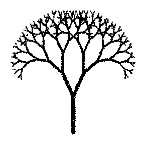
Fractal tree

ZZP

i-DDPM

Olympic rings

BPS

i-DDPM

Figure 1: Comparative results on two-dimensional generation of synthetic datasets.

In Table 1 we report the MMD score for five, $2$-dimensional toy distributions. We observe that the PDMP based generative models perform well compared to i-DDPM in all of these five datasets. In particular, ZZP and i-DDPM are implemented with the same neural network architecture, hence ZZP appears to compare favourably to i-DDPM with the same model expressivity. The results of Table 1 are supported by the plots of generated data shown in Figure 1, illustrating how ZZP and BPS are able to generate more detailed edges compared to i-DDPM. In Figure 2, we compare the output of RHMC and i-DDPM for a very small number of reverse steps. We observe how in this setting the data generated by RHMC are noticeably closer to the true data distribution compared to i-DDPM. This phenomenon is observed also for BPS as shown in Table 2, and is intuitively caused by the refreshment kernel, which is able to generate velocities that correct wrong positions. Respecting this intuition, ZZP does not perform as well as BPS and RHMC for a small number of reverse steps since its velocities are constrained to $\{-1,1\}$. Nonetheless, ZZP generates the most accurate results in our experiments given a large enough number of reverse steps. Additional results can be found in Appendix E, including some promising results applying the ZZP to the MNIST dataset.

steps	2	5	10	25	50	100	250
i-DDPM	696.28	192.17	45.08	12.34	11.78	8.72	11.71
BPS	165.09	22.18	5.48	1.58	3.01	3.66	2.07
RHMC	26.48	3.00	1.75	0.60	0.99	1.72	1.03
ZZP	358.25	89.49	11.31	1.20	0.71	1.04	0.42

Table 2: MMD $\downarrow$ on the 2D rose dataset, for the different methods at various number of backward steps, based on one run.

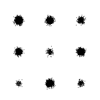
Gaussian grid

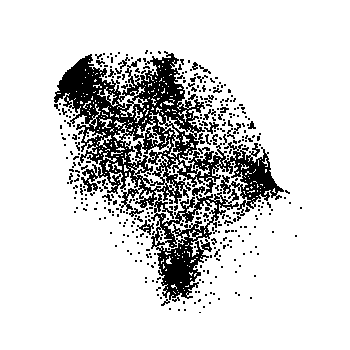
i-DDPM, 2 steps

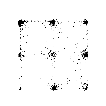
i-DDPM, 10 steps

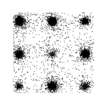
RHMC, 2 steps

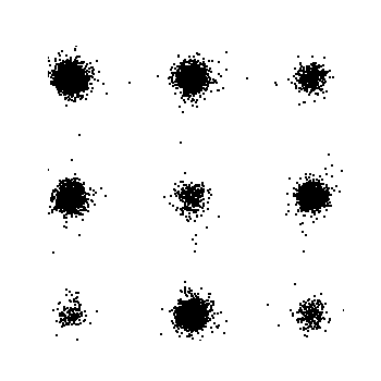
RHMC, 10 steps

Rose dataset

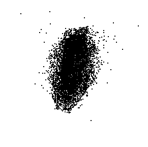
i-DDPM, 2 steps

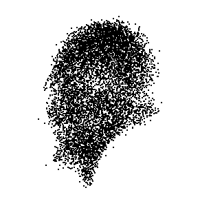
i-DDPM, 10 steps

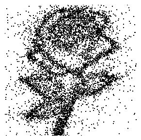
RHMC, 2 steps

RHMC, 10 steps

Figure 2: Comparing RHMC and i-DDPM for small number of reverse steps.

5 Discussion and conclusions

We have introduced new generative models based on piecewise deterministic Markov processes, developing a theoretically sound framework with specific focus on three PDMPs from the sampling literature. While this work lays the foundations of this class of methods, it also opens several directions worth investigating in the future.

Similarly to other generative models, our PDMP based algorithms are sensitive to the choice of the network architecture that is used to approximate the backward characteristics. Therefore, it is crucial to investigate which architectures are most suited for our algorithms in order to achieve state of the art performance in real world scenarios. For instance, in the case of BPS and RHMC it could be beneficial to separate the estimation of the density ratios and the generation of draws of the velocity conditioned on the position and time. For the case of ZZP, efficient techniques to learn the network in a high dimensional setting need to be investigated, while network architectures that resemble those used to approximate the score function appear to adapt well to the case of density ratios. Moreover, there are several alternative PDMPs that could be used as generative models and that we did not consider in detail in this paper, as for instance variance exploding alternatives.

Appendix

The Appendix is organised as follows. Appendix A includes the proofs and details regarding Section 2.1 and Section 2.2. Appendix B contains details and proofs regarding the framework of density ratio matching. Appendix C contains the pseudo-codes of the splitting schemes that are used to simulate the backward PDMPs. Appendix D contains the proof for Theorem 1 and some related details Finally, Appendix E contains the details on the numerical simulations, as well as additional results.

Appendix A PDMPs and their time reversals

A.1 Construction of a PDMP with multiple jump types

In this section we describe the formal construction of a non-homogeneous PDMP with the characteristics $(\Phi,\lambda,Q)$ where $\lambda,Q$ are of the form

$$\lambda(t,z)=\sum_{i=1}^{\ell}\lambda_{i}(t,z)\;,\quad Q(t,z,\mathrm{d}z^{\prime})=\sum_{i=1}^{\ell}\frac{\lambda_{i}(t,z)}{\lambda(t,z)}Q_{i}(t,z,\mathrm{d}z^{\prime})\;.$$ (14)

Recall the differential flow $\varphi:(t,s,z)\mapsto\varphi_{t,t+s}(z)$, which solves the ODE, $\mathrm{d}z_{t+s}=\Phi(t+s,z_{t+s})\mathrm{d}s$ for $s\geqslant 0$, i.e. $z_{t+s}=\varphi_{t,t+s}(z_{t})$. Similarly to the case of one type of jump only, we start the PDMP from an initial state $Z_{0}$, assume it is defined as $(Z_{t})_{t\in\left[0,\mathrm{T}_{n}\right]}$ on $\left[0,\mathrm{T}_{n}\right]$ for some $n\in\mathbb{N}$, and we now define define $(Z_{t})_{t\in\left[\mathrm{T}_{n},\mathrm{T}_{n+1}\right]}$. First, we define the proposals $(\tau^{i}_{n+1})_{i\in\{1,\ldots,\ell\}}$ for next event time as

$$\tau^{i}_{n+1}=\inf\left\{t>0:\int_{0}^{t}\lambda_{i}(T_{n}+u,\varphi_{\mathrm{T}_{n},\mathrm{T}_{n}+u}(Z_{\mathrm{T}_{n}}))\mathrm{d}u\geqslant E_{n+1}^{i}\right\}$$ (15)

where $E_{n+1}^{i}\sim\text{Exp}(1)$ for $i\in\{1,\ldots,\ell\}.$ Then define $i^{*}=\operatorname*{arg\,min}_{i\in\{1,\ldots,\ell\}}\tau^{i}_{n+1}$ and set the next jump time to

$$T_{n+1}=T_{n}+\tau^{i^{*}}_{n+1}.$$

The process is then defined on $\left[\mathrm{T}_{n},\mathrm{T}_{n+1}\right)$ by $Z_{\mathrm{T}_{n}+t}=\varphi_{\mathrm{T}_{n},\mathrm{T}_{n}+t}(Z_{\mathrm{T}_{n}})$ for $t\in[0,\tau_{n+1})$. Finally, we set $Z_{\mathrm{T}_{n+1}}\sim Q_{i^{*}}(T_{n+1},\varphi_{\mathrm{T}_{n},\mathrm{T}_{n}+\tau_{n+1}}(Z_{\mathrm{T}_{n}}),\cdot)$.

A.2 Extended generator

In order to define the generator of a PDMP, Davis [1993, Theorem 26.14] requires the set of conditions Davis [1993, (24.8)]. Notably, the PDMP is required to be non-explosive in the sense that the expected number of random events after any time $t$ starting the PDMP from any state should be finite. These conditions are verified for the forward PDMPs we consider.

H 3

The characteristics $(\Phi,\lambda,Q)$ satisfy the standard conditions [Davis, 1993, (24.8)].

Assuming H 3, Davis [1993, Theorem 26.14] gives that the extended generator of a PDMP with characteristics $(\Phi,\lambda,Q)$ is given by

$$\mathscr{L}_{t}f(z)=\langle\Phi(t,z),\nabla_{z}f(z)\rangle+\lambda(t,z)\int_{\mathbb{R}^{d}}(f(y)-f(z))Q(t,z,\mathrm{d}y)\;,$$ (16)

for all functions $f\in\mathrm{dom}(\mathscr{L}_{t})$, that is the space of measurable functions such that

$$M_{t}^{f}=f(Z_{t})-f(Z_{0})-\int_{0}^{t}\mathscr{L}_{s}f(Z_{s})\mathrm{d}s$$

is a local martingale. We also introduce the Carré du champ $\Gamma_{t}(f,g):=\mathscr{L}_{t}(fg)-f\mathscr{L}_{t}g-g\mathscr{L}_{t}f,$ with domain $\mathrm{dom}(\Gamma_{t}):=\{f,g:f,g,fg\in\mathrm{dom}(\mathscr{L}_{t})\}$ which in the case of a PDMP with generator (16) takes the form

$$\Gamma_{t}(f,g)(z)=\lambda(t,z)\int_{\mathbb{R}^{d}}(f(y)-f(z))(g(y)-g(z))Q(t,z,\mathrm{d}y)\;.$$ (17)

A.3 Proof of Proposition 1

In order to prove Proposition 1 we apply Conforti and Léonard [2022, Theorem 5.7] and hence in this section we verify the required assumptions. Before starting, we state the following technical condition which we omitted in Proposition 1 and is assumed in Conforti and Léonard [2022, Theorem 5.7].

H 4

It holds $\mathrm{C}_{c}^{2}(\mathbb{R}^{d})\subset\mathrm{dom}(\mathscr{L}_{t})$ for any $t\in\mathbb{R}_{+}$.

We now turn to verifying the remaining assumptions in Conforti and Léonard [2022, Theorem 5.7]. The “General Hypotheses” of Conforti and Léonard [2022] are satisfied since we assume the vector field $\Phi$ is locally bounded, the switching rate $(t,z)\mapsto\lambda(t,z)$ is a continuous function, and the jump kernel $Q$ is such that $Q(t,x,\cdot)$ is a probability distribution. In particular these assumptions imply that

$$\sup_{t\in[0,T],\lvert z\rvert\leqslant\rho}\int_{\mathbb{R}^{d}}(1\wedge\lvert z-y\rvert^{2})\lambda(t,z)Q(t,z,\mathrm{d}y)\leqslant\sup_{t\in[0,T],\lvert z\rvert\leqslant\rho}\lambda(t,z)<\infty\quad\text{for all }\rho\geqslant 0.$$ (18)

Then, Conforti and Léonard [2022, Theorem 5.7] requires a further integrability condition, which is satisfied when

$$\int_{[0,T]\times\mathbb{R}^{d}\times\mathbb{R}^{d}}(1\wedge\lvert z-y\rvert^{2})\mu_{0}P_{t}(\mathrm{d}z)\lambda(t,z)Q(t,z,\mathrm{d}y)<\infty.$$ (19)

It is then sufficient to have that

$$\int_{0}^{\mathrm{T}_{f}}\mathbb{E}[\lambda(t,Z_{t})]\mathrm{d}t<\infty$$ (20)

Finally, Conforti and Léonard [2022, Theorem 5.7] requires some technical assumptions which we now discuss. Introduce the class of functions that are twice continuously differentiable and compactly supported, denoted by $\mathcal{C}^{2}_{c}(\mathbb{R}^{d})$, and for $f\in\mathcal{C}^{2}_{c}(\mathbb{R}^{d})$ consider the two following conditions:

$$\int_{0}^{T}\int_{\mathbb{R}^{d}}\mu_{0}P_{t}(\mathrm{d}z)\lvert\mathscr{L}_{t}f(z)\rvert\mathrm{d}t<\infty,$$ (21)

$$\int_{0}^{T}\int_{\mathbb{R}^{d}}\mu_{0}P_{t}(\mathrm{d}z)\lvert\Gamma_{t}(f,g)(z)\rvert\mathrm{d}t<\infty\qquad\text{ for all }g\in\mathcal{C}^{2}_{c}(\mathsf{\mathbb{R}}^{d}).$$ (22)

We define $\mathcal{F}:=\{f\in\mathcal{C}^{2}_{c}(\mathsf{E}):\eqref{eq:integrab_generator},\eqref{eq:integrab_carreduchamp}\text{ hold }\}$. We need to verify that $\mathcal{F}\equiv\mathcal{C}^{2}_{c}(\mathsf{E}).$ Let us start by considering (21): we find

$$\int_{0}^{T}\mu_{0}P_{t}(\mathrm{d}z)\lvert\mathscr{L}_{t}f(z)\rvert\mathrm{d}t$$ (23)

$$\leqslant\int_{0}^{T}\mu_{0}P_{t}(\mathrm{d}z)\left(\lvert\langle\Phi(t,z),\nabla f(z)\rangle\rvert+\lambda(t,z)\int\lvert u(y)-u(z)\rvert Q(t,z,\mathrm{d}y)\right)\mathrm{d}t.$$ (24)

Since $f\in\mathcal{C}^{2}_{c}(\mathsf{E})$ we have that $\lvert\langle\Phi(t,z),\nabla f(z)\rangle\rvert$ is compactly supported and hence integrable, while the second term is finite assuming $\int_{0}^{T}\mathbb{E}[\lambda(t,Z_{t})]\mathrm{d}t<\infty.$ Under the latter assumption, (22) can be easily verified.

A.4 Proof of Proposition 2

Let us denote the initial condition of the forward PDMP by $\mu_{0}=\mu_{0}^{X}\otimes\mu_{0}^{V}$. First of all, notice that, for a PDMP with position-velocity decomposition and homogeneous jump kernel, the flux equation (3) becomes

$$\mu_{0}P_{\tilde{t}}(\mathrm{d}y,\mathrm{d}w)\overleftarrow{\lambda}(t,(y,w))\overleftarrow{Q}(t,(y,w),(\mathrm{d}x,\mathrm{d}v))=\mu_{0}P_{\tilde{t}}(\mathrm{d}x,\mathrm{d}v)\lambda(\tilde{t},(x,v))Q((x,v),(\mathrm{d}y,\mathrm{d}w))$$ (25)

where $\tilde{t}=\mathrm{T}_{f}-t.$ Moreover, since the jump kernel leaves the position vector unchanged we obtain that this is equivalent to

$$\mu_{0}P_{\tilde{t}}(\mathrm{d}w\rvert y)\overleftarrow{\lambda}(t,(y,w))\overleftarrow{Q}(t,(y,w),(\mathrm{d}x,\mathrm{d}v))=\mu_{0}P_{\tilde{t}}(\mathrm{d}v\rvert y)\lambda(\tilde{t},(y,v))Q((x,v),(\mathrm{d}y,\mathrm{d}w)),$$

where $\mu_{0}P_{t}(\mathrm{d}w\rvert y)$ is the conditional law of the velocity vector given the position vector at time $t$ with initial distribution $\mu_{0}.$

Suppose first that $Q((y,w),(\mathrm{d}x,\mathrm{d}v))=\updelta_{y}(\mathrm{d}x)\updelta_{\mathscr{R}_{y}w}(\mathrm{d}v)$ for an involution $\mathscr{R}_{y}$. Then we find

$$\mu_{0}P_{\tilde{t}}(\mathrm{d}w\rvert y)\overleftarrow{\lambda}(t,(y,w))\overleftarrow{Q}(t,(y,w),(\mathrm{d}x,\mathrm{d}v))=\mu_{0}P_{\tilde{t}}(\mathrm{d}\mathscr{R}_{y}w\rvert y)\lambda(\tilde{t},(y,\mathscr{R}_{y}w))\updelta_{y}(\mathrm{d}x)\updelta_{\mathscr{R}_{y}w}(\mathrm{d}v)$$

where we used that $\updelta_{\mathscr{R}_{y}w}(\mathrm{d}v)=\updelta_{\mathscr{R}_{y}v}(\mathrm{d}w)$ since $\mathscr{R}_{y}$ is an involution. Under our assumptions we have

$$\mu_{0}P_{\tilde{t}}(\mathrm{d}\mathscr{R}_{y}w\rvert y)=p_{\tilde{t}}(\mathscr{R}_{y}w\rvert y)\mu_{\mathrm{ref}}^{V}(\mathrm{d}w),\quad\mu_{0}P_{\tilde{t}}(\mathrm{d}w\rvert y)=p_{\tilde{t}}(w\rvert y)\mu_{\mathrm{ref}}^{V}(\mathrm{d}w),\;$$

since we assumed $\mu_{\mathrm{ref}}^{V}(\mathrm{d}w)=\mu_{\mathrm{ref}}^{V}(\mathrm{d}\mathscr{R}_{y}w).$ Hence we find for any $(y,w)\in\mathbb{R}^{2d}$ such that $p_{\tilde{t}}(w\rvert y)>0$

$$\overleftarrow{\lambda}(t,(y,w))\overleftarrow{Q}(t,(y,w),(\mathrm{d}x,\mathrm{d}v))=\frac{p_{\tilde{t}}(\mathscr{R}_{y}w\rvert y)}{p_{\tilde{t}}(w\rvert y)}\lambda(\tilde{t},(y,\mathscr{R}_{y}w))\updelta_{y}(\mathrm{d}x)\updelta_{\mathscr{R}_{y}w}(\mathrm{d}v).$$

This can only be satisfied if

$$\overleftarrow{\lambda}(t,(y,w))=\frac{p_{\tilde{t}}(\mathscr{R}_{y}w\rvert y)}{p_{\tilde{t}}(w\rvert y)}\lambda(\tilde{t},(y,\mathscr{R}_{y}w)),\quad Q(t,(y,w),(\mathrm{d}x,\mathrm{d}v))=\updelta_{y}(\mathrm{d}x)\updelta_{\mathscr{R}_{y}w}(\mathrm{d}v).$$

Consider now the second case, that is $Q((y,w),(\mathrm{d}x,\mathrm{d}v))=\updelta_{y}(\mathrm{d}x)\nu(\mathrm{d}v\rvert y)$ and $\lambda(t,(y,w))=\lambda(t,y)$. The flux equation (3) can be rewritten as

$$\mu_{0}P_{\tilde{t}}(\mathrm{d}w\rvert y)\overleftarrow{\lambda}(t,(y,w))\overleftarrow{Q}(t,(y,w),(\mathrm{d}x,\mathrm{d}v))=\mu_{0}P_{\tilde{t}}(\mathrm{d}v\rvert y)\lambda(\tilde{t},y)\updelta_{y}(\mathrm{d}x)\nu(\mathrm{d}w\rvert y)$$

Under our assumptions we have $\nu(\mathrm{d}w\rvert y)=(\mathrm{d}\nu/\mathrm{d}\mu_{\mathrm{ref}}^{V})(w\rvert y)\mu_{\mathrm{ref}}^{V}(\mathrm{d}w)$ and $\mu_{0}P_{\tilde{t}}(\mathrm{d}w\rvert y)=p_{\tilde{t}}(w\rvert y)\mu_{\mathrm{ref}}^{V}(\mathrm{d}w)$ for some measure $\mu_{\mathrm{ref}}^{V}$. Hence for any $(y,w)\in\mathbb{R}^{2d}$ such that $p_{\tilde{t}}(w\rvert y)>0$ we obtain

$$\overleftarrow{\lambda}(t,(y,w))\overleftarrow{Q}(t,(y,w),(\mathrm{d}x,\mathrm{d}v))=\frac{(\mathrm{d}\nu/\mathrm{d}\mu_{\mathrm{ref}}^{V})(w\rvert y)}{p_{\tilde{t}}(w\rvert y)}\lambda(\tilde{t},y)p_{\tilde{t}}(\mathrm{d}v\rvert y)\updelta_{y}(\mathrm{d}x).\;$$ (26)

This is satisfied when

$$\overleftarrow{\lambda}(t,(y,w))=\frac{(\mathrm{d}\nu/\mathrm{d}\mu_{\mathrm{ref}}^{V})(w\rvert y)}{p_{\tilde{t}}(w\rvert y)}\lambda(\tilde{t},y),\quad\overleftarrow{Q}(t,(y,w),(\mathrm{d}x,\mathrm{d}v))=\mu_{0}P_{\tilde{t}}(\mathrm{d}v\rvert y)\updelta_{y}(\mathrm{d}x).$$

A.5 Extension of Proposition 2 to multiple jump types

Proposition 2 considers PDMPs with one type of jump, while here we discuss the case of characteristics of the form (14), which is e.g. the case of ZZP and BPS. In this setting we can assume the backward jump rate and kernel have a similar structure, that is

$$\overleftarrow{\lambda}(t,z)=\sum_{i=1}^{\ell}\overleftarrow{\lambda}_{i}(t,z)\;,\quad\overleftarrow{Q}(t,z,\mathrm{d}z^{\prime})=\sum_{i=1}^{\ell}\frac{\overleftarrow{\lambda}_{i}(t,z)}{\overleftarrow{\lambda}(t,z)}\overleftarrow{Q}_{i}(t,z,\mathrm{d}z^{\prime})\;,$$ (27)

in which case the balance condition (3) can be rewritten as

$$\mu_{0}P_{\mathrm{T}_{f}-t}(\mathrm{d}y)\sum_{i=1}^{\ell}\overleftarrow{\lambda}_{i}(t,y)\overleftarrow{Q}_{i}(t,y,\mathrm{d}z)=\mu_{0}P_{\mathrm{T}_{f}-t}(\mathrm{d}z)\sum_{i=1}^{\ell}\lambda_{i}(\mathrm{T}_{f}-t,z)Q_{i}(\mathrm{T}_{f}-t,z,\mathrm{d}y)\;.$$ (28)

It is then enough that

$$\mu_{0}P_{\mathrm{T}_{f}-t}(\mathrm{d}y)\overleftarrow{\lambda}_{i}(t,y)\overleftarrow{Q}_{i}(t,y,\mathrm{d}z)=\mu_{0}P_{\mathrm{T}_{f}-t}(\mathrm{d}z)\lambda_{i}(\mathrm{T}_{f}-t,z)Q_{i}(\mathrm{T}_{f}-t,z,\mathrm{d}y)\;$$ (29)

holds for all $i\in\{1,\dots,\ell\}.$ It follows that it is sufficient to apply Proposition 2 to each pair $(\lambda_{i},Q_{i})$ to obtain $(\overleftarrow{\lambda}_{i},\overleftarrow{Q}_{i})$ such that (3) holds.

A.6 Time reversals of ZZP, BPS, and RHMC

In this section we give rigorous statements regarding time reversals of ZZP, BPS, and RHMC. For all samplers we rely on Proposition 2 and hence we focus on verifying its assumptions. In the cases of ZZP and RHMC we assume the technical condition H 4 since proving it rigorously is out of the scope of the present paper. We remark that this can be proved with techniques as in Durmus et al. [2021], which show H 4 in the case of BPS.

Proposition 4 (Time reversal of ZZP)

Consider a ZZP $(X_{t},V_{t})_{t\in[0,\mathrm{T}_{f}]}$ with initial distribution $\mu_{\star}\otimes\nu$, where $\nu=\mathrm{Unif}(\{\pm 1\}^{d})$ and invariant distribution $\pi\otimes\nu$, where $\pi$ has potential $\psi$ satisfying H 1. Assume that H 4 holds and that $\int\mu_{\star}(\mathrm{d}x)\lvert\partial_{i}\psi(x)\rvert<\infty$ for all $i=1,\dots,d.$ Then the time reversal of the ZZP has vector field

$$\overleftarrow{\Phi}^{\mathrm{Z}}(x,v)=(-v,0)^{T}$$

and jump rates and kernels are given for all $(y,w)\in\mathbb{R}^{2d}$ such that $P_{\mathrm{T}_{f}-t}(w\rvert y)>0$ by

$$\overleftarrow{\lambda}_{i}^{\mathrm{Z}}(t,(y,w))=\frac{p_{\mathrm{T}_{f}-t}(\mathscr{R}_{i}^{\mathrm{Z}}w\rvert y)}{p_{\mathrm{T}_{f}-t}(w\rvert y)}\lambda^{\mathrm{Z}}_{i}(y,\mathscr{R}_{i}^{\mathrm{Z}}w),\quad\overleftarrow{Q}_{i}^{\mathrm{Z}}((y,w),(\mathrm{d}x,v))=\updelta_{(y,\mathscr{R}^{\mathrm{Z}}_{i}w)}(\mathrm{d}x,v)$$ (30)

for $i=1,\dots,d$.

Proof

We verify the conditions of Proposition 2 corresponding to deterministic transitions and rely on Section A.5 to apply the proposition to each pair $(\lambda^{\mathrm{Z}}_{i},Q^{\mathrm{Z}}_{i})$. First notice the vector field $\Phi(x,v)=(v,0)^{T}$ is clearly locally bounded and $(t,x)\mapsto\lambda(x,v)$ is continuous since $\psi$ is continuously differentiable. Moreover, the ZZP can be shown to be non-explosive applying Durmus et al. [2021, Proposition 9]. Then, we need to verify (20). First, observe that $\mathbb{E}[\lambda_{i}(X_{t},V_{t})]\leqslant\mathbb{E}[\lvert\partial_{i}\psi(X_{t})\rvert].$ Then

$$\mathbb{E}[\lvert\partial_{i}\psi(X_{t})\rvert] =\mathbb{E}\left[\left\lvert\partial_{i}\psi(X_{0})+\int_{0}^{1}\langle X_{t}-X_{0},\nabla\partial_{i}\psi(X_{0}+s(X_{t}-X_{0}))\rangle\mathrm{d}s\right\rvert\right]$$ (31)

$$\leqslant\mathbb{E}[\lvert\partial_{i}\psi(X_{0})\rvert]+\mathbb{E}\left[\int_{0}^{1}\lvert\langle X_{t}-X_{0},\nabla^{2}\psi(X_{0}+s(X_{t}-X_{0}))\mathsf{e}_{i}\rangle\rvert\mathrm{d}s\right]$$ (32)

where $\mathsf{e}_{i}$ is the $i$-th vector of the canonical basis. Notice that $\lvert X_{t}-X_{0}\rvert\leqslant t\sqrt{d}$. Thus we find

$$\mathbb{E}[\lvert\partial_{i}\psi(X_{t})\rvert] \leqslant\mathbb{E}[\lvert\partial_{i}\psi(X_{0})\rvert]+t\sqrt{d}\sup_{x\in\mathbb{R}^{d}}\lVert\nabla^{2}\psi(x)\rVert$$ (33)

and therefore

$$\int_{0}^{\mathrm{T}_{f}}\mathbb{E}[\lambda(X_{t},V_{t})]\mathrm{d}t\leqslant\mathrm{T}_{f}\sum_{i=1}^{d}\left(\mathbb{E}\lvert\partial_{i}\psi(X_{0})\rvert+\frac{\mathrm{T}_{f}}{2}\sqrt{d}\sup_{x\in\mathbb{R}^{d}}\lVert\nabla^{2}\psi(x)\rVert\right).$$ (34)

Since $\mathbb{E}_{\mu_{\star}}\lvert\partial_{i}\psi(X)\rvert<\infty$ and because we are assuming H 1, we obtain (20). Finally, notice that $P_{t}(\mathrm{d}v\rvert x)$ is absolutely continuous with respect to the counting measure on $\{1,-1\}^{d}$, which is clearly invariant with respect to $\mathscr{R}^{\mathrm{Z}}_{i}$. $\square$

Proposition 5 (Time reversal of BPS)

Consider a BPS $(X_{t},V_{t})_{t\in[0,\mathrm{T}_{f}]}$ with initial distribution $\mu_{\star}\otimes\nu$, where $\nu=\mathrm{Unif}(\mathsf{S}^{d-1})$, and invariant distribution $\pi\otimes\nu$, where $\pi$ has potential $\psi$ satisfying H 1. Assume that $\mathbb{E}_{\mu_{\star}}[|\nabla\psi(X)\rvert]<\infty.$ Then there exists a density $p_{t}(w\rvert y):=\nicefrac{{\mathrm{d}(\mu_{0}P_{t})(\mathrm{d}w\rvert y)}}{{\nu(\mathrm{d}w)}}.$ Moreover, the time reversal of the BPS has vector field

$$\overleftarrow{\Phi}^{\mathrm{B}}(x,v)=(-v,0)^{T},$$

while the jump rates and kernels are given for all $t,y,w\in[0,\mathrm{T}_{f}]\times\mathbb{R}^{2d}$ such that $p_{\mathrm{T}_{f}-t}(w\rvert y)>0$ by

$$\overleftarrow{\lambda}_{1}^{\mathrm{B}}(t,(y,w))=\frac{p_{\tilde{t}}(\mathscr{R}^{\mathrm{B}}_{y}w\rvert y)}{p_{\tilde{t}}(w\rvert y)}\lambda_{1}^{\mathrm{B}}(y,\mathscr{R}^{\mathrm{B}}_{y}w),\,\,\overleftarrow{Q}_{1}^{\mathrm{B}}((y,w),(\mathrm{d}x,\mathrm{d}v))=\updelta_{(y,\mathscr{R}^{\mathrm{B}}_{y}w)}(\mathrm{d}x,\mathrm{d}v),$$ (35)

$$\overleftarrow{\lambda}_{2}^{\mathrm{B}}(t,(y,w))=\lambda_{r}\frac{1}{p_{\mathrm{T}_{f}-t}(w|y)},\quad\overleftarrow{Q}_{2}^{\mathrm{B}}(t,(y,w),(\mathrm{d}x,\mathrm{d}v))=\mu_{0}P_{\mathrm{T}_{f}-t}(\mathrm{d}v\rvert y)\updelta_{y}(\mathrm{d}x)\mathrm{d}v,$$ (36)

where $\tilde{t}=\mathrm{T}_{f}-t$.

Remark 3

Under the assumption that $\nu$ is the uniform distribution on the sphere, it is natural to take $\mu_{\mathrm{ref}}^{\mathrm{V}}=\nu$, which gives that $\nicefrac{{\mathrm{d}\nu}}{{\mathrm{d}\mu_{\mathrm{ref}}^{V}}}=1$ and hence the backward refreshment rate is as in (36). When $\nu$ is the $d$-dimensional Gaussian distribution, the natural choice is to let $\mu_{\mathrm{ref}}^{\mathrm{V}}$ be the Lebesgue measure and hence we obtain a rate as given in (5).

Proof

We verify the general conditions of Proposition 2, then focusing on the deterministic jumps and the refreshments relying on Section A.5. The BPS was shown to be non-explosive for any initial distribution in Durmus et al. [2021, Proposition 10]. Since $\lambda(t,(x,v))=\lambda(x,v)=\langle v,\nabla\psi(x)\rangle_{+}$, with a similar reasoning of the proof of Proposition 4 we have

$$\mathbb{E}[\lambda(X_{t},V_{t})]=\mathbb{E}\left[\left(\langle V_{t},\nabla\psi(X_{0})\rangle+\int_{0}^{1}\langle V_{t},\nabla^{2}\psi(X_{0}+s(X_{t}-X_{0}))(X_{t}-X_{0})\rangle\mathrm{d}s\right)_{+}\right].$$ (37)

Taking advantage of $\lvert V_{t}\rvert=1$ we have $\lvert X_{t}-X_{0}\rvert\leqslant t$ and thus we find

$$\mathbb{E}[\lambda(X_{t},V_{t})] \leqslant\mathbb{E}\left[|\nabla\psi(X_{0})\rvert+\int_{0}^{1}\lvert\nabla^{2}\psi(X_{0}+s(X_{t}-X_{0}))(X_{t}-X_{0})\rvert\mathrm{d}s\right]$$ (38)

$$\leqslant\mathbb{E}\left[|\nabla\psi(X_{0})\rvert\right]+t\sup_{x\in\mathbb{R}^{d}}\lVert\nabla^{2}\psi(x)\rVert.$$ (39)

This is sufficient to obtain (20) since $\mathbb{E}[|\nabla\psi(X_{0})\rvert]<\infty$ and we assume H 1. Moreover, H 4 holds by Durmus et al. [2021, Proposition 23]. Finally notice that $P_{t}(\mathrm{d}v\rvert x)$ is absolutely continuous with respect to $\mu_{\mathrm{ref}}^{\mathrm{V}}=\mathrm{Unif}(\mathsf{S}^{d-1})$, which satisfies $\mu_{\mathrm{ref}}^{\mathrm{B}}(\mathscr{R}^{\mathrm{B}}(x)v)=\mu_{\mathrm{ref}}^{\mathrm{B}}(v)$ for all $x,v\in\mathbb{R}^{d}\times\mathsf{S}^{d-1}$. All the required assumptions in Proposition 2 are thus satisfied. $\square$

Proposition 6 (Time reversal of RHMC)

Consider a RHMC $(X_{t},V_{t})_{t\in[0,\mathrm{T}_{f}]}$ with initial distribution $\mu_{\star}\otimes\nu$, where $\nu$ is the $d$-dimensional standard normal distribution, and invariant distribution $\pi\otimes\nu$, where $\pi$ has potential $\psi\in\mathcal{C}^{1}(\mathbb{R}^{d})$. Suppose that H 4 holds and that for any $y\in\mathbb{R}^{d}$, $P_{t}(\mathrm{d}w|y)$ is absolutely continuous with respect to Lebesgue measure, with density $p_{t}(w\rvert y)$. Then the time reversal of the RHMC has vector field

$$\overleftarrow{\Phi}^{\mathrm{H}}(x,v)=(-v,\nabla\psi(x))^{T},$$

while the jump rates and kernels are given for all $(y,w)\in\mathbb{R}^{2d}$ such that $p_{\mathrm{T}_{f}-t}(w\rvert y)>0$ by

$$\overleftarrow{\lambda}_{2}^{\mathrm{H}}(t,(y,w))=\lambda_{r}\frac{\nu(w)}{p_{\mathrm{T}_{f}-t}(w|y)},\quad\overleftarrow{Q}_{2}^{\mathrm{H}}(t,(y,w),(\mathrm{d}x,\mathrm{d}v))=p_{\mathrm{T}_{f}-t}(v\rvert y)\updelta_{y}(\mathrm{d}x)\mathrm{d}v.$$ (40)

Proof

First of all, RHMC is non-explosive by Durmus et al. [2021, Proposition 8]. Then $\Phi$ is locally bounded and (20) is trivially satisfied. Finally, we can take $\mu_{\mathrm{ref}}^{\mathrm{V}}$ to be the Lebesgue measure. $\square$

Appendix B Density ratio matching

B.1 Ratio matching with Bregman divergences

We now describe a general approach to approximate ratios of densities based on the minimisation of Bregman divergences [Sugiyama et al., 2011], which as we discuss is closely connected to the loss of Hyvärinen [2007].

For a differentiable, strictly convex function $f$ we define the Bregman divergence $\mathrm{B}_{f}(r,s):=f(r)-f(s)-f^{\prime}(s)(r-s)$. Given two time-dependent probability density functions on $\mathbb{R}^{2d}$, $p,q$, we wish to approximate their ratio $r(x,v,t)=\nicefrac{{p_{t}(x,v)}}{{q_{t}(x,v)}}$ for $t\in[0,\mathrm{T}_{f}]$ with a parametric function $s_{\theta}:\mathbb{R}^{d}\times\mathbb{R}^{d}\times[0,\mathrm{T}_{f}]\to\mathbb{R}_{+}$ by solving the minimisation problem

$$\min_{\theta}\int_{0}^{\mathrm{T}_{f}}\omega(t)\,\mathbb{E}\Big{[}\mathrm{B}_{f}(r(X_{t},V_{t},t),s_{\theta}(X_{t},V_{t},t))\Big{]}\mathrm{d}t,$$ (41)

where the expectation is with respect to the joint density $q_{t}(x,v)$, that is $(X_{t},V_{t})\sim q_{t}$, while $\omega$ is a probability density function for the time variable. Well studied choices of the function $f$ include e.g. $f(r)=r\log r-r$, that is related to a KL divergence, or $f(r)=(r-1)^{2}$, related to the square loss, or $f(r)=r\log r-(1+r)\log(1+r),$ which corresponding to solving a logistic regression task. Ignoring terms that do not depend on $\theta$ we can rewrite the minimisation as

$$\min_{\theta}\int_{0}^{\mathrm{T}_{f}}\!\!\!\omega(t)\left(\mathbb{E}_{p_{t}}\big{[}f^{\prime}(s_{\theta}(X_{t},V_{t},t))s_{\theta}(X_{t},V_{t},t)-f(s_{\theta}(X_{t},V_{t},t))\big{]}-\mathbb{E}_{q_{t}}\big{[}f^{\prime}(s_{\theta}(X_{t},V_{t},t))\big{]}\right)\mathrm{d}t.$$ (42)

Notably this is independent of the true density ratio and thus it is a formulation with similar spirit to implicit score matching. Naturally, in practice the loss can be approximated empirically with a Monte Carlo average.

B.2 Details and proofs regarding Hyvärinen’s ratio matching

B.2.1 Connection to Bregman divergences

In the next statement, we show that the loss ${\ell}_{\mathrm{I}}$ defined in (6), or equivalently its explicit counterpart ${\ell}_{\mathrm{E}}$ (see Proposition 3), can be put in the framework of Bregman divergences.

Corollary 1

Recall $\mathbf{G}(r)=(1+r)^{-1}$ and let $f(r)=\nicefrac{{(r-1)^{2}}}{{2}}.$ The task $\min_{\theta}{\ell}_{\mathrm{E}}(\theta)$ is equivalent to

$$\min_{\theta} \sum_{i=1}^{d}\;\mathbb{E}_{p_{t}}\Big{[}\mathrm{B}_{f}(\mathbf{G}(s_{i}^{\theta}(X_{t},V_{t},t)),\mathbf{G}(r_{i}(X_{t},V_{t},t)))$$ (43)

$$\quad+\mathrm{B}_{f}(\mathbf{G}(s_{i}^{\theta}(X_{t},\mathscr{R}_{i}^{\mathrm{Z}}V_{t},t)),\mathbf{G}(r_{i}(X_{t},\mathscr{R}_{i}^{\mathrm{Z}}V_{t},t)))\Big{]}$$ (44)

Proof

The result follows by straightforward computations. $\square$

B.2.2 Proof of Proposition 3

The proof follows the same lines as Hyvärinen [2007, Theorem 1]. We find

$${\ell}_{\mathrm{E}}(\theta) =C+\int_{0}^{\mathrm{T}_{f}}\omega(t)\sum_{i=1}^{d}\mathbb{E}_{p_{t}}\Big{[}\mathbf{G}^{2}(s_{i}^{\theta}(X_{t},V_{t},t))+\mathbf{G}^{2}(s_{i}^{\theta}(X_{t},\mathscr{R}_{i}^{\mathrm{Z}}V_{t},t))$$ (45)

$$\quad-2\mathbf{G}(r_{i}(X_{t},V_{t},t))\mathbf{G}(s_{i}^{\theta}(X_{t},V_{t},t))-2\mathbf{G}(s_{i}^{\theta}(X_{t},\mathscr{R}_{i}^{\mathrm{Z}}V_{t},t))\mathbf{G}(r_{i}(X_{t},\mathscr{R}_{i}^{\mathrm{Z}}V_{t},t))\Big{]}\mathrm{d}t,$$ (46)

where $C$ is a constant independent of $\theta.$ Then plugging in the expression of $\mathbf{G}$ we can rewrite the last term as

$$\mathbb{E}_{p_{t}}\Big{[}\mathbf{G}(s_{i}^{\theta}(X_{t},\mathscr{R}_{i}^{\mathrm{Z}}V_{t},t))\mathbf{G}(r_{i}(X_{t},\mathscr{R}_{i}^{\mathrm{Z}}V_{t},t))\Big{]}$$ (47)

$$=\int\sum_{v\in\{\pm 1\}^{d}}p_{t}(x,v)\mathbf{G}(s_{i}^{\theta}(x,\mathscr{R}_{i}^{\mathrm{Z}}v,t))\frac{p_{t}(x,\mathscr{R}_{i}^{\mathrm{Z}}v)}{p_{t}(x,v)+p_{t}(x,\mathscr{R}_{i}^{\mathrm{Z}}v)}\mathrm{d}x$$ (48)

$$=\mathbb{E}_{p_{t}}\Big{[}\mathbf{G}(s_{i}^{\theta}(X_{t},V_{t},t))\frac{p_{t}(X_{t},\mathscr{R}_{i}^{\mathrm{Z}}V_{t})}{p_{t}(X_{t},V_{t})+p_{t}(X_{t},\mathscr{R}_{i}^{\mathrm{Z}}V_{t})}\Big{]}.$$ (49)

Therefore we find

$${\ell}_{\mathrm{E}}(\theta)=C+\int_{0}^{\mathrm{T}_{f}}\omega(t)\sum_{i=1}^{d}\mathbb{E}_{p_{t}}\Bigg{[}\mathbf{G}^{2}(s_{i}^{\theta}(X_{t},V_{t},t))+\mathbf{G}^{2}(s_{i}^{\theta}(X_{t},\mathscr{R}_{i}^{\mathrm{Z}}V_{t},t))$$ (50)

$$\quad-\frac{2\mathbf{G}(s_{i}^{\theta}(X_{t},V_{t},t))\,p_{t}(X_{t},V_{t})}{p_{t}(X_{t},V_{t})+p_{t}(X_{t},\mathscr{R}_{i}^{\mathrm{Z}}V_{t})}-\frac{2\mathbf{G}(s_{i}^{\theta}(X_{t},V_{t},t))\,p_{t}(X_{t},\mathscr{R}_{i}^{\mathrm{Z}}V_{t})}{p_{t}(X_{t},V_{t})+p_{t}(X_{t},\mathscr{R}_{i}^{\mathrm{Z}}V_{t})}\Bigg{]}\mathrm{d}t$$ (51)

$$=C+\!\int_{0}^{\mathrm{T}_{f}}\!\!\!\omega(t)\sum_{i=1}^{d}\mathbb{E}_{p_{t}}\Big{[}\mathbf{G}^{2}(s_{i}^{\theta}(X_{t},V_{t},t))+\mathbf{G}^{2}(s_{i}^{\theta}(X_{t},\mathscr{R}_{i}^{\mathrm{Z}}V_{t},t))-2\mathbf{G}(s_{i}^{\theta}(X_{t},V_{t},t))\Big{]}\mathrm{d}t.$$ (52)

Appendix C Discretisations of time reversed PDMPs with splitting schemes

Here we discuss the splitting schemes we use to discretise the backward PDMPs. We give the pseudo-code for RHMC in Algorithm 1, and discuss the cases of ZZP and BPS below. For further details on this class of approximations we refer the reader to Bertazzi et al. [2023].

Initialise either from $(\overline{X}_{0},\overline{V}_{0})\sim\pi\otimes\nu$ or $(\overline{X}_{0},\overline{V}_{0})\sim\pi(\mathrm{d}x)p_{\theta^{*}}(\mathrm{d}v\rvert x,\mathrm{T}_{f})$;

for $n=0,\dots,N-1$ do

       $(\widetilde{X},\widetilde{V})=\varphi^{\mathrm{H}}_{-\nicefrac{{\delta_{n+1}}}{{2}}}(\overline{X}_{t_{n}},\overline{V}_{t_{n}})$ ;

       $\widetilde{t}=\mathrm{T}_{f}-t_{n}-\frac{\delta_{n+1}}{2}$ ;

       Estimate ratio: $\overline{s}=\nicefrac{{\nu(\widetilde{V})}}{{p_{\theta^{*}}(\;\widetilde{V}\rvert\;\widetilde{X},\;\widetilde{t}\;)}}$ ;

       Draw proposal $\tau_{n+1}\sim\mathrm{Exp}(\overline{s}\lambda_{r})$ ;

       if $\tau_{n+1}\leqslant\delta_{n+1}$ then

             Draw $\widetilde{V}\sim p_{\theta^{*}}(\,\cdot\,\rvert\widetilde{X},\;\widetilde{t}\;)$;

            

       end if

      $(\overline{X}_{t_{n+1}},\overline{V}_{t_{n+1}})=\varphi^{\mathrm{H}}_{-\nicefrac{{\delta_{n+1}}}{{2}}}(\widetilde{X},\widetilde{V})$;

      

end for

Algorithm 1 Splitting scheme DJD for the time reversed RHMC

Initialise $(\overline{X}_{0},\overline{V}_{0})\sim\pi\otimes\nu$;

for $n=0,\dots,N-1$ do

       $\widetilde{X}=\overline{X}_{t_{n}}-\frac{\delta_{n+1}}{2}\;\overline{V}_{t_{n}}$ ;

       $\widetilde{V}=\overline{V}_{t_{n}}$ ;

       $\widetilde{t}=\mathrm{T}_{f}-t_{n}-\frac{\delta_{n+1}}{2}$ ;

       Estimate density ratios: $s^{\theta^{*}}(\widetilde{X},\widetilde{V},\widetilde{t}\;)$ ;

       for $i=1\dots,d$ do

             With probability $(1-\exp(-\delta_{n+1}\;s^{\theta^{*}}_{i}(\widetilde{X},\widetilde{V},\widetilde{t}\;)\;\lambda_{i}(\widetilde{X},\mathscr{R}^{\mathrm{Z}}_{i}\widetilde{V})))$ set $\widetilde{V}=\mathscr{R}_{i}^{\mathrm{Z}}\widetilde{V}$ ;

            

       end for

      $\overline{X}_{t_{n+1}}=\widetilde{X}-\frac{\delta_{n+1}}{2}\;\widetilde{V}$ ;

       $\overline{V}_{t_{n+1}}=\widetilde{V}$ ;

      

end for

Algorithm 2 Splitting scheme DJD for the time reversed ZZP

Initialise either from $(\overline{X}_{0},\overline{V}_{0})\sim\pi\otimes\nu$ or $(\overline{X}_{0},\overline{V}_{0})\sim\pi(\mathrm{d}x)p_{\theta^{*}}(\;\cdot\;\rvert x,\mathrm{T}_{f})$ ;

for $n=0,\dots,N-1$ do

       $\widetilde{V}=\overline{V}_{t_{n}}$ ;

       Estimate density ratio: $\overline{s}_{2}=\nicefrac{{\nu(\widetilde{V})}}{{p_{\theta^{*}}(\;\widetilde{V}\rvert\;\overline{X}_{t_{n}},\;\mathrm{T}_{f}-t_{n})}}$ ;

       With probability $(1-\exp(-\lambda_{r}\overline{s}_{2}\;\frac{\delta_{n+1}}{2}))$ draw $\widetilde{V}\sim p_{\theta^{*}}(\;\cdot\;\rvert\overline{X}_{t_{n}},\mathrm{T}_{f}-t_{n})$ ;

       $\widetilde{X}=\overline{X}_{t_{n}}-\frac{\delta_{n+1}}{2}\;\overline{V}_{t_{n}}$ ;

       $\widetilde{t}=\mathrm{T}_{f}-t_{n}-\frac{\delta_{n+1}}{2}$ ;

       Estimate density ratio: $\overline{s}_{1}=\nicefrac{{p_{\theta^{*}}(\mathscr{R}^{\mathrm{B}}_{\widetilde{X}}\widetilde{V}\rvert\;\widetilde{X},\;\widetilde{t}\;)}}{{p_{\theta^{*}}(\;\widetilde{V}\rvert\;\widetilde{X},\;\widetilde{t}\;)}}$ ;

       With probability $(1-\exp(-\delta_{n+1}\overline{s}_{1}\lambda_{1}(\widetilde{X},\mathscr{R}^{\mathrm{B}}_{\widetilde{X}}\widetilde{V})))$ set $\widetilde{V}=\mathscr{R}^{\mathrm{B}}_{\widetilde{X}}\widetilde{V}$ ;

       $\overline{X}_{t_{n+1}}=\widetilde{X}-\frac{\delta_{n+1}}{2}\;\widetilde{V}$ ;

       Estimate density ratio: $\overline{s}_{2}=\nicefrac{{\nu(\widetilde{V})}}{{p_{\theta^{*}}(\;\widetilde{V}\rvert\;\overline{X}_{t_{n+1}},\;\mathrm{T}_{f}-t_{n+1})}}$ ;

       With probability $(1-\exp(-\lambda_{r}\overline{s}_{2}\;\frac{\delta_{n+1}}{2}))$ draw $\widetilde{V}\sim p_{\theta^{*}}(\;\cdot\;\rvert\overline{X}_{t_{n}},\mathrm{T}_{f}-t_{n+1})$ ;

       $\overline{V}_{t_{n+1}}=\widetilde{V}$ ;

      

end for

Algorithm 3 Splitting scheme RDBDR for the time reversed BPS

C.1 Simulating the backward ZZP

For ZZP we apply the splitting scheme DJD discussed in Section 2.4, with the only difference that we allow multiple velocity flips during the jump step similarly to Bertazzi et al. [2023]. Algorithm 2 gives a pseudo-code.

C.2 Simulating the backward BPS

In the case of BPS, we follow the recommendations of Bertazzi et al. [2023] and adapt their splitting scheme RDBDR, where R stands for refreshments, D for deterministic motion, and B for bounces. We give a pseudo-code in Algorithm 3. We remark that an alternative is to use the scheme DJD for BPS, simulating reflections and refreshments in the J part of the splitting. This choice has the advantage of reducing the number of model evaluations.

Appendix D Discussion and proof for Theorem 1

D.1 Discussion on H 2

In this section we discuss H 2 in the case of ZZP, BPS, and RHMC. For all three of these samplers, existing theory shows convergence of the form

$$\lVert\updelta_{(x,v)}P_{t}-\pi\otimes\nu\rVert_{V}\leqslant C^{\prime}e^{-\gamma t}V(x,v),$$ (53)

where $V:\mathbb{R}^{2d}\to[1,\infty)$ is a positive function and $\lVert\mu\rVert_{V}:=\sup_{\lvert g\rvert\leqslant V}\lvert\mu(g)\rvert$ is the $V$-norm. When the initial condition of the process is $\mu_{\star}\otimes\nu$, we obtain the bound

$$\lVert\mu_{\star}\otimes\nu P_{t}-\pi\otimes\nu\rVert_{V}\leqslant C^{\prime}e^{-\gamma t}\mu_{\star}\otimes\nu(V),$$ (54)

which translates to a bound in TV distance, since we assume $V\geqslant 1$. Conditions on $\pi$ ensuring (53) can be found for ZZP in Bierkens et al. [2019b], for BPS in Deligiannidis et al. [2019], Durmus et al. [2020], and for RHMC in Bou-Rabee and Sanz-Serna [2017]. Observe that we can set the constant $C$ in H 2 to $C=C^{\prime}\mu_{\star}\otimes\nu(V)$. Clearly, $C$ is finite whenever $\mu_{\star}\otimes\nu(V)<\infty.$ Since $V$ is such that $\lim_{\lvert z\rvert\to\infty}V(z)=+\infty$, showing $C$ is finite requires suitable tail conditions on the initial distribution $\mu_{\star}\otimes\nu.$

D.2 Proof of Theorem 1

First notice that

$$\lVert\mu_{\star}-\mathcal{L}(\overline{X}_{\mathrm{T}_{f}})\rVert_{\mathrm{TV}}\leqslant\lVert\mu_{\star}\otimes\nu-\mathcal{L}(\overline{X}_{\mathrm{T}_{f}},\overline{V}_{\mathrm{T}_{f}})\rVert_{\mathrm{TV}}\;,$$ (55)

hence we focus on bounding the right hand side. Under our assumptions, the forward PDMP $(X_{t},V_{t})_{t\in[0,\mathrm{T}_{f}]}$ admits a time reversal that is a PDMP $(\overleftarrow{X}_{t},\overleftarrow{V}_{t})_{t\in[0,\mathrm{T}_{f}]}$ with characteristics $(\overleftarrow{\Phi},\overleftarrow{\lambda},\overleftarrow{Q})$ satisfying the conditions in Proposition 1. Therefore, it holds $\mu_{\star}\otimes\nu=\mathcal{L}(\overleftarrow{X}_{\mathrm{T}_{f}},\overleftarrow{V}_{\mathrm{T}_{f}})$ and so (55) can be written as

$$\lVert\mu_{\star}-\mathcal{L}(\overline{X}_{\mathrm{T}_{f}})\rVert_{\mathrm{TV}}\leqslant\lVert\mathcal{L}(\overleftarrow{X}_{\mathrm{T}_{f}},\overleftarrow{V}_{\mathrm{T}_{f}})-\mathcal{L}(\overline{X}_{\mathrm{T}_{f}},\overline{V}_{\mathrm{T}_{f}})\rVert_{\mathrm{TV}}\;,$$

We introduce the intermediate PDMP $(\widetilde{X}_{t},\widetilde{V}_{t})_{t\in[0,\mathrm{T}_{f}]}$ with initial distribution $\mathcal{L}(X_{\mathrm{T}_{f}},V_{\mathrm{T}_{f}})$ and characteristics $(\overleftarrow{\Phi},\overline{\lambda},\overline{Q})$. In particular, $(\widetilde{X}_{t},\widetilde{V}_{t})_{t\in[0,\mathrm{T}_{f}]}$ has the same characteristics as $(\overline{X}_{t},\overline{V}_{t})_{t\in[0,\mathrm{T}_{f}]}$, but different initial condition By the triangle inequality for the TV distance we find

$$\lVert\mu_{\star}-\mathcal{L}(\overline{X}_{\mathrm{T}_{f}})\rVert_{\mathrm{TV}} \leqslant\lVert\mathcal{L}(\overleftarrow{X}_{\mathrm{T}_{f}},\overleftarrow{V}_{\mathrm{T}_{f}})-\mathcal{L}(\widetilde{X}_{\mathrm{T}_{f}},\widetilde{V}_{\mathrm{T}_{f}})\rVert_{\mathrm{TV}}+\lVert\mathcal{L}(\widetilde{X}_{T},\widetilde{V}_{\mathrm{T}_{f}})-\mathcal{L}(\overline{X}_{\mathrm{T}_{f}},\overline{V}_{\mathrm{T}_{f}})\rVert_{\mathrm{TV}}.$$ (56)

Applying the data processing inequality to the second term, we find the bound

$$\lVert\mu_{\star}-\mathcal{L}(\overline{X}_{\mathrm{T}_{f}})\rVert_{\mathrm{TV}}\leqslant\lVert\mathcal{L}(\overleftarrow{X}_{\mathrm{T}_{f}},\overleftarrow{V}_{\mathrm{T}_{f}})-\mathcal{L}(\widetilde{X}_{\mathrm{T}_{f}},\widetilde{V}_{\mathrm{T}_{f}})\rVert_{\mathrm{TV}}+\lVert\mathcal{L}(X_{\mathrm{T}_{f}},V_{\mathrm{T}_{f}})-\pi\otimes\nu\rVert_{\mathrm{TV}}.$$ (57)

The second term in (57) can be bounded applying H 2, hence it is left to bound the first term. We introduce the Markov semigroups $P_{t},\overleftarrow{P}_{t},\overline{P}_{t}:\mathbb{R}_{+}\times\mathbb{R}^{2d}\times\mathcal{B}(\mathbb{R}^{2d})\to[0,1]$ defined respectively as $P_{t}((x,v),\cdot):=\mathbb{P}_{(x,v)}((X_{t},V_{t})\in\cdot)$, $\overleftarrow{P}_{t}((x,v),\cdot):=\mathbb{P}_{(x,v)}((\overleftarrow{X}_{t},\overleftarrow{V}_{t})\in\cdot)$, and $\widetilde{P}_{t}((x,v),\cdot):=\mathbb{P}_{(x,v)}((\widetilde{X}_{t},\widetilde{V}_{t})\in\cdot)$. Recall that for any probability distribution $\eta$ on $(\mathbb{R}^{2d},\mathcal{B}(\mathbb{R}^{2d}))$, $\eta P_{t}(\cdot)=\int_{\mathbb{R}^{2d}}\eta(\mathrm{d}x,\mathrm{d}v)P_{t}((x,v),\cdot)$, and similarly for $\eta\widetilde{P}_{t}(\cdot)$ and $\eta\overleftarrow{P}_{t}(\cdot)$. Finally, to ease the notation we denote $Q_{\mathrm{T}_{f}}:=\mathcal{L}(X_{\mathrm{T}_{f}},V_{\mathrm{T}_{f}})=(\mu_{\star}\otimes\nu)P_{\mathrm{T}_{f}}$. Then we can rewrite the first term in (57) as

$$\lVert\mathcal{L}(\overleftarrow{X}_{\mathrm{T}_{f}},\overleftarrow{V}_{\mathrm{T}_{f}})-\mathcal{L}(\widetilde{X}_{\mathrm{T}_{f}},\widetilde{V}_{\mathrm{T}_{f}})\rVert_{\mathrm{TV}} =\lVert Q_{\mathrm{T}_{f}}\overleftarrow{P}_{\mathrm{T}_{f}}-Q_{\mathrm{T}_{f}}\widetilde{P}_{\mathrm{T}_{f}}\rVert_{\mathrm{TV}}$$ (58)

$$\leqslant\int Q_{\mathrm{T}_{f}}(\mathrm{d}x,\mathrm{d}v)\lVert\updelta_{(x,v)}\overleftarrow{P}_{\mathrm{T}_{f}}-\updelta_{(x,v)}\widetilde{P}_{\mathrm{T}_{f}}\rVert_{\mathrm{TV}}.$$ (59)

Therefore we wish to bound $\lVert\updelta_{(x,v)}\overleftarrow{P}_{\mathrm{T}_{f}}-\updelta_{(x,v)}\widetilde{P}_{\mathrm{T}_{f}}\rVert_{\mathrm{TV}}.$ A bound for the TV distance between two PDMPs with same initial condition and deterministic motion, but different jump rate and kernel was obtained in Durmus et al. [2021, Theorem 11] using the coupling inequality

$$\lVert\updelta_{(x,v)}\overleftarrow{P}_{\mathrm{T}_{f}}-\updelta_{(x,v)}\widetilde{P}_{\mathrm{T}_{f}}\rVert_{\mathrm{TV}}\leqslant 2\mathbb{P}_{(x,v)}\left((\overleftarrow{X}_{\mathrm{T}_{f}},\overleftarrow{V}_{\mathrm{T}_{f}})\neq(\widetilde{X}_{\mathrm{T}_{f}},\widetilde{V}_{\mathrm{T}_{f}})\right),$$ (60)

and then bounding the right hand side. Following the proof of Durmus et al. [2021, Theorem 11] we have that a synchronous coupling of the two PDMPs satisfies

$$\mathbb{P}_{(x,v)}\left((\overleftarrow{X}_{\mathrm{T}_{f}},\overleftarrow{V}_{\mathrm{T}_{f}})\neq(\widetilde{X}_{\mathrm{T}_{f}},\widetilde{V}_{\mathrm{T}_{f}})\right)\leqslant 2\mathbb{E}_{(x,v)}\left[1-\exp\left(-\int_{0}^{\mathrm{T}_{f}}g_{t}(\overleftarrow{X}_{t},\overleftarrow{V}_{t})\mathrm{d}t\right)\right],$$

where

$$g_{t}(x,v) =\frac{1}{2}\left(\overleftarrow{\lambda}(t,(x,v))\wedge\overline{\lambda}(t,(x,v))\right)\left\lVert\overleftarrow{Q}(t,(x,v),\cdot)-\overline{Q}(t,(x,v),\cdot)\right\rVert_{\mathrm{TV}}$$

$$\quad+\left\rvert\overleftarrow{\lambda}(t,(x,v))-\overline{\lambda}(t,(x,v))\right\rvert.$$

Since $\mathcal{L}(\overleftarrow{X}_{t},\overleftarrow{V}_{t})=\mathcal{L}(X_{\mathrm{T}_{f}-t},V_{\mathrm{T}_{f}-t})$ for $t\in[0,\mathrm{T}_{f}]$, we can rewrite this bound as

$$\mathbb{P}_{(x,v)}\left((\overleftarrow{X}_{\mathrm{T}_{f}},\overleftarrow{V}_{\mathrm{T}_{f}})\neq(\widetilde{X}_{\mathrm{T}_{f}},\widetilde{V}_{\mathrm{T}_{f}})\right) \leqslant 2\mathbb{E}_{(x,v)}\left[1-\exp\left(-\int_{0}^{\mathrm{T}_{f}}g_{\mathrm{T}_{f}-t}(X_{t},V_{t})\mathrm{d}t\right)\right].$$ (61)

Plugging this bound in (59) we obtain

$$\lVert\mathcal{L}(\overleftarrow{X}_{\mathrm{T}_{f}},\overleftarrow{V}_{\mathrm{T}_{f}})-\mathcal{L}(\widetilde{X}_{\mathrm{T}_{f}},\widetilde{V}_{\mathrm{T}_{f}})\rVert_{\mathrm{TV}} \leqslant 2\mathbb{E}\left[1-\exp\left(-\int_{0}^{\mathrm{T}_{f}}g_{\mathrm{T}_{f}-t}(X_{t},V_{t})\mathrm{d}t\right)\right].$$ (62)

This concludes the proof.

D.3 Application to the ZZP

Here we give the details on the bound (13), which considers the case of ZZP. First, we upper bound the function $g_{t}$ defined in (12). We focus on the first term in (12), that is

$$g^{1}_{t}(x,v)=\frac{(\overleftarrow{\lambda}^{\mathrm{Z}}\wedge\bar{\lambda}^{\mathrm{Z}}\;)(t,(x,v))}{2}\lVert\overleftarrow{Q}^{\mathrm{Z}}(t,(x,v),\cdot)-\bar{Q}^{\mathrm{Z}}(t,(x,v),\cdot)\rVert_{\mathrm{TV}}.$$ (63)

We find

$$\lVert\overleftarrow{Q}^{\mathrm{Z}}(t,(x,v),\cdot)-\bar{Q}^{\mathrm{Z}}(t,(x,v),\cdot)\rVert_{\mathrm{TV}}=\sup_{A}\left\lvert\sum_{i=1}^{d}\mathbbm{1}_{(x,\mathscr{R}_{i}^{\mathrm{Z}}v)\in A}\left(\frac{\overleftarrow{\lambda}_{i}^{\mathrm{Z}}(t,(x,v))}{\overleftarrow{\lambda}^{\mathrm{Z}}(t,(x,v))}-\frac{\bar{\lambda}_{i}^{\mathrm{Z}}(t,(x,v))}{\bar{\lambda}^{\mathrm{Z}}(t,(x,v))}\right)\right\rvert$$ (64)

$$\leqslant\sup_{A}\left\lvert\sum_{i=1}^{d}\mathbbm{1}_{(x,\mathscr{R}_{i}^{\mathrm{Z}}v)\in A}\left(\frac{\overleftarrow{\lambda}_{i}^{\mathrm{Z}}(t,(x,v))-\bar{\lambda}_{i}^{\mathrm{Z}}(t,(x,v))}{\overleftarrow{\lambda}^{\mathrm{Z}}(t,(x,v))}+\frac{\bar{\lambda}_{i}^{\mathrm{Z}}(t,(x,v))}{\overleftarrow{\lambda}^{\mathrm{Z}}(t,(x,v))}-\frac{\bar{\lambda}_{i}^{\mathrm{Z}}(t,(x,v))}{\bar{\lambda}^{\mathrm{Z}}(t,(x,v))}\right)\right\rvert$$ (65)

$$\leqslant\left(\sum_{i=1}^{d}\frac{\lvert\overleftarrow{\lambda}_{i}^{\mathrm{Z}}(t,(x,v))-\bar{\lambda}_{i}^{\mathrm{Z}}(t,(x,v))\rvert}{\overleftarrow{\lambda}^{\mathrm{Z}}(t,(x,v))}\right)+\frac{\lvert\bar{\lambda}^{\mathrm{Z}}(t,(x,v))-\overleftarrow{\lambda}^{\mathrm{Z}}(t,(x,v))\rvert}{\overleftarrow{\lambda}^{\mathrm{Z}}(t,(x,v))}$$ (66)

In the last inequality we used that $\bar{\lambda}^{\mathrm{Z}}$ is non-negative. Therefore we find

$$g^{1}_{t}(x,v) \leqslant\frac{1}{2}\left(\sum_{i=1}^{d}\lvert\overleftarrow{\lambda}_{i}^{\mathrm{Z}}(t,(x,v))-\bar{\lambda}_{i}^{\mathrm{Z}}(t,(x,v))\rvert\right)+\frac{1}{2}\lvert\bar{\lambda}^{\mathrm{Z}}(t,(x,v))-\overleftarrow{\lambda}^{\mathrm{Z}}(t,(x,v))\rvert$$ (67)

$$\leqslant\sum_{i=1}^{d}\lvert\overleftarrow{\lambda}_{i}^{\mathrm{Z}}(t,(x,v))-\bar{\lambda}_{i}^{\mathrm{Z}}(t,(x,v))\rvert.$$ (68)

Noticing that

$$\lvert\overleftarrow{\lambda}_{i}^{\mathrm{Z}}(t,(x,v))-\bar{\lambda}_{i}^{\mathrm{Z}}(t,(x,v))\rvert=\lvert r_{i}^{\mathrm{Z}}(x,v,t)-s^{\theta}_{i}(x,v,t)\rvert\;\lambda_{i}^{\mathrm{Z}}((x,\mathscr{R}^{\mathrm{Z}}_{i}v).$$

we find

$$g_{t}(x,v)\leqslant 2\sum_{i=1}^{d}\lvert r_{i}^{\mathrm{Z}}(x,v,t)-s^{\theta}_{i}(x,v,t)\rvert\;\lambda_{i}^{\mathrm{Z}}((x,\mathscr{R}^{\mathrm{Z}}_{i}v)$$

Finally, we use the inequality $1-e^{-z}\leqslant z$, which holds for $z\geqslant 0$, to conclude that

$$\mathbb{E}\left[1-\exp\left(-\int_{0}^{\mathrm{T}_{f}}g_{\mathrm{T}_{f}-t}(X_{t},V_{t})\mathrm{d}t\right)\right]$$ (69)

$$\quad\leqslant 2\sum_{i=1}^{d}\mathbb{E}\left[\int_{0}^{\mathrm{T}_{f}}\lvert r_{i}^{\mathrm{Z}}(X_{t},V_{t},\mathrm{T}_{f}-t)-s^{\theta}_{i}(X_{t},V_{t},\mathrm{T}_{f}-t)\rvert\;\lambda_{i}^{\mathrm{Z}}(X_{t},\mathscr{R}^{\mathrm{Z}}_{i}V_{t})\mathrm{d}t\right].$$ (70)

Appendix E Experimental details

We run our experiments on 50 Cascade Lake Intel Xeon 5218 16 cores, 2.4GHz. Each experiment is ran on a single CPU and takes between 1 and 5 hours to complete, depending on the dataset and the sampler at hand.

E.1 Continuation of Section 4

2D datasets

In our experiments we consider the five datasets displayed in Figure 3. The Gaussian grid consists of a mixture of nine Gaussian distribution with imbalanced mixture weights $\{.01,.02,.02,.05,.05,.1,.1,.15,.2,.3\}$. We load $100000$ training samples for each dataset, and use $10000$ test samples to compute the evaluation metrics. We use a batch size of $4096$ and train our model for $25000$ steps.

Detailed setup

For ZZP and i-DDPM we use a neural network consisting of eight time-conditioned multi-layer perceptron (MLP) blocks with skip connections, each of which consisting of two fully connected layers of width $256$. The time variable $t$ passes through two fully connected layers of size $1\times 32$ and $32\times 32$, and is fed to each time conditioned block, where it passes through an additional $32\times 64$ fully connected layer before being added element-wise to the middle layer. The model size is $6.5$ million parameters. For ZZP, we apply the softplus activation function $x\mapsto\nicefrac{{1}}{{\beta}}\log(1+\exp(\beta x))$ to the output of the network, with $\beta=1$, to constrain it to be positive and stabilise behaviour for outputs close to $1$.

In the case of RHMC and BPS, we use neural spline flows [Durkan et al., 2019] to model the conditional densities of the forward processes, as it shows good performance among available architectures. We leverage the implementation from the zuko package [Rozet et al., 2022]. We set the number of transforms to $8$, the hidden depth of the network to $8$ and the hidden width to $256$. To condition on $x,t$, we feed them to three fully connected layers of size $d\times 8$, $8\times 8$ and $8\times 8$, where $d$ is either the dimension of $X_{t}$, or $d=1$ in the case of the time variable. The resulting vectors are then concatenated and fed to the conditioning mechanism of zuko. The resulting model has $3.8$ million parameters.

For the simulation of backward PDMPs with splitting schemes we use a quadratic schedule for the time steps, that is $(\delta_{n})_{n\in\{1,\ldots,N\}}$ given by $\delta_{n}=\mathrm{T}_{f}\times((\nicefrac{{n}}{{N}})^{2}-(\nicefrac{{n-1}}{{N}})^{2})$. For i-DDPM, we follow the design choices introduced in Nichol and Dhariwal [2021] and in particular we use the variance preserving process, the cosine noise schedule, and linear time steps. We set the refreshment rate of each forward PDMP to $1$, the time horizon to $5$, and take advantage of the approaches described in Section 2.3 to learn the characteristics of the backward processes.

All experiments are conducted using PyTorch [Paszke et al., 2019]. The optimiser is Adam [Kingma and Ba, 2015] with learning rate 5e-4 for all neural networks.

Additional results

In Table 3 we show the accuracy in terms of the refreshment rate, while in Table 4 we show different choices of the time horizon. In both cases, we consider the Gaussian mixture data and we use the 2-Wasserstein metric to characterise the quality of the generated data. Figure 3 shows the generated data by the best model for each process.

refresh rate	0.0	0.1	0.5	1.0	2.0	5.0	10.0
process
BPS	0.286	0.069	0.048	0.052	0.045	0.048	0.072
RHMC	0.324	0.040	0.041	0.033	0.040	0.047	0.072
ZZP	0.040	0.045	0.040	0.036	0.038	0.035	0.057

Table 3: Mean of 2-Wasserstein $W_{2}\downarrow$, on Gaussian grid dataset, averaged over $10$ runs.

time horizon	2	5	10	15
process
BPS	0.031	0.040	0.040	0.041
HMC	0.025	0.036	0.036	0.033
ZZP	0.031	0.033	0.030	0.046

Table 4: Mean 2-Wasserstein $W_{2}\downarrow$ for different time horizon, averaged over $10$ runs.

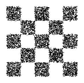
Checkerboard

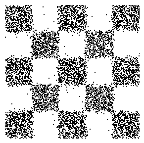
ZZP

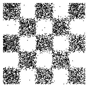
RHMC

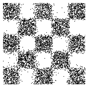
BPS

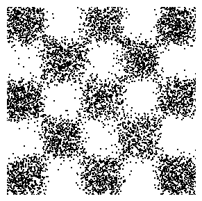
i-DDPM

Fractal tree

ZZP

RHMC

BPS

i-DDPM

Olympic rings

ZZP

RHMC

BPS

i-DDPM

Rose

ZZP

RHMC

BPS

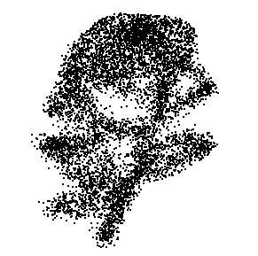
i-DDPM

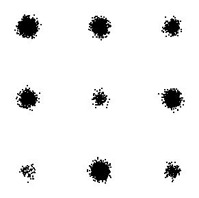
Gaussian mixture

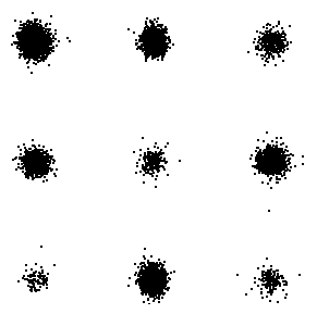
ZZP

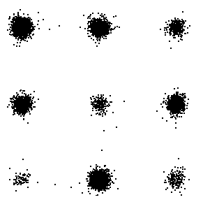
RHMC

BPS

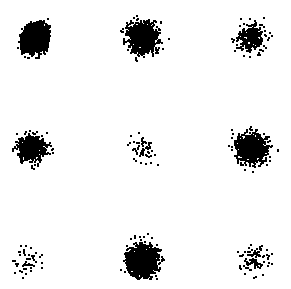
i-DDPM

Figure 3: Generation for the various datasets.

E.2 MNIST digits

Figure 4: Generation for the ZZP trained on MNIST.

Finally, we consider the task of generating handwritten digits training the ZZP on the MNIST dataset. In Figure 4 we show promising results obtained with the same design choices described in Section E.1, apart from the following differences. The optimiser is Adam [Kingma and Ba, 2015] with learning rate 2e-4. We use a U-Net following the implementation of Nichol and Dhariwal [2021], choosing the parameters of the network as follows: we set the hidden layers to $[128,256,256,256]$, fix the number of residual blocks to $2$ at each level, and add self-attention block at resolution $16\times 16$, using $4$ heads. We use an exponential moving average with a rate of $0.99$. At every layer, we use the silu activation function, while we apply the softplus to the output of the network, with $\beta=0.2$. We train the model for 40000 steps with batch size $128$.

References

- Anderson [1982] Brian D.O. Anderson. Reverse-time diffusion equation models. Stochastic Processes and their Applications, 12(3):313–326, 1982. ISSN 0304-4149. doi: https://doi.org/10.1016/0304-4149(82)90051-5.
- Berg and Brown [1972] Howard C Berg and Douglas A Brown. Chemotaxis in escherichia coli analysed by three-dimensional tracking. Nature, 239(5374):500–504, 1972.
- Bertazzi et al. [2022] Andrea Bertazzi, Joris Bierkens, and Paul Dobson. Approximations of Piecewise Deterministic Markov Processes and their convergence properties. Stochastic Processes and their Applications, 154:91–153, 2022.
- Bertazzi et al. [2023] Andrea Bertazzi, Paul Dobson, and Pierre Monmarché. Piecewise deterministic sampling with splitting schemes. arXiv.2301.02537, 2023.
- Bierkens et al. [2019a] Joris Bierkens, Paul Fearnhead, and Gareth Roberts. The zig-zag process and super-efficient sampling for bayesian analysis of big data. Annals of Statistics, 47, 2019a.
- Bierkens et al. [2019b] Joris Bierkens, Gareth O Roberts, and Pierre-André Zitt. Ergodicity of the zigzag process. The Annals of Applied Probability, 29(4):2266–2301, 2019b.
- Bou-Rabee and Sanz-Serna [2017] Nawaf Bou-Rabee and Jesús María Sanz-Serna. Randomized hamiltonian monte carlo. The Annals of Applied Probability, 27(4):2159–2194, 2017.
- Bouchard-Côté et al. [2018] Alexandre Bouchard-Côté, Sebastian J. Vollmer, and Arnaud Doucet. The Bouncy Particle Sampler: A Nonreversible Rejection-Free Markov Chain Monte Carlo Method. Journal of the American Statistical Association, 113(522):855–867, 2018.
- Chen et al. [2023] Sitan Chen, Sinho Chewi, Jerry Li, Yuanzhi Li, Adil Salim, and Anru Zhang. Sampling is as easy as learning the score: theory for diffusion models with minimal data assumptions. In The Eleventh International Conference on Learning Representations, 2023.
- Cloez, Bertrand et al. [2017] Cloez, Bertrand, Dessalles, Renaud, Genadot, Alexandre, Malrieu, Florent, Marguet, Aline, and Yvinec, Romain. Probabilistic and Piecewise Deterministic models in Biology. ESAIM: Procs, 60:225–245, 2017.
- Conforti and Léonard [2022] Giovanni Conforti and Christian Léonard. Time reversal of markov processes with jumps under a finite entropy condition. Stochastic Processes and their Applications, 144:85–124, 2022. ISSN 0304-4149. doi: https://doi.org/10.1016/j.spa.2021.10.002.
- Croitoru et al. [2023] Florinel-Alin Croitoru, Vlad Hondru, Radu Tudor Ionescu, and Mubarak Shah. Diffusion models in vision: A survey. IEEE Transactions on Pattern Analysis and Machine Intelligence, 2023.
- Davis [1984] M. H. A. Davis. Piecewise-Deterministic Markov Processes: A General Class of Non-Diffusion Stochastic Models. Journal of the Royal Statistical Society. Series B (Methodological), 46(3):353–388, 1984.
- Davis [1993] M.H.A. Davis. Markov Models & Optimization. Chapman & Hall/CRC Monographs on Statistics & Applied Probability. Taylor & Francis, 1993. ISBN 9780412314100.
- Deligiannidis et al. [2019] George Deligiannidis, Alexandre Bouchard-Côté, and Arnaud Doucet. Exponential ergodicity of the bouncy particle sampler. The Annals of Statistics, 47(3):1268–1287, 06 2019.
- Dhariwal and Nichol [2021] Prafulla Dhariwal and Alexander Quinn Nichol. Diffusion models beat GANs on image synthesis. In A. Beygelzimer, Y. Dauphin, P. Liang, and J. Wortman Vaughan, editors, Advances in Neural Information Processing Systems, 2021.
- Dockhorn et al. [2022] Tim Dockhorn, Arash Vahdat, and Karsten Kreis. Score-based generative modeling with critically-damped langevin diffusion. In International Conference on Learning Representations, 2022.
- Dumas et al. [2002] Vincent Dumas, Fabrice Guillemin, and Philippe Robert. A markovian analysis of additive-increase multiplicative-decrease algorithms. Advances in Applied Probability, 34(1):85–111, 2002. doi: 10.1239/aap/1019160951.
- Durkan et al. [2019] Conor Durkan, Artur Bekasov, Iain Murray, and George Papamakarios. Neural spline flows. In H. Wallach, H. Larochelle, A. Beygelzimer, F. d'Alché-Buc, E. Fox, and R. Garnett, editors, Advances in Neural Information Processing Systems, volume 32. Curran Associates, Inc., 2019.
- Durmus et al. [2020] Alain Durmus, Arnaud Guillin, and Pierre Monmarché. Geometric ergodicity of the Bouncy Particle Sampler. The Annals of Applied Probability, 30(5):2069–2098, 10 2020.
- Durmus et al. [2021] Alain Durmus, Arnaud Guillin, and Pierre Monmarché. Piecewise deterministic Markov processes and their invariant measures. Annales de l’Institut Henri Poincaré, Probabilités et Statistiques, 57(3):1442 – 1475, 2021.
- Embrechts and Schmidli [1994] Paul Embrechts and Hanspeter Schmidli. Ruin estimation for a general insurance risk model. Advances in Applied Probability, 26(2):404–422, 1994.
- Fearnhead et al. [2018] Paul Fearnhead, Joris Bierkens, Murray Pollock, and Gareth O. Roberts. Piecewise deterministic markov processes for continuous-time monte carlo. Statistical Science, 33(3):386–412, 08 2018.
- Ho et al. [2020] Jonathan Ho, Ajay Jain, and Pieter Abbeel. Denoising diffusion probabilistic models, 2020.
- Hyvärinen [2005] Aapo Hyvärinen. Estimation of non-normalized statistical models by score matching. Journal of Machine Learning Research, 6(24):695–709, 2005.
- Hyvärinen [2007] Aapo Hyvärinen. Some extensions of score matching. Comput. Stat. Data Anal., 51:2499–2512, 2007.
- Jacobsen [2005] M. Jacobsen. Point Process Theory and Applications: Marked Point and Piecewise Deterministic Processes. Probability and Its Applications. Birkhäuser Boston, 2005. ISBN 9780817642150.
- Jeong et al. [2021] Myeonghun Jeong, Hyeongju Kim, Sung Jun Cheon, Byoung Jin Choi, and Nam Soo Kim. Diff-TTS: A Denoising Diffusion Model for Text-to-Speech. In Proc. Interspeech 2021, pages 3605–3609, 2021. doi: 10.21437/Interspeech.2021-469.
- Kingma and Ba [2015] Diederik Kingma and Jimmy Ba. Adam: A method for stochastic optimization. In International Conference on Learning Representations (ICLR), San Diega, CA, USA, 2015.
- Kong et al. [2021] Zhifeng Kong, Wei Ping, Jiaji Huang, Kexin Zhao, and Bryan Catanzaro. Diffwave: A versatile diffusion model for audio synthesis. In International Conference on Learning Representations, 2021.
- Lou et al. [2024] Aaron Lou, Chenlin Meng, and Stefano Ermon. Discrete diffusion modeling by estimating the ratios of the data distribution. arXiv:2310.16834, 2024.
- Neal [2010] Radford M. Neal. MCMC using Hamiltonian dynamics. Handbook of Markov Chain Monte Carlo, 54:113–162, 2010.
- Nichol and Dhariwal [2021] Alexander Quinn Nichol and Prafulla Dhariwal. Improved denoising diffusion probabilistic models. In Marina Meila and Tong Zhang, editors, Proceedings of the 38th International Conference on Machine Learning, volume 139 of Proceedings of Machine Learning Research, pages 8162–8171. PMLR, 18–24 Jul 2021.
- Papamakarios et al. [2021] George Papamakarios, Eric Nalisnick, Danilo Jimenez Rezende, Shakir Mohamed, and Balaji Lakshminarayanan. Normalizing flows for probabilistic modeling and inference. Journal of Machine Learning Research, 22(57):1–64, 2021.
- Paszke et al. [2019] Adam Paszke, Sam Gross, Francisco Massa, Adam Lerer, James Bradbury, Gregory Chanan, Trevor Killeen, Zeming Lin, Natalia Gimelshein, Luca Antiga, Alban Desmaison, Andreas Köpf, Edward Yang, Zach DeVito, Martin Raison, Alykhan Tejani, Sasank Chilamkurthy, Benoit Steiner, Lu Fang, Junjie Bai, and Soumith Chintala. Pytorch: An imperative style, high-performance deep learning library, 2019.
- Rozet et al. [2022] François Rozet et al. Zuko: Normalizing flows in pytorch, 2022.
- Song et al. [2021] Yang Song, Jascha Sohl-Dickstein, Diederik P Kingma, Abhishek Kumar, Stefano Ermon, and Ben Poole. Score-based generative modeling through stochastic differential equations. In International Conference on Learning Representations, 2021.
- Sugiyama et al. [2011] Masashi Sugiyama, Taiji Suzuki, and Takafumi Kanamori. Density ratio matching under the bregman divergence: A unified framework of density ratio estimation. Annals of the Institute of Statistical Mathematics, 64, 10 2011. doi: 10.1007/s10463-011-0343-8.
- Sun et al. [2023] Haoran Sun, Lijun Yu, Bo Dai, Dale Schuurmans, and Hanjun Dai. Score-based continuous-time discrete diffusion models. In The Eleventh International Conference on Learning Representations, 2023.
- Vincent [2011] Pascal Vincent. A connection between score matching and denoising autoencoders. Neural computation, 23(7):1661–1674, 2011.
- Zhang et al. [2008] Huilong Zhang, François Dufour, Y. Dutuit, and Karine Gonzalez. Piecewise deterministic markov processes and dynamic reliability. Proceedings of the Institution of Mechanical Engineers, Part O: Journal of Risk and Reliability, 222:545–551, 12 2008. doi: 10.1243/1748006XJRR181.