Three-dimensional solitons supported by the spin-orbit coupling and Rydberg-Rydberg interactions in $\mathcal{PT}$-symmetric potentials

Abstract

Excited states (ESs) of two- and three-dimensional (2D and 3D) solitons of the semivortex (SV) and mixed-mode (MM) types, supported by the interplay of the spin-orbit coupling (SOC) and local nonlinearity in binary Bose-Einstein condensates, are unstable, on the contrary to the stability of the SV and MM solitons in their fundamental states. We propose a stabilization strategy for these states in 3D, combining SOC and long-range Rydberg-Rydberg interactions (RRI), in the presence of a spatially-periodic potential, that may include a parity-time ($\mathcal{PT}$)-symmetric component. ESs of the SV solitons, which carry integer vorticities $S$ and $S+1$ in their two components, exhibit robustness up to $S=4$. ESs of MM solitons feature an interwoven necklace-like structure, with the components carrying opposite fractional values of the orbital angular momentum. Regions of the effective stability of the 3D solitons of the SV and MM types (both fundamental ones and ESs), are identified as functions of the imaginary component of the $\mathcal{PT}$-symmetric potential and strengths of the SOC and RRI terms.

1 Introduction

The formation of multidimensional solitons holds fundamental significance across various domains of physics, including nonlinear optics [1, 2, 3, 4, 5], Bose-Einstein condensates (BECs) [6, 7, 8, 9], superconductors [10], semiconductors [11], ferromagnetic media [12], and general field theory [13, 14]. Unlike one-dimensional (1D) solitons, which emerge, normally, as stable modes, looking for stable 2D and, especially, 3D solitons is a challenging problem [15]. Indeed, the prerequisite for the formation of solitons is the presence of an attractive (or self-focusing) nonlinearity. However, the ubiquitous cubic self-attraction gives rise to the destabilizing critical and supercritical wave collapse in the 2D and 3D geometry, respectively [16, 17]. Solitons with embedded vorticity are subject to a still stronger splitting azimuthal modulational instability [18].

Various stabilization scenarios for fundamental and vortex multidimensional solitons have been elaborated [15]. These include the use of saturable or competing nonlinearities [19, 20], nonlocal nonlinearity [21, 22], and special nonlinear interactions [23, 24]. Additionally, the stabilization of multidimensional solitons may occur in optical tandem systems [25], waveguide arrays and optical lattices embedded in various materials [26, 27, 28, 29, 30], and long-range interactions between Rydberg atoms [21, 31]. More recently, stable 2D and 3D solitons were predicted, respectively, as ground [32, 33, 34] or metastable [35] states in binary Bose-Einstein condensates (BECs) carrying spin-orbit coupling (SOC).

SOC BECs, experimentally realized in Ref. [36], have attracted much interest due to their potential for realizing phenomena induced by the artificial gauge potential [37]. These settings give rise to various matter-wave modes, such as vortices [38, 39], monopoles [40], multi-domain patterns [41], quantum droplets [42, 43, 44, 45, 46], and solitons [47]-[52]. Further, Ref. [49] has predicted various self-trapped vortex-soliton complexes in the 2D binary-BEC model with the Rashba-type SOC and attractive intrinsic nonlinearity. Refs. [50] and [51] have used systems with spatially confined SOC in BEC as localized gauge potentials, examining properties of the respective soliton complexes and spinor dynamics. As demonstrated in Ref. [35], a self-attractive binary SOC condensate can sustain metastable 3D solitons in the free space, in spite of the absence of a ground state, which does not exist in the system admitting the supercritical collapse. The study indicates that the SOC-induced change of the 3D condensate’s dispersion may balance the attractive nonlinearity, resulting in the formation of the solitons which are stable against small perturbations.

A generic approach relies on the use of spatially periodic potentials, which secure the stabilization of multidimensional solitons [53, 54]. Furthermore, in the case of the local self-repulsive nonlinearity, stable gap solitons exist in spectral bandgaps created by such periodic potentials [9, 55, 56]. The stabilization of solitons can be enhanced by fine-tuning the nonlinearities and magnitude of the external potentials. Notably, the incorporation of parity-time ($\mathcal{PT}$) symmetry into periodic potentials has been demonstrated as an effective technique for generating a variety of optical solitons. This is achieved by adding an imaginary spatially-odd component to the spatially-even real periodic potential [57, 58, 59, 60, 61]. Recently, Ref. [62] addressed 3D solitons in complex $\mathcal{PT}$-symmetric periodic lattices combined with the focusing Kerr nonlinearity. It was found that such lattices are capable to stabilize both fundamental and vortex soliton states.

Cold Rydberg atoms offer a powerful platform for the generation of stable multidimensional solitons, both fundamental and vortical ones [38, 39]. The long-range Rydberg-Rydberg interaction (RRI) gives rise to a nonlocal optical nonlinearity via the effect of the electromagnetically induced transparency, producing a significant impact even at the single-photon level [58]. This line of the studies has led to the prediction of numerous optical phenomena, including stable storage and retrieval of light bullets [31], their two-component counterparts [63], controllable bound states of the bullets [64], transient optical responses [65], and effective photon interactions [66]. The extended lifetimes of Rydberg atomic states, on the order of tens of microseconds, secure the coherence of the resultant optical nonlinearities. These characteristics position Rydberg systems as nearly ideal candidates for the development of advanced photonic devices, such as single-photon switches and transistors [67, 68], quantum memory units, and phase gates [69, 70].

Despite recent advancements, 3D vortex solitons in binary condensates, which are supported by the interplay of SOC and RRI in the presence of the spatially potentials, real or $\mathcal{PT}$-symmetric ones, are not yet fully understood. The objective of the present work is to systematically construct 3D stable solitons in the binary SOC BEC, in conjunction with mean-field interactions and $\mathcal{PT}$-symmetric potentials, through a comprehensive numerical analysis. We demonstrate the existence of 3D stable solitons of the semivortex (SV) and mixed-mode (MM) types. In particular, for the 3D SV solitons with integer vorticities $\left(S,S+1\right)$ in their two components, such results are reported for $S\leq 4$, i.e., essentially, for higher-order solitons (alias excited states (ESs) of the fundamental solitons, which correspond solely to $S=-1$ and $S=0$). Our findings reveal that the imaginary component of the $\mathcal{PT}$ symmetry potential, along with the SOC and RRI strengths significantly affect the structure and stability domains of the two types (SV and MM) of the higher-order solitons.

2 The spin-orbit-coupled condensate of Rydberg atoms

In this work, we aim to predict robust SV and MM solitons in the 3D SOC BEC system, under the action of a $\mathcal{PT}$-symmetric potential. To this end, we consider matter waves in Rydberg atomic gases, where the interplay between the $\mathcal{PT}$ symmetry and RRI may give rise to novel soliton phenomenology. With the help of a systematic numerical analysis, we explore the shape and stability of the solitons.

The mean-field dynamics of the two-component wave function of the binary BEC is governed by the spinor Gross-Pitaevskii equation (GPE),

$$i\hbar\frac{\partial\psi_{+}}{\partial t}=\left[-\frac{\hbar^{2}}{2M}\nabla^{2}+\left(g_{11}\left|\psi_{+}\right|^{2}+g_{12}\left|\psi_{-}\right|^{2}\right)+V_{\mathrm{SO}}+V_{\mathcal{PT}}({\mathbf{r}})\right.$$

$$\left.+\int{\mathrm{d}^{3}{\mathbf{r}}^{\prime}\left(U_{11}\left|\psi_{+}\right|^{2}+U_{12}\left|\psi_{-}\right|^{2}\right)}\right]\psi_{+},$$

$$i\hbar\frac{\partial\psi_{-}}{\partial t}=\left[-\frac{\hbar}{2M}\nabla^{2}+\left(g_{21}\left|\psi_{-}\right|^{2}+g_{22}\left|\psi_{+}\right|^{2}\right)-V_{\mathrm{SO}}+V_{\mathcal{PT}}({\mathbf{r}})\right.$$

$$\left.+\int{\mathrm{d}^{3}{\mathbf{r}}^{\prime}\left(U_{21}\left|\psi_{-}\right|^{2}+U_{22}\left|\psi_{+}\right|^{2}\right)}\right]\psi_{-},$$ (1)

where $\psi=(\psi_{+},\psi_{-})$ are two components of the spinor wave functions, ${\mathbf{r}}=(x,y,z)$, $\nabla^{2}={\partial^{2}}/{\partial x^{2}}+{\partial^{2}}/{\partial y^{2}}+{\partial^{2}}/{\partial z^{2}}$, $M$ is the atomic mass, and $g_{ij}(i,j=1,2)$ are strengths of local intra- and inter-component contact interactions. In this work, we consider local interactions which are symmetric with respect to the components, with $g_{11}=g_{22}=g_{12}=g_{21}=4\pi\hbar^{2}a_{s}/M$, where $a_{s}$ is $s$-wave scattering strength. The Rashba-type SOC operator with strength $\lambda$ is represented by $V_{\mathrm{SO}}\psi_{+}=i\lambda\left(\partial\psi_{-}/\partial x-i\partial\psi_{-}/\partial y+\partial\psi_{+}/\partial z\right)$ and $V_{\mathrm{SO}}\psi_{-}=i\lambda\left(\partial\psi_{+}/\partial x+i\partial\psi_{+}/\partial y-\partial\psi_{-}/\partial z\right)$. The $\mathcal{PT}$-symmetric potential is taken as

$$V_{\mathcal{PT}}({\mathbf{r}})=p_{r}\left[\cos^{2}(\omega x)+\cos^{2}(\omega y)+\cos^{2}(\omega z)\right]+ip_{i}\left[\sin(\omega x)+\sin(\omega y)+\sin(\omega z)\right],$$ (2)

where $p_{r}$ and $p_{i}$ are strengths of its real and imaginary parts, which are even and odd functions of the coordinates, respectively. As shown below, the presence of the real part of the potential is necessary for the effective stability (robustness) of the 3D solitons, while the imaginary part actually produces a destabilizing effect.

The nonlocal RRI potential in the last term of Eq. (1) is written as $U_{jk}(\mathbf{r}^{\prime}-\mathbf{r})=C_{6}^{(jk)}\left/\left(R_{b}^{6}+\left|\mathbf{r}^{\prime}-\mathbf{r}\right|^{6}\right)\right.$, with $U_{12}=U_{21}$, where $C_{6}^{(jk)}$ are effective coefficients of the van der Waals interaction, $R_{b}$ being the Rydberg-blockade radius. Further, we adopt dimensionless units by means of scaling variables with respect to the relevant length and time units, $R_{b}$ and $\tau_{b}=R_{b}^{2}M/\hbar$. Then Eq. (1) is replaced by the normalized GPE,

$$i\frac{\partial\psi_{+}}{\partial t}=\left[-\frac{1}{2}\nabla^{2}+\gamma\left(\left|\psi_{+}\right|^{2}+\left|\psi_{-}\right|^{2}\right)+V_{\mathrm{SO}}+V_{\mathcal{PT}}({\mathbf{r}})\right.$$

$$\left.+\int{\mathrm{d}^{3}{\mathbf{r}}^{\prime}\tilde{U}({\mathbf{r}}-{\mathbf{r}}^{\prime})\left(\alpha_{11}\left|\psi_{+}\right|^{2}+\alpha_{12}\left|\psi_{-}\right|^{2}\right)}\psi_{+}\right],$$

$$i\frac{\partial\psi_{-}}{\partial t}=\left[-\frac{1}{2}\nabla^{2}+\gamma\left(\left|\psi_{-}\right|^{2}+\left|\psi_{+}\right|^{2}\right)-V_{\mathrm{SO}}+V_{\mathcal{PT}}({\mathbf{r}})\right.$$

$$\left.+\int{\mathrm{d}^{3}{\mathbf{r}}^{\prime}\tilde{U}({\mathbf{r}}-{\mathbf{r}}^{\prime})\left(\alpha_{21}\left|\psi_{-}\right|^{2}+\alpha_{22}\left|\psi_{+}\right|^{2}\right)}\right]\psi_{-}.$$ (3)

Here $\tilde{U}({\mathbf{r}}-{\mathbf{r}}^{\prime})=1/\left[1+({\mathbf{r}}-{\mathbf{r}}^{\prime})^{6})\right]$ is the RRI kernel, dimensionless RRI coefficients are

$$\alpha_{jk}=-MNC_{6}^{(jk)}/(\hbar^{2}R_{b}^{4}),$$ (4)

the contact-interaction strength is set as $\gamma=1$ by scaling, along with $M=\hbar=1$, and $N$ is the number of atoms in this system, defined as $N=N_{+}+N_{-}$, where $N_{+}=\int{\left|\psi_{+}({\mathbf{r}})\right|^{2}\mathrm{d}^{3}{\mathbf{r}}}$ and $N_{-}=\int{\left|\psi_{-}({\mathbf{r}})\right|^{2}\mathrm{d}^{3}{\mathbf{r}}}$ are norms of the two components of wave function.

The system’s energy, which corresponds to Eq. (3), is

$$\begin{split}E_{\mathrm{tot}}&=\int{\ \left(\varepsilon_{k}+\varepsilon_{\mathrm{SOC}}+\varepsilon_{\mathrm{local}}+\varepsilon_{\mathrm{SC}}+\varepsilon_{\mathrm{ext}}\right)\mathrm{d}^{3}{\mathbf{r,}}}\\ \varepsilon_{k}&=\frac{1}{2}\left(\left|\nabla\psi_{+}\right|^{2}+\left|\nabla\psi_{-}\right|^{2}\right),\\ \varepsilon_{\mathrm{SOC}}&=\lambda\left[\psi_{+}^{\ast}\left({\frac{{\partial\psi_{-}}}{{\partial x}}}-i{\frac{{\partial\psi_{-}}}{{\partial y}}}+{\frac{{\partial\psi_{+}}}{{\partial z}}}\right)-\psi_{-}^{\ast}\left({\frac{{\partial\psi_{+}}}{{\partial x}}}+i{\frac{{\partial\psi_{+}}}{{\partial y}}}-{\frac{{\partial\psi_{-}}}{{\partial z}}}\right)\right],\\ \varepsilon_{\mathrm{local}}&=\frac{1}{2}\gamma\left(|\psi_{+}|^{4}+|\psi_{-}|^{4}+2|\psi_{+}|^{2}|\psi_{-}|^{2}\right),\\ \varepsilon_{\mathrm{RRI}}&=\frac{1}{2}|\psi_{+}|^{2}\int{\mathrm{d}^{3}{\mathbf{r}}^{\prime}\left(\alpha_{11}\tilde{U}_{11}\left|\psi_{+}\right|^{2}+\alpha_{12}\tilde{U}_{12}\left|\psi_{-}\right|^{2}\right)}\\ &+\frac{1}{2}|\psi_{-}|^{2}\int{\mathrm{d}^{3}{\mathbf{r}}^{\prime}\left(\alpha_{21}\tilde{U}_{21}\left|\psi_{-}\right|^{2}+\alpha_{22}\tilde{U}_{22}\left|\psi_{+}\right|^{2}\right),}\\ \varepsilon_{\mathrm{ext}}&=\frac{1}{2}V_{\mathcal{PT}}({\mathbf{r}})\left(|\psi_{+}|^{2}+|\psi_{-}|^{2}\right),\end{split}$$ (5)

where $\varepsilon_{k}$, $\varepsilon_{\mathrm{SOC}}$, $\varepsilon_{\mathrm{local}}$, $\varepsilon_{\mathrm{RRI}}$, and $\varepsilon_{\mathrm{ext}}$ represent the kinetic, SOC, local (contact), nonlocal (RRI), and external potential energies, respectively. The above condition $\gamma=1$ and Eq. (4) imply that we consider the system with local repulsion, while the long-range RRI may be both attractive and repulsive. In the case when all nonlinear interactions are repulsive and the periodic potential is present, multidimensional self-trapped states may exist as gap solitons [15].

For experimental consideration, this model can be realized, in particular, in an ultracold gas of ${}^{88}\mathrm{Sr}$ atoms [31]. In that case, relevant values of the physical parameters are $C_{6}=2\pi\times 81.6~{}\mathrm{GHz}\cdot\mathrm{\mu m}^{6}$, $R_{b}=10~{}\mathrm{\mu m}$, and $\tau=0.18~{}\mathrm{s}$.

3 The results and discussions

Stationary solution of Eq. (3) are looked for in the usual form, $\psi_{\pm}=\phi_{\pm}e^{-i\mu t}$, where $\mu$ is the chemical potential, and $\phi_{\pm}$ are components of the stationary wave function. In the polar coordinates ($r,\theta$), the initial ansatz [35, 71] for the 3D SV mode is

$$\phi_{\pm}=A_{\pm}r^{S_{\pm}}\exp(-a_{\pm}r^{2}+iS_{\pm}\theta),$$ (6)

and for the MM one it is

$$\phi_{\pm}=A_{1}r^{\left|S_{1}\right|}\exp(-a_{1}r^{2}\pm iS_{1}\theta)\mp A_{2}r^{\left|S_{2}\right|}\exp(-a_{2}r^{2}\mp iS_{2}\theta).$$ (7)

Here $S_{-}=S_{+}+1$ and $S_{2}=S_{1}+1$ are the corresponding vorticities, $A_{\pm}$, $A_{1}$ and $A_{2}$ are amplitudes of the components, and $a_{\pm}$, $a_{1}$, and $a_{2}$ are positive parameters. Below, the components corresponding to signs $+$ and $-$ in Eqs. (6) and (7) are referred to as SV+, SV- and MM+, MM-, respectively.

As mentioned above, the fundamental SV states are produced by $(S_{+},S_{-})=(-1,0)$ and $(S_{+},S_{-})=(0,1)$, while the ESs correspond to the other integer values of $S_{+}$ and $S_{-}$. Similarly, for the MM-type ansatz, the fundamental states correspond to $(S_{1},S_{2})=(-1,0)$ and $(S_{1},S_{2})=(0,1)$. One component with topological charge equal to $0$ represents the fundamental solitons, and the other component represents the excited state. Thus, the whole state is called fundamental state. For the other cases, none of the component possess zero topological charge, the two components are both excited states, and the whole state is called excited states. The differences between the fundamental and excited states lie in the norm. Generally, the solitons with fundamental state has lower norm.

In the 3D SOC system, stable 3D solitons are hard to generate. Nevertheless, 3D robust (quasi-stable) solitons can be obtained in the system including RRI and the $\mathcal{PT}$-symmetric potential. The 3D SV and MM solitons can be generated and exist for a finite time, but they undergo nonvanishing evolution and eventually collapse at large times. The robustness of these solitons can be quantified by changes of their norm and shape during the evolution. Robust 3D solitons of the SV and MM types, both fundamental (with $S_{+,1}=0$) and ES ones (with $S_{+,1}\geq 1$), are found by means of the imaginary-time integration method [72, 73]. Typical examples of the 3D robust solitons of these types are shown in Figs. 1 and 2, where the soliton profiles are obtained from the analytical ansätze (6) and (7).

3.1 The robustness and evolution of the 3D SV and MM solitons

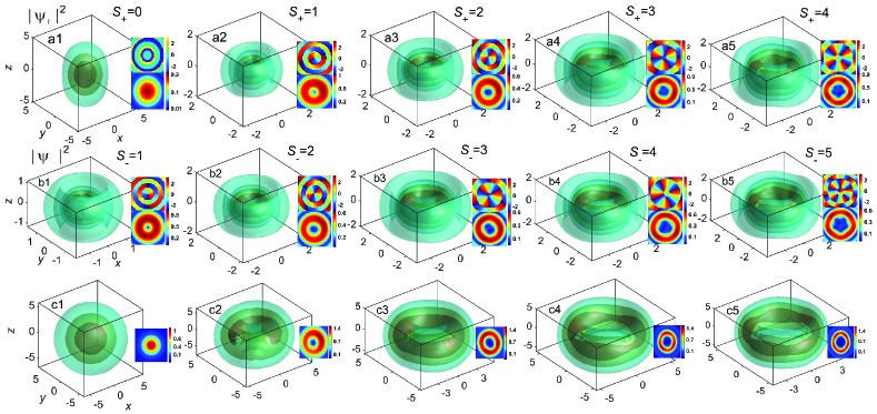
Figure 1: The density distribution in the SV type solitons. The intensities of three isosurface layers correspond to $85\%$, $50\%$, and $5\%$ of the maximum value (in other figures density isosurfaces are plotted according to the same definition). The first to third lines display, respectively, the SV+ sand SV- components, and the total density of both components. The vorticity $S_{+}$ from the first to fifth columns are 0$\sim$4, and $S_{-}=S_{+}+1$. The insets are the corresponding phase and density distributions in the ($x,y$) plane. The parameters for the SVs are given in Tab. 1.

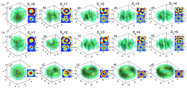
Figure 2: MM solitons with MM+ and MM-types. The topological charges from the first to the fourth column are $S_{1}=0,1,2,3,4$ and $S_{2}=S_{1}+1$. The first to the fifth rows are MM+, MM- components, and total modes, respectively. The parameters for MMs are given in Tab. 1.

For $(S_{+},S_{-})=(0,1)$, the SV+ and SV- components are the fundamental and vortical ones, as shown in panels (a1) and (b1) of the first column of Fig. 1. Vorticities $(S_{+},S_{-})$ of the ESs are $(1,2)$, $(2,3)$, $(3,4)$, and $(4,5)$ in the second to fifth columns in Fig. 1. For ESs, both components of SVs are vortical ones. The simulations have demonstrated that SOC BEC system can support robust 3D SV solitons with vorticities $S_{+}\leq 4$. A typical example of the soliton evolution for $S_{+}=2$, performed by means of the split-step Fourier method up to $t=500$, is presented in Fig. 3. In the course of this simulation, the total norm of the SV soliton is strictly conserved. The consideration of Fig. 3 demonstrates that the SV soliton stays fully robust up $t=300$. In physical units, this time is $\simeq 40$ s, which is definitely sufficient for the experimental observation. The parameters for robust SVs in Fig. 1 are presented in Tab. 1, where the control parameters are SOC strength $\lambda$, amplitudes of the real and imaginary parts of the $\mathcal{PT}$-symmetric potential (2), $p_{r}$ and $p_{i}$, and RRI strengths $\alpha_{jk}$.

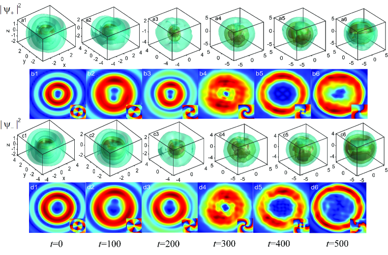
Figure 3: The evolution of the density and phase distributions in two components of a typical 3D SV soliton with $S_{+}=2$. The snapshots are displayed at times $t=0,100,200,300,400,500$. The other parameters are: $\lambda=3$, $p_{r}=-0.1$, $p_{i}=0.02$, and $\alpha_{11}=\alpha_{12}=\alpha_{21}=\alpha_{22}=0.1$.

At $S_{+}>4$, the SVs are not robust anymore. A typical example of the evolution of an unstable SV, with vorticities $(S_{+},S_{-})=(5,6)$, is shown in Fig. 4. In this case, the SV lasts until $z=50$ ($\simeq 9$ s, in physical units), which is significantly shorter than in the case of the robust SV solitons with $S_{+}\leq 4$.

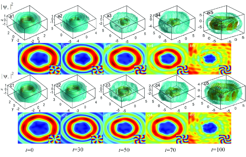
Figure 4: The evolution of typical example of unrobust 3D SV solitons with $(S_{+},S_{-})=(5,6)$. The snapshots are displayed at times $t=0,10,50,70,100$. The other parameters are the same as Fig. 3.

For the MM ansatz, the system is also capable of supporting both fundamental and ES solitons in 3D. The respective density distributions are plotted in Fig. 2. The fundamental state is presented in the first column, corresponding to vorticities $(S_{1},S_{2})=(0,1)$. The subsequent columns, ranging from the second to the fifth one, show ESs with $(S_{1},S_{2})=(1,2),(2,3),(3,4),(4,5)$.

In contrast to SVs, MMs exhibit quasi-discrete necklace-shaped distributions around a central ring. The number of the discrete cores is given by $N_{c}=2S_{1}+1$, with $S_{1}$ denoting the vorticity of the MM+ component. Note that the densities of the MM+ and MM- components are shaped in alternating patterns along the ring, hence the total density distribution of the MM solitons features a smooth ring-like configuration.

A typical example of the robust evolution of a 3D MM soliton with vorticity $S_{1}=2$ is displayed in Fig. 5. As well as in the case of the SV soliton shown in Fig. 3, the evolution is shown up to $t=500$, and it can be concluded that the it stays fully robust up to $t=300$, i.e., time $\simeq 40$ s in physical units, Also similar to the result for the SV soliton, the norm of the MM one is strictly conserved in the course of the evolution.

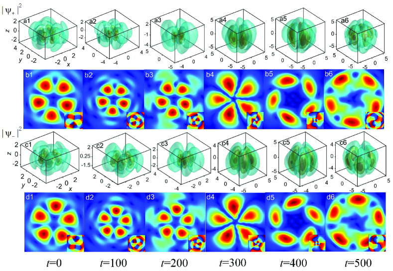
Figure 5: The same as in Fig. 3, but for a typical 3D soliton of the MM type with vorticity $S_{1}=2$. The parameters are the same as in Fig. 3.

Table 1: Parameters for robust SVs and MMs of the fundamental and ES types.

Topological charge	$\lambda$	$p_{r}$	$p_{i}$	$\alpha_{jk}$
SVs ($S_{+}$, $S_{-}$)
(0, 1)	3.8	-0.1	0.01	1
(1, 2)	4	-0.1	0.02	1
(2, 3)	3	-0.1	0.02	1
(3, 4)	3	-0.1	0.01	1
(4, 5)	3.5	-0.1	0.01	1
MMs ($S_{1}$, $S_{2}$)
(0, 1)	2.8	-0.1	0.01	1
(1, 2)	3.2	-0.1	0.01	1
(2, 3)	2.3	-0.1	0.02	1
(3, 4)	2.7	-0.1	0.02	1
(4, 5)	3.3	-0.1	0.01	1

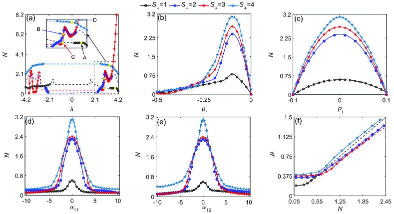
Figure 6: The norm of the SV-type solitons as a function of (a) SOC strength $\lambda$, amplitudes pf real (b) and imaginary (c) parts of the $\mathcal{PT}$-symmetric potential (2), (d) intra- and (e) inter-component RRI strength, (f) chemical potential $\mu$. The inset in (a) is the zoom of region $\lambda\in(2.0~{}4.2)$, where points A, B, C and D designate states correspond to the SVs with vorticities $S_{+}=1,2,3,4$ in Fig.  1. Solid and dashed lines represent robust and strongly unstable SVs, respectively. The fixed parameters for each panel are presented in Tab. 1.

The modulation of SVs following the variation of the system’s parameters, such as the SOC constant $\lambda$, amplitudes of the real and imaginary parts of the potential, intra- and inter-component of RRI strengths, as well as the dependence between the chemical potential $\mu$ and total norm, are shown in Fig. 6. The $N(\lambda)$ relations displayed in Fig. 6(a) delineate robustness domains for the SV solitons for different vorticities. It is seen that the domains are divided in two distinct regions, situated, respectively, at $\lambda<0$ and $\lambda>0$, indicating this system cannot support robust SVs unless the SOC strength $|\lambda|$ exceeds a certain threshold value. Details of the robustness domains are summarized in Tab. 2. SVs do not remain either if the SOC strength is too large, viz., at $\left|\lambda\right|>4.2$.

For different vorticities, the SV norms exhibit different behavior for the variation of $\lambda$. For $S_{+}=1$ and $4$, the norm changes smoothly with $\lambda$, while it strongly fluctuates for $S_{+}=2$ and $3$. For example, $N$ changes by $\simeq 10$ times when $\lambda$ varies from $3.2$ to $4.2$ for $S_{+}=3$. The increase of the vorticity enhances the fluctuations of the norm, eventually leading to full instability of SVs at $S_{+}\geq 5$ (as mentioned above). The parameter dependence for the 3D MM solitons is similar to that for SVs (not shown here in detail).

The dependence of the gap of values of the SOC constant$\ \lambda$, which divides the robustness domain at $\lambda<0$ and $\lambda>0$, on parameters $p_{i}$ and $\alpha_{12}$ is shown in Fig. 7. Here $S_{+}=3$ for SVs and $S_{1}=3$ for MMs, the other parameters being $p_{r}=-0.1$, $\alpha_{11}=\alpha_{22}=1$.

Amplitudes of the real and imaginary parts of the $\mathcal{PT}$-symmetric potential are essential parameters which control the robust SV solitons. Figures 6(b) and (c) display the soliton’s norm vs. $p_{r}$ and $p_{i}$. It is seen that only $p_{r}<0$ can support robust SVs, as in the opposite case the soliton is placed at a local potential maximum, instead of the minimum (see Eq. (2)). On the other hand, there is natural symmetry between positive and negative values of $p_{i}$. Taking Fig. 1 and Tab. 2 for example, with fixed parameters $(S_{+},\lambda,\alpha_{ij},p_{r})=(2,3,1,-0.1)$, one obtains the SV soliton solutions with real chemical potential $\mu$ in the interval of $-0.1<p_{i}<+0.1$. In this case, $p_{i}=\pm 0.1$ are $\mathcal{PT}$-symmetry-breaking points [60, 61] beyond which the stationary solutions are unphysical, featuring formally complex values of $\mu$. The norm attains its maximum for the real potential, with $p_{i}=0$, and decreases with the increase of $\left|p_{i}\right|$. Actually, $\mathcal{PT}$ symmetry remains unbroken at $\left|p_{i}/p_{r}\right|<1$.

Table 2: Robustness domains for the 3D SV solitons

$(S_{+},S_{-})$	$\lambda$	$p_{r}$	$p_{i}$	$\alpha_{jk}$
(1, 2)	-4.2$\sim$ -2, 3.5$\sim$4.2	-0.5$\sim$0	-0.1 $\sim$ 0.1	-10 $\sim$ 10
(2, 3)	-2.4$\sim$ -2.2, 2.3$\sim$3.6	-0.5$\sim$0	-0.1 $\sim$ 0.1	-10 $\sim$ 10
(3, 4)	-3.9$\sim$ -3, 2.7$\sim$4.2	-0.5$\sim$0	-0.1 $\sim$ 0.1	-10 $\sim$ 10
(4, 5)	-4.2$\sim$ -2.6, 2.6$\sim$4.2	-0.5$\sim$0	-0.1 $\sim$ 0.1	-10 $\sim$ 10

The norm of the SV solitons are shown, as a functions of the intra- and inter-component RRI strengths, $\alpha_{11}$ and $\alpha_{12}$, in Figs. 6(d) and (e), respectively. It is seen that the attractive ($\alpha_{jk}<0$) and repulsive ($\alpha_{jk}>0$) interactions have approximately the same effect on the modulation of the SV solitons. Furthermore, the effect is nearly the same for the intra- and inter-component RRI strength, $\alpha_{11}$ and $\alpha_{12}$. Note that, quite naturally, the norm of the SV solitons nearly vanishes for very strong RRI, $\left|\alpha_{ij}\right|>10$.

The $\mu(N)$ curves which are displayed, for different values of $S_{+}$, in Fig. 6(f), satisfy the anti-Vakhitov-Kolokolov criterion, i.e., $\mathrm{d}\mu/\mathrm{d}N>0$, which is a known necessary condition for the stability of bright solitons supported by self-repulsive nonlinearities [74] (the Vakhitov-Kolokolov criterion proper, $\mathrm{d}\mu/\mathrm{d}N<0$ [75, 16, 17], is necessary for stability of solitons in the case of the attractive nonlinearity).

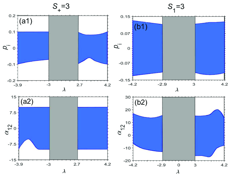
Figure 7: Blue areas: the robustness domains in paraneter planes($\lambda,p_{i}$) and ($\lambda,\alpha_{12}$). The first column is for the 3D SV solitons with $S_{+}=3$, and the second column is for the MMs with $S_{1}=3$. Gray areas represent gaps which separate the robustness domains and $\lambda<0$ and $\lambda>0$.

3.2 The energy and orbital angular momentum of SVs and MMs

The families of the 3D solitons of the SV and MM types with different vorticities can be naturally characterized by dependences of the total energy (5) on the total norm $N$, which are plotted in Figs. 8(a) and (d), respectively. It is seen that the energy increases as a function of $N$ and vorticity. Another characteristic of the spinor solitons is the orbital angular momentum (OAM) ,

$$\begin{split}\left\langle L_{\pm}\right\rangle&=\int{\mathrm{d}^{3}{\mathbf{r}}\frac{\psi_{\pm}^{\ast}{\hat{L}}\psi_{\pm}}{N_{\pm}}}\\ \left\langle L\right\rangle&=\frac{N_{+}\left\langle L_{+}\right\rangle+N_{-}\left\langle L_{-}\right\rangle}{N}\end{split}$$ (8)

where components $L_{\pm}$ should be calculated with the OAM operator ${\hat{L}}=-i(x\partial/\partial y-y\partial/\partial x)$ [33]. Figure 8(b) displays the $\left\langle L_{+}\right\rangle(N)$ relations for SVs. The orbital angular moment of atoms is proportional to the vorticity (topological charge). Due to its definition (8), $\left\langle L_{+}\right\rangle$ takes the integer value which is equal to the vorticity, $\left\langle L_{+}\right\rangle=S_{+}$, and it does not depend on the norm. Similarly, one obtains $\left\langle L_{-}\right\rangle=S_{-}$ for the second SV component, as shown in Fig. 8(c). According to Eq. 8, the total OAM is $\left\langle L\right\rangle=\left\langle L_{+}\right\rangle+0.5$. Here, the energies and OAM are calculated from ansätze (6) and (7).

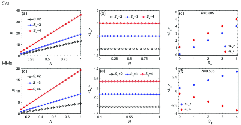
Figure 8: The energy (a,d) and OAM (b,e) as functions of the total norm for the 3D solitons of the SV and MM types. (c,f) Values of OAM for different forticities with a fixed norm. The black, blue and red lines in panels (a,b,d,e) correspond to vorticities $S_{+}=S_{1}=2,3,4$, respectively. The parameters are given in Tab. 1.

For MMs, the energy increases as a function of the norm and vorticity, as shown in Fig. 8(d). The two OAM components of OAM are also independent of the norm, but are not equal to integer values of the vorticity. Namely, the OAM of the $\psi_{+}$ component in Fig. 8(e) is $\left\langle L_{+}\right\rangle=1.9,2.7,3.4$ for $S_{+}=2,3,4$ respectively, being slightly smaller than the corresponding vorticity $S_{1}$. The OAM of the $\psi_{-}$ component is $\left\langle L_{-}\right\rangle=-\left\langle L_{+}\right\rangle$, hence the total MM’s OAM is zero: $\left\langle L\right\rangle=(\left\langle L_{+}\right\rangle+\left\langle L_{-}\right\rangle)/2=0$.

4 Conclusion

In this work, we have introduced the 3D SOC (spin-orbit-coupled) BEC system with long-range RRI (Rydberg-Rydberg interactions) and a spatially periodic potential, real of $\mathcal{PT}$-symmetric one. The objective is to construct robust solitons based on the ansatz of the SV (semi-vortex) and MM (mixed-mode) types. The ansätze include vorticities which correspond to the 3D SV and MM solitons in the fundamental or excited states. By means of systematic simulations of the GPE (Gross-Pitaevskii equation) for the mean-field spinor wave functions, it is found that these states stay robust up to intrinsic vorticity $S=4$. These include values $S=2,3,4$ which correspond to ESs (excited states) of the 3D solitons of the SV and MM types, while it is known that all ESs are unstable in the local SOC system without RRI. The 3D solitons of the SV and MM types exhibit toroidal and necklace-shaped density patterns, respectively. The OAM (orbital angular momentum) of the solitons is determined by vorticities of their components. The robust solitons keep their 3D density and phase profiles for a long evolution time, which may exceed times available to the experiment. However, very long evolution leads to eventual destabilization of the solitons. The work has identified the dependence of the shape and robustness of the SV and MM solitons, both fundamental ones and ESs, on control parameters of the systems, such as the amplitude of the imaginary component of the $\mathcal{PT}$-symmetric potential and strengths of the SOC and RRI terms.

Conflict of interest

The authors declare that they have no known competing financial interests or personal relationships that could influence the work reported in this paper.

Data availability

Numerical data generated for the research described in the article is available on a reasonable request.

Acknowledgements

This work was supported by the National Natural Science Foundation of China (62275075), Natural Science Foundation of Hubei Province (2021CFB418, 2023AFC042), and Training Program of Innovation and Entrepreneurship for Undergraduates of Hubei Province (S202210927003). The work of B.A.M. was supported, in part, by the Israel Science Foundation through grant No. 1695/22.

References

- [1] Kartashov YV, Astrakharchik GE, Malomed BA, Torner L. Frontiers in multidimensional self-trapping of nonlinear fields and matter. Nature Rev. Phys. 2019;1:185-197.
- [2] Mihalache D. Localized structures in optical media and Bose-Einstein condensates: An overview of recent theoretical and experimental results. Rom. Rep. Phys. 2024;76:402.
- [3] Ruostekoski J, Anglin JR. Creating vortex rings and three-dimensional skyrmions in Bose-Einstein condensates. Phys Rev Lett 2001;86:3934-3937.
- [4] Shomroni I, Lahoud E, Levy S, Steinhauer J. Evidence for an oscillating soliton/vortex ring by density engineering of a Bose-Einstein condensate. Nature physics 2009;5:193-197.
- [5] Kawakami T, Mizushima T, Nitta M, Machida K. Stable Skyrmions in SU(2) Gauged Bose-Einstein Condensates. Phys Rev Lett 2012;109:15301.
- [6] Bagnato VS, Frantzeskakis DJ, Kevrekidis PG, Malomed BA, Mihalache D. Bose-Einstein condensation: Twenty years after. Rom. Rep. Phys. 2015;67:5-50.
- [7] Kevrekidis PG, Frantzeskakis DJ, Carretero-González R. Emergent Nonlinear Phenomena in Bose-Einstein Condensates: Theory and Experiment (Springer, Berlin Heidelberg, 2008).
- [8] Fetter AL. Rotating trapped Bose-Einstein condensates. Rev. Mod. Phys. 2009;81:647-691.
- [9] Eiermann B, Anker Th, Albiez M, Taglieber M, Treutlein P, Marzlin K-P, Oberthaler MK. Bright Bose-Einstein Gap Solitons of Atoms with Repulsive Interaction. Phys Rev Lett 2004;92:230401.
- [10] Babaev E. Dual neutral variables and knot solitons in triplet superconductors. Phys Rev Lett 2002;88:7002.
- [11] Neubauer A, Pfleiderer C, Binz B, Rosch A, Ritz R, Niklowitz PG, Boeni P. Topological Hall effect in the A phase of MnSi.. Phys Rev Lett 2009;102:186602.
- [12] Cooper NR. Propagating Magnetic Vortex Rings in Ferromagnets. Phys Rev Lett 2008;82:1554-1557.
- [13] Aratyn H, Zimerman AH, Ferreira LA. Exact static soliton solutions of (3+1)-dimensional integrable theory with nonzero Hopf numbers. Phys Rev Lett 1999;83:1723-1726.
- [14] Radu E, Volkov MS. Stationary ring solitons in field theory-Knots and vortons. Physics Reports 2008;468:101-151.
- [15] Malomed BA, Multidimensional Solitons (AIP Publishing, Melville, NY, 2022).
- [16] Bergé L. Wave collapse in physics: principles and applications to light and plasma waves. Physics Reports 1998;303:259-370.
- [17] Kuznetsov EA, Dias F. Bifurcations of solitons and their stability. Physics Reports 2011;507:43-105.
- [18] Kivshar YS, Pelinovsky DE. Self-focusing and transverse instabilities of solitary waves. Physics Reports 2000;331:118-195.
- [19] Desyatnikov A, Maimistov A, Malomed BA. Three-dimensional spinning solitons in dispersive media with the cubic-quintic nonlinearity. Phys Rev E 2000;61:3107-3113.
- [20] Mihalache D, Mazilu D, Crasovan L-C, Towers I, Buryak AV, Malomed BA, Torner L, Torres JP, Lederer F. Stable spinning optical solitons in three dimensions. Phys Rev Lett 2002;88:073902.
- [21] Maucher F, Henkel N, Saffman M, Królikowski W, Skupin S, Pohl T. Rydberg-Induced Solitons: Three-Dimensional Self-Trapping of Matter Waves. Phys Rev Lett 2011;106:170401.
- [22] Tikhonenkov I, Malomed BA, Vardi A. Anisotropic Solitons in Dipolar Bose-Einstein Condensates. Phys Rev Lett 2008;100:090406.
- [23] Kartashov YV, Malomed BA, Torner L. Solitons in nonlinear lattices. Rev. Mod. Phys. 2011;83:247-306.
- [24] Falcão-Filho EL, de Araújo CB, Boudebs G, Leblond H, Skarka V. Robust Two-Dimensional Spatial Solitons in Liquid Carbon Disulfide. Phys Rev Lett 2013;110:013901.
- [25] Torner L, Kartashov YV. Light bullets in optical tandems. Optics Letters 2009;34:1129-1131.
- [26] Dong L, Kartashov YV, Torner L, Ferrando A. Vortex Solitons in Twisted Circular Waveguide Arrays. Phys Rev Lett 2022;129:123903.
- [27] Baizakov BB, Malomed BA, Salerno M. Multidimensional solitons in a low-dimensional periodic potential. Phys Rev A, 2004;70:053613.
- [28] Mihalache D, Mazilu D, Lederer F, Malomed BA, Kartashov YV, Crasovan LC, Torner L. Stable spatiotemporal solitons in Bessel optical lattices. Phys Rev Lett 2005;95:023902.
- [29] Li H, Xu S-L, Belić MR, and Cheng J-X. Three-dimensional solitons in Bose-Einstein condensates with spin-orbit coupling and Bessel optical lattices. Phys Rev A 2018;98:033827.
- [30] Liao Q-Y, Hu H-J, Chen M-W, et. al., Two-dimensional spatial solitons in optical lattices with Rydberg-Rydberg interaction. Acta Phys Sin 2023;72:104202.
- [31] Bai Z, Li W, Huang G. Stable single light bullets and vortices and their active control in cold Rydberg gases. Optica 2019;6:309-317.
- [32] Galitski V, Spielman IB. Spin-orbit coupling in quantum gases. Nature (London) 2013;494:49-54.
- [33] Huang C, Ye Y, Liu S, He H, Pang W, Malomed BA, Li Y. Excited states of two-dimensional solitons supported by the spin-orbit coupling and field-induced dipole-dipole repulsion. Phys Rev A 2018;97:013636.
- [34] Chen XW, Deng ZG, Xu XX, Li SL, Li Y. Nonlinear modes in spatially confined spin-orbit-coupled Bose-Einstein condensates with repulsive nonlinearity. Nonlinear Dynamics 2020;101:569-579.
- [35] Zhang YC, Zhou ZW, Malomed BA, Pu H. Stable Solitons in Three Dimensional Free Space without the Ground State: Self-Trapped Bose-Einstein Condensates with Spin-Orbit Coupling. Phys Rev Lett 2015;115:253902.
- [36] Lin YJ, Jiménez-García K, Spielman IB. Spin-orbit-coupled Bose-Einstein condensates. Nature (London) 2011;471:83.
- [37] Dalibard J, Gerbier F, Juzeliūnas G, Öhberg P. Colloquium: Artificial gauge potentials for neutral atoms. Rev. Mod. Phys. 2011;83:1523-1543.
- [38] Xu XQ, Han JH. Spin-Orbit Coupled Bose-Einstein Condensate under Rotation. Phys Rev Lett 2011;107:200401.
- [39] Zhao F, Xu X, He H, Zhang L, Zhou Y, Chen Z, Malomed BA, Li Y. Vortex Solitons in Quasi-Phase-Matched Photonic Crystals. Phys Rev Lett 2023;130:157203.
- [40] Conduit GJ. Line of Dirac monopoles embedded in a Bose-Einstein condensate. Phys Rev A 2012;86:1536-1538.
- [41] Wang C, Gao C, Jian CM, Zhai H. Spin-Orbit Coupled Spinor Bose-Einstein Condensates. Phys Rev Lett 2010;105:160403.
- [42] Kartashov YV, Malomed BA, Tarruell L, Torner L. Three-dimensional droplets of swirling superfluids, Phys. Rev. A 2018; 98:013612.
- [43] Li Y, Chen Z, Luo Z, Huang C, Tan H, Pang W, Malomed BA. Two-dimensional vortex quantum droplets. Phys. Rev. A 2018; 98:063602.
- [44] Zhang X, Xu X, Zheng Y, Chen Z, Liu B, Huang C, Malomed BA, Li Y, Semidiscrete quantum droplets and vortices. Phys. Rev. Lett. 2019; 123:133901.
- [45] Luo Z, Pang W, Liu B, Li Y, Malomed BA. A new form of liquid matter: Quantum droplets. Front. Phys. 2021; 16:32201.
- [46] Li G, Jiang X, Liu B, Chen Z, Malomed BA, Li Y. Two-dimensional anisotropic vortex quantum droplets in dipolar Bose-Einstein condensates. Front. Phys. 2024; 19:22202.
- [47] Achilleos V, Frantzeskakis DJ, Kevrekidis PG, Pelinovsky DE. Matter-Wave Bright Solitons in Spin-Orbit Coupled Bose-Einstein Condensates. Phys Rev Lett 2013;110:264101.
- [48] Xu Y, Zhang Y, Wu B. Bright solitons in spin-orbit-coupled Bose-Einstein condensates. Phys Rev A 2012;87:013614.
- [49] Sakaguchi H, Li B, Malomed BA. Creation of two-dimensional composite solitons in spin-orbit-coupled self-attractive Bose-Einstein condensates in free space. Phys Rev E 2014;89:032920.
- [50] Kartashov YV, Konotop VV, Zezyulin DA. Bose-Einstein condensates with localized spin-orbit coupling: Soliton complexes and spinor dynamics. Phys Rev A 2014;90:063621.
- [51] Li Y, Zhang X, Zhong R, Luo Z, Liu B, Huang C, Pang W, Malomed BA. Two-dimensional composite solitons in Bose-Einstein condensates with spatially confined spin-orbit coupling. Comm. Nonlin. Sci. Num. Sim. 2019;73:481-489.
- [52] Malomed BA. Creating solitons by means of spin-orbit coupling. Europhysics Letters 2018;122:36001.
- [53] Terhalle B, Richter T, Law KJH, Göries D, Rose P, Alexander TJ, Kevrekidis PG, Desyatnikov AS, Krolikowski W, Kaiser F. Observation of double-charge discrete vortex solitons in hexagonal photonic lattices. Phys Rev A 2009;79:043821.
- [54] Lederer F, Stegeman GI, Christodoulides DN, Assanto G, Silberberg Y. Discrete solitons in optics. Physics Reports 2008;463:1-126.
- [55] Mayteevarunyoo T and Malomed BA. Stability limits for gap solitons in a Bose-Einstein condensate trapped in a time-modulated optical lattice. Phys Rev A 2006;74:033616.
- [56] Cerda-Mendez EA, Sarkar D, Krizhanovskii D N, Gavrilov SS, Biermann K, Skolnick MS, Santos PV. Exciton-Polariton Gap Solitons in Two-Dimensional Lattices. Phys Rev Lett 2013;111:146401.
- [57] Dong L, Huang C. Vortex solitons in fractional systems with partially parity-time-symmetric azimuthal potentials. Nonlinear Dyn 2019;98:1019.
- [58] Hang C, Huang G. Parity-time symmetry along with nonlocal optical solitons and their active controls in a Rydberg atomic gas. Phys Rev A 2018;98:043840.
- [59] Li B-B, Zhao Y, Xu S-L, et. al. Two-dimensional gap solitons in parity-time symmetry moiré optical lattices with Rydberg-Rydberg interaction. Chin Phys Lett 2023;40:044201.
- [60] Konotop VV, Yang J, and Zezyulin DA. Nonlinear waves in -symmetric systems. Rev. Mod. Phys. 2016;88:035002.
- [61] Suchkov SV, Sukhorukov AA, Huang J, Dmitriev SV, Lee C, Kivshar YS. Nonlinear switching and solitons in -symmetric photonic systems. Laser Photon 2016;10:177-213.
- [62] Kartashov YV, Hang C, Huang G, Torner L. Three-dimensional topological solitons in -symmetric optical lattices. Optica 2016;3:1048-1055.
- [63] Zhao Y, Lei YB, Xu YX, et al. Vector spatiotemporal solitons and their memory features in cold Rydberg gases. Chinese Physics Letters 2022;39:034202.
- [64] Qin L, Hang C, Malomed BA, Huang G. Stable High-Dimensional Weak-Light Soliton Molecules and Their Active Control. Laser & Photonics Reviews 2022;16:2100297.
- [65] Guo YW, Xu SL, He JR, et al. Transient optical response of cold Rydberg atoms with electromagnetically induced transparency. Phys Rev A 2020;101:023806.
- [66] Yang L, He B, Wu J-H, Zhang Z, Xiao M. Interacting photon pulses in a Rydberg medium. Optica 2016;3:1095-1103.
- [67] Baur S, Tiarks D, Rempe G, Dürr S. Single-Photon Switch Based on Rydberg Blockade. Phys Rev Lett 2014;112:073901.
- [68] Gorniaczyk H, Tresp C, Bienias P, Paris-Mandoki A, Hofferberth S. Enhancement of Rydberg-mediated single-photon nonlinearities by electrically tuned Förster resonances. Nature Communications 2016;7:12480.
- [69] Maxwell D, Szwer DJ, Paredes-Barato D, Busche H, Pritchard JD, Gauguet A, Weatherill KJ, Jones MPA, Adams CS. Storage and Control of Optical Photons Using Rydberg Polaritons. Phys Rev Lett 2013;110:103001.
- [70] Li L, Kuzmich A. Quantum memory with strong and controllable Rydberg-level interactions. Nature Communications 2016;7:13618.
- [71] Zhao Y, Hu H-J, Zhou Q-Q, Qiu Z-C, Xue L, Xu S-L, Zhou Q, Malomed BA. Three-dimensional solitons in Rydberg-Dressed cold atomic gases with spin-orbit coupling. Scientific Reports 2023; 13:18079.
- [72] Bao WZ and Du Q. Computing the ground state solution of Bose-Einstein condensates by a normalized gradient flow. SIAM J. Sci. Comp. 2004;25,1674-1697.
- [73] Yang J, Lakoba TI. Accelerated imaginary-time evolution methods for the computation of solitary waves. Studies in Applied Mathematics 2008;120:265-292.
- [74] Sakaguchi H, Malomed BA. Solitons in combined linear and nonlinear lattice potentials. Phys Rev A 2010;81:013624.
- [75] Vakhitov NG, Kolokolov AA. Stationary solutions of the wave equation in the medium with nonlinearity saturation. Radiophysics and Quantum Electronics 1973;16:783-789.