Parachatnam-Berry Phase in Optics: Polarization Propagation in Helical Optical Fibers

Abstract

The Parachatnam-Berry phase (PBP) is a geometric phase associated with the polarization of light propagating in optical systems. Here, we investigate the physical principles underlying the occurrence of PBP for a single-mode light beam propagating in a single-mode optical fiber with no significant stress-induced birefringence wound into a circular helix configuration. We discuss the effects of curvature and torsion of the helical fiber on the rotation of the polarization vector and the associated PBP. We find the analytic solution for the polarization vector and Stokes parameters of the light for any initial polarization state of the light entering the helical fiber, the analytic expression for the PBP of the light for periodic transport of the light, the intensity of a superposition of the initial and final beams which depends on the PBP, and we discuss the effects of fluctuations of the parameters specifying the geometry and the material characteristics of the helical fiber on the PBP. We also discuss the relationship between the PBP and the solid angle subtended by the tangent vector of the helix plotted on the unit sphere.

I Introduction

The propagation of light in optical fibers is an important topic in optics. When an optical fiber is wound into a twisted configuration, such as a helix, the polarization state of the light propagating through the fiber can undergo a variety of interesting effects due to the geometric properties of the twisted fiber. One such effect arises from the Parachatnam-Berry phase (PBP), which emerges due to the non-trivial geometry of the fiber, as has been described in Refs. [1, 2]. This phase is acquired by a light beam when its polarization state undergoes cyclic evolution, i.e., the PBP is a geometric phase that arises when a polarization vector evolves along a closed path in parameter space. In the case of a circular helix optical fiber with no significant stress-induced birefringence, the curvature and torsion of the coiled fiber play a crucial role in determining the PBP. In addition, as a consequence of the helical configuration, the polarization vector undergoes rotation as the light propagates. The mathematical formalism for calculating the rotation and the PBP involves the Berry connection, and for the PBP it is the integration of the Berry connection over the closed path in parameter space. The PBP can be experimentally quantified by splitting off a portion of the light entering and exiting the fiber and forming a superposition of these portions of the beam, and then measuring the resulting light intensity. Phase has broad relevance in optics; for example, Ref. [3] deals with the formation of geometric phases during non-adiabatic frequency-swept radio frequency (RF) pulses with sine amplitude modulation and cosine frequency modulation functions. The study analyzes the geometric phases using a Schrödinger equation formalism and provides solutions for sub-geometric phase components. The results have implications for magnetic resonance imaging (MRI) and high-resolution nuclear magnetic resonance (NMR). Here we study the physical principles underlying the propagation of polarized light and the PBP in helical optical fibers.

A considerable amount of research has been devoted to the Berry phase, see Refs. [4, 5, 8, 9, 10, 11, 12, 13] and references therein, which in optics is often called the PBP; it has applications in various optical systems. Reference [4] develops the theoretical framework of geometric phases with particular emphasis on what is now often called the Berry phase, which arises during adiabatic changes in quantum systems. Geometric phases depend on the path traversed in parameter space and have important implications in quantum mechanics [14], mechanics in general, and optics. Reference [5] further explores the Berry phase, emphasizing its connection to holonomy and the quantum adiabatic theorem; it provides mathematical insights into the geometric phase and its importance in quantum physics.

The rotation of the polarization vector of a light beam propagating in an optical fiber has practical applications, including [7]:

1. Optical sensing: The PBP can be used for sensing applications. Changes in the curvature or torsion of the fiber can be detected by monitoring the polarization state [8].

2. Optical communications: Helical fibers can be used to create polarization-based devices such as polarization rotators or mode converters [9].

3. A spin-dependent deflector based on the PBP has been realized for IR wavelengths in metallic nanogratings working in transmission [10].

4. Lenses based on the PBP [11].

5. The intrinsic spin-orbit interaction associated with a gradient in the PBP can produce a novel type of electromagnetic angular momentum transfer [10, 12].

6. Quantum optics: The PBP is relevant in quantum optics, where geometrical phases play a crucial role [10, 12].

The PBP in twisted optical fibers provides a rich playground for exploring geometric effects in optics. Understanding this phase can lead to novel applications and improve our ability to manipulate light polarization in optical systems.

The following papers are particularly relevant to the work reported here. Reference [6] investigates the modification of polarization in low birefringence monomode optical fibers due to geometric effects. Specifically, it examines how bending and curving the fiber path can lead to polarization rotation. Reference [9] analyzes the propagation of light in arbitrarily curved step-index optical fibers. Using a multi-scale approximation scheme, they rigorously derive Rytov’s law (the rotation of the plane of polarization of an electromagnetic wave in a uniform inhomogeneous medium due to the PBP) at leading order, and explore nontrivial dynamics of the polarization of the electromagnetic field. It describes how the curvature and torsion of the optical fiber affect the polarization vector of the light (this is an inverse Spin Hall effect for light [9]). Measurement of the PBP have been reported in Refs. [6, 13, 15, 16].

The outline of this manuscript is as follows: Section II presents a brief introduction to geometric phase in mechanics, quantum mechanics and optics. Section III discusses the geometry of an optical helix fiber and the Frenet-Serret system, which gives the basis vectors and the generalized curvatures for a curve in $\mathcal{R}^{n}$ (in $\mathcal{R}^{3}$ the basis vectors are the tangent vector T, the normal N, and the binormal vector B, which form an orthonormal basis, as well as the curvature $\kappa$ and the torsion $\tau$). Section IV considers the dynamics of light polarization in a helical fiber as the light propagates along the fiber, and Sec. V introduces PBP in a helical fiber, and Sec. V.1 discusses the relationship between the PBP $\gamma_{B}$ and the solid angle subtended by the polarization vector on a unit sphere $\Omega$. Section VI calculates the effects of fluctuations of the parameters in the expressions for the PBP, and finally, Sec. VII contains a summary and conclusion.

II Geometric phase in mechanics, quantum mechanics and optics

In classical and quantum mechanics, the term “geometric phase” refers to a phase acquired by a system in the course of carrying out motion along a closed curve. Often the geometric phase is studied in systems that vary adiabatically, i.e. slowly, and often the geometric phase follows from the geometric properties of the parameter space of a Hamiltonian system [17]. In optics it is known as the Pancharatnam-Berry phase, but it is also sometimes called the Pancharatnam phase or the Berry phase. The phenomenon was independently discovered in classical optics by S. Pancharatnam in 1956[1] and by H. C. Longuet-Higgins in molecular physics in 1958 [18]; and is manifest in the Aharonov–Bohm effect [19]. Two additional examples of a geometric phase arise in the Foucault pendulum, as explained in Ref. [20], and in nuclear magnetic resonance, see Ref. [21]. A simple way to see a geometric phase is as follows: place your right arm at your side, then move it straight in front of you by rotating it 90 degrees, then rotate it another 90 degrees so that your arm is extended to your right, and finally rotate your arm another 90 degrees so that your arm is back at your side. Notice that your hand is rotated 90 degrees from its original direction. This rotation of your hand is a geometric phase.

III Geometry of an optical helix fiber

A circular helix of radius $r$ and pitch $2\pi c$ is defined as a vector-valued function

$${\bf r}(t)=r\,\cos t\,\hat{\bf x}+r\,\sin t\,\hat{\bf y}+c\,t\,\hat{\bf z},$$ (1)

where $\hat{\bf x}$, $\hat{\bf y}$ and $\hat{\bf z}$ are Cartesian basis vectors, the origin of the coordinate system is on the axis of the helix, $r$ and $c$ are assumed to be positive, and the real dimensionless curve parameter $t$ (you can think of the parameter $t$ as being the product of the beam phase velocity and the propagation time expressed in dimensionless units). The arc-length $s$ of the helix is

$$s=\sqrt{r^{2}+c^{2}}\,t.$$ (2)

Solving Eq. (2) for $t$, we obtain $t=s/\sqrt{r^{2}+c^{2}}$, i.e., we invert $s(t)$ to get $t(s)$. Hence, the curve of the helix in Eq. (1) can be re-parameterized to give ${\bf r}$ as a function of $s$:

$${\bf r}(s) = r\cos\bigg{(}\frac{s}{\sqrt{r^{2}+c^{2}}}\bigg{)}\,\hat{\bf x}+r\sin\bigg{(}\frac{s}{\sqrt{r^{2}+c^{2}}}\bigg{)}\,\hat{\bf y}$$ (3)

$$+\frac{c\,s}{\sqrt{r^{2}+c^{2}}}\,\hat{\bf z}.$$

Note that $|d{\bf r}(s)/ds|=1$, which implies that ${\bf r}(s)$ is a unit-speed curve.

The unit tangent vector is defined as ${\bf T}(s)=d{\bf r}(s)/ds$:

$${\bf T}(s) = \frac{1}{\sqrt{r^{2}+c^{2}}}\,\bigg{[}-r\sin\bigg{(}\frac{s}{\sqrt{r^{2}+c^{2}}}\bigg{)}\,\hat{\bf x}$$ (4)

$$+r\cos\bigg{(}\frac{s}{\sqrt{r^{2}+c^{2}}}\bigg{)}\,\hat{\bf y}+c\,\hat{\bf z}\bigg{]}.$$

The unit normal vector ${\bf N}(s)$ can be obtained from the equation $d{\bf T}(s)/ds=\kappa\,{\bf N}(s)$, where the curvature $\kappa$ is given by

$$\kappa=\Big{|}\frac{d{\bf T}(s)}{ds}\Big{|}=\frac{r}{r^{2}+c^{2}},$$ (5)

and using these results we obtain:

$${\bf N}(s)=-\cos\bigg{(}\frac{s}{\sqrt{r^{2}+c^{2}}}\bigg{)}\,\hat{\bf x}-\sin\bigg{(}\frac{s}{\sqrt{r^{2}+c^{2}}}\bigg{)}\,\hat{\bf y}.$$ (6)

The binormal vector is given by ${\bf B}(s)={\bf T}(s)\times{\bf N}(s)$:

$${\bf B}(s) = \frac{1}{\sqrt{r_{0}^{2}+c^{2}}}\,\bigg{[}c\sin\bigg{(}\frac{s}{\sqrt{r^{2}+c^{2}}}\bigg{)}\,\hat{\bf x}$$ (7)

$$-c\cos\bigg{(}\frac{s}{\sqrt{r^{2}+c^{2}}}\bigg{)}\,\hat{\bf y}+r\,\hat{\bf z}\bigg{]}.$$

By differentiating ${\bf B}(s)$ we find $d{\bf B}(s)/ds=-\tau\,{\bf N}(s)$, where the torsion of the helix is $\tau=-{\bf N}(s)\cdot d{\bf B}/ds$:

$$\tau=\frac{c}{r^{2}+c^{2}}.$$ (8)

More generally, a Frenet–Serret system [22] describes differentiable curves in ${\mathcal{R}}^{n}$. Although the curve ${\bf x}(t)$ is given as a function of the dimensionless curve parameter $t$, the Frenet–Serret system is usually written in terms of the arc-length $s$, so

$${\bf r}(s)=x_{1}(s)\,\hat{\bf x}_{1}+x_{2}(s)\,\hat{\bf x}_{2}+\ldots+x_{n}(s)\,\hat{\bf x}_{n},$$ (9)

where $x_{i}(s)$ are smooth functions of the arc-length $s$, and the unit tangent vector is given by ${\bf T}(s)=\frac{d{\bf r}(s)}{ds}$. In three-dimensional Euclidean space, ${\mathcal{R}}^{3}$, the normal vector ${\bf N}(s)$ and the binormal vector ${\bf B}(s)$ are given by

$${\bf N}(s) = \frac{1}{\kappa(s)}\,\frac{d{\bf T}(s)}{ds},$$ (10)

$${\bf B}(s) = {\bf T}(s)\times{\bf N}(s),$$ (11)

The curvature $\kappa(s)$ measures the failure of the curve ${\bf r}(s)$ to be a straight line, while torsion $\tau(s)$ measures the failure of the curve to be planar:

$$\kappa(s) = \frac{|{\bf r}^{\prime}(s)\times{\bf r}^{\prime\prime}(s)|}{|{\bf r}(s)|^{3}},$$ (12)

$$\tau(s) = \frac{[{\bf r}^{\prime}(s)\times{\bf r}^{\prime\prime}(s)]\times{\bf r}^{\prime\prime\prime}(s)}{|{\bf r}^{\prime}(s)\times{\bf r}^{\prime\prime}(s)|^{2}},$$ (13)

where ${\bf r}^{\prime}(s)=d{\bf r}(s)/ds$, ${\bf r}^{\prime\prime}(s)=d^{2}{\bf r}(s)/ds^{2}$ and ${\bf r}^{\prime\prime\prime}(s)=d^{3}{\bf r}(s)/ds^{3}$. The Frenet–Serret system describes the curvature $\kappa(s)$ and torsion $\tau(s)$ of the curve and the derivatives of the tangent, normal, and binormal unit vectors in terms of each other,

$$\frac{d{\bf T}}{ds} =\kappa{\bf N},$$ (14)

$$\frac{d{\bf N}}{ds} =-\kappa{\bf T}+\tau{\bf B},$$

$$\frac{d{\bf B}}{ds} =-\tau{\bf N}.$$

The unit vectors ${\bf T}$, ${\bf N}$, ${\bf B}$, and the scalars $\kappa$ and $\tau$, are together called the Frenet–Serret apparatus. In ${\mathcal{R}}^{n}$ there are $n$ generalized curvatures, and $n$ Frenet–Serret unit basis vectors. [In the Wolfram Mathematica language, which was used to carry out the calculations reported here, the Frenet–Serret system is called ‘FrenetSerretSystem’; the Frenet–Serret equations are coded as a function of the parameter $t$, not the arc-length $s$.]

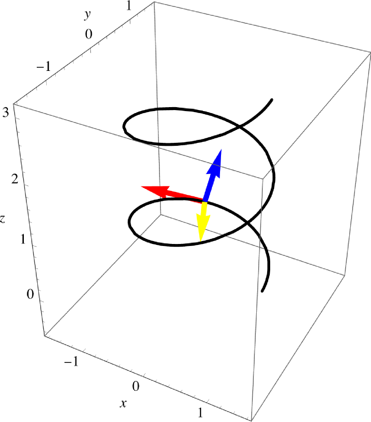
Figure 1: Helix ${\bf r}(s)$ (black), and ${\bf T}(s)$ (red), ${\bf N}(s)$ (yellow), ${\bf B}(s)$ (blue) plotted with parameters $r=1$ and $c=1/4$. The triad of unit vectors are plotted for $s=2$.

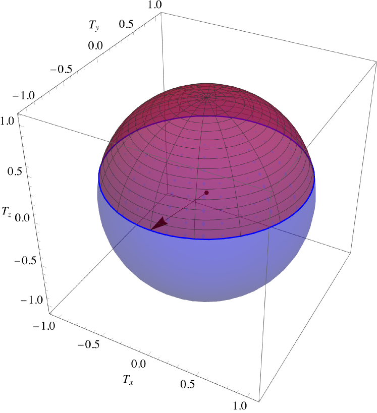
Figure 2: Tangent vector ${\bf T}$ on the Poincaré sphere plotted with parameters $r=1$ and $c=1/4$.

Figure 1 shows a helix ${\bf r}(s)$ with parameters $r=1$ and $c=1/4$ plotted in black, and the unit vectors ${\bf T}(s)$ (red), ${\bf N}(s)$ (yellow), ${\bf B}(s)$ (blue) evaluated at $s=2$. A triad of unit vectors can be plotted at any value of arc-length $s$.

Figure 2 shows the tangent vector ${\bf T}(s)$ on the unit sphere as a blue curve, where the unit vector ${\bf T}(s)$ goes from the origin to the blue curve. The solid angle on the sphere subtended by ${\bf T}(s)$ as $s$ moves from $s=0$ (see the black arrow from the origin of the sphere to the sphere surface) and back to this same point is colored red, but is semitransparent. We call this area $\Omega(r,c)$:

$$\Omega(r,c)=\frac{2\pi c}{\sqrt{r^{2}+c^{2}}}.$$ (15)

The figure was drawn for $r=1$ and $c=1/4$. As $r$ decreases (increases) the area decreases (increases), and as $c$ decreases (increases) the area increases (decreases).

IV Dynamics of light polarization in a helix fiber

For a fiber wound into a circular helix (e.g., by wrapping the fiber around a cylinder), an analytic solution for the polarization state of the light as a function of arc-length in a fiber with negligible birefringence is possible as both $r$ and $c$ are constants independent of $s$. The propagation equations for the polarization vector, which we call ${\bf A}(s)=A_{n}(s){\bf N}(s)+A_{b}(s){\bf B}(s)$, where the subscripts $n$ and $b$ stand for normal and binormal, is given by [6, 23]

$$i\,\frac{d}{ds}\left(\!\!\begin{array}[]{c}A_{n}(s)\\ A_{b}(s)\end{array}\!\!\right)=\left(\!\!\begin{array}[]{cc}-\frac{\alpha\,\kappa^{2}}{2}&i\tau\\ -i\tau&\frac{\alpha\,\kappa^{2}}{2}\end{array}\!\!\right)\left(\!\!\begin{array}[]{c}A_{n}(s)\\ A_{b}(s)\end{array}\!\!\right).$$ (16)

Here $\alpha$ is a constant given by the product of the radius of the optical fiber, $\rho$, and a constant depending on the wavelength of the light and the elastic material properties of the fiber, $a$, $\alpha=\rho a$ [6, 23]. With the most general initial conditions given by

$$A_{n}(0)=p,\qquad A_{b}(0)=e^{i\phi}\sqrt{1-p^{2}},$$ (17)

the solution to Eq. (16) takes the form,

$$A_{n}(s) = p\,\cos(\omega_{s}s)+\frac{2\tau e^{i\phi}\sqrt{1-p^{2}}+i\,\alpha\kappa^{2}p}{2\omega_{s}}\,\sin(\omega_{s}s),$$

$$A_{b}(s) = e^{i\phi}\sqrt{1-p^{2}}\cos(\omega_{s}s)$$ (18)

$$- \frac{2\tau p+i\,\alpha\kappa^{2}e^{i\phi}\sqrt{1-p^{2}}}{2\omega_{s}}\,\sin(\omega_{s}s),$$

where $\omega_{s}=\frac{1}{2}\sqrt{\alpha^{2}\kappa^{4}+4\tau^{2}}$.

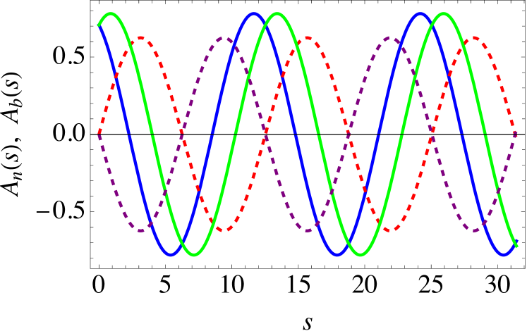
Figure 3: Amplitudes $A_{n}(s)$ and $A_{b}(s)$ of the normal and binormal vectors in the polarization vector ${\bf A}(s)$ for $p=1/\sqrt{2}$ and $\phi=0$ (linearly polarized light with polarization at a 45^∘ angle from the $x$-axis). Re$[A_{n}(s)]$ is the solid blue curve, Im$[A_{n}(s)]$ is the dashed red curve, Re$[A_{b}(s)]$ is the solid green curve, and Im$[A_{b}(s)]$ is the dashed purple curve.

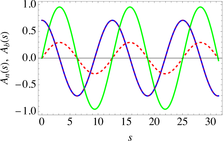
Figure 4: Amplitudes $A_{n}(s)$ and $A_{b}(s)$ of the normal and binormal vectors in the polarization vector ${\bf A}(s)$ for left circular polarized light, $p=1/\sqrt{2}$ and $\phi=\pi/2$. The Re$[A_{n}(s)]$ is the solid blue curve , Im$[A_{n}(s)]$ is the dashed red curve, Re$[A_{b}(s)]$ is the solid green curve, and Im$[A_{b}(s)]$ is the dashed purple curve which overlaps the solid blue Re$[A_{n}(s)]$ curve.

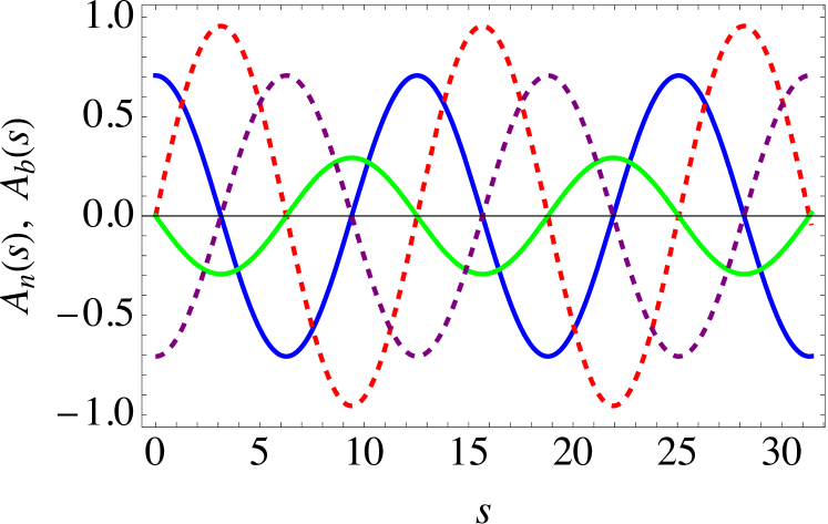
Figure 5: Amplitudes $A_{n}(s)$ and $A_{b}(s)$ of the normal and binormal vectors in the polarization vector ${\bf A}(s)$ for right circular polarized light, $p=1/\sqrt{2}$ and $\phi=-\pi/2$. The Re$[A_{n}(s)]$ is the solid blue curve, Im$[A_{n}(s)]$ is the dashed red curve, Re$[A_{b}(s)]$ is the solid green curve, and Im$[A_{b}(s)]$ is the dashed purple curve.

Figure 3 plots the amplitudes $A_{n}(s)$ and $A_{b}(s)$ versus $s$ for linearly polarized light with polarization at a 45^∘ angle from the $x$-axis, i.e., probability amplitude $p=1/\sqrt{2}$ and phase $\phi=0$. The parameter values used are $\alpha=1$, $r=1$ and $c=1/4$. The amplitudes have a period $T_{s}=2\pi/\omega_{s}=4\pi/\sqrt{\alpha^{2}\kappa^{4}+4\tau^{2}}$. The Im$[A_{n}(s)]$ and Im$[A_{b}(s)]$ curves are 180^∘ out of phase; Re$[A_{n}(s)]$ and Re$[A_{b}(s)]$ are out of phase by a much smaller angle.

Figure 4 plots the amplitudes $A_{n}(s)$ and $A_{b}(s)$ versus $s$ for left circular polarized light, i.e., probability amplitude $p=1/\sqrt{2}$ and phase $\phi=\pi/2$. In this case, Re$[A_{n}(s)]$ equals Im$[A_{b}(s)]$ so these curves lie one on top of the other. Figure 5 is somewhat similar to Fig. 4, except for right circular polarized light, $p=1/\sqrt{2}$ and $\phi=-\pi/2$, the Re$[A_{n}(s)]$ and Im$[A_{b}(s)]$ curves are distinct.

For understanding the physics of the polarization it is convenient to define the Stokes vector ${\bf S}(s)$ [24], which is a real vector that can be plotted on the Poincaré sphere (as can the complex polarization vector ${\bf A}(s)$ be plotted on the complex Bloch sphere [25]):

$${\bf S}(s) = \big{(}A_{n}^{*}(s),A_{b}^{*}(s)\big{)}\,\bm{\sigma}\,\left(\!\!\begin{array}[]{c}A_{n}(s)\\ A_{b}(s)\end{array}\!\!\right).$$ (21)

Here the Pauli vector is defined as $\bm{\sigma}=\sigma_{x}\hat{\bf x}+\sigma_{y}\hat{\bf y}+\sigma_{z}\hat{\bf z}$, and $\sigma_{x}$, $\sigma_{y}$ and $\sigma_{z}$ are the Pauli matrices. We now plot the Cartesian components of ${\bf S}(s)$ versus $s$ in Fig. 6 for the linearly polarized case where the amplitudes $A_{n}(s)$ and $A_{b}(s)$ are shown in Fig. 3. For this case the period of Stokes vector ${\bf S}(s)$ is half of the period $T_{S}$ of the amplitudes, where $T_{S}=12.5281$, as can be seen in all the figures for the amplitudes shown above.

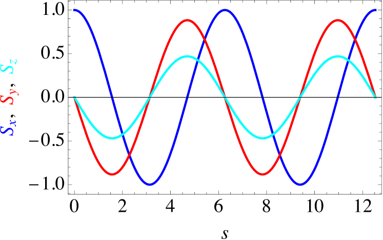
Figure 6: Polarization vector components of ${\bf S}(s)$ versus arc-length $s$ for initial conditions $p=1/\sqrt{2}$ and $\phi=0$ with with parameters $r=1$ and $c=1/4$.

Figure 7 shows the trajectory of the Stokes vector ${\bf S}(s)$ on the Poincaré sphere for $p=1/\sqrt{2}$ and $\phi=0$. The black arrow shows the polarization vector at $s=0$. As propagation proceeds, the tip of ${\bf S}(s)$ follows the red curve shown in the figure, making one full revolution at $s=T_{s}/2$ and two full revolutions at $s=T_{s}$. As the initial conditions change the solid angle subtended by ${\bf S}(s)$ on the Poincaré sphere changes; as $p$ increases from zero to one, the solid angle subtended increases. When $p=0$ and $p=1$, there is no dependence on $\phi$, but when $p\neq 0$, first the solid angle increases, then decreases, and it might again increase. The solid angle subtended equals the PBP, and more will be said about the PBP in Sec. V.

The position of the polarization vector on the Poincaré sphere can be quantified by the polar angle $\theta(s)$ and azimuthal angle $\phi(s)$. Figure 8 plots these angles versus $s$ for the linear polarization case with $p=1/\sqrt{2}$ and $\phi=0$. The discontinuities in $\phi(s)$ arises because of the way the azimuthal angle was calculated; it ranges from $-\pi$ to $\pi$. Clearly these angles are also periodic.

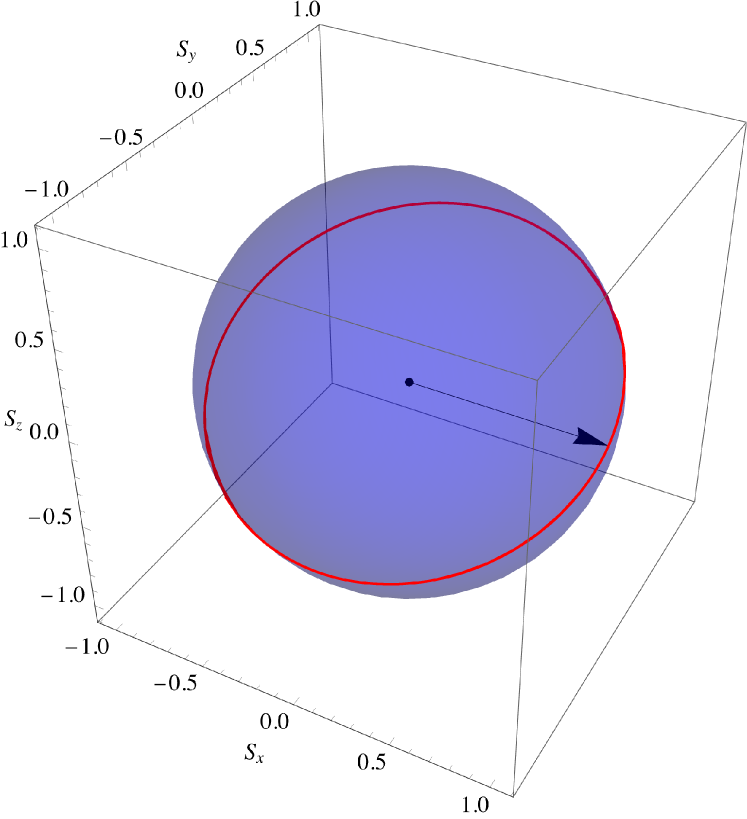
Figure 7: Polarization vector ${\bf S}$ plotted on the Poincaré sphere.

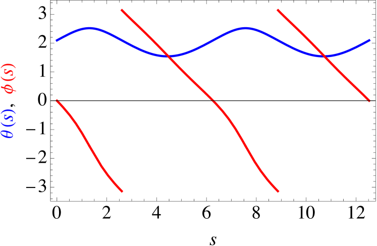
Figure 8: The polar and azimuthal angles of the polarization vector ${\bf S}(s)$, $\theta(s)$ and $\phi(s)$, versus $s$.

V Pancharatnam-Berry phase in a helix fiber

The geometrical phase can defined as follows [4, 17]:

$$\gamma_{B} = -i\int\limits_{0}^{T_{s}}\Big{(}A_{n}^{*}(s)\,\frac{dA_{n}(s)}{ds}+A_{b}^{*}(s)\,\frac{dA_{b}(s)}{ds}\Big{)}\,ds$$ (22)

$$= -\frac{2\pi[(1-2p^{2})\alpha\kappa^{2}-4p\sqrt{1-p^{2}}\,\tau\sin\phi]}{\sqrt{\alpha^{2}\kappa^{4}+4\tau^{2}}}.$$

Here $T_{s}=4\pi/\sqrt{\alpha^{2}\kappa^{4}+4\tau^{2}}$ is the period of the amplitudes $A_{n}(s)$ and $A_{b}(s)$ in Eq. (18).

In order to demonstrate that the PBP can be represented as a solid angle on the Poincaré sphere it is convenient to rewrite Eq. (16) as follows:

$$i\,\frac{d}{ds}\left(\!\!\begin{array}[]{c}A_{n}(s)\\ A_{b}(s)\end{array}\!\!\right)=\mathbb{B}\cdot\bm{\sigma}\,\left(\!\!\begin{array}[]{c}A_{n}(s)\\ A_{b}(s)\end{array}\!\!\right).$$ (23)

The $s$-independent vector $\mathbb{B}$ is given by

$$\mathbb{B}=-\tau\,\hat{\bf y}-\frac{1}{2}\,\alpha\kappa^{2}\,\hat{\bf z},$$

and its absolute value is $|\mathbb{B}|=2\pi/T_{s}$. Hence we can express $\gamma_{B}$ as

$$\gamma_{B}=-\frac{2\pi}{T_{s}}\int\limits_{0}^{T_{s}}\hat{\mathbb{B}}\cdot{\bf S}(s)\,ds,$$ (24)

where $\hat{\mathbb{B}}=\mathbb{B}/|\mathbb{B}|$ is the unit vector in the direction of $\mathbb{B}$, and the vector ${\bf S}(s)$ is defined in Eq. (21). It should be noted that the solution of Eq. (23) describes precession of the vector ${\bf S}(s)$ about the axis given by the unit vector $\hat{\mathbb{B}}$. Therefore, the projection of ${\bf S}(s)$ onto the precession axis, $\hat{\mathbb{B}}\cdot{\bf S}(s)$, does not depend on $s$ and is given by

$$\hat{\mathbb{B}}\cdot{\bf S}(s)=\frac{(1-2p^{2})\alpha\kappa^{2}-4p\sqrt{1-p^{2}}\,\tau\sin\phi}{\sqrt{\alpha^{2}\kappa^{4}+4\tau^{2}}}.$$ (25)

Substituting this equation into Eq. (24), we obtain Eq. (22).

Figure 9 plots the PBP $\gamma_{B}$ versus the probability amplitude $p$ and initial angle $\phi$ for parameters $r=1$ and $c=1/4$. $\gamma_{B}$ has a maximum of $\pi$ at $p=0.970339$ and $\phi=3\pi/2$, and a minimum of $-\pi$ at $p=0.241748$ and $\pi=\pi/2$. Note the symmetry of $\gamma_{B}$: making the transformation $p\to-p$ and $\phi\to-\phi$ (i.e., $\phi\to\phi+\pi$) leaves $\gamma_{B}$ unchanged, as is clear from Fig. 9.

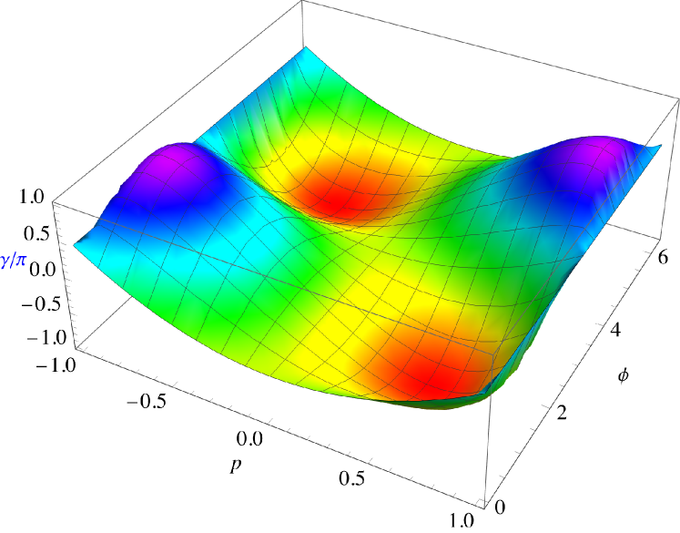
Figure 9: The PBP $\gamma_{B}$ (divided by $\pi$) versus the probability amplitude $p$ and initial angle $\phi$ for parameters $r=1$ and $c=1/4$. $\gamma_{B}/\pi$ ranges from -1 and 1.

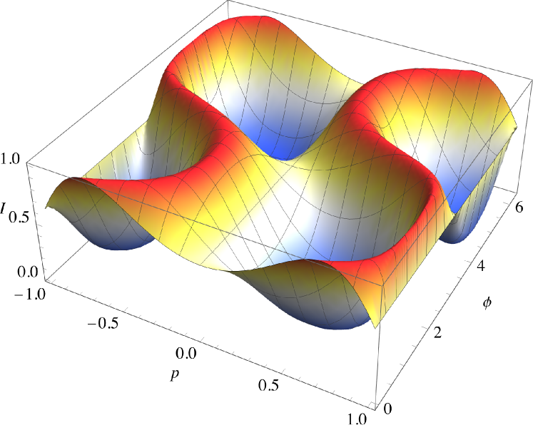
Figure 10: Intensity $I$ plotted as a function of the initial conditions $p$ and $\phi$ that is obtained upon taking a coherent superposition of a fraction of the incident beam at $s=0$ and the same fraction of the beam at $s=T_{s}$.

Figure 10 plots the intensity $I$ obtained upon taking a coherent superposition of a fraction of the incident beam at $s=0$ and the same fraction of the beam at $s=T_{s}$. The intensity is proportional to $\cos^{2}(\gamma_{B}/2)=(1+\cos\gamma_{B})/2$, which ranges from 0 to 1. Note that $s=T_{s}$ is not the arc-length at which the helix tangent vector returns to its initial value ${\bf T}(0)$. This is clear from Eq. (4); the period for the tangent vector returning to its original position is $2\pi\sqrt{r^{2}+c^{2}}=\tfrac{2\pi}{\sqrt{\kappa^{2}+\tau^{2}}}\neq T_{s}=\tfrac{4\pi}{\sqrt{\alpha^{2}\kappa^{4}+4\tau^{2}}}$.

V.1 Relationship between $\gamma_{B}$ and $\Omega$

Here we compare the solid angle $\Omega(r,c)$ given in Eq. (15) and the PBP $\gamma_{B}$ given in Eq. (22). Note that $\gamma_{B}$ depends on the initial conditions parameterized by $p$ and $\phi$, see Eq. (17), and the parameter $\alpha$ (which depends on the fiber radius and elastic properties of the material). In contradistinction, $\Omega(r,c)$ is a function only of the helix radius $r$ and pitch $2\pi c$ (it does not depend upon $\alpha$, nor on the initial conditions). Solving Eqs. (5) and (8) for $r$ and $c$ in terms of $\kappa$ and $\tau$, we get $r=\frac{\kappa}{\kappa^{2}+\tau^{2}}$, $c=\frac{\tau}{\kappa^{2}+\tau^{2}}$, and substituting these equations into Eq. (15), we can express $\Omega(\kappa,\tau)$ as a function of the curvature $\kappa$ and the torsion $\tau$:

$$\Omega(\kappa,\tau)=\frac{2\pi\tau}{\sqrt{\kappa^{2}+\tau^{2}}}.$$ (26)

Comparing Eqs. (26) and (22) reveals that

$$\gamma_{B}=\pm\,\Omega(\kappa,\tau),$$ (27)

provided that

1. $\alpha=2/\kappa$ (which is very improbable given that $\alpha$ depends on the material characteristics of the fiber),

2. the light is circularly polarized: $p=\tfrac{1}{\sqrt{2}}$, $\phi=\pm\tfrac{\pi}{2}$.

Unfortunately, Eq. (27) is frequently cited in the literature without specifying these provisions, e.g., see Refs. [2, 26, 13].

VI Fluctuations of the PBP due to fluctuations of the helix parameters

Let us now examine the fluctuations of $\gamma_{B}(\kappa,\tau,\alpha)$ as a result of possible fluctuations in the fiber parameters $r$, $c$ and $\alpha$. For example, let us assume that there is a Gaussian probability distribution for some of the parameters $r$, $c$ and $\alpha$, with expectation values designated as $r_{0}$, $c_{0}$ and $\alpha_{0}$, and the variances $\sigma_{r}^{2}$, $\sigma_{c}^{2}$ and $\sigma_{\alpha}^{2}$. Assuming that the standard deviations of the variables are smaller than the corresponding mean values, $\sigma_{r}\ll r_{0}$, $\sigma_{c}\ll c_{0}$ and $\sigma_{\alpha}\ll\alpha_{0}$, and neglecting terms of order $\sigma^{4}$, we find the expectation value $\bar{\gamma}_{B}$ of $\gamma_{B}(\kappa,\tau,\alpha)$ and its variance $\sigma_{\gamma_{B}}^{2}$:

$$\bar{\gamma}_{B} = \gamma_{B}(r_{0},c_{0},\alpha_{0})+\frac{\partial^{2}\gamma_{B}(r_{0},c_{0},\alpha_{0})}{\partial r_{0}^{2}}\sigma_{r}^{2}$$ (28)

$$+ \frac{\partial^{2}\gamma_{B}(r_{0},c_{0},\alpha_{0})}{\partial c_{0}^{2}}\sigma_{c}^{2}+\frac{\partial^{2}\gamma_{B}(r_{0},c_{0},\alpha_{0})}{\partial\alpha_{0}^{2}}\sigma_{\alpha}^{2},\quad$$

$$\sigma_{\gamma_{B}}^{2} = \bigg{(}\frac{\partial\gamma_{B}(r_{0},c_{0},\alpha_{0})}{\partial\ln r_{0}}\bigg{)}^{2}\frac{\sigma_{r}^{2}}{r_{0}^{2}}+\bigg{(}\frac{\partial\gamma_{B}(r_{0},c_{0},\alpha_{0})}{\partial\ln c_{0}}\bigg{)}^{2}\frac{\sigma_{\tau}^{2}}{\tau_{0}^{2}}$$ (29)

$$+ \bigg{(}\frac{\partial\gamma_{B}(\kappa_{0},\tau_{0},\alpha_{0})}{\partial\ln\alpha_{0}}\bigg{)}^{2}\frac{\sigma_{\alpha}^{2}}{\alpha_{0}^{2}}.$$

Let us consider two special cases. (a) For linearly polarized light with $p=1$, we find

$$\bar{\gamma}_{B} = \frac{2\pi\alpha_{0}r_{0}^{2}}{\sqrt{c_{0}^{2}(r_{0}^{2}+c_{0}^{2})^{2}+\alpha_{0}^{2}r_{0}^{4}}}+\frac{2\pi\alpha_{0}r_{0}^{2}c_{0}^{2}}{(c_{0}^{2}(r_{0}^{2}+c_{0}^{2})^{2}+\alpha_{0}^{2}r_{0}^{4})^{5/2}}$$ (30)

$$\times\bigg{\{}\frac{2\sigma_{r}^{2}}{r_{0}^{2}}\,c_{0}^{2}\,\Big{[}c_{0}^{2}\big{(}r_{0}^{2}+c_{0}^{2}\big{)}^{2}\big{(}c_{0}^{2}-3r_{0}^{2}\big{)}$$

$$-\alpha_{0}^{2}r_{0}^{4}\big{(}3r_{0}^{4}+5c_{0}^{2}\big{)}\Big{]}$$

$$+\frac{\sigma_{c}^{2}}{c_{0}^{2}}\Big{[}2c_{0}^{2}\big{(}r_{0}^{2}+c_{0}^{2}\big{)}^{2}\big{(}r_{0}^{4}+3r_{0}^{2}c_{0}^{2}+6c_{0}^{4}\big{)}$$

$$-\alpha_{0}^{2}r_{0}^{4}\big{(}r_{0}^{4}+12r_{0}^{2}c_{0}^{2}+15c_{0}^{4}\big{)}\Big{]}$$

$$-3\sigma_{\alpha}^{2}\,r_{0}^{4}\big{(}r_{0}^{2}+c_{0}^{2}\big{)}^{2}\bigg{\}},$$

$$\sigma_{\gamma_{B}}^{2} = \frac{4\pi^{2}\alpha_{0}^{2}r_{0}^{4}c_{0}^{4}(r_{0}^{2}+c_{0}^{2})^{2}}{(c_{0}^{2}(r_{0}^{2}+c_{0}^{2})^{2}+\alpha_{0}^{2}r_{0}^{4})^{3}}\bigg{(}\frac{4c_{0}^{4}\sigma_{r}^{2}}{r_{0}^{2}}+\frac{(r_{0}^{2}+3bc_{0}^{2})^{2}\sigma_{c}^{2}}{c_{0}^{2}}$$ (31)

$$+\frac{(r_{0}^{2}+c_{0}^{2})^{2}\sigma_{\alpha}^{2}}{\alpha_{0}^{2}}\bigg{)}.$$

(b) For circularly polarized light with $p=1/\sqrt{2}$ and $\phi=\pi/2$,

$$\bar{\gamma}_{B} = \frac{4\pi c_{0}(r_{0}^{2}+c_{0}^{2})}{\sqrt{c_{0}^{2}(r_{0}^{2}+c_{0}^{2})^{2}+\alpha_{0}^{2}r_{0}^{4}}}+\frac{4\pi\alpha_{0}^{2}r_{0}^{4}c^{3}_{0}}{(c_{0}^{2}(r_{0}^{2}+c_{0}^{2})^{2}+\alpha_{0}^{2}r_{0}^{4})^{5/2}}$$ (32)

$$\times \bigg{\{}6\frac{\sigma_{r}^{2}}{r_{0}^{2}}\,\big{[}\alpha_{0}^{2}r_{0}^{4}+r_{0}^{4}c_{0}^{2}-c_{0}^{6}\big{]}$$

$$-3\frac{\sigma_{c}^{2}}{c_{0}^{2}}\,\big{[}r_{0}^{6}-2\alpha_{0}^{2}r_{0}^{4}+3r_{0}^{4}c_{0}^{2}+11r_{0}^{2}c_{0}^{4}+7c_{0}^{6}\big{]}$$

$$-\frac{\sigma_{\alpha}^{2}}{\alpha_{0}^{2}}\,\frac{r_{0}^{2}+c_{0}^{2}}{c_{0}^{2}}\,\big{[}c_{0}^{2}(r_{0}^{2}+c_{0}^{2})^{2}-2\alpha_{0}^{2}r_{0}^{4}\big{]}\bigg{\}},$$

$$\sigma_{\gamma_{B}}^{2} = \frac{4\pi^{2}\alpha_{0}^{2}r_{0}^{4}c_{0}^{4}(r_{0}^{2}+c_{0}^{2})^{2}}{(c_{0}^{2}(r_{0}^{2}+c_{0}^{2})^{2}+\alpha_{0}^{2}r_{0}^{4})^{3}}\,\bigg{(}4c_{0}^{4}\frac{\sigma_{r}^{2}}{r_{0}^{2}}+(r_{0}^{2}+3c_{0}^{2})^{2}\frac{\sigma_{c}^{2}}{c_{0}^{2}}$$ (33)

$$+(r_{0}^{2}+c_{0}^{2})^{2}\frac{\sigma_{\alpha}^{2}}{\alpha_{0}^{2}}\bigg{)}.$$

Note that the expectation value $\bar{\gamma}_{B}$ depends on the variances of $r$, $c$, and $\alpha$ i.e., $\bar{\gamma}_{B}\neq\gamma_{B}(r_{0},c_{0},\alpha_{0})$. Hence, average experimental results depend on the variances.

VII Summary and Conclusions

The concept of geometric phase is fundamental and establishes a deep connection between classical mechanics, quantum mechanics and optics (where it is referred to as the PBP $\gamma_{B}$). In this work, we have analyzed the geometric phase $\gamma_{B}$ for light propagating in a circular helix optical fiber. Using the Frenet-Serret system, the curvature $\kappa$, the torsion $\tau$, and the three orthogonal vectors, the tangent vector ${\bf T}$, the normal vector ${\bf N}$, and the binormal vector ${\bf B}$ along the helical curve are obtained. An analytic expression for the amplitudes $A_{n}(s)$ and $A_{b}(s)$ in the polarization vector ${\bf A}(s)=A_{n}(s){\bf N}(s)+A_{b}(s){\bf B}(s)$ as a function of the arc-length $s$, and the PRB $\gamma_{B}$ for arbitrary initial conditions of the polarization are derived in Secs. IV and V, respectively. Section V.1 shows that, even for circularly polarized light, $\gamma_{B}$ is not equal to the solid angle $\Omega(r,c)$ on the sphere subtended by ${\bf T}(s)$ as $s$ moves from $s=0$ and back to the same point. $\gamma_{B}$ depends on the parameter $\alpha=\rho a$, which is the product of the radius of the optical fiber, $\rho$, and a constant $a$ which depends on the wavelength of the light and the elastic properties of the fiber. In contrast, $\Omega(r,c)$ is not dependent on $a$. The dependence of the mean and standard deviation of the PBP $\gamma_{B}$ on fluctuations of the parameters $r,c,\alpha$ is discussed in Sec. VI. The expectation value of $\gamma_{B}$ is dependent upon the variances of $r$, $c$, and $\alpha$. Although it is well established that disorder can result in the localization of light, as evidenced by previous research [27, 28], a comprehensive understanding of the impact of disorder on light polarization and the PBP remains a topic for further investigation.

References

- [1] S. Pancharatnam, “Generalized theory of interference, and its applications. Part I.”, Proc.Ind. Acad. Sci. A44, 247 (1956).
- [2] M. J. Berry, “The adiabatic phase and Pancharatnam’s phase for polarized light”, J. Mod. Optics 34, 1401 (1987).
- [3] D. J. Sorce and S. Michaeli, “On the geometric phases during radio frequency pulses with sine and cosine amplitude and frequency modulation”, AIP Advances 13, 085210 (2023).
- [4] M. V. Berry, “Quantal phase factors accompanying adiabatic changes”, Proc. R. Soc., Lond. A392, 45 (1984).
- [5] B. Simon, “Holonomy, the Quantum Adiabatic Theorem, and Berry’s Phase”, Phys. Rev. Lett. 51, 2167 (1983).
- [6] J. N. Ross, “The rotation of the polarization in low birefringence monomode optical fibers due to geometric effects”, Optical and Quantum Electronics 16, 455 (1984).
- [7] C. P. Jisha, S. Nolte, and A. Alberucci, “Geometric Phase in Optics: From Wavefront Manipulation to Waveguiding”, Laser Photonics Rev. 2100003, 15 (2021).
- [8] J. Wang, et al. “Experimental observation of Berry phases in optical Möbius-strip microcavities” Nature Photonics 17, 120 (2023).
- [9] T. B. Mieling, M. A. Oancea, “Polarization transport in optical fibers beyond Rytov’s law”, Phys. Rev. Research 5, 023140 (2023).
- [10] Z. Bomzon, G. Biener, V. Kleiner, E. Hasman, “Space-variant Pancharatnam-Berry phase optical elements with computer-generated subwavelength gratings”, Opt. Lett. 27, 1141 (2002).
- [11] E. Hasman, V. Kleiner, G. Biener, A. Niv, “Polarization Dependent Focusing Lens by Use of Quantized Pancharatnam-Berry Phase Diffractive Optics”, Appl.Phys.Lett. 82, 328 (2003).
- [12] L. Marrucci, C. Manzo, D. Paparo, “Optical Spin-to-Orbital Angular Momentum Conversion in Inhomogeneous Anisotropic Media”, Phys. Rev. Lett. 96, 96, 163905 (2006).
- [13] A. Tornita, R. Y. Chiao, “Observation of Berry’s Topological Phase by Use of an Optical Fiber”, Phys. Rev. Lett. 57, 937 (1986).
- [14] T. T. Wu and C. N. Wang, “Concept of nonintegrable phase factors and global formulation of gauge fields”, Phys. Rev. D12, 3845, 1975.
- [15] A. Hannonen, H. Partanen, A. Leinonen, J. Heikkinen, T. K. Hakala, A. T. Friberg, T. Setä, “Measurement of the Pancharatnam-Berry phase in two-beam interference”, Optica 7, 1435 (2020).
- [16] M. F. Ferrer-Garcia, K. Snizhko, A. D’Errico1, A. Romito, Y. Gefen, E. Karimi, “Topological transitions of the generalized Pancharatnam-Berry phase”, Sci. Adv. 9,6810 (2023).
- [17] J. C. Solem and L. C. Biedenharn, “Understanding Geometrical Phases in Quantum Mechanics: An Elementary Example”, Foundations of Physics 3,, 185 (1993).
- [18] H. C. Longuet Higgins, U. Öpik, M. H. L. Pryce, R. A. Sack “Studies of the Jahn-Teller effect. II. The dynamical problem”, Proc. R. Soc. A. 244, 1, (1958).
- [19] Y. Aharonov, D. Bohm, “Significance of electromagnetic potentials in quantum theory”, Physical Review. 115, 485 (1959).
- [20] F. Wilczek, A. Shapere, Eds., Geometric Phases in Physics, (World Scientific, Singapore, 1989), pp. 3-4.
- [21] D. Suter, K. T. Mueller and A. Pines, “Study of the Aharonov-Anandan Quantum Phase by NMR Interferometry”, Ibid., p. 221.
- [22] https://en.wikipedia.org/wiki/Frenet%E2%80%93Serret_formulas.
- [23] R.C. Jones, “A New Calculus for the Treatment of Optical Systems. VII. Properties of the N-Matrices”, J. Opt. Soc. Amer. 38 671 (1948).
- [24] J. D. Jackson, Classical Electrodynamics, 3rd Ed., (John Wiley & Sons, Hoboken, 1999), section 7.2.
- [25] Y. B. Band, Light and Matter: Electromagnetism, Optics, Spectroscopy and Lasers, Chapter 1, (J. Wiley, NY, 2006)
- [26] R. Y. Chiao, Y-S Wu, “Manifestations of Berry’s Topological Phase for the Photon”, Phys. Rev. Lett. 57, 933 (1986).
- [27] D. S. Wiersma, P. Bartolini, A. Lagendijk, R. Righini, “Localization of light in a disordered medium”, Nature 390, 671 (1997).
- [28] M. Segev, Y. Silberberg and D. N. Christodoulides, “Anderson localization of light”, Nature Photonics 7, 197 (2013).