Complete Security and Privacy for AI
Inference in Decentralized Systems

Abstract

The need for data security and model integrity has been accentuated by the rapid adoption of AI and ML in data-driven domains including healthcare, finance, and security. Large models are crucial for tasks like diagnosing diseases and forecasting finances but tend to be delicate and not very scalable. Decentralized systems solve this issue by distributing the workload and reducing central points of failure. Yet, data and processes spread across different nodes can be at risk of unauthorized access, especially when they involve sensitive information. Nesa solves these challenges with a comprehensive framework using multiple techniques to protect data and model outputs. This includes zero-knowledge proofs for secure model verification. The framework also introduces consensus-based verification checks for consistent outputs across nodes and confirms model integrity. Split Learning divides models into segments processed by different nodes for data privacy by preventing full data access at any single point. For hardware-based security, trusted execution environments are used to protect data and computations within secure zones. Nesa’s state-of-the-art proofs and principles demonstrate the framework’s effectiveness, making it a promising approach for securely democratizing artificial intelligence.

1 Introduction

Artificial Intelligence (AI), particularly machine learning (ML), has made significant strides in recent decades. Since the advent of large language models (LLMs) such as ChatGPT [1], Claude [2], Gemini [3], LLaMA [4] and diffusion models [5] such as DALLE-3 [6] and Sora [7], foundation models have garnered considerable attention. While these foundation models exhibit intriguing properties such as in-context learning and chain-of-thought reasoning, concerns about their security and privacy have emerged, especially in distributed or decentralized computing scenarios. For instance, in ML as a service (MLaaS), ensuring the integrity of inference results is paramount. Service providers must demonstrate to customers that the output stems from inputting the customer’s prompt into a verified large language model, like GPT-4, and generating the response through model execution, rather than relying on human writers or less advanced models, such as GPT-3.5. This requirement is referred to as model security or model integrity. Meanwhile [8], service providers are reluctant to release their model weights, preferring to keep them confidential. In distributed or decentralized inference applications, a central server divides a foundation model into distinct segments, each managed by a different party. When an inference query arises, each party executes its segment independently. It is key to ascertain the trustworthiness of each party’s execution before aggregating the outputs.

Meanwhile, data privacy issues also arise in decentralized inference [9], where users need to ensure that their input data are not directly visible to the decentralized nodes that carry the AI inference for them. This can be extremely important in “critical inference” settings where sensitive information, such as medical records, financial data, or security information, is processed. In healthcare, where AI models analyze medical images like MRI or CT scans to diagnose diseases. Patient data is highly sensitive and must be protected. Ensuring data privacy in such scenarios is crucial to protect user data from unauthorized access and potential misuse.

At Nesa, we aim to address security and privacy concerns for AI’s responsible and effective deployment across various domains. In a nutshell, we design hybrid approaches to security and privacy [10] for the above challenges. The selection of different security and privacy methods depends on the specific use cases and the need for varying levels of security and privacy. Based on the different levels of needs, users can flexibly choose the best option for security and privacy. Here, we discuss two key scenarios at Nesa and our security and privacy approaches to them. Also, we discuss how we adapt a hardware-based trusted execution environment (TEE) as an orthogonal approach for security and privacy.

Scenario 1: Critical inference refers to scenarios where the results of AI inference are extremely significant, necessitating the highest levels of security and privacy, even if it means slower speed and higher cost. In these situations, the accuracy and confidentiality of the inference outcomes are important, and users are willing to endure longer processing times to ensure their data is fully protected. Examples include healthcare diagnostics, where AI analyzes medical images to detect diseases, and financial decision-making, where AI evaluates large transactions or investment strategies. In both cases, the sensitive nature of the data demands robust privacy measures, with stakeholders prioritizing data security over rapid results to prevent unauthorized access and ensure the integrity of the process. Under this scenario, Nesa adapts and innovates two leading technologies, including zero-knowledge machine learning (ZKML) [11] for model integrity verification and homomorphic encryption (HE) for data encryption and user privacy protection. Admittedly, the original design of ZKML and HE is computationally heavy, especially for non-linear layers in neural networks such as ReLU layers [12]. To balance effectiveness and efficiency, we apply the state-of-the-art ZKML techniques introduced by [11, 13] to build zero-knowledge Decentralized Proof System (zkDPS) for proof generation and verification processes in foundation models, and we apply HE selectively to critical layers rather than the entire model. Specifically, we propose Sequential Vector Encryption (SVE) based on sequential homomorphic encryption (SHE). This robust encryption scheme obfuscates the output of each operator in a neural network to prevent attackers from extracting sensitive information from intermediate representations. §2 provides more details on our customized zkDPS and SHE solutions for critical inference with the highest protection.

Scenario 2: General inference refers to everyday AI inference tasks with less critical results, allowing for faster processing speeds and lower costs without compromising basic security and privacy standards. In these scenarios, a certain level of protection is still necessary, but the stringent measures required for critical inference are not needed. Examples include routine tasks such as checking the weather, recommending products, or filtering spam emails. Here, the emphasis is on efficiency and speed while maintaining adequate data security to protect user information. Under this scenario, Nesa employs our consensus-based verification (CBV) for security, ensuring the integrity of the inference process, and split learning (SL) [14] for data encryption, which provides a reasonable level of data protection. Notably, we have innovated this verification method to reduce the high redundancy requirements in model verification, and split learning has been used in decentralized AI encryption for the first time. §3 elaborates on our consensus-based verification and split learning solutions for general inference, balancing speed and security effectively.

NTEE: Nesa’s Trusted Execution Environment (TEE). In addition to our innovations around software- and/or algorithm-based security and privacy approaches for the two scenarios, we also design an orthogonal hardware-based approach for both. In a nutshell, TEEs create secure isolation zones within the network’s nodes, protecting user data and private model parameters from unauthorized access [15]. TEEs provide a secure enclave for executing computations, isolated from the rest of the node’s operating environment, ensuring that even if other parts of the node are compromised, the computations within the TEE remain protected. This isolation is critical in decentralized settings where AI models are spread among multiple owners. This hardware-based security measure works as an alternative to algorithm-based approaches, providing a fast and efficient solution for Nesa’s decentralized AI inference tasks. Additionally, we innovate NTEE (Nesa TEEs) optimizing communication among multiple TEEs by establishing direct, secure channels, and implementing heterogeneous TEE scheduling based on the capabilities of each node, whether CPU or GPU-based. NTEE facilitates secure collaboration across multiple nodes, enabling Nesa to maintain high performance, robust security, and data privacy, making it ideal for both critical and general inference scenarios. See details of our TEE implementation and innovation in §4.

Table 1: Summary of our proposed security and privacy solutions.

Type	Scenario	Solution to Model Verification	Solution to User Privacy
Algorithm	Critical (§2)	zero-knowledge Decentralized Proof System (zkDPS) (§2.1)	Sequential Vector Encryption (SVE) (§2.2)
Algorithm	General (§3)	Consensus-Based Verification (CBV) (§3.1)	Split Learning (SL) (§3.2)
Hardware	Both	TEE model verification (§4)	TEE secure channel (§4)

Table 1: Summary of Security and Privacy Solutions (continued)

Choosing Security and Privacy Options. Table LABEL:table:suecurity-all summarizes our innovations around security and privacy. Here, we further discuss the choice of different methods by scenario. Given critical inference scenarios, where the final results have high value and users are willing to wait longer, we suggest using zkDPS for model verification and SHE for data encryption. In contrast, for general inference scenarios, where the results are less critical and faster processing is desired, we recommend using CBV for model verification and SL for data encryption. Additionally, the TEE-based solution, NTEE, can also be leveraged as an orthogonal approach. Once NTEE is employed, it addresses both verification and encryption needs simultaneously. However, it is important to note that GPU TEEs are only available on high-end GPUs, making the trade-off such that TEE solutions are mostly CPU-based. In contrast, algorithm-based solutions can fully leverage GPUs, offering a different balance of performance and security. This approach allows us to balance the trade-offs between security, privacy, and efficiency, ensuring that users can select the most appropriate solution for their specific needs. By leveraging both algorithm-based and hardware-based security measures, Nesa can provide robust and adaptable security and privacy solutions across a wide range of AI applications. This adaptive approach ensures that users can select the most appropriate level of protection for their data and applications, achieving an optimal balance among security, privacy, and performance.

2 Security and Privacy for Critical Inference

Figure 1: Security flowchart for critical inference, where Nesa designs zkDPS (§2.1) for model verification and SHE (§2.2) for data encryption and user privacy protection.

In critical inference scenarios, the significance of AI inference results necessitates the highest levels of security and privacy, as the outcomes directly impact crucial sectors like healthcare and finance. Our strategy for ensuring model verification and integrity is via our Zero-Knowledge Decentralized Proof System (zkDPS), a specialized ZK system for decentralized LLMs that allows one party to prove to another that a statement is true without revealing any information beyond the validity of the statement itself. Notably, it introduces a few new techniques to speed up the ZK process. This approach is detailed in §2.1. For data privacy, we redesign Sequential Homomorphic Encryption (SHE) and propose our Sequential Vector Encryption (SVE), which enables computations on encrypted data without decrypting it, thus ensuring that sensitive data remains protected throughout the inference process. In comparison to classical HE, our approaches can be more efficient in applying implied tensor transformations to selected layers of an AI model. More information on this technique can be found in Section 2.2. Fig. 1 summarizes the security flow of critical inference at Nesa, where the data will be transmitted with SVE for encryption, and the final inference results will be verified by zkDPS for integrity.

2.1 Zero-Knowledge Machine Learning for Model Integrity

2.1.1 Background

Despite the significant strides made in AI security in recent years, the potency of attacks has surged. Central to AI security is the pivotal task of delineating the threat model and understanding how adversaries target the inference process. Adversaries can exploit various vulnerabilities within the inference systems of foundational models, employing tactics tailored to different scenarios. In decentralized AI inference environments, one threat model emerges, where computing nodes may behave deceitfully, compromising the integrity of aggregated results. It becomes imperative to establish mechanisms wherein each node can verify its adherence to agreed-upon protocols without compromising the confidentiality of its model. This necessitates enabling nodes to provide proofs of honest execution to the central server or the public while safeguarding the confidentiality of their respective models. Thus, ensuring both the integrity of inference processes and the privacy of model architectures becomes paramount in the realm of AI security.

In the realm of defending against adversarial attacks, a plethora of meticulously crafted countermeasures exist to safeguard systems. One such strategy, particularly pertinent in decentralized inference settings, involves the implementation of mechanisms where central servers solicit proof of computing execution from each node. This process is orchestrated with precision to ensure that while the proof is furnished, the node’s confidential model parameters remain undisclosed. Subsequently, the central servers meticulously scrutinize the proofs submitted, thereby enabling them to discern the reliability of each node. The efficacy of this approach hinges upon the successful verification of the proof, serving as a litmus test for the trustworthiness of the node in question.

The challenge intensifies when fast inference of secure foundation models is required. Given the scale of big data and the models involved, foundation models inherently exhibit slow inference speeds. It is widely acknowledged that incorporating security measures further exacerbates this slowdown in AI models. For instance, the fastest-known zero-knowledge proof algorithm currently takes as long as 15 minutes to generate proof for a single token in the output [13]. Despite substantial efforts to expedite the inference process, it is imperative to ensure the security of foundation model inference without compromising efficiency.

2.1.2 Problem Setups

Decentralized Inference. At Nesa, we explore the challenge of decentralized inference for foundation models, which offers numerous benefits. With the advent of 5G technology and improved internet latency, personalized devices such as mobile phones can now participate in crowdsourcing machine learning models. This approach enhances device utilization and eliminates the need for data communication between nodes and a central server, thereby safeguarding data privacy. In the context of Machine Learning as a Service (MLaaS), models remain the private property of individual nodes, allowing them to offer model inference services via APIs without sharing model weights and checkpoints. As foundation models grow in size—such as Meta’s LLaMA-3.1 with 405 billion parameters [4], and future models expected to reach trillion-level sizes—it becomes impractical to load entire models on a single node or server. Additionally, technologies like blockchain are now equipped to support the decentralized inference of foundation models on-chain, further facilitating this approach.

Model Decomposition. A core assumption in decentralized AI inference is that the model used in the inference system can be divided into several parts, each managed by a separate party, or computing node. Each computing node performs its assigned computations and sends the results to a central server. For instance, with a foundation model like LLaMA-3, the model can be decomposed layer-wise, enabling sequential inference by different nodes. Alternatively, decomposing the model width-wise allows for parallel inference across multiple nodes. The method of decomposition depends entirely on the application scenarios, and we consider both approaches in Nesa’s products.

2.1.3 Threat Models

In this paper, we focus on decentralized inference of foundation models as described above. In this framework, each computing node (i.e. prover) owns a foundation model or a part of the foundation model with a publicly known architecture, while the model weights are proprietary. We make a semi-dishonest assumption on the central server (i.e. verifier): the central server is honest in aggregating results from each computing node and accurately reports the verification result, but the central server tries to glean additional information about parts of the foundation model at computing nodes. However, some computing nodes might be dishonest, potentially deviating from the agreed protocol by substituting their model with an alternative or outputting random data. We assume that the majority of nodes are honest, but acknowledge that dishonest nodes can collude. These adversarial nodes can arbitrarily alter their results, provided their behavior remains undetected by the central server.

2.1.4 Overview of Zero-Knowledge Proofs

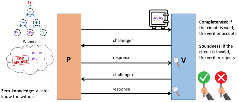
Figure 2: Zero-knowledge proof of circuit $10=(w_{1}+w_{2})(w_{2}+1)$ between a prover (P) and a verifier (V). Hereby, the goal of the prover is to prove to the verifier that P knows a $w_{1}$ and $w_{2}$ such that the claimed result “10” is indeed calculated by the equation $(w_{1}+w_{2})(w_{2}+1)$ (which is denoted by a circuit). The witness $w_{1}=4$ and $w_{2}=1$ are the secret of the prover. Zero-knowledge proof consists of a commitment process (denoted by the safe box) in the beginning, followed by several back-and-forth challenge and response processes between P and V in the interactive scenario. In the non-interactive scenario, the prover can challenge him or herself by the Fiat-Shamir heuristic and the verifier only needs to verify the last response from the prover.

We use the technique of zero-knowledge proofs to guarantee that each party is honest about his or her execution of inference of foundation models. Zero-knowledge proof serves as a fundamental technique and underpins the architecture of blockchain. In this cryptographic concept, two entities are involved: the prover and the verifier. The prover’s objective is to demonstrate the successful execution of a protocol without disclosing confidential information, termed as the ’witness’. This witness encompasses sensitive data like model weights or private information that the prover wishes to keep undisclosed to the verifier. Often, the protocol is depicted as a circuit, where certain components remain hidden within the witness.

Commitment, Proof, and Verification. The process of zero-knowledge proof involves three essential steps. Firstly, the prover commits to the witness data, such as model parameters, ensuring its integrity by encrypting it before transmitting it to the verifier. Once sent, the content remains unchanged, with the verifier gaining access only to the encrypted version. In practice, the (generalized Pedersen) commitment of any $d$-dimensional tensor $\textbf{S}=(S_{1},S_{1},...,S_{d})\in\{0,1,...,|\mathbb{G}|-1\}^{d}$ (e.g., the model weights) is implemented as [16]:

$$\textsf{Commit}(\textbf{S},r_{S})=h^{r_{S}}\textbf{g}^{\textbf{S}}=h^{r_{S}}\prod_{i=1}^{d}g_{i}^{S_{i}},$$ (1)

where $\mathbb{G}$ is an elliptic curve group w.r.t. the finite field $\mathbb{F}$ consisting of points $(x,y)\in\mathbb{F}\times\mathbb{F}$ such that $y^{2}=x^{3}+ax+b$ for designated field elements $a$ and $b$, $r\sim\{0,1,...,|\mathbb{G}|-1\}$ is an integer (i.e., the element of the scalar field $\mathbb{F}$ of $\mathbb{G}$ with $|\mathbb{F}|=|\mathbb{G}|$) uniformly sampled from $\{0,1,...,|\mathbb{G}|-1\}$, $\textbf{g}=(g_{1},g_{2},...,g_{d})\in\mathbb{G}^{d}$ and $h\sim\mathbb{G}$ are uniformly and independently sampled from $\mathbb{G}$. In the second step, the prover executes the protocol and simultaneously generates a proof of execution in a finite field $\mathbb{F}$, which is then transmitted to the verifier, either interactively or non-interactively. Depending on the protocol, operations can involve arithmetic or non-arithmetic processes. Lastly, the verifier meticulously examines the proof to ensure the honest execution of the protocol by the prover, thereby validating the transaction or information under scrutiny.

2.1.5 Properties of Zero-Knowledge Proofs

Zero-knowledge proofs have many advantageous properties that form the foundation of blockchain and decentralized machine learning. These include:

Completeness: If the prover accurately executes the circuit, the proof will be validated (with probability 1).

Special Soundness: If the prover is dishonest in executing the circuit, the proof will fail (with high probability). A weaker property, special soundness, requires executing the protocol twice and being able to identify the witness.

Zero-Knowledge: The verifier gains no knowledge about the prover’s witness.

The above properties ensure that the proof will pass verification only if the prover is honest, while also allowing the prover to keep its secret or witness hidden from the verifier.

Interactive vs. Non-Interactive Proof Systems. Depending on whether the proof-verification process involves a single round or multiple rounds, zero-knowledge proofs can be classified as either interactive or non-interactive, respectively. Zero-knowledge proofs are naturally described as an interactive process, where the verifier sends a challenge (typically a random variable) to the prover, who then responds to the verifier. If the proof is valid, the verifier sends a new challenge in the next round, and the process repeats (see Figure 2). Given an input $x$, an interactive proof procedure works as follows:

1. $P$ sends the first message $\alpha\leftarrow P(x)$.

2. $V$ sends a challenge $\beta$.

3. $P$ sends the second message $\gamma\leftarrow P(x,\alpha,\beta)$.

4. $V$ decides to accept or reject according to an algorithm $V(x,\alpha,\beta,\gamma)$.

In the non-interactive case, the process can be simulated by having the prover generate his/her own challenge $\beta$. This is achieved by replacing the random variable $\beta$ in the challenge with a random oracle model or a hash function $H$ (such as SHA-256) that operates on all the messages that the prover has sent so far. This is also known as the Fiat-Shamir heuristic [17]. In particular, given an input $x$, a one-shot, non-interactive proof procedure works as follows:

1. $P$ computes the first message $\alpha\leftarrow P(x)$.

2. $P$ computes a challenge $\beta\leftarrow H(x,\alpha)$.

3. $P$ computes the second message $\gamma\leftarrow P(x,\alpha,\beta)$.

4. $P$ sends $\alpha$ and $\gamma$ to $V$.

5. $V$ computes $\bar{\beta}\leftarrow H(x,\alpha)$ and decides to accept or reject according to an algorithm $V(x,\alpha,\bar{\beta},\gamma)$.

2.1.6 Commitment

The Pedersen commitment (1) satisfies the binding property: once sent to the verifier, the opening information $(r,\mathbf{S})$ cannot be changed anymore by the prover. Upon initial inspection, the prover needs to send the witness $\mathbf{S}$ to the verifier to prove that he/she can “open” the commitment. Thus the zero-knowledge property of the commitment (1) may appear impossible. However, this skepticism is unfounded, largely owing to the homomorphic property of the Pedersen commitment (1): for two commitments $\textsf{Commit}(\textbf{S}_{1},r_{1})$ and $\textsf{Commit}(\textbf{S}_{2},r_{2})$ corresponding to tensors $\textbf{S}_{1}$ and $\textbf{S}_{2}$, respectively, we have $\textsf{Commit}(\textbf{S}_{1},r_{1})\cdot\textsf{Commit}(\textbf{S}_{2},r_{2})=\textsf{Commit}(\textbf{S}_{1}+\textbf{S}_{2},r_{1}+r_{2})$, responding to the commitment of tensor $\textbf{S}_{1}+\textbf{S}_{2}$. This property enables the prover to prove to the verifier that he/she can “open” the commitment without revealing the witness. This is achieved by letting the prover instead open the commitment of a linear transformation of the witness: $\mathbf{S}^{\prime}\leftarrow\mathbf{S}\cdot e+\mathbf{D}$, where $\mathbf{D}$ is a $d$-dimensional hiding vector picked by the prover and $e$ is a challenge (scalar) randomly sampled by the verifier. Hereby, the vector $\mathbf{D}$ is to hide the witness $\mathbf{S}$ as $\mathbf{S}\cdot e+\mathbf{D}$ looks random to the verifier. The existence of challenge $e$ guarantees special soundness as two runs of the procedure with challenges $e_{1}$ and $e_{2}$ with $e_{1}\not=e_{2}$ satisfy:

$$\begin{split}&\mathbf{S}_{1}^{\prime}=\mathbf{S}\cdot e_{1}+\mathbf{D},\\ &\mathbf{S}_{2}^{\prime}=\mathbf{S}\cdot e_{2}+\mathbf{D}.\\ \end{split}$$ (2)

In Equation (2), we have $2d$ unknowns $\mathbf{S}$ and $\mathbf{D}$ and $2d$ equations. Thus, two accepting transcripts $(\mathbf{S},e_{1},\mathbf{D})$ and $(\mathbf{S},e_{2},\mathbf{D})$ will identify $\mathbf{S}$ and $\mathbf{D}$ by Gaussian elimination, thus achieving special soundness.

Algorithm 1 Committer/Prover proves to a verifier that he/she knows a witness $\mathbf{S}\in\mathbb{F}^{d}$ and a witness $v\in\mathbb{F}$ which are openings of the commitments (1) and (3), respectively, such that $\langle\mathbf{S},\mathbf{y}\rangle=t$. Denote by $p=|\mathbb{F}|=|\mathbb{G}|$.

1:Randomly sample generators $h,g,g_{1},...,g_{d}$ from the elliptic curve group $\mathbb{G}$, which are publicly known to both parties.

2:Prover sends the commitment $c_{S}=\textsf{Commit}(\textbf{S},r_{S}):=h^{r_{S}}\prod_{i=1}^{d}g_{i}^{S_{i}}$ and $c_{t}=\textsf{Commit}(t,r_{t}):=h^{r_{t}}g^{t}$ to verifier. Hereby, prover knows $\mathbf{S}$, $t$, $r_{S}$, $r_{t}$, $c_{S}$ and $c_{t}$. The verifier only knows $c_{S}$ and $c_{t}$.

3:Prover picks $\mathbf{D}\in\{0,1,...,p-1\}^{d}$ and hiding factors $r_{1},r_{2}\in\{0,1,...,p\}$ and sends to verifier the commitment $c_{D}=\textsf{Commit}(\textbf{D},r_{1}):=h^{r_{1}}\prod_{i=1}^{d}g_{i}^{D_{i}}$ and $c_{\langle\mathbf{D},\mathbf{y}\rangle}=\textsf{Commit}(\langle\mathbf{D},\mathbf{y}\rangle,r_{2}):=h^{r_{2}}g^{\langle\mathbf{D},\mathbf{y}\rangle}$.

4:Verifier randomly picks a challenge $e\in\{0,1,...,p-1\}$ and sends it to prover.

5:Prover computes $\mathbf{S}^{\prime}:=\mathbf{S}\cdot e+\mathbf{D}$ and $r_{S^{\prime}}:=r_{S}\cdot e+r_{1}$.

6:Similarly, prover computes $r_{t^{\prime}}:=r_{t}\cdot e+r_{2}$.

7:Prover sends $(\mathbf{S}^{\prime},r_{S^{\prime}})$ and $r_{t^{\prime}}$ to verifier. Note that $\mathbf{S}^{\prime}$ and $r_{S^{\prime}}$ reveal no information about $\mathbf{S}$ and $r_{S}$ to verifier, and $r_{t^{\prime}}$ reveal no information about $t$ and $r_{t}$ to verifier.

8:Verifier computes $c_{S^{\prime}}=\textsf{Commit}(\textbf{S}^{\prime},r_{S^{\prime}}):=h^{r_{S^{\prime}}}\prod_{i=1}^{d}g_{i}^{S_{i}^{\prime}}$ and checks whether $c_{S^{\prime}}\overset{\text{?}}{=}c_{S}^{e}\cdot c_{D}$, where the RHS is the expected commitment of $\mathbf{S}^{\prime}$ from the perspective of verifier by additive homomorphism.

9:Verifier computes $t^{\prime}:=\langle\mathbf{S}^{\prime},\mathbf{y}\rangle$ and $c_{t^{\prime}}=\textsf{Commit}(t^{\prime},r_{t^{\prime}}):=h^{r_{t^{\prime}}}g^{t^{\prime}}$ and checks whether $c_{t^{\prime}}\overset{\text{?}}{=}c_{t}^{e}\cdot c_{\langle\mathbf{D},y\rangle}$, where the RHS is the expected commitment of $t^{\prime}$ from the perspective of verifier by additive homomorphism.

Algorithm 1 provides a complete procedure for the opening of the commitment. Let $\mathbf{y}$ be a publicly known vector to both parties. The algorithm enables the prover to prove to the verifier that he/she knows a witness $\mathbf{S}\in\mathbb{F}^{d}$ and a witness $t\in\mathbb{F}$ which are openings of the commitment (1) and the commitment of $t$:

$$\textsf{Commit}(t,r_{t}):=h^{r_{t}}g^{t},$$ (3)

such that $\langle\mathbf{S},\mathbf{y}\rangle=t$, where $h$ and $g$ are generators sampled randomly from an elliptic curve group. The algorithm is provably complete, has special soundness, and exhibits zero-knowledge properties [18]. To see this, the completeness and zero-knowledge are obvious by the inspection of the algorithm. To see the special soundness, for two runs of the algorithm with challenges $e_{1}$ and $e_{2}$ ($e_{1}\not=e_{2}$) from the verifier, by Lines 8-9 of Algorithm 1, we have

$$h^{r_{S_{1}^{\prime}}}\prod_{i=1}^{d}g_{i}^{S_{1i}^{\prime}}=c_{S}^{e_{1}}\cdot c_{D},$$ (4a)

$$h^{r_{S_{2}^{\prime}}}\prod_{i=1}^{d}g_{i}^{S_{2i}^{\prime}}=c_{S}^{e_{2}}\cdot c_{D},$$ (4b)

$$h^{r_{t_{1}^{\prime}}}g^{\langle\mathbf{S}_{1}^{\prime},\mathbf{y}\rangle}=c_{t}^{e_{1}}\cdot c_{\langle\mathbf{D},\mathbf{y}\rangle},$$ (4c)

$$h^{r_{t_{2}^{\prime}}}g^{\langle\mathbf{S}_{2}^{\prime},\mathbf{y}\rangle}=c_{t}^{e_{1}}\cdot c_{\langle\mathbf{D},\mathbf{y}\rangle},$$ (4d)

where $S_{1i}^{\prime}$ and $S_{2i}^{\prime}$ represent the $i$-th element of vector $\mathbf{S}_{1}^{\prime}$ and $\mathbf{S}_{2}^{\prime}$, respectively. Denote by

$$\begin{split}&r_{\bar{S}}:=(r_{S_{1}^{\prime}}-r_{S_{2}^{\prime}})/(e_{1}-e_{2})\text{ mod }|\mathbb{G}|,\\ &r_{\bar{t}}:=(r_{t_{1}^{\prime}}-r_{t_{2}^{\prime}})/(e_{1}-e_{2})\text{ mod }|\mathbb{G}|,\\ &\bar{\mathbf{S}}:=(\mathbf{S}_{1}^{\prime}-\mathbf{S}_{2}^{\prime})/(e_{1}-e_{2})\text{ mod }|\mathbb{G}|.\end{split}$$ (5)

Dividing Equation (4a) by (4b), we have

$$h^{r_{\bar{S}}}\prod_{i=1}^{d}g_{i}^{\bar{S}_{i}}=c_{S}.$$ (6)

Similarly, dividing Equation (4c) by (4d), we have

$$h^{r_{\bar{t}}}g^{\langle\bar{\mathbf{S}},\mathbf{y}\rangle}=c_{t}.$$ (7)

Thus, we have shown that $(\bar{\mathbf{S}},r_{\bar{S}})$ is an opening of the commitment $c_{S}$ and $(\langle\bar{\mathbf{S}},\mathbf{y}\rangle,r_{\bar{t}})$ is an opening of the commitment $c_{t}$, as desired.

2.1.7 Proofs for Arithmetic Operations

Multilinear Extension. Zero-knowledge proof focuses on the finite field $\mathbb{F}$, rather than the real field $\mathbb{R}$ as in the floating-point calculations. Arithmetic operations consist of addition and multiplication. For these arithmetic operations, it is easy to use the Sum-Check protocol, in particular, the GKR protocol [19, 20], to implement zero-knowledge proofs. The basic idea in the Sum-Check protocol is to express a $d$-dimensional tensor $\mathbf{S}\in\mathbb{F}^{d}$ involved in the calculation as a multi-variable polynomial $\widetilde{\mathbf{S}}:\mathbb{F}^{\log_{2}d}\rightarrow\mathbb{F}$ via a transformation called multilinear extension [18]:

$$\widetilde{\mathbf{S}}(\mathbf{u})=\sum_{\mathbf{b}\in\{0,1\}^{\log_{2}d}}\mathbf{S}(\mathbf{b})\widetilde{\beta}(\mathbf{u},\mathbf{b}),$$ (8)

where $\mathbf{b}\in\{0,1\}^{\log_{2}d}$ refers to the binary index of tensor $\mathbf{S}$, and $\widetilde{\beta}(\cdot,\cdot):\mathbb{F}^{\log_{2}d}\times\mathbb{F}^{\log_{2}d}\rightarrow\mathbb{F}$ is the (unique) Lagrangian interpolation polynomial:

$$\widetilde{\beta}(\mathbf{u},\mathbf{b})=\prod_{i=1}^{\log_{2}d}(u_{i}b_{i}+(1-u_{i})(1-b_{i})),$$ (9)

such that for any $\mathbf{b}_{1},\mathbf{b}_{2}\in\{0,1\}^{\log_{2}d}$, the interpolation property holds true:

$$\widetilde{\beta}(\mathbf{b}_{1},\mathbf{b}_{2})=\begin{cases}1,&\text{if }\mathbf{b}_{1}=\mathbf{b}_{2};\\ 0,&\text{otherwise}.\end{cases}$$ (10)

That is, the polynomial $\widetilde{\textbf{S}}$ is the Lagrange interpolation of the tensor S on the binary indices: $\widetilde{\textbf{S}}$ is the unique multilinear polynomial over $\mathbb{F}$ such that $\widetilde{\textbf{S}}(\mathbf{u})=\textbf{S}(\mathbf{u})$ for all $\mathbf{u}\in\{0,1\}^{d}$. With the multilinear extension, we can write the verification of arithmetic operations between vectors equivalently as the verification of sum of multi-variable, low-degree polynomial $g$:

$$H\overset{\text{?}}{=}\sum_{(x_{1},x_{2},...x_{v})\in\{0,1\}^{v}}g(x_{1},x_{2},...,x_{v}),$$ (11)

by considering the multi-linear extension of tensors.

Sum-Check/GKR Protocol. Algorithm 2 describes the Sum-Check protocol, a.k.a. the GKR protocol [19], for Equation (11). The protocol proceeds in $v$ rounds [18]. In the first round, the prover sends a polynomial $g_{1}(X_{1})$ and claims it to be

$$g_{1}(X_{1})\overset{\text{?}}{=}\sum_{(x_{2},...,x_{v})\in\{0,1\}^{v-1}}g(X_{1},x_{2},...,x_{v}),$$ (12)

where we use the capital letter (e.g., $X_{1}$) to represent the argument of the polynomial. A key observation is that if the polynomial $g_{1}(X_{1})$ is as claimed in (12) and $H$ is as claimed in (11), then $H=g_{1}(0)+g_{1}(1)$. If so, the remaining proofs then proceed by proving Equation (12). By the Schwartz-Zippel Lemma, it suffices for the prover to prove that Equation (12) holds at a random point $r_{1}\sim\mathbb{F}$:

$$g_{1}(r_{1})\overset{\text{?}}{=}\sum_{(x_{2},...,x_{v})\in\{0,1\}^{v-1}}g(r_{1},x_{2},...,x_{v}).$$ (13)

In the second round, the prover sends a polynomial $g_{2}(X_{2})$ and claims it to be

$$g_{2}(X_{2})\overset{\text{?}}{=}\sum_{(x_{3},...,x_{v})\in\{0,1\}^{v-2}}g(r_{1},X_{2},x_{3},...,x_{v}).$$ (14)

Observe that if the polynomial $g_{2}(X_{2})$ is as claimed in (14) and $g_{1}(r_{1})$ is as claimed in (13), then $g_{1}(r_{1})=g_{2}(0)+g_{2}(1)$. By the Schwartz-Zippel Lemma, it suffices for the prover to prove that Equation (14) holds at a random point $r_{2}\sim\mathbb{F}$:

$$g_{2}(r_{2})\overset{\text{?}}{=}\sum_{(x_{3},...,x_{v})\in\{0,1\}^{v-2}}g(r_{1},r_{2},x_{3},...,x_{v}).$$ (15)

In the third round, the prover sends a polynomial $g_{3}(X_{3})$ and claims it to be

$$g_{3}(X_{3})\overset{\text{?}}{=}\sum_{(x_{4},...,x_{v})\in\{0,1\}^{v-3}}g(r_{1},r_{2},X_{3},x_{4},...,x_{v}).$$ (16)

The recursive argument then continues with the proof of

$$g_{k}(X_{k})\overset{\text{?}}{=}\sum_{(x_{k+1},...,x_{v})\in\{0,1\}^{v-k}}g(r_{1},...,r_{k-1},X_{k},x_{k+1},...,x_{v}).$$ (17)

In the final round, all $\overset{\text{?}}{=}$’s can be proved w.h.p. (i.e. with failure probability at most $\frac{d}{|\mathbb{F}|}$, where $d$ is the degree of $g$) by the recursive argument if and only if $g_{v}(r_{v})=g(r_{1},r_{2},...,r_{v})$. The latter can be easily verified by the verifier via the opening of the commitment to $g$.

The procedure of the Sum-Check protocol is shown in Figure 3. The completeness is straightforward by the construction. The soundness follows from the recursive application of the Schwartz-Zippel Lemma for each round. The zero-knowledge property follows from the privacy guarantee of the Pedersen commitment.

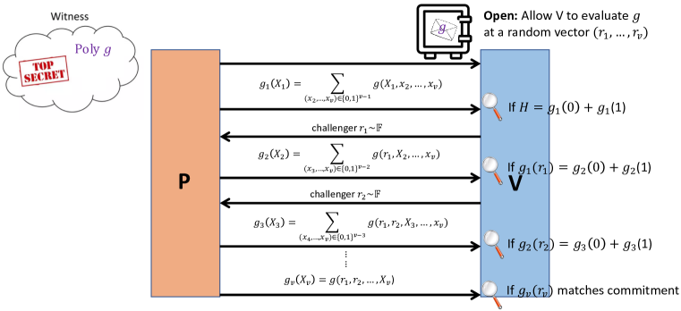
Figure 3: Sum-Check protocol for $H\overset{\text{?}}{=}\sum_{(x_{1},x_{2},...x_{v})\in\{0,1\}^{v}}g(x_{1},x_{2},...,x_{v})$.

Algorithm 2 Sum-Check protocol (interactive) for Equation (11)

1:Commitment: Prover commits to the polynomial $g$ and sends the Pedersen commitment of $g$ to verifier (with an ability to prove the evaluation $g(r_{1},r_{2},...,r_{v})$ at any point $(r_{1},r_{2},...,r_{v})$, see Algorithm 1).

2:Prover computes the polynomial with the argument $X_{1}$: $g_{1}(X_{1})=\sum_{(x_{2},...,x_{v})\in\{0,1\}^{v-1}}g(X_{1},x_{2},...,x_{v})$ and sends the polynomial to verifier.

3:if Verifier finds $H\not=g_{1}(0)+g_{1}(1)$ then

4:     Verifier outputs REJECT and ends the algorithm.

5:end if

6:Verifier samples a random number $r_{1}\in\mathbb{F}$ and sends it to prover.

7:for $i=2,3,...,v$ do

8:     Prover computes the polynomial with the argument $X_{i}$: $g_{i}(X_{i})=\sum_{(x_{i+1},...,x_{v})\in\{0,1\}^{v-i}}g(r_{1},...,r_{i-1},X_{i},x_{i+1},...,x_{v})$ and sends the polynomial $g_{i}(X_{i})$ to the verifier.

9:     if Verifier finds $g_{i-1}(r_{i-1})\not=g_{i}(0)+g_{i}(1)$ then

10:         Verifier outputs REJECT and ends the algorithm.

11:     end if

12:     Verifier samples a random number $r_{i}\in\mathbb{F}$ and sends it to prover.

13:end for

14:if Verifier checks that $g_{v}(r_{v})$ matches the opening of the commitment by a proof system in Algorithm 1 then

15:     Verifier outputs PASS.

16:else

17:     Verifier outputs REJECT.

18:end if

Reducing Linear Layers to Sum-Check Protocol. Linear layers frequently appear in foundation models. Mathematically, linear layers can be written as matrix multiplication. Given $n\times n$ matrices $\mathbf{A}$ and $\mathbf{B}$ and we denote $\mathbf{A}\mathbf{B}$ as $\mathbf{C}$. One can interpret $\mathbf{A},\mathbf{B},\mathbf{C}$ as function $f_{A},f_{B},f_{C}:\{0,1\}^{\log_{2}n}\times\{0,1\}^{\log_{2}n}\rightarrow\mathbb{F}$:

$$f_{A}(i_{1},...,i_{\log_{2}n},j_{1},...,j_{\log_{2}n})=A_{ij},$$ (18)

where sequence $(i_{1},...,i_{\log_{2}n})$ and $(j_{1},...,j_{\log_{2}n})$ are the binary representations of $i$ and $j$, respectively. Let $\widetilde{f_{A}},\widetilde{f_{B}},\widetilde{f_{C}}:\mathbb{F}^{\log_{2}n}\times\mathbb{F}^{\log_{2}n}\rightarrow\mathbb{F}$ denote the multilinear extension of $f_{A},f_{B},f_{C}$. It is easy to check that

$$\widetilde{f_{C}}(i_{1},...,i_{\log_{2}n},j_{1},...,j_{\log_{2}n})=\sum_{\mathbf{b}\in\{0,1\}^{\log_{2}n}}\widetilde{f_{A}}(i_{1},...,i_{\log_{2}n},\mathbf{b})\cdot\widetilde{f_{B}}(\mathbf{b},j_{1},...,j_{\log_{2}n}).$$ (19)

Equation (19) is in the form of (11). Thus, we can apply the Sum-Check protocol for verifying the execution of linear layers with $\log_{2}n$-variant, degree-2 polynomial $g(\mathbf{b})=\widetilde{f_{A}}(i_{1},...,i_{\log_{2}n},\mathbf{b})\cdot\widetilde{f_{B}}(\mathbf{b},j_{1},...,j_{\log_{2}n})$ and $H=\widetilde{f_{C}}(i_{1},...,i_{\log_{2}n},j_{1},...,j_{\log_{2}n})$ at a random point $(i_{1},...,i_{\log_{2}n},j_{1},...,j_{\log_{2}n})\in\mathbb{F}^{\log_{2}n\times\log_{2}n}$.

2.1.8 Proofs for Non-Arithmetic Operations

There are two major techniques for zero-knowledge proof of non-arithmetic operations: 1) bit decomposition and 2) lookup table.

Reducing ReLU Activation to Bit Decomposition. Bit decomposition is one of the most frequently used techniques for zero-knowledge proofs of non-arithmetic operations. Let $\mathbf{Z}$ denote the pre-activated tensor of ReLU, and let $\mathbf{A}$ denote the after-activated tensor. We now introduce the techniques appearing in [11]. In the ReLU activation, we have

$$\mathbf{A}=\text{sign}(\mathbf{Z})\odot\text{abs}(\mathbf{Z}),$$ (20)

where $\odot$ is the Hadamard product, $\text{abs}(z)$ is the element-wise absolute value of $\mathbf{Z}$, and

$$\text{sign}(z)=\begin{cases}0,&\text{if $z<0$};\\ 1,&\text{otherwise},\\ \end{cases}$$ (21)

is applied element-wise to the tensor $\mathbf{Z}$. Denote by $z=(z_{0},z_{1},...,z_{Q})$ the Q-bit binary representation of $z$, where $Q=\log_{2}p$ (e.g., 128 or 256), $p$ is the (prime) order of the finite field $\mathbb{F}$, $z_{0}=\text{sign}(z)\in\{0,1\}$ represents the sign, and $(z_{1},...,z_{Q})=\text{abs}(z)$ refers to the Q-bit unsigned binary representation of $z$. To prove Equation (20) holds for all elements $z$, we only need to prove: 1) $(z_{0},z_{1},...,z_{Q})$ is binary representation such that all elements are in $\{0,1\}$: $0\overset{\text{?}}{=}z_{i}(z_{i}-1)$ for $i\in\{0,1,...,Q\}$; 2) $(z_{0},z_{1},...,z_{Q})$ can recover $z$ in the sense that

$$z\overset{\text{?}}{=}\underbrace{(2\times z_{0}-1)}_{\text{sign}}\times\underbrace{(2^{Q-1}\times z_{1}+2^{Q-2}\times z_{2}+...+2^{0}\times z_{Q})}_{\text{Q-bit unsigned integer}};$$ (22)

and 3) Equation (20) is correctly executed for element $a\in\mathbf{A}$ in the sense that

$$a\overset{\text{?}}{=}z_{0}\times(2^{Q-1}\times z_{1}+2^{Q-2}\times z_{2}+...+2^{0}\times z_{Q}).$$ (23)

Therefore, with bit decomposition, we can reduce the non-arithmetic ReLU operation to the arithmetic operations in the proofs of 1) and 2) and call the Sum-Check protocol. We can also use the Schwartz-Zippel Lemma to merge all the proofs in 1) and 2) into a single one:

$$\begin{split}&(2z_{0}-1)(2^{Q-1}z_{1}+...+2^{0}z_{Q})-z+(z_{0}(2^{Q-1}z_{1}+...+2^{0}z_{Q})-a)r\\ &+\sum_{i=0}^{Q}z_{i}(z_{i}-1)r^{i+2}\overset{\text{?}}{=}0,\end{split}$$ (24)

where $r\sim\mathbb{F}$ is a random sample from the finite field $\mathbb{F}$.

Reducing Non-Arithmetic Operations to Lookup Tables. A lookup table is another technique for zero-knowledge proofs of non-arithmetic operations. It resolves the issue in the bit decomposition approach that the binary representation is lengthy when $p$ is large, so one non-arithmetic operation is represented by as many as $\log_{2}p$ bit-operations [18]. Hereby, the length of $\log_{2}p$ comes from the use of base-2 in the bit decomposition. In order to resolve the issue, one could consider a larger base $k$ and check the correction of base-$k$ decomposition by a table lookup. We now introduce the techniques appearing in [13]. In particular, both the prover and the verifier parties maintain a shared table: $\mathcal{T}:=\{(\mathbf{T}_{\mathcal{X}},f(\mathbf{T}_{\mathcal{X}}))\}\in\mathbb{F}^{n_{2}\times(d_{1}+d_{2})}$ for a non-arithmetic operation $f$ (e.g., the Softmax operation). To reduce the non-arithmetic operation $f$ to a lookup table argument, the prover needs to convince the verifier that the $d_{1}$-dim input vector $\mathbf{X}$ and the $d_{2}$-dim output vector $\mathbf{Y}$ satisfy $\sum_{i=0}^{d_{1}-1}r^{i}\mathbf{X}_{i}+\sum_{i=0}^{d_{2}-1}r^{i+d_{1}}\mathbf{Y}_{i}\subset\sum_{i}\textsf{Col}_{i}(\mathcal{T})r^{i}$ for a random $r\sim\mathbb{F}$, where $\textsf{Col}_{i}(\mathcal{T})$ refers to the $i$-th column of table $\mathcal{T}$. One can further reduce the proof of this “subset” relations to a Sum-Check proof, by observing that: $\mathbf{S}\subset\mathbf{T}$ for $\mathbf{S}\in\mathbb{F}^{n_{1}}$ and $\mathbf{T}\in\mathbb{F}^{n_{2}}$, if and only if there exists $\mathbf{e}=(e_{0},e_{1},...,e_{n_{2}-1})\in\mathbb{F}^{n_{2}}$ such that the following two polynomials over $X$ is identical:

$$\prod_{i\in[n_{1}]}(X+\mathbf{S}_{i})=\prod_{i\in[n_{2}]}(X+\mathbf{T}_{i})^{e_{i}}.$$ (25)

By taking the logarithmic derivative at both sides, the following two rational functions are identical:

$$\sum_{i\in[n_{1}]}\frac{1}{X+\mathbf{S}_{i}}=\sum_{i\in[n_{2}]}\frac{e_{i}}{X+\mathbf{T}_{i}}.$$ (26)

The prover sets and commits to $e_{i}=|\{j:\mathbf{S}_{j}=\mathbf{T}_{i}\}|$. Equation (26) can be proved by the Sum-Check protocol with a random variable $X\sim\mathbb{F}$, as all the operations here are arithmetic [13].

2.1.9 Zero-Knowledge Proofs for Foundation Models

Table 2: Zero-knowledge proof techniques for various operations in foundation models.

Operations	Zero-Knowledge Proof Techniques
Linear Layer [18]	Sum-Check Protocol
Convolution [12]	Sum-Check Protocol/FFT
Residual Connection [13]	Sum-Check Protocol
Softmax/Sigmoid/SwiGLU/GELU/GLU [13]	Lookup Table
LayerNorm/RMSNorm [13]	Lookup Table
ReLU [11]	Bit Decomposition

By integrating all components, one can construct a zero-knowledge proof system for foundation models like Meta’s LLaMA series. Foundation models comprise transformer layers followed by MLP layers. For arithmetic operations, such as the linear layers in transformers and MLPs, the Sum-Check protocol can be effectively employed to generate proofs. For non-arithmetic operations, like Softmax and SwiGLU activation, a lookup table can be utilized. For piece-wise linear activation, such as ReLU, bit decomposition can be used. Table 2 lists the zero-knowledge proof techniques for different operations in foundation models. Note that each operation requires carefully designed techniques for efficiency. To the best of our knowledge, zkLLM [13] is the first work that introduces zero-knowledge proofs to foundation models with tens of billions of parameters such as OPT [21] and LLaMA-2 [22].

2.1.10 zkDPS: Zero-Knowledge Decentralized Proof System at Nesa

At Nesa, we build a zero-knowledge system, zkDPS, for decentralized large language models. zkDPS is built upon zkLLM [13] and zkDL [11]. zkLLM [13] and zkDL [11] are state-of-the-art CUDA implementation of zero-knowledge proofs of machine learning. However, speed remains the most significant pain point for zero-knowledge proofs of foundation models. For example, it takes zkLLM roughly 15 minutes to generate a proof for the inference procedure of LLaMA-2 13B with an input token length of 2,048 [13]. In comparison, vanilla inference of zkLLM takes less than 0.1 seconds per token. Despite significant efforts have been made to accelerate generic zero-knowledge proof frameworks such as zk-STARK and zk-SNARK [23], they are still not fast enough, even much slower than zkLLM for billion-scale models. Therefore, the acceleration of zero-knowledge proofs is urgent for real-world applications.

zkDPS proposes the following ideas to speed up proof generation beyond zkLLM [13] and zkDL [11]. One idea could be to leverage the “compressible property” of LLMs by algorithmic innovation. It is well-known that LLMs are in essence a compression of information and data from the real world. Thus one could consider using a small draft model to “guess” the output of the original LLM, similar to speculative sampling. As the draft model is small (typically 20x-50x smaller than the original LLM [24]), one could expect to experience a shorter time for proof generation of the execution of the draft model. Experimentally, the top-1 guessing accuracy of the draft model is as high as 82% in EAGLE [24, 25], a state-of-the-art speculative sampling method. Therefore, this acceleration technique will not degrade the inference performance of LLMs too much.

Another idea is to leverage the hardware acceleration of modern GPUs. zkLLMs has already used CUDA implementation to parallelize the computations in the proof generation. For example, the CUDA kernels such as Pedersen commitment, elliptic curve, and lookup tables have been re-implemented or adapted in zkLLMs [13, 11], making it the fastest implementation of zero-knowledge large language models at the submission of this paper. In Nesa, we are optimizing those kernels by engineering methods such as Tensor Parallelism and KV cache.

2.2 Sequential Vector Encryption

At Nesa, we have designed an innovative encryption method called Sequential Vector Encryption (SVE) which is a robust scheme inspired by our diagrammatic interpretation of homomorphic encryption applied on select linear layers rather than the full model. In particular, we focus on the modern LLM architecture but this framework can be applied to other types of neural networks such as CNNs. We consider the LLM to be a sequence of vector space operators. As mentioned previously, this sequence contains both linear and non-linear operators. In principle, the (intermediate) output vector of every operator contains information about both the input and the output of the model. We sometimes refer to this operator output as a (latent) representation vector, as it is a representation of the input data after (partial) processing through some intermediate computational operations in the neural network. We wish to apply SVE when there is some extra concern that an attacker can access these vectors and, subsequently, can extract sensitive information attributed to either the initial model input or model output. Our method focuses on obfuscating the output of every operator in the sequence of the LLMs so that any observation of the neural representation of the data in any intermediate latent space is not usable for this purpose. This extra level of security is particularly relevant for the use of models that heavily rely on open-source foundation models for which the intermediate latent spaces are available for extensive study by any actor.

The general technique for SVE is based on the simple idea of randomly transforming the outputs of every operator so that the intermediate vector representations can no longer be interpretable using a given method developed for the original model’s vector representations. In order to be usable for the original model, these representations need to be transformed into the original representation space before feeding to the next operator. Equivalently, we can transform the operator itself to the operator on the transformed vector space in the correct way, instead of transforming the vector itself, which is how the technique is implemented in practice as this allows efficient secret sharing - to be discussed below. In either case, the computational complexity of the transformation is the same. As the intermediate representations have dimensionalities on the order of roughly $10^{3}$ components (for reference a small LM such as BERT typically uses 768 dimensions and Llama 2 uses 4096 dimensions), any attempt to recover the transformed vectors means determining the parameters of the transformation (representable as a matrix), which are on the order of $10^{6}$ floating point parameters for a typical transformation. This would amount to solving a very large undetermined system.

There are two main considerations to put this into practice: (1) an appropriate transformation of each operator, and (2) a secret sharing method so that transformation matrices are never revealed during operation. The former (1) ensures that the transformations preserve the computational outputs of the original model and the latter (2) is required so that no agent can recover the encrypted representation vectors. The following will explain how we address both considerations.

Appropriately transforming each operator depends on the type of operator under consideration, for a linear operation, it can be transformed as a product of (invertible) transformation matrices and the original matrix representation of that operator (recoverable from the original LLM). For non-linear operators, we can take advantage of certain symmetries of the operator. For instance, the ReLU $R$ operator is pointwise, and thus $R$ commutes with any vector space permutation $P$ according to the following diagram:

Here we are transforming between real vector spaces of the same dimension. Since $P$ is always invertible, this diagram tells us that we can represent the ReLU operator as $R^{\prime}=P^{-1}RP$. This transformation alone is not necessarily enough to obscure the transformation as a bad actor with knowledge of the layer could in principle run a known vector through the open source model and compare the two representation vectors component-wise to figure out the transformation. Therefore we can scale with a random vector with all positive entries, as the $R$ also fits into the following commutative diagram:

where $M_{a}$ is multiplication by $a\in\mathbb{R}^{n}_{>0}$, a diagonal matrix with positive diagonal terms. Concatenating the two transformations we obtain the representation $R^{\prime\prime}=M_{a}^{-1}R^{\prime}M_{a}=M_{a}^{-1}P^{-1}RPM_{a}$, noting that any diagonal matrix with non-zero diagonal entries is invertible. As an aside, it is interesting to note that the number of per- mutations on an n-dimensional vector are simply n!, so even for BERT, the number of possible permutations is 768! whereas it is thought that there are roughly 60! atoms in the universe. Other nonlinear operators can be transformed using similar, but more careful, considerations. We finally package our transformation $T=PM_{A}$ as a single matrix $T$, with corresponding inverse $T=M_{a}^{-1}P^{-1}$. However, revealing this matrix directly in the procedural code distributed to agents will compromise security. Thus we use a form of secret sharing to obfuscate the transformation matrices.

To see how secret sharing can be incorporated in SVE, it is illuminating to consider how to transform a linear/nonlinear pair of operators as this is the basic structure of most neural network layers, including LLMs. We represent the single (original) $i$th layer $B_{i}$ as

$${B_{i}=RA},$$ (27)

where $A$ is a linear transformation and $R$ is our nonlinear ReLU as above. Consider $\overline{A}=SA$, where $S$ is the appropriate transformation matrix, and $\overline{R}=T^{-1}RT$, where $T$ is defined above. Then

$$\begin{split}\overline{B_{i}}&=\overline{R}\overline{A}\\ &=(T^{-1}RT)(SA)\\ &=T^{-1}(RTSA)\\ &=T^{-1}RC,\end{split}$$ (28)

where $C=TSA$ is a new matrix transformed from the original matrix $A$. Here we assume the output of the previous block is transformed according to $S^{1}$, and the output of $\overline{B_{i}}$ will be equivalent to the output of $B_{i}$ transformed by $T^{-1}$. Now the transformation pair $S$ and $S^{-1}$ cannot be recovered by the above agent but the transformation $T^{-1}$ is recoverable, which allows $S$ to also be recoverable with (public) knowledge of $A$. Thus by looking ahead to the next layer $B_{i+1}$ we can insert the appropriate transformation pair $U$ and $U^{-1}$ by absorbing $U^{-1}$ in to the linear representation for $B_{i+1}$ and using the representation

$$\overline{B_{i}}=UT^{-1}RC=GRC,$$ (29)

where $G=UT^{-1}$. Now the layer $B_{i}$ as $GRC$ appropriately transforms the layer so that none of the matrices $T^{-1}$, $U$, $T$ or $S$ can be recovered.

A final attack can be made if two agents in sequence collude. We mitigate this by injecting additional transformations in the sequential chain of operators, similar to how the transformation $G$ was constructed. These additional operators are sent, along with the encrypted representation vector at this point in the sequence to run on either a trusted third party such as a TEE, or on the original client to sequentially encrypt the representation vector. Thus, the encrypted outputs are always passed back to the holder of this additional transformation. This topology is natural in the sense of a decentralized network this can be performed at the same time as consensus is verified.

3 Security and Privacy for General Inference

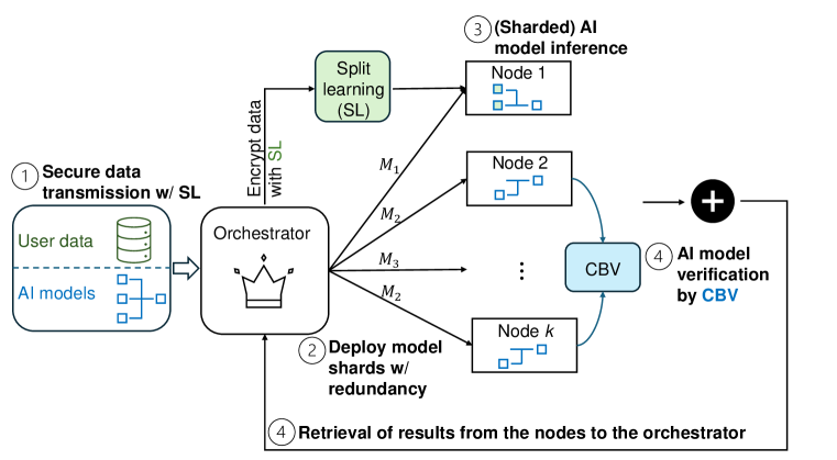
Figure 4: Security flowchart for general inference, where Nesa designs CBV (§3.1) for model verification and leverages SL (§3.2) for data encryption and user privacy protection.

In general inference scenarios, the results of AI inference tasks are less critical, allowing for faster processing speeds and lower costs without compromising basic security and privacy standards. These tasks include everyday activities such as checking the weather, recommending products, or filtering spam emails. Our strategy for ensuring model verification and integrity in these scenarios is Consensus-based Verification Check (CBV), which leverages the collective agreement of multiple nodes to ensure the correctness and integrity of model execution without revealing sensitive data. This approach is detailed in Section 3.1. For data privacy, we employ split learning (SL) [14, 26], a method where the model is divided into segments, and each segment is trained on different nodes to maintain data privacy by ensuring no single node has access to the complete dataset. More information on this technique can be found in Section 3.2. Fig. 4 provides an overview of the security flow of general inference at Nesa which first applies SL to encrypt the first (few) layers to “encrypt” the raw data, where the AI models are sharded and deployed to nodes with redundancy. For the nodes who have the same shard, their outputs will be verified by consensus for integrity.

3.1 Consensus-based Verification Check for Model Integrity

Given the computational and scalability challenges associated with ZKML for verifying the integrity of LLMs in decentralized systems, Nesa proposes a consensus-based distribution verification (CDV) strategy for general inference scenarios. This strategy leverages the collective agreement of multiple nodes to ensure the correctness and integrity of model execution without revealing sensitive data.

Consensus-based Verification. Consider a decentralized network with $N$ nodes, where each node $i$ executes the same inference model $\mathcal{M}$ with parameters $\theta$, on a given input $x$ [27]. The output of the model on node $i$ is denoted by $y_{i}=\mathcal{M}(x;\theta_{i})$. The goal is to ensure that all nodes accurately execute the model $\mathcal{M}$, yielding consistent outputs. The process can be formalized in the following steps:

1. Redundant execution. A subset of the network nodes, $\{1,2,\ldots,k\}\subseteq N$, independently computes the output $y_{i}$ for the same input $x$.

   $$y_{i}=\mathcal{M}(x;\theta),\quad\forall i\in\{1,2,\ldots,k\}.$$ (30)

2. Output collection. The outputs $\{y_{1},y_{2},\ldots,y_{k}\}$ are collected for consensus evaluation. This collection phase requires secure and efficient communication protocols to protect the integrity of the transmitted data.

3. Consensus determination. Utilizing a consensus algorithm $\mathcal{C}$, the system evaluates the collected outputs to determine the agreed-upon result $y_{\text{con}}$. The consensus result is considered valid if it satisfies a predefined criterion, such as majority agreement or a more sophisticated decision rule based on the specific properties of the outputs.

   $$y_{\text{con}}=\mathcal{C}(\{y_{1},y_{2},\ldots,y_{k}\}).$$ (31)

4. Verification and finalization. If the consensus results $y_{\text{con}}$ align with the outputs from a sufficiently large subset of nodes, the model’s execution is verified. Otherwise, discrepancies indicate potential integrity issues, triggering further investigation or corrective measures.

This consensus-based approach not only facilitates the verification of model integrity across decentralized nodes but also introduces a robust mechanism to detect and mitigate the impact of faulty or malicious nodes.

Taking Model Sharding into Account. In Nesa’s decentralized system, where ML models’ computational graphs may be sharded across multiple nodes for scalability, each node $i$ possesses a unique shard $\mathcal{M}_{i}$ of the complete model $\mathcal{M}$. This partitioning requires a specialized approach to Consensus-based Verification to accommodate the fragmented nature of model execution.

Consider the complete model $\mathcal{M}$ being divided into $k$ shards, such that $\mathcal{M}=\bigoplus_{i=1}^{k}\mathcal{M}_{i}$, where $\bigoplus$ denotes the operation of combining the model shards to represent the full model functionality. Given an input $x$, the execution of these shards across $k$ nodes produces a set of partial outputs $\{y_{1},y_{2},\ldots,y_{k}\}$, where $y_{i}=\mathcal{M}_{i}(x;\theta_{i})$.

Verification in the Context of Sharding.

1. Shard Redundant Execution. For each shard $\mathcal{M}_{i}$ of the complete model $\mathcal{M}$, redundant execution is performed by a designated subset of nodes. Each of these nodes, within the subset responsible for shard $\mathcal{M}_{i}$, computes the output $y_{i,j}$ for the given input $x$, where $j$ represents the node within the subset.

   $$y_{i,j}=\mathcal{M}_{i}(x;\theta_{i,j}),\quad\forall j\in\text{Subset of nodes for }\mathcal{M}_{i}.$$ (32)

   This step introduces computational redundancy, where multiple independent computations of the same shard aim to fortify the verification process by cross-verifying results among nodes computing the same shard.

2. Redundant Output Collection and Verification. The outputs $\{y_{i,1},y_{i,2},\ldots,y_{i,m}\}$ for each shard $i$ are collected from the nodes in its subset. A consensus mechanism $\mathcal{C}_{i}$ specific to shard $i$ then evaluates these collected outputs to determine a shard-specific agreed-upon result $y_{\text{con},i}$.

   $$y_{\text{con},i}=\mathcal{C}_{i}(\{y_{i,1},y_{i,2},\ldots,y_{i,m}\}).$$ (33)

   Here, $m$ denotes the number of nodes executing the shard $\mathcal{M}_{i}$. The redundancy in computation across these nodes allows for a robust verification mechanism, enhancing the detection of discrepancies or faults.

3. Shard Verification Completion. Upon achieving consensus for a shard $i$, signified by the result $y_{\text{con},i}$, the process ensures the integrity of the shard’s computation before proceeding. This step-by-step verification across shards, with redundancy in each shard’s computation, significantly reduces the risk of erroneous or malicious model execution.

4. Model Reconstruction. After each shard has been independently verified, the shard-specific consensus results $\{y_{\text{con},1},y_{\text{con},2},\ldots,y_{\text{con},k}\}$ are combined to reconstruct the final model output $Y_{\text{final}}$. This comprehensive output can ensure the integrity of the complete model execution.

   $$Y_{\text{final}}=\bigoplus_{i=1}^{k}y_{\text{con},i}.$$ (34)

Consensus-based Distribution Verification (CDV). Building upon traditional consensus mechanisms, the CDV strategy introduces an advanced layer of verification by assessing the statistical distribution of model outputs across a decentralized network. This approach is ideally suited for scenarios where the model is not monolithic but is instead distributed as shards across multiple nodes.

CDV is based on the understanding that while individual outputs from model shards might exhibit slight variability due to the stochastic nature of ML models and the complexity of input data, the collective output distribution should maintain consistency. This consistency holds, provided that the model and its inputs remain unchanged. By evaluating the aggregated statistical characteristics of these outputs, CDV furnishes a sophisticated and robust framework for affirming the uniformity and integrity of the model’s behavior, thereby enhancing security and privacy without direct comparison of individual inference results.

• Sharded Execution and Output Synthesis. In the initial phase, each node, housing a shard $\mathcal{M}_{i}$ of the overarching model $\mathcal{M}$, executes its segment on a shared input $x$, generating partial outputs $\{y_{1},y_{2},\ldots,y_{k}\}$. These outputs are synthesized to construct a comprehensive output profile reflecting the entire model’s combined inference result.

• Advanced Statistical Aggregation. Following output synthesis, the system embarks on advanced statistical analysis, deriving metrics such as the mean $\mu$, standard deviation $\sigma$, and potentially higher-order moments. This stage may also incorporate non-parametric statistics to capture the full essence of the output distribution, offering a nuanced view of the model’s performance landscape.

• Rigorous Distribution Comparison. Utilizing sophisticated statistical methodologies, the derived metrics are juxtaposed with predefined benchmarks or dynamically established norms. Techniques such as hypothesis testing, divergence measures, or similarity indices evaluate the congruence between the observed and expected output distributions, facilitating an objective assessment of model integrity.

• Enhanced Consensus Mechanism with Adaptive Thresholding. The core of CDV lies in its consensus mechanism, where nodes collectively determine the acceptability of the observed distribution’s alignment with benchmarks. Adaptive thresholding plays a crucial role here, dynamically adjusting sensitivity based on historical data and operational context to pinpoint deviations that truly signify integrity breaches.

Through its implementation, CDV offers a powerful solution to the challenges of verifying the integrity of distributed ML models in Nesa’s decentralized framework. By focusing on distributional characteristics rather than discrete output values, CDV not only elevates the verification process but also aligns with the goals of enhancing model security and maintaining stringent privacy standards.

3.2 Data Privacy Protection via Split Learning

Recognizing the challenges posed by encrypting data for use in decentralized inference systems, Nesa adopts Split Learning (SL) as a pragmatic solution to facilitate secure and efficient computation on encrypted data [28, 29]. Traditional encryption methods such as HE, while securing data at rest and in transit, render it costly for direct computation by obscuring its format and structure. This limitation is particularly problematic for processing with LLMs within a decentralized framework, where data privacy cannot be compromised.

Split Learning [14] addresses these concerns by partitioning the computational model, allowing for data to be processed in parts without revealing sensitive information. In essence, the user data is protected by not being directly transmitted to any nodes – only the data embeddings are being passed around, and each node will only be accessing the embeddings of certain layers.

Consider a neural network model $\mathcal{N}$, such as Llama 2 [30] composed of a sequence of 32 layers $\{L_{1},L_{2},\ldots,L_{32}\}$, each with its own set of parameters $\Theta_{i}$ and activation function $\sigma_{i}$. The input to the network is $X$, and the output of the $i$-th layer, given input $x_{i}$, can be mathematically described as:

$$a_{i}=L_{i}(x_{i};\Theta_{i})=\sigma_{i}(W_{i}x_{i}+b_{i}),$$ (35)

where $W_{i}$ and $b_{i}$ are the weight matrix and bias vector of the $i$-th layer, respectively, and $\sigma_{i}$ is a nonlinear activation function such as ReLU, sigmoid, or tanh.

Assuming the model is split at layer $k$, where the client handles layers $\{L_{1},\ldots,L_{k}\}$ and the server handles layers $\{L_{k+1},\ldots,L_{32}\}$. The client computes the intermediate representation $Z$ as follows:

$$Z=\sigma_{k}(W_{k}\cdot\sigma_{k-1}(\ldots\sigma_{1}(W_{1}X+b_{1})\ldots)+b_{k}).$$ (36)

This intermediate representation $Z$ is then transmitted to the server, which continues the computation:

$$Y=\sigma_{32}(W_{32}\cdot\sigma_{31}(\ldots\sigma_{k+1}(W_{k+1}Z+b_{k+1})\ldots)+b_{32}).$$ (37)

The loss function $\mathcal{L}(Y,Y_{true})$ computes the error between the network output $Y$ and the true labels $Y_{true}$, and the gradient of the loss with respect to the model’s parameters through backpropagation:

$$\frac{\partial\mathcal{L}}{\partial\Theta_{i}}=\text{ChainRule}\left(\frac{\partial\mathcal{L}}{\partial Y},\frac{\partial Y}{\partial a_{32}},\ldots,\frac{\partial a_{i}}{\partial\Theta_{i}}\right).$$ (38)

For privacy concerns during the transmission of $Z$ from client to server, differential privacy methods may be applied [31]. Defining a privacy metric $\mathcal{P}$ that quantifies the information leakage from the intermediate representation $Z$, a proof of privacy preservation could demonstrate that for any $\epsilon$-differential privacy guarantee, the information leakage remains below a threshold:

$$\mathcal{P}(Z)\leq\epsilon.$$ (39)

It is noted that by using differential privacy with SL, the privacy will be improved at the cost of inference quality [32]. Thus, in Nesa’s framework, this is defined as a tunable parameter to be decided, given the user requirements.

By leveraging Split Learning, Nesa effectively navigates the complexities of data encryption within its decentralized inference system for LLMs. This approach not only preserves the confidentiality and integrity of user data but also ensures the operational feasibility of complex model computations, demonstrating a sophisticated balance between privacy preservation and computational pragmatism.

4 NTEE: Nesa’s Trusted Execution Environments for Security and Privacy

Trusted Execution Environments (TEEs) effectively establish security and privacy within Nesa’s decentralized inference architecture. Using TEEs, we can create secure isolation zones within the network’s nodes, guaranteeing the privacy and accuracy of data and computational operations. In Nesa’s scenarios, two key pieces of information should be protected from the node runners: (i) users’ input data for AI inference and (ii) private model parameters, where TEE provides a hardware-based solution for it.

To ensure the protection of sensitive processes and data within nodes from unauthorized access, including the node operators themselves, TEEs provide an aggressive isolation mechanism. The significance of isolation is of utmost importance in a decentralized setting where the inference of AI models is spread among multiple owners.

1. Isolated Execution. TEEs provide a secure enclave for executing computations, isolated from the rest of the node’s operating environment. This isolation ensures that even if other parts of the node are compromised, the computations within the TEE remain protected. When nodes process only fragments of a model, ensuring the integrity and confidentiality of each fragment is crucial. TEEs prevent any unauthorized access or tampering with the code and data inside the enclave, thus safeguarding the partial model computations.

2. Data Privacy. Since each node handles only parts of the AI model, sensitive data processed by the model can potentially be less secure if exposed to less protected parts of the system or network. TEEs encrypt the data within the enclave, ensuring that any information processed remains confidential. Even if data needs to be shared across nodes, it can be encrypted before leaving the TEE, ensuring that it travels securely across the network.

3. Consistency and Integrity. TEEs can ensure the integrity of the computations performed on each node. Through cryptographic techniques such as attestation, a TEE can prove to other nodes or external verifiers that the computations were performed correctly without revealing the underlying data. This attestation process allows other nodes in the decentralized network to trust the results from each node without having to access the actual data or model details, thus maintaining consistency and integrity across the decentralized model.

CPU- and GPU-based TEEs. Intel, AMD, and NVIDIA all provide TEEs, while NVIDIA uniquely supports GPU TEEs. This capability is crucial for accelerating AI and high-performance computing tasks securely, where GPUs can efficiently handle tensor-based operations. The general procedure involves initializing a CPU TEE virtual machine (VM) first, which then controls the GPU TEE (available only with NVIDIA). This setup ensures that the owner of the CPU and GPU cannot see the contents of the VM, providing an additional layer of security. In other words, even though the node runner owns the hardware, they cannot access the AI model and data inside the VM.

By leveraging TEEs, Nesa can provide robust security and privacy measures that are essential for both critical and general inference scenarios, ensuring that sensitive data and model parameters are always protected from unauthorized access and tampering. Thus, we design a specialized version of TEEs, named NTEE, that best suits Nesa’s scenarios with decentralized inference. Note that NTEE is feasible for all node runners with or without GPUs.

The Advantages of TEEs include:

• Low Overhead and High Performance: TEEs provide a secure computing environment with minimal performance overhead (i.e., can be as small as 3% as reported in different literature [33, 34]), ensuring efficient execution of AI inference tasks. This allows Nesa to maintain high performance in both critical and general inference scenarios.

• Support for Both CPU and GPU: TEEs can be implemented on both CPUs and GPUs, with the general procedure involving initializing a CPU TEE virtual machine (VM) that controls the GPU TEE (available only with NVIDIA). This setup, supported by NVIDIA H100 Tensor Core GPUs, ensures seamless interaction with the hardware and enhances the security of AI computations.

• Data and Model Security: The hardware owner (node runner) will not have access to the AI model and data inside the VM. This ensures the confidentiality and integrity of the computations, protecting sensitive data and model parameters from unauthorized access, even by the hardware owners.

• Elimination of Algorithm-Based Approaches: Utilizing TEEs negates the need for algorithm-based security measures like ZKML and HE discussed above in §2.1 and 2.2. This results in faster performance due to the inherent efficiency of hardware-based security, making it ideal for Nesa’s decentralized AI inference tasks.

• Scalable and Secure Collaboration: TEEs enable secure collaboration across multiple nodes by creating isolated enclaves that protect data during computation. This is particularly beneficial for Nesa’s decentralized AI inference, allowing multiple organizations to pool their data securely for training and inference while maintaining data privacy and compliance.

4.1 Implementation of NTEE in Details

Nesa, as a decentralized AI provider, aims to have multiple node runners collaboratively leverage their hardware to perform AI inference for users. In this setup, Nesa employs one orchestrator within the Rich Execution Environment (REE) to facilitate the entire process within NTEE. The REE, unlike the TEE, is the standard, general-purpose operating environment that handles regular applications and processes without the enhanced security measures of a TEE. We have the user data $\mathbf{X}$ and the AI model $M$ (e.g., Llama 2 [30]), and we have $k$ node runners for hosting TEEs. Fig. 5 provides a high-level overview of our implementations of NTEE.

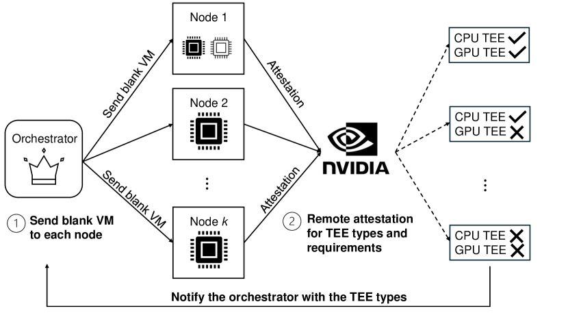
(a) The first two steps are (1) sending an empty secure VM (without any data and models) to each node runner by the orchestrator and (2) running remote attestation with the server provider like NVIDIA to ensure the types of TEEs a node can support.

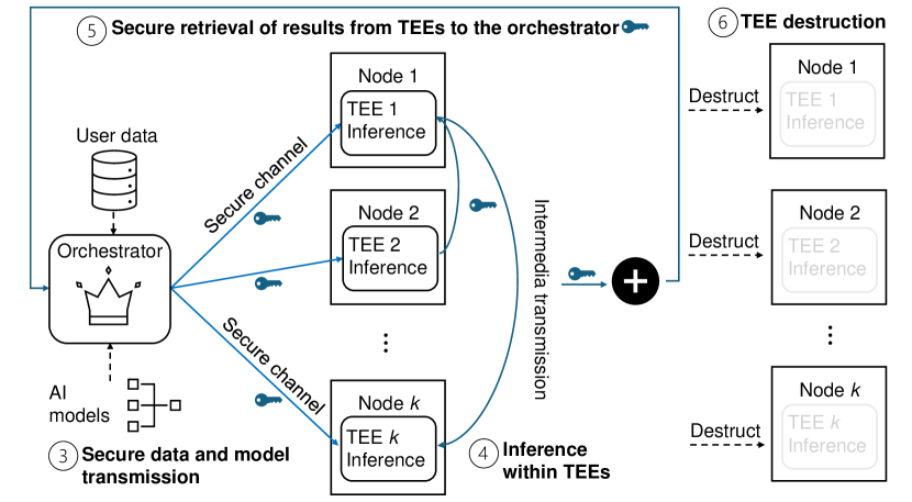
(b) After knowing the TEE types each node can support, the orchestrator (3) sends user data and AI models to each node’s TEEs via the secure channel, after which (4) nodes execute AI inferences within TEEs and directly communicate with each other via secure channels. Finally, The orchestrator (5) retrieves the aggregated results from TEEs securely and notifies the node runners to destroy each TEE.

Figure 5: Overview of Nesa’s NTEE paradigm for decentralized AI inference.

Step 1: TEE Initialization. Nesa first sends a blank Virtual Machine (VM) TEE to each node runner. This VM does not contain any data or model information initially, ensuring no sensitive information is at risk during the setup phase.

Step 2: Remote Attestation. The orchestrator initiates ”remote attestation” with NVIDIA to verify that the node runner’s machine meets the requirements for NVIDIA’s TEE. Remote attestation involves the following steps:

1. The attester (TEE) collects a set of claims that represent the state of its system, including a cryptographic hash of the application’s code:

   $$\text{Measurement}=H(\text{Code}),$$

   where $H$ denotes a cryptographic hash function.

2. These claims, along with the hardware state, are signed to form evidence:

   $$\text{Evidence}=\text{Sign}_{\text{Private Key}}(\text{Claims}).$$

3. The evidence is sent to the verifier, who checks its validity using the public key:

   $$\text{Verify}(\text{Evidence},\text{Public Key})\rightarrow\text{True/False}.$$

4. Based on the attestation results, the orchestrator determines whether each node supports GPU TEE or CPU TEE only:

   $$\text{TEE Type}=\begin{cases}\text{GPU TEE},&\text{if GPU TEE requirements met};\\ \text{CPU TEE},&\text{if only CPU TEE requirements met}.\end{cases}$$

   If the machine meets the requirements for a GPU TEE, the NVIDIA toolkit is used to initialize the GPU VM. Otherwise, only a CPU-based VM is initialized.

If the machine meets the requirements for a GPU TEE, the NVIDIA toolkit can be used to initialize the GPU VM. Otherwise, only a CPU-based VM is initialized. The supported types of TEE information are sent back to the orchestrator.

Step 3: Secure Data and Model Transmission. Once attestation confirms the TEE’s security, Nesa securely transmits the user data $\mathbf{X}$ and the AI model fragment $M_{i}$ to the node runner’s TEE via an encrypted channel, similar to SSH:

$$\text{Secure Transmission:}\quad\text{Enc}(\{\mathbf{X},M_{i}\})\xrightarrow{\text{SSH}}\text{TEE}.$$

Here, Enc denotes encryption, ensuring that the data and model remain confidential and are not exposed to unauthorized access during transit.

Step 4: AI Inference within TEEs. Each node runner’s TEE performs a part of the AI inference using the model fragment $M_{i}$ on the data $\mathbf{X}$. The TEE provides an isolated environment for secure computation, ensuring the node runner cannot access the sensitive data or model parameters. The computation within the TEE can be denoted as:

$$\text{Inference:}\quad Y_{i}=M_{i}(\mathbf{X}).$$

For sequential tasks, the orchestrator sets up encrypted channels among the nodes with computation dependencies. Each node can directly send and receive intermediate inference results to and from other dependent nodes (the details are provided in the next section):

$$\text{Intermediate Transmission:}\quad\text{Enc}(Y_{i})\xrightarrow{\text{Encrypted Channel}}\text{Next Node}$$

Step 5: Secure Retrieval of Final Results. After the final computation is completed, the final inference results $Y_{k}$ are securely transmitted back to the orchestrator from the last node’s TEE using an encrypted channel like SSH:

$$\text{Secure Retrieval:}\quad\text{Enc}(Y_{k})\xrightarrow{\text{SSH}}\text{Orchestrator}$$

Step 6: Destruction of TEE. Once the inference results have been successfully retrieved and verified, the TEE on the node runner is destroyed. This step ensures that any residual data or model information is completely removed from the node runner’s hardware. The process can be formalized as:

Destroy TEE:

$$\text{Step 1: Securely erase all data and model information};$$

$$\text{Step 2: Shut down the TEE}.$$

By implementing TEEs in this manner, Nesa ensures that the AI inference process is secure, protecting both the user’s data and the AI model throughout the entire lifecycle of the computation. This approach leverages the robustness of hardware-based security measures, providing high performance and strong guarantees of confidentiality and integrity. TEEs also facilitate mutual attestation, where both the user and the node runner can verify each other’s integrity, further enhancing the trustworthiness of the decentralized AI system.

4.2 Nesa’s Innovation of NTEE

Nesa operates in a unique decentralized AI setting, distinct from the general usage of TEEs where only one REE interacts with one TEE to run a model or a specific task. Nesa’s system involves multiple TEEs across various nodes to run a shard of an AI model, requiring advanced strategies to ensure efficiency and security.

Innovation 1: Communication Optimization Among Multiple TEEs. Nesa optimizes communication by minimizing data transfer between the orchestrator (considered as a REE) and each TEE. Instead of routing all communications through the orchestrator, we establish pre-set secure communication channels among the TEEs. This allows TEEs to communicate directly with each other, significantly reducing latency and improving overall system efficiency. Direct communication between TEEs is secured using encrypted channels to ensure data privacy and integrity during transit, and the owners of the nodes cannot see the communication either. This approach reduces bottlenecks and enhances the speed of decentralized inference processes, which is crucial for real-time applications.

$$\text{Direct Communication:}\quad\text{TEE}_{i}\xrightarrow{\text{Encrypted Channel}}\text{TEE}_{j}$$

Let us assume we have $k$ node runners (each with a TEE), but only $l$ of them need secure communication ($l<k$) due to the sharding, The process involves establishing secure communication channels among the required TEEs through a series of steps to ensure encrypted data transmission and mutual trust. This approach optimizes communication and enhances security without unnecessary complexity.

Note that these TEEs are both attested and verified, so they can establish secure communication channels using a key exchange protocol. This can be done using the Diffie-Hellman key exchange [35], where each pair of TEEs generates a shared secret key:

$$\text{Shared Secret Key}_{ij}=g^{a_{i}b_{j}}\mod p.$$

From this shared secret key, a session key is derived using a key derivation function (KDF):

$$\text{Session Key}_{ij}=\text{KDF}(\text{Shared Secret Key}_{ij}).$$

The session key is used to encrypt the data transmitted between the TEEs, ensuring confidentiality and integrity:

$$\text{Encrypted Data}_{ij}=\text{AES}_{\text{Session Key}_{ij}}(\text{Data}).$$

By following these steps, Nesa ensures that the TEEs needing secure communication can transmit data securely and efficiently. This method reduces the reliance on the orchestrator for data routing, minimizes latency, and leverages the computational strengths of both GPU TEEs and CPU TEEs. The secure communication channels maintain data privacy and integrity throughout the decentralized AI inference process.

Innovation 2: Heterogeneous TEE Scheduling. In Nesa’s system, TEEs are heterogeneous, meaning they vary in type and computational power, with some nodes supporting GPU TEEs and others only CPU TEEs. To manage this diversity, Nesa employs a dynamic scheduling strategy based on initial attestation results. This attestation determines whether a node supports GPU TEE or CPU TEE only. The motivation behind this is to leverage the strengths of each type of TEE, ensuring that computationally intensive tasks are handled by more capable nodes, thereby optimizing overall system performance.

$$\text{TEE Type}=\begin{cases}\text{GPU TEE},&\text{if GPU TEE requirements met};\\ \text{CPU TEE},&\text{if only CPU TEE requirements met}.\end{cases}$$

The dynamic scheduling strategy involves several innovative steps:

1. Initial Attestation: This step determines the capabilities of each node, identifying GPU TEE or CPU TEE support. By understanding the hardware capabilities, we can tailor the workload distribution to maximize efficiency and performance.

2. Resource Allocation: Based on the attestation outcomes, different shards of the AI model $M$ are assigned to different TEEs according to their computational capabilities. More computationally intensive tasks are allocated to nodes with GPU TEEs, while less demanding tasks are assigned to CPU TEEs. This approach ensures that each node operates within its optimal performance range, enhancing the overall efficiency of the decentralized system.

3. Execution and Communication: Establishing encrypted channels for direct communication between TEEs with computational dependencies reduces the orchestrator’s load and improves efficiency. This direct TEE-to-TEE communication is critical for maintaining low latency and high throughput in distributed AI inference tasks.

Innovative Motivations. The innovations in Nesa’s use of TEEs are driven by several key motivations:

• Security and Privacy: Ensuring the confidentiality and integrity of user data and AI models is paramount. By using TEEs and secure communication channels, Nesa guarantees that sensitive information is protected throughout the computation process.

• Efficiency and Performance: Optimizing the allocation of computational tasks based on the capabilities of heterogeneous TEEs ensures that the system operates efficiently. This dynamic scheduling reduces unnecessary delays and maximizes the use of available resources.

• Scalability: As the number of nodes increases, the system must efficiently manage communication and computation across a distributed network. Nesa’s innovations enable seamless scaling without compromising on performance or security.

By implementing these innovations, Nesa effectively manages the decentralized AI inference process, ensuring secure, efficient, and optimal performance across heterogeneous TEEs. This approach leverages the strengths of both GPU and CPU TEEs, providing robust security measures and dynamic resource allocation to meet diverse computational needs.

5 Conclusions and Future Directions

Artificial intelligence and machine learning have made remarkable advancements, especially with the development of large language models like ChatGPT and diffusion models such as DALLE-3 and Sora. These foundation models have demonstrated impressive capabilities, but they also raise significant security and privacy concerns, particularly in distributed and decentralized computing scenarios. Ensuring the integrity of inference results and maintaining data privacy are important challenges. Nesa addresses these challenges by offering adaptive security and privacy solutions tailored to different scenarios. For critical inference tasks, where high accuracy and confidentiality are essential, we recommend using a zero-knowledge Decentralized Proof System (zkDPS) for model verification and Sequential Homomorphic Encryption (SHE) for data privacy. For general inference tasks, where efficiency and speed are prioritized, we propose Consensus-based Verification (CBV) for model integrity and leverage Split Learning (SL) for data encryption. Additionally, Nesa’s Trusted Execution Environment (NTEE) offers a hardware-based approach that can be used as an orthogonal solution, addressing both verification and encryption needs simultaneously. This hybrid strategy allows us to balance security, privacy, and efficiency, providing users with the flexibility to choose the most suitable solution for their specific needs.

Looking ahead, we identify several key areas for further research and development to enhance our security and privacy frameworks. First, we aim to optimize zkDPS to reduce computational overhead and increase processing speed, making it more feasible for real-time applications. Second, recognizing that different AI models may require tailored zero-knowledge proof designs, we plan to develop ZK templates that can be easily adapted to various models, ensuring robust security across diverse AI applications. Lastly, given the multiple security and privacy options available, we plan to build an automated framework that can recommend and choose the best set of approaches based on specific user needs and application scenarios, which can be built on top of meta-learning and/or fine-tuned LLMs. This framework will enhance user experience by providing customized, optimal security solutions. By pursuing these future directions, we aim to continually improve the robustness, efficiency, and adaptability of our security and privacy solutions, maintaining Nesa’s leadership in secure and private AI deployment.

References

- [1] OpenAI. Chatgpt: Optimizing language models for dialogue, 2023.
- [2] Anthropic. Claude: An ai assistant, 2023.
- [3] Google DeepMind. Gemini: A language model by google deepmind, 2023.
- [4] Llama Team. The llama 3 herd of models. Llama 3 Technical Report, 2024.
- [5] Ling Yang, Zhilong Zhang, Yang Song, Shenda Hong, Runsheng Xu, Yue Zhao, Wentao Zhang, Bin Cui, and Ming-Hsuan Yang. Diffusion models: A comprehensive survey of methods and applications. ACM Computing Surveys, 56(4):1–39, 2023.
- [6] OpenAI. Dalle-3: Creating images from text, 2023.
- [7] DeepMind. Sora: Advanced diffusion models, 2023.
- [8] Nicolas Papernot, Patrick McDaniel, Arunesh Sinha, and Michael Wellman. Towards the science of security and privacy in machine learning. arXiv preprint arXiv:1611.03814, 2016.
- [9] Meng Sun and Wee Peng Tay. On the relationship between inference and data privacy in decentralized iot networks. IEEE Transactions on Information Forensics and Security, 15:852–866, 2019.
- [10] Chuan Ma, Jun Li, Kang Wei, Bo Liu, Ming Ding, Long Yuan, Zhu Han, and H Vincent Poor. Trusted ai in multi-agent systems: An overview of privacy and security for distributed learning. arXiv preprint arXiv:2202.09027, 2022.
- [11] Haochen Sun, Tonghe Bai, Jason Li, and Hongyang Zhang. Zkdl: Efficient zero-knowledge proofs of deep learning training. arXiv preprint arXiv:2307.16273, 2023.
- [12] Tianyi Liu, Xiang Xie, and Yupeng Zhang. Zkcnn: Zero knowledge proofs for convolutional neural network predictions and accuracy. In ACM Conference on Computer and Communications Security, pages 2968–2985, 2021.
- [13] Haochen Sun, Jason Li, and Hongyang Zhang. zkllm: Zero knowledge proofs for large language models. In ACM Conference on Computer and Communications Security, 2024.
- [14] Praneeth Vepakomma, Otkrist Gupta, Tristan Swedish, and Ramesh Raskar. Split learning for health: Distributed deep learning without sharing raw patient data. arXiv preprint arXiv:1812.00564, 2018.
- [15] Mohamed Sabt, Mohammed Achemlal, and Abdelmadjid Bouabdallah. Trusted execution environment: What it is, and what it is not. In 2015 IEEE Trustcom/BigDataSE/Ispa, volume 1, pages 57–64. IEEE, 2015.
- [16] Riad S Wahby, Ioanna Tzialla, Abhi Shelat, Justin Thaler, and Michael Walfish. Doubly-efficient zksnarks without trusted setup. In 2018 IEEE Symposium on Security and Privacy (SP), pages 926–943. IEEE, 2018.
- [17] Amos Fiat and Adi Shamir. How to prove yourself: Practical solutions to identification and signature problems. In Conference on the theory and application of cryptographic techniques, pages 186–194. Springer, 1986.
- [18] Justin Thaler et al. Proofs, arguments, and zero-knowledge. Foundations and Trends® in Privacy and Security, 4(2–4):117–660, 2022.
- [19] Shafi Goldwasser, Yael Tauman Kalai, and Guy N Rothblum. Delegating computation: interactive proofs for muggles. Journal of the ACM (JACM), 62(4):1–64, 2015.
- [20] Justin Thaler. A note on the gkr protocol, 2015.
- [21] Susan Zhang, Stephen Roller, Naman Goyal, Mikel Artetxe, Moya Chen, Shuohui Chen, Mona Diab Christopher Dewan, Xian Li, Xi Victoria Lin, Todor Mihaylov, Myle Ott, Sam Shleifer, Kurt Shuster, Daniel Simig, Punit Singh Koura, Anjali Sridhar, Tianlu Wang, and Luke Zettlemoyer. OPT: Open pre-trained transformer language models. arXiv preprint arXiv:2205.01068, 2022.
- [22] Hugo Touvron etc. Llama 2: Open foundation and fine-tuned chat models. arXiv preprint arXiv:2307.09288, 2023.
- [23] Thomas Chen, Hui Lu, Teeramet Kunpittaya, and Alan Luo. A review of zk-snarks. arXiv preprint arXiv:2202.06877, 2022.
- [24] Yuhui Li, Fangyun Wei, Chao Zhang, and Hongyang Zhang. EAGLE: Speculative sampling requires rethinking feature uncertainty. In International Conference on Machine Learning, 2024.
- [25] Yuhui Li, Fangyun Wei, Chao Zhang, and Hongyang Zhang. EAGLE-2: Faster inference of language models with dynamic draft trees. arXiv preprint arXiv:2406.16858, 2024.
- [26] Chandra Thapa, Pathum Chamikara Mahawaga Arachchige, Seyit Camtepe, and Lichao Sun. Splitfed: When federated learning meets split learning. In Proceedings of the AAAI Conference on Artificial Intelligence, volume 36, pages 8485–8493, 2022.
- [27] Hang Chen, Syed Ali Asif, Jihong Park, Chien-Chung Shen, and Mehdi Bennis. Robust blockchained federated learning with model validation and proof-of-stake inspired consensus. arXiv preprint arXiv:2101.03300, 2021.
- [28] Ngoc Duy Pham, Alsharif Abuadbba, Yansong Gao, Tran Khoa Phan, and Naveen Chilamkurti. Binarizing split learning for data privacy enhancement and computation reduction. IEEE Transactions on Information Forensics and Security, 2023.
- [29] Tanveer Khan, Khoa Nguyen, and Antonis Michalas. Split ways: Privacy-preserving training of encrypted data using split learning. arXiv preprint arXiv:2301.08778, 2023.
- [30] Hugo Touvron, Louis Martin, Kevin Stone, Peter Albert, Amjad Almahairi, Yasmine Babaei, Nikolay Bashlykov, Soumya Batra, Prajjwal Bhargava, Shruti Bhosale, et al. Llama 2: Open foundation and fine-tuned chat models. arXiv preprint arXiv:2307.09288, 2023.
- [31] Cynthia Dwork. Differential privacy. In International colloquium on automata, languages, and programming, pages 1–12. Springer, 2006.
- [32] Rouzbeh Behnia, Mohammadreza Reza Ebrahimi, Jason Pacheco, and Balaji Padmanabhan. Ew-tune: A framework for privately fine-tuning large language models with differential privacy. In 2022 IEEE International Conference on Data Mining Workshops (ICDMW), pages 560–566. IEEE, 2022.
- [33] Stavros Volos, Kapil Vaswani, and Rodrigo Bruno. Graviton: Trusted execution environments on GPUs. In 13th USENIX Symposium on Operating Systems Design and Implementation (OSDI 18), pages 681–696, 2018.
- [34] Fan Mo, Ali Shahin Shamsabadi, Kleomenis Katevas, Soteris Demetriou, Ilias Leontiadis, Andrea Cavallaro, and Hamed Haddadi. Darknetz: towards model privacy at the edge using trusted execution environments. In Proceedings of the 18th International Conference on Mobile Systems, Applications, and Services, pages 161–174, 2020.
- [35] Ralph C Merkle. Secure communications over insecure channels. Communications of the ACM, 21(4):294–299, 1978.