IDEA: A Flexible Framework of Certified Unlearning for
Graph Neural Networks

Abstract.

Graph Neural Networks (GNNs) have been increasingly deployed in a plethora of applications. However, the graph data used for training may contain sensitive personal information of the involved individuals. Once trained, GNNs typically encode such information in their learnable parameters. As a consequence, privacy leakage may happen when the trained GNNs are deployed and exposed to potential attackers. Facing such a threat, machine unlearning for GNNs has become an emerging technique that aims to remove certain personal information from a trained GNN. Among these techniques, certified unlearning stands out, as it provides a solid theoretical guarantee of the information removal effectiveness. Nevertheless, most of the existing certified unlearning methods for GNNs are only designed to handle node and edge unlearning requests. Meanwhile, these approaches are usually tailored for either a specific design of GNN or a specially designed training objective. These disadvantages significantly jeopardize their flexibility. In this paper, we propose a principled framework named IDEA to achieve flexible and certified unlearning for GNNs. Specifically, we first instantiate four types of unlearning requests on graphs, and then we propose an approximation approach to flexibly handle these unlearning requests over diverse GNNs. We further provide theoretical guarantee of the effectiveness for the proposed approach as a certification. Different from existing alternatives, IDEA is not designed for any specific GNNs or optimization objectives to perform certified unlearning, and thus can be easily generalized. Extensive experiments on real-world datasets demonstrate the superiority of IDEA in multiple key perspectives.

1. Introduction

Graph-structured data is ubiquitous among various real-world applications, such as online social platform (Hamilton et al., 2017), finance system (Wang et al., 2019), and chemical discovery (Irwin et al., 2012). In recent years, Graph Neural Networks (GNNs) have exhibited promising performance in various graph-based downstream tasks (Hamilton et al., 2017; Zhou et al., 2020; Wu et al., 2020; Xu et al., 2018). The success of GNNs is mainly attributed to its message-passing mechanism, which enables each node to take advantage of the information from its multi-hop neighbors (Hamilton et al., 2017; Kipf and Welling, 2016). Therefore, GNNs have been widely adopted in a plethora of realms (Zitnik et al., 2018; Do et al., 2019; Zheng et al., 2020; Fan et al., 2019; Wu et al., 2019b; Wang et al., 2022).

Despite the success of GNNs, their widespread usage has also raised social concerns about the issue of privacy protection (Wu et al., 2023a; Chien et al., 2022b; Zheng et al., 2023). It is worth noting that, in practice, the graph data used for training may contain sensitive personal information of the involved individuals (Wu et al., 2023a; Olatunji et al., 2021; Wu et al., 2021). Once trained, these GNNs typically encode such personal information in the learnable parameters. As a consequence, privacy leakage may happen when the trained GNNs are deployed and exposed to potential attackers (Olatunji et al., 2021; Wu et al., 2021). For example, the similarity of the health records between patients could provide key information for disease diagnosis (Zhang et al., 2021). Therefore, GNNs can be trained on patient networks for disease prediction, where the connections between patients indicate high similarity scores of their health records. However, malicious attackers can easily reveal the patients’ health records that are used for training via membership inference attack (Olatunji et al., 2021), which severely threatens privacy. Facing such a threat of privacy leakage, legislation such as the General Data Protection Regulation (GDPR) (GDPR 2016) (Regulation, 2018), the California Consumer Privacy Act (CCPA) (CCPA 2018) (Pardau, 2018), and the Personal Information Protection and Electronic Documents Act (PIPEDA 2000) (Act, 2000) have emphasized the importance of the right to be forgotten (Kwak et al., 2017). Specifically, users should have the right to request the deletion of their personal information from those learning models that encode it. Such an urgent need poses challenges towards removing certain personal information from the trained GNNs.

The need for information removal from these trained models has led to the development of machine unlearning (Bourtoule et al., 2021; Xu et al., 2023b). Specifically, the ultimate goal of machine unlearning is to remove information regarding certain training data from a previously trained model. A straightforward approach is to perform model re-training. However, on the one hand, the model owner may not have full access to the training data; on the other hand, re-training can be prohibitively expensive even if training data is fully accessible (Duan et al., 2022). To achieve more efficient information removal, a series of existing works (Bourtoule et al., 2021; Cao and Yang, 2015; Izzo et al., 2021) proposed to directly modify the parameters of the trained models. Nevertheless, most of these works only achieve unlearning empirically and fail to provide any theoretical guarantee. This problem has led to the emerging of certified unlearning (Sekhari et al., 2021; Guo et al., 2019), which aims to develop unlearning approaches with theoretical guarantee on their effectiveness. In the domain of graph learning, a few recent works, such as (Wu et al., 2023a; Chien et al., 2022b), have explored to achieve certified unlearning for GNNs. However, a major limitation of these approaches is their low flexibility. First, most approaches are designed to completely unlearn a given set of nodes or edges, while this may not comply with certain unlearning needs in real-world applications. For example, on a social network platform, a user may decide to stop disclosing certain personal information to the GNN-based friend recommendation model but continue using the platform. In such a case, the attribute information of this user should then be partially removed from the GNN model, which protects the user’s privacy and maintains algorithmic personalization as well. Therefore, it is desired to develop flexible certified unlearning approaches for GNNs to handle unlearning requests centered on node attributes. Second, existing certified unlearning approaches are mostly designed for a specific type of GNNs (Chien et al., 2022b) or the GNNs trained following a specially designed objective function (Wu et al., 2023a; Chien et al., 2022b). However, various GNNs and objectives have been adopted for diverse real-world applications, and thus it is also desired to develop more flexible certified unlearning approaches for different GNNs trained with different objectives. Nevertheless, existing exploration in developing flexible and certified unlearning approaches for GNNs remains nascent.

In this paper, we study a novel and critical problem of developing a certifiable unlearning framework that can flexibly unlearn personal information in graphs and generalize across GNNs. We note that this is a non-trivial task. In essence, we mainly face three challenges. (i) Characterizing node dependencies. Different from tabular data, the nodes in graph data usually have dependencies with each other. Properly characterizing node dependencies thus becomes the first challenge to achieve unlearning for GNNs. (ii) Achieving flexible unlearning. Unlearning requests may be initiated towards nodes, node attributes (partial or full), and edges. Meanwhile, various GNNs have been adopted for different applications, and most of these GNNs have different model structures and optimization objectives. Therefore, achieving flexible unlearning for different types of unlearning requests, GNN structures, and objectives becomes the second challenge. (iii) Obtaining certification for unlearning. To reduce the risk of privacy leakage, it is critical for the model owner to ensure that the information needed to be removed has been completely wiped out before model deployment. However, GNNs may have complex structures, and it is difficult to examine whether certain sensitive personal information remains being encoded or not. Meanwhile, certified unlearning for GNNs usually requires strict conditions (e.g., assuming that GNNs are trained under a specially designed objective (Wu et al., 2023a; Chien et al., 2022b)) and thus sacrifices flexibility. Properly certifying the effectiveness of unlearning is our third challenge.

Our Contributions. We propose IDEA (flexIble anD cErtified unleArning), which is a flexible framework of certified unlearning for GNNs. Specifically, to tackle the first two challenges, we propose to model the intermediate state between the optimization objectives with and without the instances (e.g., nodes, edges, and attributes) to be unlearned. Meanwhile, four different types of common unlearning requests are instantiated, and GNN parameters after unlearning can be efficiently approximated with flexible unlearning request specifications. To tackle the third challenge, we propose a novel theoretical certification on the unlearning effectiveness of IDEA. We show that our certification method brings an empirically tighter bound on the distance between the approximated and actual GNN parameters compared to other existing alternatives. We summarize our contributions as: (1) Problem Formulation. We formulate and make an initial investigation on a novel research problem of flexible and certified unlearning for GNNs. (2) Algorithm Design. We propose IDEA, a flexible framework of certified unlearning for GNNs without relying on any specific GNN structures or any specially designed objective functions, which shows significant value for practical use. (3) Experimental Evaluation. We conduct comprehensive experiments on real-world datasets to verify the superiority of IDEA over existing alternatives in multiple key perspectives, including bound tightness, unlearning efficiency, model utility, and unlearning effectiveness.

2. Preliminaries

2.1. Notations

We use bold uppercase letters (e.g., $\bm{A}$), bold lowercase letters (e.g., $\bm{x}$), and normal lowercase letters (e.g., $n$) to denote matrices, vectors, and scalars, respectively. We represent an attributed graph as $\mathcal{G}=\{\mathcal{V},\mathcal{E},\mathcal{X}\}$. Here $\mathcal{V}=\{v_{1},...,v_{n}\}$ denotes the set of nodes, where $n$ is the total number of nodes. $\mathcal{E}\subset\mathcal{V}\times\mathcal{V}$ represents the set of edges. $\mathcal{X}=\{x_{1,1},...,x_{n,c}\}$ is the set of node attribute values, where $c$ is the total number of node attribute dimensions, and $x_{i,j}$ represents the attribute value of node $v_{i}$ at the $j$-th attribute dimension ($1\leq i\leq n,1\leq j\leq c$). We utilize $f_{\bm{\theta}}$ to represent a GNN model parameterized by the learnable parameters in $\bm{\theta}$.

In this paper, we focus on the commonly studied node classification task, which widely exists in real-world applications. Specifically, we are given the labels of a set of training nodes $\mathcal{V}_{\text{trn}}$ ($\mathcal{V}_{\text{trn}}\subset\mathcal{V}$) as $\mathcal{Y}_{\text{trn}}$. Here $\mathcal{Y}_{\text{trn}}=\{Y_{1},...,Y_{m}\}$, where $Y_{i}\in\{1,...,c\}$ ($1\leq i\leq m$) is the node label of $v_{i}$; $c$ is the total number of possible classes; and $m$ represents the number of training nodes, i.e., $m=|\mathcal{V}_{\text{trn}}|$. Our goal here is to optimize the parameter $\bm{\theta}$ of the GNN model $f$ with $k$ message-passing layers as $\bm{\theta}^{*}$ w.r.t. certain objective function over $\mathcal{V}_{\text{trn}}$, such that $f_{\bm{\theta}^{*}}$ is able to achieve accurate predictions for the nodes in the test set $\mathcal{V}_{\text{tst}}$ ($\mathcal{V}_{\text{tst}}\cap\mathcal{V}_{\text{trn}}=\varnothing$).

2.2. Problem Statement

In this subsection, we formally present the problem formulation of Flexible and Certified Unlearning for GNNs. We first elaborate on the mathematical formulation of certified unlearning for GNNs. Specifically, certified unlearning requires that the unlearning strategy have a theoretical guarantee of unlearning effectiveness. We adopt a commonly used criterion for the effectiveness of unlearning, i.e., $(\varepsilon-\delta)$ Certified Unlearning. Here $\varepsilon$ and $\delta$ are two parameters controlling the relaxation of such a criterion. We present the definition of $(\varepsilon-\delta)$ certified unlearning for GNNs below.

Definition 1.

$(\varepsilon-\delta)$ Certified Unlearning for GNNs. Let $\mathcal{H}$ be the hypothesis space of a GNN model parameters and $\mathcal{A}$ be the associated optimization process. Given a graph $\mathcal{G}$ for GNN optimization and a $\Delta\mathcal{G}$ that characterizes the information to be unlearned, $\mathcal{U}$ is an ($\varepsilon-\delta$) certified unlearning process iff $\forall\;\mathcal{T}\subseteq\mathcal{H}$, we have

$$\mathrm{Pr}\left(\mathcal{U}\left(\mathcal{G},\Delta\mathcal{G},\mathcal{A}\left(\mathcal{G}\right)\right)\in\mathcal{T}\right)\leq e^{\varepsilon}\mathrm{Pr}\left(\mathcal{A}\left(\mathcal{G}\ominus\Delta\mathcal{G}\right)\in\mathcal{T}\right)+\delta\text{, and }$$

$$\mathrm{Pr}\left(\mathcal{A}\left(\mathcal{G}\ominus\Delta\mathcal{G}\right)\in\mathcal{T}\right)\leq e^{\varepsilon}\mathrm{Pr}\left(\mathcal{U}\left(\mathcal{G},\Delta\mathcal{G},\mathcal{A}\left(\mathcal{G}\right)\right)\in\mathcal{T}\right)+\delta,$$

where $\mathcal{G}\ominus\Delta\mathcal{G}$ represents the graph data with the information characterized by $\Delta\mathcal{G}$ being removed.

The intuition of Definition 1 is that, once the two inequalities above are satisfied, the difference between the distribution of the unlearned GNN parameters and that of the re-trained GNN parameters over $\mathcal{G}\ominus\Delta\mathcal{G}$ is bounded by a small threshold $\varepsilon$ and relaxed by a probability $\delta$. We note that, different from most existing literature on GNN unlearning, the information to be unlearned does not necessarily come from a node or an edge in Definition 1. Such an extension paves the way towards more flexible certified unlearning for GNNs. We now formally present the problem formulation of Flexible and Certified Unlearning for GNNs below.

Problem 1.

Flexible and Certified Unlearning for GNNs. Given a GNN model $f_{\bm{\theta}^{*}}$ optimized over $\mathcal{G}$ and any request to unlearn information characterized by $\Delta\mathcal{G}$, our goal is to achieve $(\varepsilon-\delta)$ certified unlearning over $f_{\bm{\theta}^{*}}$.

3. Unlearning Request Instantiations

We instantiate the unlearning requests characterized by $\Delta\mathcal{G}$, namely Node Unlearning Request, Edge Unlearning Request, and Attribute Unlearning Request. We present an illustration in Figure 1.

Node Unlearning Request. The most common unlearning request in GNN applications is to unlearn a given set of nodes. For example, in a social network platform, a GNN model can be trained on the friendship network formed by the platform users to perform friendship recommendation. When a user has decided to quit such a platform and withdrawn the consent of using her private data, this user may request to unlearn the node associated with her from the social network. In such a case, the information to be unlearned is characterized by $\Delta\mathcal{G}=\{\Delta\mathcal{V},\kappa_{e}(\Delta\mathcal{V}),\kappa_{x}(\Delta\mathcal{V})\}$. Here $\kappa_{e}$ and $\kappa_{x}$ return the set of the direct edges and node attributes associated with nodes in $\Delta\mathcal{V}$, respectively.

Edge Unlearning Request. In addition to the information encoded by the nodes, edges can also encode critical private information and may need to be unlearned as well. In fact, it has been empirically proved that malicious attackers can easily infer the edges used for training, which directly threatens privacy (He et al., 2021). In such a case, the information to be unlearned is characterized by $\Delta\mathcal{G}=\{\varnothing,\Delta\mathcal{E},\varnothing\}$.

Attribute Unlearning Request. Both requests above fail to represent cases where only node attributes are requested to be unlearned. Here we show two common node attribute unlearning requests. (1) Full Attribute Unlearning. In this case, all information regarding the attributes of a set of nodes is requested to be unlearned. For example, a social network platform user may withdraw the consent for the GNN-based friend recommendation algorithm to encode any of its attributes during training. In such a case, the information to be unlearned is characterized by $\Delta\mathcal{G}=\{\varnothing,\varnothing,\Delta\mathcal{X}\}$, where for node $v_{i}$, if $x_{i,j}\in\Delta\mathcal{X}$, then $\forall j\in\{1,...,c\},x_{i,j}\in\Delta\mathcal{X}$. (2) Partial Attribute Unlearning. The attributes of a node may also be requested to be partially unlearned. For example, in a social network, a user may withdraw the consent of using the information regarding certain attribute(s) due to various reasons, e.g., feeling being unfairly treated. However, this user may still continue using such a platform, and thus other attributes should not be unlearned to ensure satisfying personalized service quality. In such a case, the information to be unlearned is characterized by $\Delta\mathcal{G}=\{\varnothing,\varnothing,\Delta\mathcal{X}\}$, where for node $v_{i}$, if $x_{i,j}\in\Delta\mathcal{X}$, then $\exists j\in\{1,...,c\},x_{i,j}\notin\Delta\mathcal{X}$. Note that the two types of attribute unlearning can be requested together. Hence, we utilize $\Delta\mathcal{X}$ to characterize a mixture of both types of attributes.

Based on the instantiations above, we denote $\Delta\mathcal{G}=\{\Delta\mathcal{V},\Delta\mathcal{E}\cup\kappa_{e}(\Delta\mathcal{V}),\Delta\mathcal{X}\cup\kappa_{x}(\Delta\mathcal{V})\}$ as a potential combination of all types of unlearning requests. Accordingly, we formally define $\mathcal{G}\ominus\Delta\mathcal{G}=\{\mathcal{V}\backslash\Delta\mathcal{V},\mathcal{E}\backslash\Delta\mathcal{E}\backslash\kappa_{e}(\Delta\mathcal{V}),\mathcal{X}\backslash\Delta\mathcal{X}\backslash\kappa_{x}(\Delta\mathcal{V})\}$.

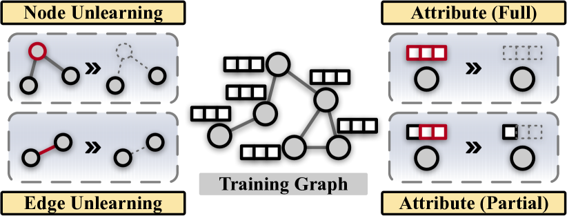
Figure 1. An illustration of common unlearning requests.

4. Methodology

In this section, we present our proposed framework IDEA, which aims to achieve flexible and certified unlearning for GNNs. We first present the general formulation of flexible unlearning for GNNs. Then, we introduce a unified modeling integrating different instantiations of unlearning requests. We finally propose a novel theoretical guarantee on the effectiveness of IDEA as the certification.

4.1. Flexible Unlearning for GNNs

We first present a unified formulation of flexible unlearning for GNNs. In general, our rationale here is to design a framework to directly approximate the change in the (optimal) learnable parameter $\bm{\theta}^{*}$ during unlearning. Specifically, we first review the training process of a given GNN model $f$ over graph data $\mathcal{G}$. Then, we consider the training objective with information of $\Delta\mathcal{G}$ being removed as a perturbed training objective over $\mathcal{G}$. We are now able to analyze how the optimal learnable parameter $\bm{\theta}^{*}$ would change when the objective function is modified. Note that we adopt a generalized formulation of such modification over the objective function, such that our analysis can be adapted to different unlearning requests.

In a typical training process of a given GNN model $f$ over graph data $\mathcal{G}$, the optimal learnable parameter $\bm{\theta}^{*}$ is obtained via solving the optimization problem of

(1) $$\arg\min_{\bm{\theta}}\frac{1}{m}\sum_{v_{i}\in\mathcal{V}_{\text{trn}}}\mathscr{L}\left(\bm{\theta},v_{i},\mathcal{G}\right),$$

where a typical choice of $\mathscr{L}$ is cross-entropy loss in node classification tasks. Here we consider that the computation of $\mathscr{L}$ also relies on other necessary information such as $\hat{Y}_{i}$ by default and omit them for simplicity. As a comparison, the optimal learnable parameter trained over $\mathcal{G}\ominus\Delta\mathcal{G}$, which we denoted as $\tilde{\bm{\theta}}^{*}$, is obtained via solving the problem of

(2) $$\arg\min_{\bm{\theta}}\frac{1}{m-|\Delta\mathcal{V}|}\sum_{v_{i}\in\mathcal{V}_{\text{trn}}\backslash\Delta\mathcal{V}}\mathscr{L}\left(\bm{\theta},v_{i},\mathcal{G}\ominus\Delta\mathcal{G}\right).$$

To study how the optimal parameters change when transforming from Equation (1) to Equation (2), it is necessary to analyze how the objective function and optimal solution change between the two cases. To systematically compare Equation (1) and Equation (2), here we define $\phi_{k}(\cdot)$ as a function that takes a node and a graph as its input and outputs the set of nodes in the computation graph of the input node (excluding the input node itself). Here a computation graph is a subgraph centered on a given node with neighboring nodes up to $k$ hops away, where $k$ is the layer number of the studied GNN. Then we have the following proposition.

Proposition 0.

Localized Equivalence of Training Nodes. Given $\Delta\mathcal{G}=\{\Delta\mathcal{V},\Delta\mathcal{E},\Delta\mathcal{X}\}$ to be unlearned and an objective $\mathscr{L}$ computed over $f_{\bm{\theta}}$, $\mathscr{L}\left(\bm{\theta},v_{i},\mathcal{G}\right)=\mathscr{L}\left(\bm{\theta},v_{i},\mathcal{G}\ominus\Delta\mathcal{G}\right)$ holds $\forall v_{i}\notin\phi_{k}(v_{j})\cup\{v_{j}\},v_{j}\in\Delta\mathcal{V}\cup\gamma_{e}(\Delta\mathcal{E})\cup\gamma_{x}(\Delta\mathcal{X})$. Here $\gamma_{e}$ and $\gamma_{x}$ return the set of nodes that directly connect to the edges in $\mathcal{E}$ and that have associated attribute(s) in $\mathcal{X}$, respectively.

The intuition of Proposition 1 is that, under a given $f_{\bm{\theta}}$, the value of $\mathscr{L}$ maintains the same between Equation (1) and Equation (2) for those training nodes that are not topologically close to the instances (i.e., nodes, attributes, and edges) in $\Delta\mathcal{G}$. To bridge Equation (1) and Equation (2), we then propose a formulation to characterize the intermediate state. Inspired by a series of previous works such as (Wu et al., 2023b, a), we add an additional term by defining $\bm{\theta}_{\Delta\mathcal{G},\xi}^{*}$ with

(3) $$\bm{\theta}_{\Delta\mathcal{G},\xi}^{*}\coloneqq\arg\min_{\bm{\theta}}\frac{1}{m}\sum_{v_{i}\in\mathcal{V}_{\text{trn}}}\mathscr{L}\left(\bm{\theta},v_{i},\mathcal{G}\right)+\xi\left(\mathscr{L}_{\text{add}}-\mathscr{L}_{\text{sub}}\right).$$

We then introduce the modeling of $\mathscr{L}_{\text{add}}$ and $\mathscr{L}_{\text{sub}}$. Specifically, we propose to formulate $\mathscr{L}_{\text{add}}$ with

$$\mathscr{L}_{\text{add}} =\alpha_{1}\sum_{v_{i}\in\mathcal{V}_{1}}\mathscr{L}\left(\bm{\theta},v_{i},\mathcal{G}\ominus\Delta\mathcal{G}\right)+\alpha_{2}\sum_{v_{i}\in\mathcal{V}_{2}}\mathscr{L}\left(\bm{\theta},v_{i},\mathcal{G}\ominus\Delta\mathcal{G}\right)$$

(4) $$+\alpha_{3} \sum_{v_{i}\in\mathcal{V}_{3}}\mathscr{L}\left(\bm{\theta},v_{i},\mathcal{G}\ominus\Delta\mathcal{G}\right)+\alpha_{4}\sum_{v_{i}\in\mathcal{V}_{4}}\mathscr{L}\left(\bm{\theta},v_{i},\mathcal{G}\ominus\Delta\mathcal{G}\right).$$

Here $\alpha_{1},\alpha_{2},\alpha_{3},\alpha_{4}\in\{0,1\}$ are used to flag whether the requests of node unlearning, full attribute unlearning, partial node attribute unlearning, and edge unlearning exist or not, respectively. We now introduce $\mathcal{V}_{1}$, $\mathcal{V}_{2}$, $\mathcal{V}_{3}$, and $\mathcal{V}_{4}$. Specifically, $\mathcal{V}_{1}$ represents the set of training nodes whose computation graph includes those nodes to be unlearned. We denote the sets of nodes associated with $\Delta\mathcal{X}$ when their unlearned attributes are replaced with any non-informative numbers (e.g., 0) as $\mathcal{V}_{x}^{\text{(Full)}}$ and $\mathcal{V}_{x}^{\text{(Partial)}}$ for full and partial attribute unlearning, respectively. $\mathcal{V}_{2}$ and $\mathcal{V}_{3}$ include training nodes whose computation graph includes attributes to be unlearned fully and partially plus the nodes in $\mathcal{V}_{x}^{\text{(Full)}}$ and $\mathcal{V}_{x}^{\text{(Partial)}}$, respectively; $\mathcal{V}_{4}$ is the set of nodes whose computation graph includes those edges to be unlearned. Mathematically, we formulate $\mathcal{V}_{1}$, $\mathcal{V}_{2}$, $\mathcal{V}_{3}$, and $\mathcal{V}_{4}$ as

(5) $$\mathcal{V}_{1} =\cup_{v_{i}\in\Delta\mathcal{V}}\left(\phi_{k}(v_{i})\cap\mathcal{V}_{\text{trn}}\right),$$

(6) $$\mathcal{V}_{2} =\mathcal{V}_{x}^{\text{(Full)}}\cup\{v_{i}:v_{i}\in\phi_{k}(v_{j})\cap\mathcal{V}_{\text{trn}},\;v_{j}\in\mathcal{V}_{x}^{\text{(Full)}}\},$$

(7) $$\mathcal{V}_{3} =\mathcal{V}_{x}^{\text{(Partial)}}\cup\{v_{i}:v_{i}\in\phi_{k}(v_{j})\cap\mathcal{V}_{\text{trn}},\;v_{j}\in\mathcal{V}_{x}^{\text{(Partial)}}\},$$

(8) $$\mathcal{V}_{4} =\cup_{v_{i}\in\gamma_{e}(\Delta\mathcal{E})}\left(\phi_{k}(v_{i})\cap\mathcal{V}_{\text{trn}}\right)$$

We then formulate $\mathscr{L}_{\text{sub}}$ as

$$\mathscr{L}_{\text{sub}}=\alpha_{1}\sum_{v_{i}\in\tilde{\mathcal{V}}_{1}}\mathscr{L}\left(\bm{\theta},v_{i},\mathcal{G}\right)+\alpha_{2}\sum_{v_{i}\in\tilde{\mathcal{V}}_{2}}\mathscr{L}\left(\bm{\theta},v_{i},\mathcal{G}\right)$$

(9) $$+\alpha_{3}\sum_{v_{i}\in\tilde{\mathcal{V}}_{3}}\mathscr{L}\left(\bm{\theta},v_{i},\mathcal{G}\right)+\alpha_{4}\sum_{v_{i}\in\tilde{\mathcal{V}}_{4}}\mathscr{L}\left(\bm{\theta},v_{i},\mathcal{G}\right),$$

where $\tilde{\mathcal{V}}_{1}$ includes all nodes in $\Delta\mathcal{V}$ and the training nodes within $k$ hops away from the nodes in $\Delta\mathcal{V}$; We denote the sets of nodes associated with $\Delta\mathcal{X}$ with their vanilla attributes as $\tilde{\mathcal{V}}_{x}^{\text{(Full)}}$ and $\tilde{\mathcal{V}}_{x}^{\text{(Partial)}}$ for full and partial attribute unlearning, respectively. $\tilde{\mathcal{V}}_{2}$ and $\tilde{\mathcal{V}}_{3}$ include training nodes whose computation graph includes attributes to be unlearned fully and partially plus the nodes in $\tilde{\mathcal{V}}_{x}^{\text{(Full)}}$ and $\tilde{\mathcal{V}}_{x}^{\text{(Partial)}}$, respectively; $\tilde{\mathcal{V}}_{4}$ is the set of nodes whose computation graph includes those edges to be unlearned, i.e., $\tilde{\mathcal{V}}_{4}=\mathcal{V}_{4}$. Mathematically, we have

(10) $$\tilde{\mathcal{V}}_{1} =\cup_{v_{i}\in\Delta\mathcal{V}}\left(\phi_{k}(v_{i})\cap\mathcal{V}_{\text{trn}}\right)\cup\Delta\mathcal{V},$$

(11) $$\tilde{\mathcal{V}}_{2} =\tilde{\mathcal{V}}_{x}^{\text{(Full)}}\cup\{v_{i}:v_{i}\in\phi_{k}(v_{j})\cap\mathcal{V}_{\text{trn}},\;v_{j}\in\tilde{\mathcal{V}}_{x}^{\text{(Full)}}\},$$

(12) $$\tilde{\mathcal{V}}_{3} =\tilde{\mathcal{V}}_{x}^{\text{(Partial)}}\cup\{v_{i}:v_{i}\in\phi_{k}(v_{j})\cap\mathcal{V}_{\text{trn}},\;v_{j}\in\tilde{\mathcal{V}}_{x}^{\text{(Partial)}}\},$$

(13) $$\tilde{\mathcal{V}}_{4} =\mathcal{V}_{4}.$$

We then have the complete formulation of Equation (3) given Equation (4.1) to (13). Based on the modeling above, we have the optimal equivalence between Equation (3) and Equation (2) below.

Lemma 0.

Optimal Equivalence. The optimal solution to Equation (3) (denoted as $\bm{\theta}_{\Delta\mathcal{G},\xi}^{*}$) equals to the optimal solution to Equation (2) (denoted as $\tilde{\bm{\theta}}^{*}$) when $\xi=\frac{1}{m}$.

Now we have successfully bridged the gap between Equation (1) and Equation (2) by modeling their intermediate states with Equation (3). More importantly, Lemma 2 paves the way towards directly approximating $\tilde{\bm{\theta}}^{*}$ based on $\bm{\theta}^{*}$ by giving Theorem 3 below.

Theorem 3.

Approximation with Infinitesimal Residual. Given a graph data $\mathcal{G}$, $\Delta\mathcal{G}=\{\Delta\mathcal{V},\Delta\mathcal{E},\Delta\mathcal{X}\}$ to be unlearned, and an objective $\mathscr{L}$ computed over an $f_{\bm{\theta}^{*}}$, using $\bm{\theta}^{*}+\frac{1}{m}\Delta\bar{\bm{\theta}}^{*}$ as an approximation of $\tilde{\bm{\theta}}^{*}$ only brings a first-order infinitesimal residual w.r.t. $\|\bm{\theta}^{*}-\tilde{\bm{\theta}}^{*}\|_{2}$, where $\Delta\bar{\bm{\theta}}^{*}=-\bm{H}^{-1}_{\bm{\theta}^{*}}\left(\nabla_{\bm{\theta}}\mathscr{L}_{\text{add}}-\nabla_{\bm{\theta}}\mathscr{L}_{\text{sub}}\right)$, and $\bm{H}_{\bm{\theta}^{*}}\coloneqq\nabla_{\bm{\theta}}^{2}\frac{1}{m}\sum_{v_{i}\in\mathcal{V}_{\text{trn}}}\mathscr{L}\left(\bm{\theta},v_{i},\mathcal{G}\right)$.

We note that the approximation strategy above relies on the assumption that $\forall\mathcal{V}_{i}\cap\mathcal{V}_{j}=\varnothing$ and $\forall\tilde{\mathcal{V}}_{i}\cap\tilde{\mathcal{V}}_{j}=\varnothing$ for $i,j\in\{1,2,3,4\}$ when $i\neq j$. However, it can also handle cases where such an assumption does not hold. We show this in Proposition 4.

Proposition 0.

Serializability of Approximation. Any mixture of unlearning request instantiations can be split into multiple sets of unlearning requests, where each set of unlearning requests satisfies $\forall\mathcal{V}_{i}\cap\mathcal{V}_{j}=\varnothing$ and $\forall\tilde{\mathcal{V}}_{i}\cap\tilde{\mathcal{V}}_{j}=\varnothing$ for $i,j\in\{1,2,3,4\}$ when $i\neq j$. Serially performing approximation following these request sets achieves upper-bounded error.

Unlearning in Practice. The approximation approach given by Theorem 3 requires computing the inverse matrix of the Hessian matrix, which usually leads to high computational costs. Here we propose to utilize the stochastic estimation method (Cook and Weisberg, 1980) to perform estimation based on an iterative approach, which reduces the time complexity to $O(tp)$. Here $t$ is the total number of iterations adopted by the stochastic estimation method, and $p$ represents the total number of learnable parameters in $\bm{\theta}$.

4.2. Unlearning Certification

In this subsection, we introduce a novel certification based on Theorem 3. According to the unlearning process given by Definition 1, our goal is to achieve guaranteed closeness between $\tilde{\bm{\theta}}^{*}$ (i.e., the ideal unlearned parameter derived from Equation (2)) and the approximation of such a parameter (denoted as $\bar{\bm{\theta}}^{*}$). In this way, we are able to achieve certifiable unlearning effectiveness.

Although certified unlearning for GNNs is studied by some recent explorations (Wu et al., 2023a; Chien et al., 2022b), these approaches can only be applied when the studied GNN model is trained following a specially modified objective. In particular, such a modification requires adding an additional regularization term of $\bm{\theta}$ scaled by a random vector onto the objective, which is specially designed for certification purposes. However, most GNNs are optimized following common objectives (e.g., cross-entropy loss) instead of such a modified objective. Therefore, these certified unlearning approaches cannot be flexibly used across different GNNs in real-world applications. Here we aim to develop a certified unlearning approach based on Theorem 3, such that it is not tailored for any optimization objective and thus can be easily generalized across various GNNs. Towards this goal, we first review the $\ell_{2}$ distances between $\bm{\theta}^{*}$, $\tilde{\bm{\theta}}^{*}$, and $\bar{\bm{\theta}}^{*}$. We present an illustration in Figure 2.

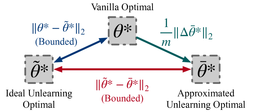
Figure 2. Distances between $\bm{\theta}^{*}$, $\tilde{\bm{\theta}}^{*}$, and $\bar{\bm{\theta}}^{*}$. Here, $\bm{\theta}^{*}$ denotes the optimal parameter before unlearning; $\tilde{\bm{\theta}}^{*}$ is the ideal optimal parameter after unlearning, which is obtained via re-training; $\bar{\bm{\theta}}^{*}$ is an approximation of $\tilde{\bm{\theta}}^{*}$ give by Theorem 3.

It is difficult to directly analyze the $\ell_{2}$ distance between $\tilde{\bm{\theta}}^{*}$ and $\bar{\bm{\theta}}^{*}$. We thus start by analyzing the $\ell_{2}$ distance between $\bm{\theta}^{*}$ and $\tilde{\bm{\theta}}^{*}$. We found that the $\ell_{2}$ distance between $\bm{\theta}^{*}$ and $\tilde{\bm{\theta}}^{*}$ is upper bounded under common assumptions, which are widely adopted in other existing works tackling unlearning problems (Wu et al., 2023a; Chien et al., 2022b; Guo et al., 2020). We first present these assumptions below.

Assumption 1.

For the training objective of a given GNN model, we have: (1) The loss values of optimal points are bounded: $|\mathscr{L}(\bm{\theta}^{*})|\leq C$ and $|\mathscr{L}(\tilde{\bm{\theta}}^{*})|\leq C$; (2) The loss function $\mathscr{L}$ is $L$-Lipschitz continuous; (3) The loss function $\mathscr{L}$ is $\lambda$-strongly convex.

Based on Assumption 1, we now present the bound between $\bm{\theta}^{*}$ and $\tilde{\bm{\theta}}^{*}$ in Theorem 5.

Theorem 5.

Distance Bound in Optimals. The $\ell_{2}$ distance bound between $\tilde{\bm{\theta}}^{*}$ and $\bm{\theta}^{*}$ is given by

(14) $$\|\tilde{\bm{\theta}}^{*}-\bm{\theta}^{*}\|_{2}\leq\frac{L|\Delta\mathcal{V}|+\sqrt{4m\lambda C|\tilde{\mathcal{V}}|+L^{2}|\Delta\mathcal{V}|^{2}}}{m\lambda}.$$

Denote $\mathcal{V}_{x}^{\text{(F+P)}}=\mathcal{V}_{x}^{\text{(Full)}}\cup\mathcal{V}_{x}^{\text{(Partial)}}$, and $\tilde{\mathcal{V}}$ is given by

(15) $$\tilde{\mathcal{V}}=\mathcal{V}_{1}\cup\mathcal{V}_{4}\cup\{v_{i}:v_{i}\in\phi_{k}(v_{j})\cap\mathcal{V}_{\text{trn}},\;v_{j}\in\mathcal{V}_{x}^{\text{(F+P)}}\}.$$

Here the rationale of $\tilde{\mathcal{V}}$ is to describe the set of nodes whose computation graphs involve any instance (i.e., nodes, attributes, and edges) to be unlearned. Noticing the relationship between $\bm{\theta}^{*}$, $\tilde{\bm{\theta}}^{*}$, and $\bar{\bm{\theta}}^{*}$ give by Figure 2, we further show the bound between $\tilde{\bm{\theta}}^{*}$ and $\bar{\bm{\theta}}^{*}$ in Proposition 6.

Proposition 0.

Distance Bound in Approximation. The $\ell_{2}$ distance bound between $\tilde{\bm{\theta}}^{*}$ and $\bar{\bm{\theta}}^{*}$ is given by

(16) $$\|\tilde{\bm{\theta}}^{*}-\bar{\bm{\theta}}^{*}\|_{2}\leq\frac{\lambda\|\Delta\bar{\bm{\theta}}^{*}\|_{2}+L|\Delta\mathcal{V}|+\sqrt{4m\lambda C|\tilde{\mathcal{V}}|+L^{2}|\Delta\mathcal{V}|^{2}}}{m\lambda}.$$

The rationale of Proposition 6 is to characterize the maximum $\ell_{2}$ distance between the ideal unlearning optimal and the approximation of unlearning optimal given by Theorem 3. Finally, based on Proposition 6, we are able to present the certification in Theorem 7.

Theorem 7.

Let $\bm{\theta}^{*}=\mathcal{A}\left(\mathcal{G}\right)$ be the empirical minimizer over $\mathcal{G}$, $\tilde{\bm{\theta}}^{*}=\mathcal{A}\left(\mathcal{G}\ominus\Delta\mathcal{G}\right)$ be the empirical minimizer over $\mathcal{G}\ominus\Delta\mathcal{G}$ and $\bar{\bm{\theta}}^{*}$ be an approximation of $\tilde{\bm{\theta}}^{*}$. Define $\zeta$ as an upper bound of $\|\tilde{\bm{\theta}}^{*}-\bar{\bm{\theta}}^{*}\|_{2}$. We have $\mathcal{U}\left(\mathcal{G},\Delta\mathcal{G},\mathcal{A}\left(\mathcal{G}\right)\right)=\bar{\bm{\theta}}^{*}+\bm{b}$ is an ($\varepsilon-\delta$) certified unlearning process, where $\bm{b}\sim\mathcal{N}(0,\sigma^{2}\bm{I})$ and $\sigma\geq\frac{\zeta}{\varepsilon}\sqrt{2\mathrm{ln(1.25/\delta)}}$.

Therefore, according to Theorem 7, we are able to achieve certified unlearning by adding zero-mean Gaussian noise over the approximation derived from Theorem 3.

5. Experimental Evaluations

We empirically evaluate the performance of IDEA in this section. In particular, we aim to answer the following research questions. RQ1: How tight can IDEA bound the $\ell_{2}$ distance between the ideal optimal $\tilde{\bm{\theta}}^{*}$ and the approximation $\bar{\bm{\theta}}^{*}$? RQ2: How well can IDEA improve the efficiency of unlearning compared with re-training and other alternatives? RQ3: How well can IDEA maintain the utility of the original GNN model? RQ4: How well can IDEA unlearn the information requested to be removed from the GNN?

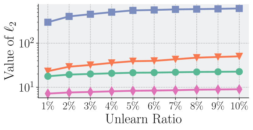
(a) Bounds vs. actual $\ell_{2}$ distance on Cora.

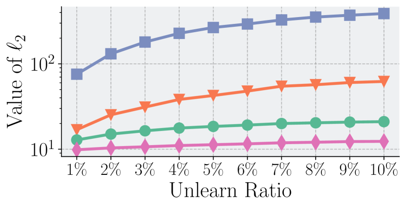
(b) Bounds vs. actual $\ell_{2}$ distance on Citeseer.

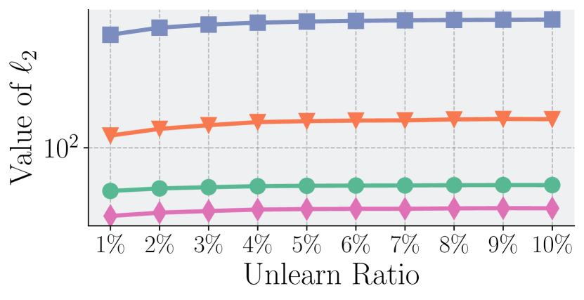
(c) Bounds vs. actual $\ell_{2}$ distance on PubMed.

Figure 3. Bounds and actual value of the $\ell_{2}$ distance between $\tilde{\bm{\theta}}^{*}$ and $\bar{\bm{\theta}}^{*}$, i.e., $\|\tilde{\bm{\theta}}^{*}-\bar{\bm{\theta}}^{*}\|_{2}$, over Cora, CiteSeer and PubMed datasets. CEU Worst, CEU Data Dependent, IDEA, and Actual represent the worst bound based on CEU, the data-dependent bound based on CEU, the bound based on IDEA, and the actual value of $\|\tilde{\bm{\theta}}^{*}-\bar{\bm{\theta}}^{*}\|_{2}$ derived from re-training, respectively.

5.1. Experimental Setup

Downstream Task and Datasets. We adopt the widely studied node classification task as the downstream task, which accounts for a wide range of real-world applications based on GNNs. We perform experiments over five real-world datasets, including Cora (Kipf and Welling, 2017), Citeseer (Kipf and Welling, 2017), PubMed (Kipf and Welling, 2017), Coauthor-CS (Shchur et al., 2018; Chen et al., 2022), and Coauthor-Physics (Shchur et al., 2018; Chen et al., 2022). These datasets usually serve as commonly used benchmark datasets for GNN performance over node classification tasks. Specifically, Cora, Citeseer, and PubMed are citation networks, where nodes denote research publications and edges represent the citation relationship between any pair of publications. The node attributes are bag-of-words representations of the publication keywords. Coauthor-CS, and Coauthor-Physics are two coauthor networks, where nodes represent authors and edges denote the collaboration relationship between any pair of authors. We leave more dataset details, e.g., their statistics, in Appendix.

Backbone GNNs. To evaluate the generalization ability of IDEA across different GNNs, we propose to utilize two types of GNNs, including linear and non-linear GNNs. In terms of linear GNNs, we adopt the popular SGC (Wu et al., 2019a); in terms of non-linear GNNs, we adopt three popular ones, including GCN (Kipf and Welling, 2017), GAT (Veličković et al., 2017), and GIN (Xu et al., 2019).

Unlearning Requests. We consider all unlearning requests presented in Section 3. For each type of request, we perform experiments over a wide range of scales in terms of the number of unlearned instances (e.g., nodes and edges). For experiments with fixed ratios, we adopt a ratio of 5% to perform unlearning for nodes or edges unless otherwise specified.

Threat Models. To evaluate the effectiveness of the unlearning strategy, we propose to adopt different types of threat models. Although IDEA is able to flexibly perform four different types of unlearning requests, there are only limited threat models can be chosen from. In our experiments, we adopt two state-of-the-art threat models, namely MIA-Graph (Olatunji et al., 2021) and StealLink (He et al., 2021), for node membership inference attack and link stealing attack, respectively.

Baselines. We adopt five types of baselines for performance comparison. (1) Re-Training. We adopt the re-training approach to obtain an ideal model based on the optimization problem given by Equation (2). (2) Exact Unlearning. We adopt the popular GraphEraser (Chen et al., 2022) as a representative method for exact unlearning. Specifically, exact unlearning methods aim to achieve the exact same probability distribution in the model space (after unlearning) compared with the re-trained model. As a comparison, IDEA aims to approximate the distribution of the re-trained model through unlearning. (3) Certified Unlearning. Finally, we adopt two representative approaches for certified unlearning, namely Certified Graph Unlearning (CGU) (Chien et al., 2022a) and Certified Edge Unlearning (CEU) (Wu et al., 2023a). CGU is able to unlearn nodes, attributes, and edges. However, it is only applicable for the SGC model. As a comparison, CEU can be adapted to different GNNs. Nevertheless, it is specially designed for edge unlearning.

Evaluation Metrics. We evaluate IDEA with different metrics to answer the four research questions. (1) Bound Tightness. We propose to compare the numerical values of the bounds given by IDEA, the bounds given by other baselines, and the actual $\ell_{2}$ distance of model parameters yielded by re-training. A smaller bound on the $\ell_{2}$ distance indicates better tightness. (2) Model Utility. We utilize the F1 score to measure the model utility after unlearning. A higher F1 score indicates better performance. (3) Unlearning Efficiency. We utilize the running time (in seconds) that the unlearning methods take to measure efficiency, and a shorter running time indicates better efficiency. (4) Unlearning Effectiveness. We use the attack successful rate after unlearning to measure unlearning effectiveness. Lower attack successful rates indicate better effectiveness.

Table 1. F1 score on five real-world graph datasets under node classification task. All numerical values are reported in percentage, and the F1 scores given by the proposed framework IDEA are marked in bold.

		Cora	CiteSeer	PubMed	CS	Physics
GCN	Re-Training	76.88 $\pm$ 0.3	67.27 $\pm$ 0.6	76.20 $\pm$ 0.0	86.79 $\pm$ 0.3	92.30 $\pm$ 0.0
	Random	47.97 $\pm$ 0.5	46.25 $\pm$ 5.6	70.98 $\pm$ 0.1	80.64 $\pm$ 0.3	75.23 $\pm$ 0.1
	BEKM	50.68 $\pm$ 2.0	46.85 $\pm$ 4.9	69.64 $\pm$ 0.1	80.30 $\pm$ 0.2	74.85 $\pm$ 0.1
	BLPA	43.79 $\pm$ 2.2	40.24 $\pm$ 8.3	63.42 $\pm$ 5.7	85.10 $\pm$ 0.3	78.93 $\pm$ 0.5
	IDEA	72.08 $\pm$ 1.2	61.56 $\pm$ 1.2	73.11 $\pm$ 0.0	86.13 $\pm$ 0.4	91.93 $\pm$ 0.1
SGC	Re-Training	76.14 $\pm$ 0.6	65.77 $\pm$ 0.0	75.90 $\pm$ 0.0	87.10 $\pm$ 0.1	92.01 $\pm$ 0.0
	Random	46.00 $\pm$ 0.7	45.25 $\pm$ 3.0	69.03 $\pm$ 0.1	81.30 $\pm$ 0.3	80.81 $\pm$ 0.1
	BEKM	48.83 $\pm$ 1.8	46.45 $\pm$ 0.4	69.76 $\pm$ 0.1	80.08 $\pm$ 0.2	74.87 $\pm$ 0.2
	BLPA	63.59 $\pm$ 1.4	39.44 $\pm$ 2.8	62.98 $\pm$ 4.6	86.95 $\pm$ 0.1	87.38 $\pm$ 0.1
	IDEA	72.94 $\pm$ 1.9	63.16 $\pm$ 1.0	73.63 $\pm$ 0.8	84.68 $\pm$ 0.3	91.21 $\pm$ 0.1
GIN	Re-Training	82.90 $\pm$ 0.6	74.27 $\pm$ 0.5	85.31 $\pm$ 0.6	90.28 $\pm$ 0.2	95.57 $\pm$ 0.2
	Random	69.25 $\pm$ 6.3	51.85 $\pm$ 2.7	83.64 $\pm$ 1.2	89.17 $\pm$ 0.1	91.74 $\pm$ 0.5
	BEKM	74.05 $\pm$ 3.5	65.17 $\pm$ 2.8	84.35 $\pm$ 0.3	89.39 $\pm$ 0.5	92.30 $\pm$ 0.3
	BLPA	62.48 $\pm$ 2.9	55.06 $\pm$ 7.2	82.25 $\pm$ 1.6	62.29 $\pm$ 0.7	71.66 $\pm$ 1.4
	IDEA	72.57 $\pm$ 2.8	66.37 $\pm$ 4.6	82.33 $\pm$ 0.2	88.48 $\pm$ 0.6	94.63 $\pm$ 0.1
GAT	Re-Training	83.76 $\pm$ 0.3	75.88 $\pm$ 0.1	85.02 $\pm$ 0.1	92.24 $\pm$ 0.1	95.28 $\pm$ 0.1
	Random	58.18 $\pm$ 2.0	55.43 $\pm$ 4.3	68.20 $\pm$ 6.9	80.75 $\pm$ 0.1	78.26 $\pm$ 0.1
	BEKM	64.20 $\pm$ 1.5	57.35 $\pm$ 2.8	71.67 $\pm$ 0.2	80.37 $\pm$ 0.3	77.47 $\pm$ 0.2
	BLPA	60.88 $\pm$ 1.0	58.26 $\pm$ 2.6	67.34 $\pm$ 3.4	85.22 $\pm$ 0.2	86.12 $\pm$ 0.2
	IDEA	84.38 $\pm$ 0.6	75.78 $\pm$ 0.9	84.92 $\pm$ 0.2	92.20 $\pm$ 0.2	95.41 $\pm$ 0.0

5.2. Evaluation of Bound Tightness

To answer RQ1, we first evaluate how tight the derived bound between $\tilde{\bm{\theta}}^{*}$ and $\bar{\bm{\theta}}^{*}$ can be across different GNNs, graph datasets, and unlearning ratios. We also compare the bound derived based on IDEA and other bounds in existing works. To the best of our knowledge, CEU (Wu et al., 2023a) is the only existing certified unlearning approach that provides generalizable bounds across different GNNs. In particular, CEU provides bounds over the objective function after unlearning, and we adapt such bounds over the objective function to $\ell_{2}$ distance bounds between $\tilde{\bm{\theta}}^{*}$ and $\bar{\bm{\theta}}^{*}$ based on the common assumption of the objective function being Lipschitz continuous (Wu et al., 2023a). We compare the bounds and the $\ell_{2}$ distances below. (1) CEU Worst Bound. We compute the theoretical worst bound derived based on CEU as a baseline of the $\ell_{2}$ distance bound between $\tilde{\bm{\theta}}^{*}$ and $\bar{\bm{\theta}}^{*}$. (2) CEU Data-Dependent Bound. We compute the data-dependent bound derived based on CEU as a baseline of the $\ell_{2}$ distance bound between $\tilde{\bm{\theta}}^{*}$ and $\bar{\bm{\theta}}^{*}$. A data-dependent bound is tighter than the Worst Bound. (3) IDEA Bound. We compute the bound given by Proposition 6 as the bound for the $\ell_{2}$ distance between $\tilde{\bm{\theta}}^{*}$ and $\bar{\bm{\theta}}^{*}$. (4) Actual Values. We compare the bounds above with the actual $\ell_{2}$ distance between $\tilde{\bm{\theta}}^{*}$ and $\bar{\bm{\theta}}^{*}$. Note that we focus on edge unlearning tasks to analyze the tightness of the derived bounds, since this is the only unlearning task CEU supports. We use Unlearn Ratio to refer to the ratio of edges to be unlearned from the GNN.

We present the bounds and the actual value of the $\ell_{2}$ distance between $\tilde{\bm{\theta}}^{*}$ and $\bar{\bm{\theta}}^{*}$ over a wide range of unlearn ratios (from 1% to 10%), which covers common values, in Figure 3. We also have similar observations in other cases (see Appendix). We summarize the observations below. (1) From the perspective of the general tendency, we observe that larger unlearn ratios usually lead to larger values in both the derived bounds and the actual $\ell_{2}$ distance between $\tilde{\bm{\theta}}^{*}$ and $\bar{\bm{\theta}}^{*}$. This reveals that a larger unlearn ratio tends to make the approximation of $\tilde{\bm{\theta}}^{*}$ (with the calculated $\bar{\bm{\theta}}^{*}$) more difficult, which is in alignment with existing works (Wu et al., 2023a). (2) From the perspective of the bound tightness, we found that IDEA is able to give tighter bounds in all cases compared with the bounds given by CEU, especially in cases with larger unlearn ratios. This reveals that the approximation of $\tilde{\bm{\theta}}^{*}$ given by IDEA can better characterize the difference between $\tilde{\bm{\theta}}^{*}$ and $\bm{\theta}^{*}$ compared with CEU.

5.3. Evaluation of Unlearning Efficiency

To answer RQ2, we then evaluate the efficiency of IDEA in performing unlearning. Specifically, we adopt the common node unlearning task as an example, and we measure the running time of unlearning in seconds. We note that CGU only supports performing unlearning on SGC, and thus we adopt SGC as the backbone GNN for IDEA and all other baselines for a fair comparison. We use Unlearn Ratio to refer to the ratio of training nodes to be unlearned from the GNN. Here we present a comparison between IDEA and baselines on Cora dataset in Figure 4. We also have similar observations on other GNNs and datasets (see Appendix). We summarize the observations below. (1) From the perspective of the general tendency, we observe that the running time of re-training does not change across different unlearning ratios. This is because the number of optimization epochs dominates the running time of re-training, while the total epoch number does not change no matter how many training nodes are removed. However, the efficiency of all other baselines is sensitive to the unlearning ratio, and this is because their running time is closely dependent on the total number of nodes to be unlearned. Finally, we found that the running time of IDEA is not sensitive to the unlearn ratio. This is because the number of nodes to be unlearned will only marginally influence the computational costs associated with Theorem 3. The stable running time across different numbers of nodes to be unlearned serves as a key superiority of IDEA over other baselines. (2) From the perspective of time comparison, we found that IDEA achieves significant superiority over all other baselines across the wide range of unlearning ratios, especially on relatively large ones (e.g., 10%). Such an observation indicates that IDEA is able to perform unlearning with satisfying efficiency, which further reveals its practical significance in real-world applications.

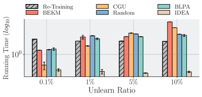
Figure 4. Efficiency comparison between IDEA and other baselines including retraining. Running time is measured with seconds and presented in log scale.

5.4. Evaluation of Model Utility

To answer RQ3, we now compare model utility after performing unlearning with IDEA and other baselines. We note that GraphEraser is the only baseline that supports flexible generalization across different GNN backbones. Therefore, we adopt the three variants of GraphEraser, i.e., Random, BEKM, and BLPA, as the corresponding baselines for comparison. We adopt the most common task of node unlearning, and we adopt the F1 score (of node classification) to measure the model utility after re-training/unlearning. We present comprehensive empirical results (including four different GNN backbones and all five real-world datasets) in Table 1. In addition to the baselines, we also report the performance of re-training, i.e., the F1 score given by a re-trained model with the unlearned nodes being removed from the training graph, for comparison. We summarize the observations below, and similar observations are also found in different settings (see Appendix). (1) From the perspective of the general tendency, we observe that unlearning approaches are usually associated with worse utility performance compared with re-training. Such a sacrifice is usually considered acceptable, since these unlearning approaches can bring significant improvement in efficiency compared with re-training. (2) From the perspective of model utility, we found that IDEA achieves competitive utility compared with other baselines. Specifically, compared with re-training, IDEA only sacrifices limited utility performance in most cases, and even shows better performance in certain cases. Furthermore, compared with other alternatives, IDEA also shows consistent superiority in most cases.

5.5. Evaluation of Unlearning Effectiveness

To answer RQ4, we compare the unlearning effectiveness of IDEA and other baselines. Specifically, we utilize the state-of-the-art attack methods MIA-Graph and StealLink to evaluate the unlearning effectiveness of node and edge unlearning tasks, respectively. To also have CGU as a baseline, we adopt SGC as the backbone GNN to ensure a fair comparison. We present the attack successful rates after node and edge unlearning in Table 2. All attacks are performed over those unlearned nodes/edges, and thus a lower AUC score represents better unlearning performance. In terms of node attributes unlearning, we note that to the best of our knowledge, no existing membership inference attack method supports the associated attack. Here we use the average loss value as an unlearning performance indicator. Specifically, we perform partial attribute unlearning under different ratios (20%, 50%, 80%) of unlearn attribute dimensions to the total attribute dimensions. Note that partial attribute unlearning aims to twist the GNN model such that the GNN model behaves as if it were trained on those nodes with the unlearn attribute values being set to non-informative numbers (as in Section 3). Here we follow a common choice (Chien et al., 2022a) to set such a number as zero. Accordingly, we evaluate the performance with the average loss values regarding the nodes with the unlearn attributes being set to zeros, and a lower loss value indicates better unlearning effectiveness. We present the results in Table 3. Note that CGU only supports full attribute unlearning, while the three variants of GraphEraser only support node/edge unlearning. Therefore, we perform attribute unlearning and node unlearning for CGU and GraphEraser, respectively. Based on the settings above, we have the observations below, and consistent observations are also found under different settings (see Appendix). (1) From the perspective of node and edge unlearning, we observe that the attack AUC scores over IDEA are among the lowest in both unlearning tasks. Noticing that the AUC scores given by IDEA are only marginally above 50%, the unlearned node/edge information has been almost completely removed from the trained GNNs. (2) From the perspective of attribute unlearning, IDEA exhibits the lowest average loss values in all (attribute) unlearn ratios. This indicates the superior attribute unlearning performance.

Table 2. Attack AUC scores after node and edge unlearning on Cora. The results given by IDEA are marked in bold.

	Node Unlearning ($\downarrow$)	Edge Unlearning ($\downarrow$)
Random	50.38 $\pm$ 0.5	55.64 $\pm$ 2.8
BEKM	50.35 $\pm$ 1.2	51.81 $\pm$ 0.3
BLPA	50.30 $\pm$ 0.4	50.84 $\pm$ 3.4
CGU	54.67 $\pm$ 2.9	66.52 $\pm$ 0.6
IDEA	50.86 $\pm$ 1.8	50.11 $\pm$ 0.9

Table 3. Average loss values on Cora regarding the nodes with the unlearn attributes being set to zeros. Ratio of unlearn node attribute dimensions to all attribute dimensions varies across 20%, 50%, and 80%. Lower values represent better performance, and results from IDEA are marked in bold.

	20% ($\downarrow$)	50% ($\downarrow$)	80% ($\downarrow$)
Random	1.32 $\pm$ 0.06	1.38 $\pm$ 0.06	1.35 $\pm$ 0.09
BEKM	1.41 $\pm$ 0.16	1.47 $\pm$ 0.14	1.39 $\pm$ 0.12
BLPA	1.47 $\pm$ 0.11	1.69 $\pm$ 0.37	1.50 $\pm$ 0.05
CGU	1.62 $\pm$ 0.02	1.73 $\pm$ 0.04	1.78 $\pm$ 0.06
IDEA	1.29 $\pm$ 0.01	1.31 $\pm$ 0.01	1.33 $\pm$ 0.01

6. Related Work

Certified Machine Unlearning. The general desiderata of machine unlearning is to remove the influence of certain training data on the model parameters, such that the model can behave as if it never saw such data (Xu et al., 2023b; Nguyen et al., 2022; Bourtoule et al., 2021; Yan et al., 2022; Wang et al., 2024; Grimes et al., 2024). Re-training the model without making the unlearning data visible is an ideal way to achieve such a goal, while it is usually infeasible in practice due to various reasons such as prohibitively high computational costs (Zhang et al., 2023b; Xu et al., 2024; Qu et al., 2023; Schelter et al., 2023). A popular way to approach the goal of unlearning is to directly approximate the re-trained model parameters, a.k.a., approximate unlearning (Xu et al., 2023b; Thudi et al., 2022). Certified machine unlearning is under the umbrella of approximate unlearning (Liu et al., 2024b; Zhang et al., 2023c), and it has stood out due to the capability of providing theoretical guarantee on the unlearning effectiveness. A commonly used criterion of certified unlearning is $(\varepsilon-\delta)$ certified unlearning (Guo et al., 2019; Sekhari et al., 2021; Liu et al., 2024a; Dai et al., 2022), which utilizes two parameters $\varepsilon$ and $\delta$ to describe the proximity between the re-trained model parameter distribution and approximated model parameter distribution in the model space. In recent years, various techniques have been proposed to achieve certified unlearning (Zhang et al., 2022; Warnecke et al., 2021; Mahadevan and Mathioudakis, 2021). However, they overwhelmingly focus on independent, identically distributed (i.i.d.) data and fail to consider the dependency between data points. Therefore, they cannot be directly adopted to perform unlearning over GNNs (Wu et al., 2023b, a). Different from the works mentioned above, our paper proposes a certified unlearning approach for GNNs, necessitating the modeling of dependencies between instances in graphs (e.g., nodes and edges).

Machine Unlearning for Graph Neural Networks. Over the years, GNNs have been increasingly deployed in a plethora of applications (Zhou et al., 2020; Wu et al., 2022; Neo et al., 2024; Jin et al., 2023; Ma et al., 2022; Shi et al., 2023; Dong et al., 2023b; Zhang et al., 2023a; Dong et al., 2023a). Similar to other machine learning models, these GNN models also face the risk of privacy leakage (Qiu et al., 2022; Shan et al., 2021; Ju et al., 2024; Sajadmanesh, 2023; Wang et al., 2023; Xu et al., 2023a), where the private information is usually considered to be encoded in the training data (Said et al., 2023). Such a threat has prompted the emerging of unlearning approaches for GNNs (Chen et al., 2022; Pan et al., 2023; Cheng et al., 2023; Wu et al., 2023b). However, these works are only able to achieve unlearning for GNNs empirically, failing to provide any theoretical guarantee on the effectiveness. To further strengthen the power of unlearning for GNNs and enhance the confidence of model owners before model deployment, a few recent works have initiated explorations on certified unlearning for GNNs. Wu et al. (Wu et al., 2023a) propose CEU to unlearn edges that are visible to GNNs during training, while edge unlearning is the only type of request it is able to handle. Chien et al. (Chien et al., 2022a) proposed a different certified unlearning approach for GNNs to also handle node and attribute unlearning requests, while such an approach is only applicable to a specially simplified GNN model. Meanwhile, these approaches can only handle limited types of unlearning requests, which further jeopardizes their flexibility in real-world applications. Different from them, our paper proposes a flexible unlearning framework that can handle different types of unlearning requests. On top of this framework, an effectiveness certification is further proposed without relying on any specific GNN structure or objective function.

7. Conclusion

In this paper, we propose IDEA, a flexible framework of certified unlearning for GNNs. Specifically, we first formulate and study a novel problem of flexible and certified unlearning for GNNs, which aims to flexibly handle different unlearning requests with theoretical guarantee. To tackle this problem, we develop IDEA by analyzing the objective difference before and after certain information is removed from the graph. We further present theoretical guarantee as the certification for unlearning effectiveness. Extensive experiments on real-world datasets demonstrate the superiority of IDEA in multiple key perspectives. Meanwhile, two future directions are worth further investigation. First, we focus on the common node classification task in this paper, and we will extend the proposed framework to other tasks, such as graph classification. Second, considering that GNNs may be trained in a decentralized manner, it is critical to study GNN unlearning under a distributed setting.

8. Acknowledgements

This work is supported in part by the National Science Foundation under IIS-2006844, IIS-2144209, IIS-2223769, IIS-1900990, IIS-2239257, IIS-2310262, CNS-2154962, and BCS-2228534; the Commonwealth Cyber Initiative Awards under VV-1Q23-007, HV-2Q23-003, and VV-1Q24-011; the JP Morgan Chase Faculty Research Award; the Cisco Faculty Research Award; and Snap gift funding.

Appendix A Reproducibility

In this section, we introduce the details of the experiments in this paper for the purpose of reproducibility. At the same time, we have uploaded all necessary code to our GitHub repository to reproduce the results presented in this paper: https://github.com/yushundong/IDEA. All major experiments are encapsulated as shell scripts, which can be conveniently executed. We introduce details in the subsections below.

A.1. Real-World Datasets.

Here we briefly introduce the five real-world graph datasets we used in this paper, and all these datasets are commonly used datasets in node classification tasks. We present their statistics in Table 4.

A.2. Experimental Settings.

For all datasets, we follow a commonly used split (Wu et al., 2023b) of 90% and 10% for training and test node set, respectively. In the task of node classification, only the node labels in the training set are visible for all models during the training process. We adopt a learning rate of 0.01 for most models in our experiments, including the backbone GNNs in the proposed framework IDEA, together with commonly used number of epochs, e.g., 300. The value of the standard deviation adopted by IDEA falls into the range of (1e-3, 1e0), and the values are consistent in different experiments for each unlearning task.

A.3. Implementation of IDEA.

IDEA is implemented based on PyTorch (Paszke et al., 2017) and optimized through Adam optimizer (Kingma and Ba, 2014). In experiments, IDEA and other unlearning baselines require assumption on the characteristics regarding the objective function. We set all these values to be commonly used values in existing works focusing on machine unlearning, and these values are set to be consistent across all methods for the purpose of fair comparison. Here we present the specific values we adopted. Specifically, the objective function is assumed to be 0.05 strongly-convex, and the Lipschitz constant of the objective function is set to be 0.25. The numerical bound of the training loss regarding each training nodes is set to be 3.0 around the optimal point, which can be easily satisfied in practice. In addition, the Lipschitz constant of the Hessian matrix of the objective function is assumed to be 0.25. The derivative of the objective function is set to be bounded by 1.0, and the Lipschitz constant of the first-order derivative of the objective function is also set to be 1.0.

A.4. Implementation of Graph Neural Networks.

For all adopted GNNs (i.e., SGC, GCN, GAT, and GIN) in our experiments, their released implementations are utilized for a fair comparison. The layer number for GCN and GIN is set as two. We adopt a dropout rate as 0.6, and the attention head number of GAT is set as eight. Meanwhile, we note that same observations can also be found under different settings.

Table 4. Statistics of the adopted real-world graph datasets.

	#Nodes	#Edges	#Attributes	#Classes
Cora	2,708	5,429	1,433	7
CiteSeer	3,327	4,723	3,703	6
PubMed	19,717	88,648	500	3
CS	18,333	163,788	6,805	15
Physics	34,493	495,924	8,415	5

A.5. Implementation of Baselines.

Re-Training. We adopt re-training as our first baseline for performance comparison. Note that the randomness in initialization and optimization may significantly influence the performance. Hence we continue to train the optimized GNN model with the unlearning instances (e.g., nodes and edges to be unlearned) being removed, and consider this model as the re-trained model. Such a strategy is also widely used in other works (e.g., (Koh and Liang, 2017)) based on influence function and their main goal remains consistent with us, i.e., to avoid the randomness induced by initialization and optimization.

Graph Unlearning (GraphEraser). We adopt GraphEraser as another baseline for comparison. In total, GraphEraser has three types of variants (including Random, BEKM, BLPA), which are all adopted in our paper for comparison. These variants associates with different types of graph partition methods. In addition, we follow their reported results to adopt LBAggr as the aggregator in GraphEraser to achieve its best performance in model utility. We adopt its official open-source code for experiments.

Certified Graph Unlearning (CGU). We adopt CGU as another baseline for comparison. We note that CGU only supports SGC as the corresponding GNN backbone model. We adopt its official open-source code for experiments.

Certified Edge Unlearning (CEU). We also adopt CEU as a baseline for comparison. We note that CEU only supports edge unlearning as the corresponding unlearning task. We adopt its official open-source code for experiments.

A.6. Implementation of Threat Models.

MIA-Graph. We adopt MIA-Graph as the node attack method. We note that since MIA-Graph has several variants that might influence attack efficacy, we select the attack strategy with the best empirical performance, which entails training a shadow model using the original dataset’s ground truth labels. Then we employ the output class posterior probabilities of the shadow model to train an attack model, which is later deployed to execute attacks on the target model with unlearned instances. To compute the successful rate, we select all the unlearned instances as positive samples, and an equal number of instances at random from the target model’s test set as negative samples. We adopt the official code for experiments.

StealLink. We adopt StealLink as the edge attack method. Note that StealLink integrates multiple attack strategies each necessitating different background knowledge. Here we choose attack-3 from the original paper, wherein the adversary has access to a partial graph of the target datasets, due to its high successful rate in attacks. Here we select a partial graph size equivalent to $50\%$ of all edges to train the attack model, where the output class posterior probabilities are utilized as features. To compute the successful rate, we select all the unlearned edges as positive samples, and an equal number of instances at random from the edges that do not exist in the original dataset. We adopt official open-source code for experiments.

A.7. Packages Required for Implementations.

We perform the experiments on a server with multiple Nvidia A6000 GPUs. Below we list the key packages and their associated versions in our implementation.

• Python == 3.8.8

• torch == 1.10.1+cu111

• torch-cluster == 1.6.0

• torch-geometric == 2.2.0

• torch-scatter == 2.0.9

• torch-sparse == 0.6.13

• cuda == 11.1

• numpy == 1.20.1

• tensorboard == 1.13.1

• networkx == 2.5

• scikit-learn==0.24.2

• pandas==1.2.4

• scipy==1.6.2

Appendix B Proofs

Proposition 1.

Localized Equivalence of Training Nodes. Given $\Delta\mathcal{G}=\{\Delta\mathcal{V},\Delta\mathcal{E},\Delta\mathcal{X}\}$ to be unlearned ($v_{i}\notin\Delta\mathcal{V}$) and an objective $\mathscr{L}$ computed over $f_{\bm{\theta}}$, $\mathscr{L}\left(\bm{\theta},v_{i},\mathcal{G}\right)=\mathscr{L}\left(\bm{\theta},v_{i},\mathcal{G}\ominus\Delta\mathcal{G}\right)$ holds $\forall v_{i}\notin\phi_{k}(v_{j})\cup\{v_{j}\},v_{j}\in\Delta\mathcal{V}\cup\gamma_{e}(\Delta\mathcal{E})\cup\gamma_{x}(\Delta\mathcal{X})$. Here $\gamma_{e}$ and $\gamma_{x}$ return the set of nodes that directly connect to the edges in $\mathcal{E}$ and that have associated attribute(s) in $\mathcal{X}$, respectively.

Proof.

For most GNNs based on message passing, the embedding of a node is only determined by its $k$-hop neighbors (Hamilton et al., 2017). For each layer in the GNN, each node can be seen as aggregating the embeddings of its one-hop neighbors. For any $v_{j}\in\Delta\mathcal{V}$, $v_{i}\notin\phi_{k}(v_{j})$ and we have $v_{j}\notin\phi_{k}(v_{i})$. Consequently, we have $\mathscr{L}\left(\bm{\theta},v_{i},\mathcal{G}\right)=\mathscr{L}\left(\bm{\theta},v_{i},\mathcal{G}\ominus\Delta\mathcal{G}\right)$. ∎

Lemma 1.

Optimal Equivalence. The optimal solution to Equation (3) (denoted as $\bm{\theta}_{\Delta\mathcal{G},\xi}^{*}$) equals to the optimal solution to Equation (2) (denoted as $\tilde{\bm{\theta}}^{*}$) when $\xi=\frac{1}{m}$.

Proof.

Incorporate Section 4.1 and Section 4.1 into Equation 3, we come to

(17) $$\bm{\theta}_{\Delta\mathcal{G},\xi}^{*} =\arg\min_{\bm{\theta}}\frac{1}{m}\sum_{v_{i}\in\mathcal{V}_{\text{trn}}}\mathscr{L}\left(\bm{\theta},v_{i},\mathcal{G}\right)+\xi\left(\mathscr{L}_{\text{add}}-\mathscr{L}_{\text{sub}}\right)$$

$$=\arg\min_{\bm{\theta}}\frac{1}{m}\sum_{v_{i}\in\mathcal{V}_{\text{trn}}}\mathscr{L}\left(\bm{\theta},v_{i},\mathcal{G}\right)$$

$$+\xi\left(\sum_{v_{i}\in\mathcal{V}_{\text{trn}}\backslash\Delta\mathcal{V}}\mathscr{L}\left(\bm{\theta},v_{i},\mathcal{G}\ominus\Delta\mathcal{G}\right)-\sum_{v_{i}\in\mathcal{V}_{\text{trn}}}\mathscr{L}\left(\bm{\theta},v_{i},\mathcal{G}\right)\right).$$

When $\xi=\frac{1}{m}$, we consequently have

(18) $$\bm{\theta}_{\Delta\mathcal{G},\xi}^{*}=\arg\min_{\bm{\theta}}\frac{1}{m}\sum_{v_{i}\in\mathcal{V}_{\text{trn}}\backslash\Delta\mathcal{V}}\mathscr{L}\left(\bm{\theta},v_{i},\mathcal{G}\ominus\Delta\mathcal{G}\right)=\tilde{\bm{\theta}}^{*},$$

which finishes our proof. ∎

Theorem 1.

Approximation with Infinitesimal Residual. Given a graph data $\mathcal{G}$, $\Delta\mathcal{G}=\{\Delta\mathcal{V},\Delta\mathcal{E},\Delta\mathcal{X}\}$ to be unlearned, and an objective $\mathscr{L}$ computed over an $f_{\bm{\theta}^{*}}$, using $\bm{\theta}^{*}+\frac{1}{m}\Delta\bar{\bm{\theta}}^{*}$ as an approximation of $\tilde{\bm{\theta}}^{*}$ only brings a first-order infinitesimal residual w.r.t. $\|\bm{\theta}^{*}-\tilde{\bm{\theta}}^{*}\|_{2}$, where $\Delta\bar{\bm{\theta}}^{*}=-\bm{H}^{-1}_{\bm{\theta}^{*}}\left(\nabla_{\bm{\theta}}\mathscr{L}_{\text{add}}-\nabla_{\bm{\theta}}\mathscr{L}_{\text{sub}}\right)$, and $\bm{H}_{\bm{\theta}^{*}}\coloneqq\nabla_{\bm{\theta}}^{2}\frac{1}{m}\sum_{v_{i}\in\mathcal{V}_{\text{trn}}}\mathscr{L}\left(\bm{\theta},v_{i},\mathcal{G}\right)$.

Proof.

For simplicity, we define the function $\Phi(\cdot)$ as $\Phi(\bm{\theta})=\frac{1}{m}\sum_{v_{i}\in\mathcal{V}_{\text{trn}}}\mathscr{L}\left(\bm{\theta},v_{i},\mathcal{G}\right)+\xi\left(\mathscr{L}_{\text{add}}-\mathscr{L}_{\text{sub}}\right)$. We then conduct the Taylor expansion of $\nabla_{\bm{\theta}}\Phi(\bm{\theta})$ at $\bm{\theta}=\bm{\theta}^{*}$ as

(19) $$\nabla_{\bm{\theta}}\Phi(\bm{\theta})=\nabla_{\bm{\theta}}\Phi(\bm{\theta}^{*})+\nabla^{2}_{\bm{\theta}}\Phi(\bm{\theta}^{*})(\bm{\theta}-\bm{\theta}^{*})+o(\|\bm{\theta}-\bm{\theta}^{*}\|).$$

Then we let $\bm{\theta}=\bm{\theta}^{*}_{\Delta\mathcal{G},\xi}$ and have

(20) $$\nabla_{\bm{\theta}}\Phi(\bm{\theta}^{*})+\nabla^{2}_{\bm{\theta}}\Phi(\bm{\theta}^{*})(\bm{\theta}^{*}_{\Delta\mathcal{G},\xi}-\bm{\theta}^{*})=o(\|\bm{\theta}^{*}_{\Delta\mathcal{G},\xi}-\bm{\theta}^{*}\|),$$

based on the fact that $\nabla_{\bm{\theta}}\Phi(\bm{\theta}^{*}_{\Delta\mathcal{G},\xi})=0$. Consequently, we have

(21) $$\bm{\theta}^{*}_{\Delta\mathcal{G},\xi}-\bm{\theta}^{*}=-\nabla^{-2}_{\bm{\theta}}\Phi(\bm{\theta}^{*})\left(\nabla_{\bm{\theta}}\Phi(\bm{\theta}^{*})+o(\|\bm{\theta}^{*}_{\Delta\mathcal{G},\xi}-\bm{\theta}^{*}\|)\right).$$

We first take a look at the term $\nabla^{-2}_{\bm{\theta}}\Phi(\bm{\theta}^{*})$. In particular, we have

(22) $$\nabla^{-2}_{\bm{\theta}}\Phi(\bm{\theta}^{*}) =\left(\frac{1}{m}\sum_{v_{i}\in\mathcal{V}_{\text{trn}}}\nabla^{2}_{\bm{\theta}}\mathscr{L}\left(\bm{\theta}^{*},v_{i},\mathcal{G}\right)+\xi\nabla^{2}_{\bm{\theta}}\left(\mathscr{L}_{\text{add}}-\mathscr{L}_{\text{sub}}\right)\right)^{-1}$$

$$=\left(\frac{1}{m}\sum_{v_{i}\in\mathcal{V}_{\text{trn}}}\nabla^{2}_{\bm{\theta}}\mathscr{L}\left(\bm{\theta}^{*},v_{i},\mathcal{G}\right)\right)^{-1}+o(\xi),$$

where the second equality holds according to Taylor’s theorem. We then take a look at the term $\nabla_{\bm{\theta}}\Phi(\bm{\theta}^{*})$ and have

(23) $$\nabla_{\bm{\theta}}\Phi(\bm{\theta}^{*}) =\frac{1}{m}\sum_{v_{i}\in\mathcal{V}_{\text{trn}}}\nabla_{\bm{\theta}}\mathscr{L}\left(\bm{\theta}^{*},v_{i},\mathcal{G}\right)+\xi\cdot\nabla_{\bm{\theta}}\left(\mathscr{L}_{\text{add}}-\mathscr{L}_{\text{sub}}\right)$$

$$=\xi\cdot\nabla_{\bm{\theta}}\left(\mathscr{L}_{\text{add}}-\mathscr{L}_{\text{sub}}\right),$$

where the second equality holds based on the definition of $\bm{\theta}^{*}$. Given that $\xi\rightarrow 0$ (and $\bm{\theta}^{*}_{\Delta\mathcal{G},\xi}\rightarrow\bm{\theta}^{*}$ consequently), we then incorporate Equation 22 and Equation 23 into Equation 21 and have

(24) $$\bm{\theta}^{*}_{\Delta\mathcal{G},\xi}-\bm{\theta}^{*} =-\xi\bm{H}_{\bm{\theta}^{*}}^{-1}\nabla_{\bm{\theta}}\left(\mathscr{L}_{\text{add}}-\mathscr{L}_{\text{sub}}\right)+o(\xi^{2})+o(\|\bm{\theta}^{*}_{\Delta\mathcal{G},\xi}-\bm{\theta}^{*}\|),$$

based on the fact that $\nabla_{\bm{\theta}}\Phi(\bm{\theta}^{*})=o(\xi)\cdot\bm{1}$ and neglecting the intersection term $o(\xi\|\bm{\theta}^{*}_{\Delta\mathcal{G},\xi}-\bm{\theta}^{*}\|)$. Based on Lemma 2, we have $\bm{\theta}^{*}_{\Delta\mathcal{G},\xi}=\tilde{\bm{\theta}}^{*}$ when $\xi=\frac{1}{m}$. Finally, let $\xi=\frac{1}{m}$ and omit the higher-order infinitesimal terms, and then we have

(25) $$\tilde{\bm{\theta}}^{*}-\bm{\theta}^{*}=\frac{1}{m}\Delta\bar{\bm{\theta}}^{*}+o(\|\bm{\theta}^{*}-\tilde{\bm{\theta}}^{*}\|),$$

which finishes the proof. ∎

Proposition 2.

Serializability of Approximation. Any mixture of unlearning request instantiations can be split into multiple sets of unlearning requests, where each set of unlearning requests satisfies $\forall\mathcal{V}_{i}\cap\mathcal{V}_{j}=\varnothing$ and $\forall\tilde{\mathcal{V}}_{i}\cap\tilde{\mathcal{V}}_{j}=\varnothing$ for $i,j\in\{1,2,3,4\}$ when $i\neq j$. Serially performing approximation following these request sets achieves upper-bounded error.

Proof.

We first prove the statement (1). Obviously, all unlearning requests can be divided into units such as removing one node/edge or part of the features from one node. In the worst case, we can execute one unlearning request unit each time to ensure that every two request units have no overlapping graph entities. We then prove the statement (2). We denote the number of unlearned nodes in each unlearning request unit as $|\Delta\mathcal{V}_{\text{unit}}|=N$ and $|\tilde{\mathcal{V}}_{\text{unit}}|=N^{\prime}$ and then have

(26) $$\|\tilde{\bm{\theta}}^{*}_{t}-\bar{\bm{\theta}}^{*}_{t}\|_{2} \leq\|\tilde{\bm{\theta}}^{*}_{t}-\bm{\theta}^{*}\|_{2}+\|\bar{\bm{\theta}}^{*}_{t}-\bm{\theta}^{*}\|_{2}$$

$$\leq\frac{tLN+\sqrt{4tm\lambda CN^{\prime}+t^{2}L^{2}N^{2}}}{m\lambda}+\frac{1}{m}\sum_{i=1}^{t}\|\Delta\bar{\bm{\theta}}^{*}_{i}\|_{2},$$

where $\tilde{\bm{\theta}}^{*}_{t}$ and $\bar{\bm{\theta}}^{*}_{t}$ denote the retrained model and unlearning approximation after executing $t$ unlearning request units. The second inequality holds according to Proposition 6. From the results shown in Equation 26, we can obtain that the sequential approximation has a linearly increasing upper bound (w.r.t the number of unlearning request units $t$). ∎

Assumption 1.

The loss values of optimal points are bounded: $|\mathscr{L}(\bm{\theta}^{*})|\leq C$ and $|\mathscr{L}(\tilde{\bm{\theta}}^{*})|\leq C$.

Assumption 2.

The loss function $\mathscr{L}$ is $L$-Lipschitz continuous.

Assumption 3.

The loss function $\mathscr{L}$ is $\lambda$-strongly convex.

Theorem 2.

Distance Bound in Optimals. The $\ell_{2}$ distance bound between $\tilde{\bm{\theta}}^{*}$ and $\bm{\theta}^{*}$ is given by

(27) $$\|\tilde{\bm{\theta}}^{*}-\bm{\theta}^{*}\|_{2}\leq\frac{L|\Delta\mathcal{V}|+\sqrt{4m\lambda C|\tilde{\mathcal{V}}|+L^{2}|\Delta\mathcal{V}|^{2}}}{m\lambda}.$$

Denote $\mathcal{V}_{x}^{\text{(F+P)}}=\mathcal{V}_{x}^{\text{(Full)}}\cup\mathcal{V}_{x}^{\text{(Partial)}}$, and $\tilde{\mathcal{V}}$ is given by

(28) $$\tilde{\mathcal{V}}=\mathcal{V}_{1}\cup\mathcal{V}_{4}\cup\{v_{i}:v_{i}\in\phi_{k}(v_{j})\cap\mathcal{V}_{\text{trn}},\;v_{j}\in\mathcal{V}_{x}^{\text{(F+P)}}\}.$$

Proof.

For simplicity, we first denote the objective functions over original and retained graphs as $\mathcal{F}(\bm{\theta})=\frac{1}{m}\sum_{v_{i}\in\mathcal{V}_{\text{trn}}}\mathscr{L}(\bm{\theta},v_{i},\mathcal{G})$ and $\hat{\mathcal{F}}(\bm{\theta})=\frac{1}{m-|\Delta\mathcal{V}|}\sum_{v_{i}\in\mathcal{V}_{\text{trn}}\backslash\Delta\mathcal{V}}\mathscr{L}(\bm{\theta},v_{i},\mathcal{G}\ominus\Delta\mathcal{G})$. In particular, we can rewrite the function $\hat{\mathcal{F}}(\bm{\theta})$ as

(29) $$\hat{\mathcal{F}}(\bm{\theta}) =\frac{1}{m-|\Delta\mathcal{V}|}\sum_{v_{i}\in\mathcal{V}_{\text{trn}}\backslash\Delta\mathcal{V}}\mathscr{L}(\bm{\theta},v_{i},\mathcal{G})$$

$$\quad\quad+\frac{1}{m-|\Delta\mathcal{V}|}\sum_{v_{i}\in\tilde{\mathcal{V}}}(\mathscr{L}(\bm{\theta},v_{i},\mathcal{G}\ominus\Delta\mathcal{G})-\mathscr{L}(\bm{\theta},v_{i},\mathcal{G})),$$

where $\tilde{\mathcal{V}}$ denotes the set of nodes whose representation can be affected by removing the graph entity $\mathcal{G}\ominus\Delta\mathcal{G}$ (the message of a node can only reach the $k$-hop neighbors where $k$ is the layer number of the GNN (Hamilton et al., 2017)). We then have

(30) $$m(\mathcal{F}(\tilde{\bm{\theta}}^{*})-\mathcal{F}(\bm{\theta}^{*}))$$

$$= \sum_{v_{i}\in\mathcal{V}_{\text{trn}}}\mathscr{L}(\tilde{\bm{\theta}}^{*},v_{i},\mathcal{G})-\sum_{v_{i}\in\mathcal{V}_{\text{trn}}}\mathscr{L}(\bm{\theta}^{*},v_{i},\mathcal{G})$$

$$= \sum_{v_{i}\in\mathcal{V}_{\text{trn}}\backslash\Delta\mathcal{V}}\mathscr{L}(\tilde{\bm{\theta}}^{*},v_{i},\mathcal{G})-\sum_{v_{i}\in\mathcal{V}_{\text{trn}}\backslash\Delta\mathcal{V}}\mathscr{L}(\bm{\theta}^{*},v_{i},\mathcal{G})$$

$$\quad\quad+\sum_{v_{i}\in\Delta\mathcal{V}}\mathscr{L}(\tilde{\bm{\theta}}^{*},v_{i},\mathcal{G})-\sum_{v_{i}\in\Delta\mathcal{V}}\mathscr{L}(\bm{\theta}^{*},v_{i},\mathcal{G})$$

$$= (m-|\Delta\mathcal{V}|)\hat{\mathcal{F}}(\tilde{\bm{\theta}}^{*})+\sum_{v_{i}\in\tilde{\mathcal{V}}}\mathscr{L}(\tilde{\bm{\theta}}^{*},v_{i},\mathcal{G})-\mathscr{L}(\tilde{\bm{\theta}}^{*},v_{i},\mathcal{G}\ominus\Delta\mathcal{G})$$

$$-(m-|\Delta\mathcal{V}|)\hat{\mathcal{F}}(\bm{\theta}^{*})-\sum_{v_{i}\in\tilde{\mathcal{V}}}\mathscr{L}(\bm{\theta}^{*},v_{i},\mathcal{G})-\mathscr{L}(\bm{\theta}^{*},v_{i},\mathcal{G}\ominus\Delta\mathcal{G})$$

$$\quad\quad+\sum_{v_{i}\in\Delta\mathcal{V}}\mathscr{L}(\tilde{\bm{\theta}}^{*},v_{i},\mathcal{G})-\sum_{v_{i}\in\Delta\mathcal{V}}\mathscr{L}(\bm{\theta}^{*},v_{i},\mathcal{G}).$$

According to the definition of $\tilde{\bm{\theta}}^{*}$, we assume that $\hat{\mathcal{F}}(\tilde{\bm{\theta}}^{*})\approx 0$ and have $\hat{\mathcal{F}}(\bm{\theta}^{*})\geq 0$. Consequently, we have

(31) $$m(\mathcal{F}(\tilde{\bm{\theta}}^{*})-\mathcal{F}(\bm{\theta}^{*}))$$

$$\leq \sum_{v_{i}\in\tilde{\mathcal{V}}}\mathscr{L}(\tilde{\bm{\theta}}^{*},v_{i},\mathcal{G})-\mathscr{L}(\tilde{\bm{\theta}}^{*},v_{i},\mathcal{G}\ominus\Delta\mathcal{G})$$

$$\quad-\sum_{v_{i}\in\tilde{\mathcal{V}}}\mathscr{L}(\bm{\theta}^{*},v_{i},\mathcal{G})-\mathscr{L}(\bm{\theta}^{*},v_{i},\mathcal{G}\ominus\Delta\mathcal{G})$$

$$\quad\quad+\sum_{v_{i}\in\Delta\mathcal{V}}\mathscr{L}(\tilde{\bm{\theta}}^{*},v_{i},\mathcal{G})-\sum_{v_{i}\in\Delta\mathcal{V}}\mathscr{L}(\bm{\theta}^{*},v_{i},\mathcal{G}).$$

According to 1, we then have

(32) $$\mathcal{F}(\tilde{\bm{\theta}}^{*})-\mathcal{F}(\bm{\theta}^{*})$$

$$\leq \frac{1}{m}\left(\sum_{v_{i}\in\tilde{\mathcal{V}}}2C-\sum_{v_{i}\in\tilde{\mathcal{V}}}-2C+\sum_{v_{i}\in\Delta\mathcal{V}}\mathscr{L}(\tilde{\bm{\theta}}^{*},v_{i},\mathcal{G})-\mathscr{L}(\bm{\theta}^{*},v_{i},\mathcal{G})\right)$$

$$\leq \frac{4}{m}|\tilde{\mathcal{V}}|C+\frac{1}{m}\sum_{v_{i}\in\Delta\mathcal{V}}\mathscr{L}(\tilde{\bm{\theta}}^{*},v_{i},\mathcal{G})-\mathscr{L}(\bm{\theta}^{*},v_{i},\mathcal{G})$$

$$\leq \frac{4}{m}|\tilde{\mathcal{V}}|C+\frac{1}{m}\sum_{v_{i}\in\Delta\mathcal{V}}|\mathscr{L}(\tilde{\bm{\theta}}^{*},v_{i},\mathcal{G})-\mathscr{L}(\bm{\theta}^{*},v_{i},\mathcal{G})|.$$

Based on 2, we then come to

(33) $$\mathcal{F}(\tilde{\bm{\theta}}^{*})-\mathcal{F}(\bm{\theta}^{*})\leq\frac{4}{m}|\tilde{\mathcal{V}}|C+\frac{L}{m}|\Delta\mathcal{V}|\cdot\|\bm{\theta}^{*}-\tilde{\bm{\theta}}^{*}\|.$$

Next, according to 3, we have

(34) $$\mathcal{F}(\tilde{\bm{\theta}}^{*})\geq\mathcal{F}(\bm{\theta}^{*})+\nabla\mathcal{F}(\bm{\theta}^{*})^{\top}(\tilde{\bm{\theta}}^{*}-\bm{\theta}^{*})+\frac{\lambda}{2}\|\tilde{\bm{\theta}}^{*}-\bm{\theta}^{*}\|^{2}.$$

Considering that $\bm{\theta}^{*}$ is a local optimum of $\mathcal{F}$, we have $\nabla\mathcal{F}(\bm{\theta}^{*})=0$. Incorporate this condition into Equation 34 and we have

(35) $$\frac{\lambda}{2}\|\tilde{\bm{\theta}}^{*}-\bm{\theta}^{*}\|^{2} \leq\mathcal{F}(\tilde{\bm{\theta}}^{*})-\mathcal{F}(\bm{\theta}^{*})$$

$$\leq\frac{4}{m}|\tilde{\mathcal{V}}|C+\frac{L}{m}|\Delta\mathcal{V}|\cdot\|\bm{\theta}^{*}-\tilde{\bm{\theta}}^{*}\|.$$

By telescoping Equation 35, we derive a quadratic function in terms of $\|\tilde{\bm{\theta}}^{*}-\bm{\theta}^{*}\|$:

(36) $$\|\tilde{\bm{\theta}}^{*}-\bm{\theta}^{*}\|^{2}-\frac{2L|\Delta\mathcal{V}|}{m\lambda}\|\bm{\theta}^{*}-\tilde{\bm{\theta}}^{*}\|-\frac{8|\tilde{\mathcal{V}}|C}{m\lambda}\leq 0.$$

Finally, we finish the proof by solving this quadratic equation:

(37) $$\|\tilde{\bm{\theta}}^{*}-\bm{\theta}^{*}\|\leq\frac{L|\Delta\mathcal{V}|+\sqrt{4m\lambda C|\tilde{\mathcal{V}}|+L^{2}|\Delta\mathcal{V}|^{2}}}{m\lambda}.$$

∎

Proposition 3.

Distance Bound in Approximation. The $\ell_{2}$ distance bound between $\tilde{\bm{\theta}}^{*}$ and $\bar{\bm{\theta}}^{*}$ is given by

(38) $$\|\tilde{\bm{\theta}}^{*}-\bar{\bm{\theta}}^{*}\|_{2}\leq\frac{\lambda\|\Delta\bar{\bm{\theta}}^{*}\|_{2}+L|\Delta\mathcal{V}|+\sqrt{4m\lambda C|\tilde{\mathcal{V}}|+L^{2}|\Delta\mathcal{V}|^{2}}}{m\lambda}.$$

Proof.

Combine Theorem 3 and $\bar{\bm{\theta}}^{*}=\bm{\theta}^{*}+\frac{1}{m}\Delta\bar{\bm{\theta}}^{*}$, we have

(39) $$\|\tilde{\bm{\theta}}^{*}-\bar{\bm{\theta}}^{*}\|_{2} \leq\|\tilde{\bm{\theta}}^{*}-\bm{\theta}^{*}\|_{2}+\|\bm{\theta}^{*}-\bar{\bm{\theta}}^{*}\|_{2}$$

$$\leq\frac{L|\Delta\mathcal{V}|+\sqrt{4m\lambda C|\tilde{\mathcal{V}}|+L^{2}|\Delta\mathcal{V}|^{2}}}{m\lambda}+\frac{1}{m}\|\Delta\bar{\bm{\theta}}^{*}\|_{2}$$

$$=\frac{\lambda\|\Delta\bar{\bm{\theta}}^{*}\|_{2}+L|\Delta\mathcal{V}|+\sqrt{4m\lambda C|\tilde{\mathcal{V}}|+L^{2}|\Delta\mathcal{V}|^{2}}}{m\lambda}.$$

∎

Theorem 3.

Let $\bm{\theta}^{*}=\mathcal{A}\left(\mathcal{G}\right)$ be the empirical minimizer over $\mathcal{G}$, $\tilde{\bm{\theta}}^{*}=\mathcal{A}\left(\mathcal{G}\ominus\Delta\mathcal{G}\right)$ be the empirical minimizer over $\mathcal{G}\ominus\Delta\mathcal{G}$ and $\bar{\bm{\theta}}^{*}$ be an approximation of $\tilde{\bm{\theta}}^{*}$. Define $\zeta$ as an upper bound of $\|\tilde{\bm{\theta}}^{*}-\bar{\bm{\theta}}^{*}\|_{2}$. We have $\mathcal{U}\left(\mathcal{G},\Delta\mathcal{G},\mathcal{A}\left(\mathcal{G}\right)\right)=\bar{\bm{\theta}}^{*}+\bm{b}$ is an ($\varepsilon-\delta$) certified unlearning process, where $\bm{b}\sim\mathcal{N}(0,\sigma^{2}\bm{I})$ and $\sigma\geq\frac{\zeta}{\varepsilon}\sqrt{2\mathrm{ln(1.25/\delta)}}$.

Proof.

Given that $\zeta$ corresponds to the $\ell$-2 sensitivity of the approximating function, we can follow the same proof as the Theorem A.1 provided in (Dwork et al., 2014) to obtain that $\mathcal{U}$ is $(\varepsilon,\delta)$ differentially private. Consequently, our proof is finished following the Lemma 10 provided in (Sekhari et al., 2021) or the discussion of the relationship between certified unlearning and differential privacy provided in (Guo et al., 2019). ∎

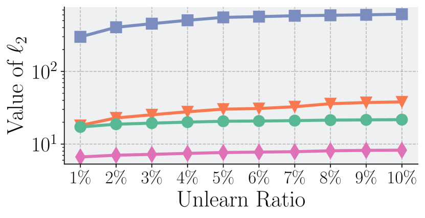
(a) Bounds vs. actual $\ell_{2}$ distance on Cora.

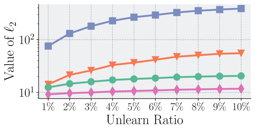
(b) Bounds vs. actual $\ell_{2}$ distance on CiteSeer.

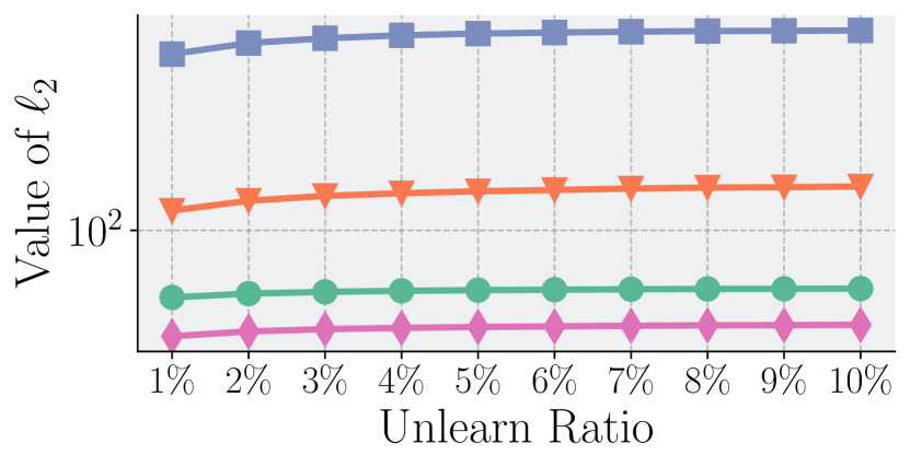
(c) Bounds vs. actual $\ell_{2}$ distance on PubMed.

Figure 5. Bounds and actual value of the $\ell_{2}$ distance between $\tilde{\bm{\theta}}^{*}$ and $\bar{\bm{\theta}}^{*}$, i.e., $\|\tilde{\bm{\theta}}^{*}-\bar{\bm{\theta}}^{*}\|_{2}$, over Cora, CiteSeer and PubMed datasets. CEU Worst, CEU Data Dependent, IDEA, and Actual represent the worst bound based on CEU, the data-dependent bound based on CEU, the bound based on IDEA, and the actual value of $\|\tilde{\bm{\theta}}^{*}-\bar{\bm{\theta}}^{*}\|_{2}$ derived from re-training, respectively.

Table 5. The running time (in seconds) of edge unlearning on Coauthor-CS dataset based on GCN. CGU is excluded from comparison since its backbone only support SGC. The running time of the proposed IDEA is marked in bold.

	0.1%	1%	5%	10%
Re-Training	170.0 $\pm$ 4.5	170.7 $\pm$ 5.6	169.8 $\pm$ 7.1	201.2 $\pm$ 14
Random	11.54 $\pm$ 0.8	11.09 $\pm$ 0.2	11.20 $\pm$ 0.2	11.07 $\pm$ 0.5
BEKM	9.66 $\pm$ 0.05	11.23 $\pm$ 0.3	10.88 $\pm$ 0.2	11.55 $\pm$ 0.3
BLPA	10.75 $\pm$ 0.1	10.71 $\pm$ 0.3	10.77 $\pm$ 0.2	10.94 $\pm$ 0.2
IDEA	2.823 $\pm$ 0.0	2.874 $\pm$ 0.1	2.851 $\pm$ 0.1	3.328 $\pm$ 0.1

Table 6. Node classification accuracy after edge unlearning. The results outside of brackets are accuracy values after unlearning with IDEA, while those inside brackets are given by re-training. The accuracy values of IDEA are marked in bold.

	0.1%	1%	5%	10%
Cora	81.18 $\pm$ 0.9 ( 84.50 $\pm$ 0.3 )	81.18 $\pm$ 1.4 ( 84.38 $\pm$ 0.3 )	79.34 $\pm$ 0.8 ( 82.41 $\pm$ 0.5 )	78.35 $\pm$ 1.0 ( 82.29 $\pm$ 0.3 )
CiteSeer	69.87 $\pm$ 1.3 ( 74.97 $\pm$ 0.3 )	69.87 $\pm$ 0.8 ( 75.38 $\pm$ 0.5 )	68.47 $\pm$ 0.8 ( 72.97 $\pm$ 0.7 )	67.27 $\pm$ 0.6 ( 73.57 $\pm$ 0.7 )
PubMed	81.02 $\pm$ 1.0 ( 84.99 $\pm$ 0.1 )	80.90 $\pm$ 0.9 ( 84.77 $\pm$ 0.0 )	79.63 $\pm$ 0.9 ( 83.82 $\pm$ 0.1 )	77.96 $\pm$ 0.8 ( 81.91 $\pm$ 0.1 )
CS	88.62 $\pm$ 5.4 ( 91.89 $\pm$ 1.6 )	92.42 $\pm$ 0.3 ( 92.73 $\pm$ 0.3 )	91.58 $\pm$ 0.3 ( 92.82 $\pm$ 0.1 )	90.91 $\pm$ 0.7 ( 91.84 $\pm$ 0.2 )
Physics	95.68 $\pm$ 0.4 ( 96.11 $\pm$ 0.2 )	95.64 $\pm$ 0.1 ( 96.03 $\pm$ 0.2 )	95.50 $\pm$ 0.3 ( 96.00 $\pm$ 0.2 )	95.19 $\pm$ 0.3 ( 95.86 $\pm$ 0.2 )

Appendix C Supplementary Experiments

C.1. Evaluation of Bound Tightness

In this subsection, we present additional experimental results regarding the bound tightness of the proposed model IDEA. Specifically, here we adopt SGC as our backbone GNN model, and we present the comparison between three bounds and actual value of the $\ell_{2}$ distance bound between $\tilde{\bm{\theta}}^{*}$ and $\bar{\bm{\theta}}^{*}$ in Figure 5.

We present an review of the introduction for the bounds and the $\ell_{2}$ distances below (as in Section 5.2). (1) CEU Worst Bound. We compute the theoretical worst bound derived based on CEU as a baseline of the $\ell_{2}$ distance bound between $\tilde{\bm{\theta}}^{*}$ and $\bar{\bm{\theta}}^{*}$. (2) CEU Data-Dependent Bound. We compute the data-dependent bound derived based on CEU as a baseline of the $\ell_{2}$ distance bound between $\tilde{\bm{\theta}}^{*}$ and $\bar{\bm{\theta}}^{*}$. Usually, data-dependent bound is tighter than the CEU Worst Bound. (3) IDEA Bound. We compute the bound given by Equation 6 as the IDEA bound for the $\ell_{2}$ distance bound between $\tilde{\bm{\theta}}^{*}$ and $\bar{\bm{\theta}}^{*}$. (4) Actual Values. We compare the bounds above with the actual values of the $\ell_{2}$ distance between $\tilde{\bm{\theta}}^{*}$ and $\bar{\bm{\theta}}^{*}$. In addition, we also follow the wide range of unlearning ratios as presented in Section 5.2.

Below we summarize the observations, which remains consistent with the observations presented in Section 5.2 and are also found on other GNNs and datasets. (1) From the perspective of the general tendency, we observe that when the value of unlearn ratio is increased (i.e., more edges are unlearned), it generally results in higher values for both the obtained bounds and the actual $\ell_{2}$ distance between $\tilde{\bm{\theta}}^{*}$ and $\bar{\bm{\theta}}^{*}$. This reveals that a higher unlearn ratio tends to make approximating $\tilde{\bm{\theta}}^{*}$ (using the calculated $\bar{\bm{\theta}}^{*}$) more difficult, which is also consistent with prior research (Wu et al., 2023a). (2) From the perspective of the bound tightness, the obtained results indicate that IDEA consistently provides tighter bounds than those produced by CEU across all scenarios, especially in cases with higher unlearn ratios. This suggests that the approximation of $\tilde{\bm{\theta}}^{*}$ offered by IDEA can capture the distance between $\tilde{\bm{\theta}}^{*}$ and $\bm{\theta}^{*}$ more accurately compared to CEU, especially for larger unlearn ratios.

C.2. Evaluation of Unlearning Efficiency

In this subsection, we present additional experimental results regarding the unlearning efficiency on different tasks. Specifically, we have shown efficiency comparison between IDEA and other baselines on node unlearning task in Section 5.3, and here we present additional results under edge unlearning task based on GCN, with all other settings being consistent with the experiments presented in Section 5.3. We show edge unlearning performance under a wide range of unlearning ratios (i.e., the ratio of edges to be unlearned to the total number of edges in the graph) from 0.1% to 10%. We present the experimental results in Table 5. We observe that the running time of the three variants of GraphEraser does not change as much as in Section 5.3 across the wide range of ratios. This is because GraphEraser perform partition over the input graph, which results in different shards. Each shard will contribute to the overall running time when the unlearn node/edge appear in such a shard. However, the number of edges is much more than the number of nodes. As a consequence, unlearn edges appears in most shards even if the unlearn ratio is as small as 0.1%. Hence most shards contribute to the running time in most cases, leading to a more stable running time across all ratios. Meanwhile, we also observe that IDEA not only achieves significantly less running time compared with the re-training approach, but also costs less running time compared with all other baselines. Such observation is consistent with the observation in Section 5.3, and can also be found on other datasets and GNNs. This indicates the superiority of IDEA in terms of the unlearning efficiency.

Table 7. AUC scores of attacks on Co-author CS based on GCN after node and edge unlearning, respectively. The results given by IDEA is marked in bold.

	Node Unlearning ($\downarrow$)	Edge Unlearning ($\downarrow$)
Random	51.51 $\pm$ 0.7	50.26 $\pm$ 0.4
BEKM	50.24 $\pm$ 0.8	50.26 $\pm$ 0.1
BLPA	51.42 $\pm$ 0.8	50.04 $\pm$ 0.2
IDEA	50.15 $\pm$ 0.8	50.02 $\pm$ 0.7

Table 8. Average loss values regarding the nodes with the unlearn attribute values being set to zero on CiteSeer. Lower values represents better unlearning performance, and the results given by IDEA are marked in bold.

	20% ($\downarrow$)	50% ($\downarrow$)	80% ($\downarrow$)
Random	1.44 $\pm$ 0.09	1.43 $\pm$ 0.08	1.48 $\pm$ 0.12
BEKM	1.44 $\pm$ 0.06	1.50 $\pm$ 0.04	1.51 $\pm$ 0.09
BLPA	1.40 $\pm$ 0.19	1.45 $\pm$ 0.27	1.50 $\pm$ 0.09
IDEA	1.25 $\pm$ 0.01	1.28 $\pm$ 0.01	1.33 $\pm$ 0.02

C.3. Evaluation of Model Utility

We now present additional results for the evaluation of model utility. We have shown the node classification accuracy comparison based on the SGC model in Section 5.4, and here we show the node classification accuracy comparison between IDEA and re-training based on the GCN model. We maintain all other settings to be consistent with those in Section 5.4. The model utility given by IDEA and re-training is compared across a wide range of unlearn ratio values (from 0.1% to 10% ). We observe that the unlearning given by IDEA only sacrifices limited utility compared with re-training, which remains consistent with the observation in Section 5.4, and such an observation can also be found on other datasets, unlearning tasks and GNNs. This indicates the satisfying usability of IDEA.

C.4. Evaluation of Unlearning Effectiveness

Finally, we present additional results for the evaluation of unlearning effectiveness. To evaluate the generalization capability of IDEA, here we utilize a different GNN model (compared with the results in Section 5.5), which is GCN, as the backbone. We adopt a consistent evaluation protocol as shown in Section 5.5, and we present the experimental results of node/edge unlearning and attribute unlearning in Table 7 and Table 8, respectively. We found that, first, in terms of node and edge unlearning tasks, we observe that the attacks on IDEA show the lowest attack successful AUC scores, which are marginally above 50% (almost equivalent to random guess). This indicates the effectiveness of IDEA in performing node and edge unlearning. Second, we observe that the average loss values given by IDEA are the lowest among all baselines. Since the loss values are collected from the nodes whose unlearn attribute values have already been set to zero, a lower loss value indicates better unlearning effectiveness. Therefore, the satisfying effectiveness of IDEA is further validated. Additionally, we note that these observations can also be found on other unlearning tasks, datasets, and GNNs, which indicates the satisfying unlearning effectiveness of IDEA.

References

- (1)
- Act (2000) Privacy Act. 2000. Personal Information Protection and Electronic Documents Act. Department of Justice, Canada. Full text available at http://laws. justice. gc. ca/en/P-8.6/text. html (2000).
- Bourtoule et al. (2021) Lucas Bourtoule, Varun Chandrasekaran, Christopher A Choquette-Choo, Hengrui Jia, Adelin Travers, Baiwu Zhang, David Lie, and Nicolas Papernot. 2021. Machine unlearning. In 2021 IEEE Symposium on Security and Privacy (SP). IEEE, 141–159.
- Cao and Yang (2015) Yinzhi Cao and Junfeng Yang. 2015. Towards making systems forget with machine unlearning. In 2015 IEEE symposium on security and privacy. IEEE, 463–480.
- Chen et al. (2022) Min Chen, Zhikun Zhang, Tianhao Wang, Michael Backes, Mathias Humbert, and Yang Zhang. 2022. Graph unlearning. In Proceedings of the 2022 ACM SIGSAC Conference on Computer and Communications Security. 499–513.
- Cheng et al. (2023) Jiali Cheng, George Dasoulas, Huan He, Chirag Agarwal, and Marinka Zitnik. 2023. GNNDelete: A General Strategy for Unlearning in Graph Neural Networks. arXiv preprint arXiv:2302.13406 (2023).
- Chien et al. (2022a) Eli Chien, Chao Pan, and Olgica Milenkovic. 2022a. Certified graph unlearning. arXiv preprint arXiv:2206.09140 (2022).
- Chien et al. (2022b) Eli Chien, Chao Pan, and Olgica Milenkovic. 2022b. Efficient model updates for approximate unlearning of graph-structured data. In The Eleventh International Conference on Learning Representations.
- Cook and Weisberg (1980) R Dennis Cook and Sanford Weisberg. 1980. Characterizations of an empirical influence function for detecting influential cases in regression. Technometrics 22, 4 (1980), 495–508.
- Dai et al. (2022) Enyan Dai, Tianxiang Zhao, Huaisheng Zhu, Junjie Xu, Zhimeng Guo, Hui Liu, Jiliang Tang, and Suhang Wang. 2022. A comprehensive survey on trustworthy graph neural networks: Privacy, robustness, fairness, and explainability. arXiv preprint arXiv:2204.08570 (2022).
- Do et al. (2019) Kien Do, Truyen Tran, and Svetha Venkatesh. 2019. Graph transformation policy network for chemical reaction prediction. In Proceedings of the 25th ACM SIGKDD international conference on knowledge discovery & data mining. 750–760.
- Dong et al. (2023a) Guimin Dong, Mingyue Tang, Zhiyuan Wang, Jiechao Gao, Sikun Guo, Lihua Cai, Robert Gutierrez, Bradford Campbel, Laura E Barnes, and Mehdi Boukhechba. 2023a. Graph neural networks in IoT: A survey. ACM Transactions on Sensor Networks 19, 2 (2023), 1–50.
- Dong et al. (2023b) Yushun Dong, Binchi Zhang, Yiling Yuan, Na Zou, Qi Wang, and Jundong Li. 2023b. Reliant: Fair knowledge distillation for graph neural networks. In Proceedings of the 2023 SIAM International Conference on Data Mining (SDM). SIAM, 154–162.
- Duan et al. (2022) Keyu Duan, Zirui Liu, Peihao Wang, Wenqing Zheng, Kaixiong Zhou, Tianlong Chen, Xia Hu, and Zhangyang Wang. 2022. A comprehensive study on large-scale graph training: Benchmarking and rethinking. Advances in Neural Information Processing Systems 35 (2022), 5376–5389.
- Dwork et al. (2014) Cynthia Dwork, Aaron Roth, et al. 2014. The algorithmic foundations of differential privacy. Foundations and Trends® in Theoretical Computer Science 9, 3–4 (2014), 211–407.
- Fan et al. (2019) Wenqi Fan, Yao Ma, Qing Li, Yuan He, Eric Zhao, Jiliang Tang, and Dawei Yin. 2019. Graph neural networks for social recommendation. In The world wide web conference. 417–426.
- Grimes et al. (2024) Keltin Grimes, Collin Abidi, Cole Frank, and Shannon Gallagher. 2024. Gone but Not Forgotten: Improved Benchmarks for Machine Unlearning. arXiv preprint arXiv:2405.19211 (2024).
- Guo et al. (2019) Chuan Guo, Tom Goldstein, Awni Hannun, and Laurens Van Der Maaten. 2019. Certified data removal from machine learning models. arXiv preprint arXiv:1911.03030 (2019).
- Guo et al. (2020) Chuan Guo, Tom Goldstein, Awni Y. Hannun, and Laurens van der Maaten. 2020. Certified Data Removal from Machine Learning Models. In Proceedings of the 37th International Conference on Machine Learning.
- Hamilton et al. (2017) Will Hamilton, Zhitao Ying, and Jure Leskovec. 2017. Inductive representation learning on large graphs. Advances in neural information processing systems 30 (2017).
- He et al. (2021) Xinlei He, Jinyuan Jia, Michael Backes, Neil Zhenqiang Gong, and Yang Zhang. 2021. Stealing links from graph neural networks. In 30th USENIX Security Symposium (USENIX Security 21). 2669–2686.
- Irwin et al. (2012) John J Irwin, Teague Sterling, Michael M Mysinger, Erin S Bolstad, and Ryan G Coleman. 2012. ZINC: a free tool to discover chemistry for biology. Journal of chemical information and modeling 52, 7 (2012), 1757–1768.
- Izzo et al. (2021) Zachary Izzo, Mary Anne Smart, Kamalika Chaudhuri, and James Zou. 2021. Approximate data deletion from machine learning models. In International Conference on Artificial Intelligence and Statistics. PMLR, 2008–2016.
- Jin et al. (2023) Yiqiao Jin, Yeon-Chang Lee, Kartik Sharma, Meng Ye, Karan Sikka, Ajay Divakaran, and Srijan Kumar. 2023. Predicting Information Pathways Across Online Communities. In KDD.
- Ju et al. (2024) Wei Ju, Siyu Yi, Yifan Wang, Zhiping Xiao, Zhengyang Mao, Hourun Li, Yiyang Gu, Yifang Qin, Nan Yin, Senzhang Wang, et al. 2024. A survey of graph neural networks in real world: Imbalance, noise, privacy and ood challenges. arXiv preprint arXiv:2403.04468 (2024).
- Kingma and Ba (2014) Diederik P Kingma and Jimmy Ba. 2014. Adam: A method for stochastic optimization. arXiv preprint arXiv:1412.6980 (2014).
- Kipf and Welling (2016) Thomas N Kipf and Max Welling. 2016. Semi-supervised classification with graph convolutional networks. arXiv preprint arXiv:1609.02907 (2016).
- Kipf and Welling (2017) Thomas N. Kipf and Max Welling. 2017. Semi-Supervised Classification with Graph Convolutional Networks. In 5th International Conference on Learning Representations.
- Koh and Liang (2017) Pang Wei Koh and Percy Liang. 2017. Understanding black-box predictions via influence functions. In International conference on machine learning. PMLR, 1885–1894.
- Kwak et al. (2017) Chanhee Kwak, Junyeong Lee, Kyuhong Park, and Heeseok Lee. 2017. Let machines unlearn–machine unlearning and the right to be forgotten. (2017).
- Liu et al. (2024a) Jiaqi Liu, Jian Lou, Zhan Qin, and Kui Ren. 2024a. Certified minimax unlearning with generalization rates and deletion capacity. Advances in Neural Information Processing Systems 36 (2024).
- Liu et al. (2024b) Ziyao Liu, Huanyi Ye, Chen Chen, and Kwok-Yan Lam. 2024b. Threats, attacks, and defenses in machine unlearning: A survey. arXiv preprint arXiv:2403.13682 (2024).
- Ma et al. (2022) Jing Ma, Yushun Dong, Zheng Huang, Daniel Mietchen, and Jundong Li. 2022. Assessing the causal impact of COVID-19 related policies on outbreak dynamics: A case study in the US. In Proceedings of the ACM Web Conference 2022. 2678–2686.
- Mahadevan and Mathioudakis (2021) Ananth Mahadevan and Michael Mathioudakis. 2021. Certifiable machine unlearning for linear models. arXiv preprint arXiv:2106.15093 (2021).
- Neo et al. (2024) Neng Kai Nigel Neo, Yeon-Chang Lee, Yiqiao Jin, Sang-Wook Kim, and Srijan Kumar. 2024. Towards Fair Graph Anomaly Detection: Problem, New Datasets, and Evaluation. arXiv:2402.15988 (2024).
- Nguyen et al. (2022) Thanh Tam Nguyen, Thanh Trung Huynh, Phi Le Nguyen, Alan Wee-Chung Liew, Hongzhi Yin, and Quoc Viet Hung Nguyen. 2022. A survey of machine unlearning. arXiv preprint arXiv:2209.02299 (2022).
- Olatunji et al. (2021) Iyiola E Olatunji, Wolfgang Nejdl, and Megha Khosla. 2021. Membership inference attack on graph neural networks. In Third IEEE International Conference on Trust, Privacy and Security in Intelligent Systems and Applications. IEEE, 11–20.
- Pan et al. (2023) Chao Pan, Eli Chien, and Olgica Milenkovic. 2023. Unlearning graph classifiers with limited data resources. In Proceedings of the ACM Web Conference 2023. 716–726.
- Pardau (2018) Stuart L Pardau. 2018. The california consumer privacy act: Towards a european-style privacy regime in the united states. J. Tech. L. & Pol’y 23 (2018), 68.
- Paszke et al. (2017) Adam Paszke, Sam Gross, Soumith Chintala, Gregory Chanan, Edward Yang, Zachary DeVito, Zeming Lin, Alban Desmaison, Luca Antiga, and Adam Lerer. 2017. Automatic differentiation in pytorch. (2017).
- Qiu et al. (2022) Yeqing Qiu, Chenyu Huang, Jianzong Wang, Zhangcheng Huang, and Jing Xiao. 2022. A privacy-preserving subgraph-level federated graph neural network via differential privacy. In International Conference on Knowledge Science, Engineering and Management. Springer, 165–177.
- Qu et al. (2023) Youyang Qu, Xin Yuan, Ming Ding, Wei Ni, Thierry Rakotoarivelo, and David Smith. 2023. Learn to unlearn: A survey on machine unlearning. arXiv preprint arXiv:2305.07512 (2023).
- Regulation (2018) General Data Protection Regulation. 2018. General data protection regulation (GDPR). Intersoft Consulting, Accessed in October 24, 1 (2018).
- Said et al. (2023) Anwar Said, Tyler Derr, Mudassir Shabbir, Waseem Abbas, and Xenofon Koutsoukos. 2023. A Survey of Graph Unlearning. preprint arXiv:2310.02164 (2023).
- Sajadmanesh (2023) Sina Sajadmanesh. 2023. Privacy-Preserving Machine Learning on Graphs. Technical Report. EPFL.
- Schelter et al. (2023) Sebastian Schelter, Mozhdeh Ariannezhad, and Maarten de Rijke. 2023. Forget me now: Fast and exact unlearning in neighborhood-based recommendation. In Proceedings of the 46th International ACM SIGIR Conference on Research and Development in Information Retrieval. 2011–2015.
- Sekhari et al. (2021) Ayush Sekhari, Jayadev Acharya, Gautam Kamath, and Ananda Theertha Suresh. 2021. Remember what you want to forget: Algorithms for machine unlearning. Advances in Neural Information Processing Systems 34 (2021), 18075–18086.
- Shan et al. (2021) Chuanqiang Shan, Huiyun Jiao, and Jie Fu. 2021. Towards representation identical privacy-preserving graph neural network via split learning. arXiv preprint arXiv:2107.05917 (2021).
- Shchur et al. (2018) Oleksandr Shchur, Maximilian Mumme, Aleksandar Bojchevski, and Stephan Günnemann. 2018. Pitfalls of graph neural network evaluation. arXiv preprint arXiv:1811.05868 (2018).
- Shi et al. (2023) Yucheng Shi, Yushun Dong, Qiaoyu Tan, Jundong Li, and Ninghao Liu. 2023. Gigamae: Generalizable graph masked autoencoder via collaborative latent space reconstruction. In Proceedings of the 32nd ACM International Conference on Information and Knowledge Management. 2259–2269.
- Thudi et al. (2022) Anvith Thudi, Gabriel Deza, Varun Chandrasekaran, and Nicolas Papernot. 2022. Unrolling sgd: Understanding factors influencing machine unlearning. In 2022 IEEE 7th European Symposium on Security and Privacy (EuroS&P). IEEE, 303–319.
- Veličković et al. (2017) Petar Veličković, Guillem Cucurull, Arantxa Casanova, Adriana Romero, Pietro Lio, and Yoshua Bengio. 2017. Graph attention networks. arXiv preprint arXiv:1710.10903 (2017).
- Wang et al. (2019) Daixin Wang, Jianbin Lin, Peng Cui, Quanhui Jia, Zhen Wang, Yanming Fang, Quan Yu, Jun Zhou, Shuang Yang, and Yuan Qi. 2019. A semi-supervised graph attentive network for financial fraud detection. In 2019 IEEE International Conference on Data Mining (ICDM). IEEE, 598–607.
- Wang et al. (2024) Weiqi Wang, Zhiyi Tian, and Shui Yu. 2024. Machine Unlearning: A Comprehensive Survey. arXiv preprint arXiv:2405.07406 (2024).
- Wang et al. (2023) Xuemin Wang, Tianlong Gu, Xuguang Bao, and Liang Chang. 2023. Fair and Privacy-Preserving Graph Neural Network. In International Conference on Database Systems for Advanced Applications. Springer, 731–735.
- Wang et al. (2022) Yu Wang, Yuying Zhao, Yushun Dong, Huiyuan Chen, Jundong Li, and Tyler Derr. 2022. Improving fairness in graph neural networks via mitigating sensitive attribute leakage. In Proceedings of the 28th ACM SIGKDD conference on knowledge discovery and data mining. 1938–1948.
- Warnecke et al. (2021) Alexander Warnecke, Lukas Pirch, Christian Wressnegger, and Konrad Rieck. 2021. Machine unlearning of features and labels. preprint arXiv:2108.11577 (2021).
- Wu et al. (2021) Bang Wu, Xiangwen Yang, Shirui Pan, and Xingliang Yuan. 2021. Adapting membership inference attacks to GNN for graph classification: Approaches and implications. In IEEE International Conference on Data Mining (ICDM). IEEE.
- Wu et al. (2019a) Felix Wu, Amauri Souza, Tianyi Zhang, Christopher Fifty, Tao Yu, and Kilian Weinberger. 2019a. Simplifying graph convolutional networks. In International conference on machine learning. PMLR, 6861–6871.
- Wu et al. (2023b) Jiancan Wu, Yi Yang, Yuchun Qian, Yongduo Sui, Xiang Wang, and Xiangnan He. 2023b. GIF: A General Graph Unlearning Strategy via Influence Function. In Proceedings of the ACM Web Conference 2023. 651–661.
- Wu et al. (2023a) Kun Wu, Jie Shen, Yue Ning, Ting Wang, and Wendy Hui Wang. 2023a. Certified edge unlearning for graph neural networks. In Proceedings of the 29th ACM SIGKDD Conference on Knowledge Discovery and Data Mining. 2606–2617.
- Wu et al. (2022) Lingfei Wu, Peng Cui, Jian Pei, Liang Zhao, and Xiaojie Guo. 2022. Graph neural networks: foundation, frontiers and applications. In Proceedings of the 28th ACM SIGKDD Conference on Knowledge Discovery and Data Mining. 4840–4841.
- Wu et al. (2019b) Shu Wu, Yuyuan Tang, Yanqiao Zhu, Liang Wang, Xing Xie, and Tieniu Tan. 2019b. Session-based recommendation with graph neural networks. In Proceedings of the AAAI conference on artificial intelligence, Vol. 33. 346–353.
- Wu et al. (2020) Zonghan Wu, Shirui Pan, Fengwen Chen, Guodong Long, Chengqi Zhang, and S Yu Philip. 2020. A comprehensive survey on graph neural networks. IEEE transactions on neural networks and learning systems 32, 1 (2020), 4–24.
- Xu et al. (2023b) Heng Xu, Tianqing Zhu, Lefeng Zhang, Wanlei Zhou, and Philip S Yu. 2023b. Machine unlearning: A survey. Comput. Surveys 56, 1 (2023), 1–36.
- Xu et al. (2024) Jie Xu, Zihan Wu, Cong Wang, and Xiaohua Jia. 2024. Machine unlearning: Solutions and challenges. IEEE Transactions on Emerging Topics in Computational Intelligence (2024).
- Xu et al. (2018) Keyulu Xu, Weihua Hu, Jure Leskovec, and Stefanie Jegelka. 2018. How powerful are graph neural networks? arXiv preprint arXiv:1810.00826 (2018).
- Xu et al. (2019) Keyulu Xu, Weihua Hu, Jure Leskovec, and Stefanie Jegelka. 2019. How Powerful are Graph Neural Networks?. In 7th International Conference on Learning Representations.
- Xu et al. (2023a) Wanghan Xu, Bin Shi, Jiqiang Zhang, Zhiyuan Feng, Tianze Pan, and Bo Dong. 2023a. MDP: Privacy-Preserving GNN Based on Matrix Decomposition and Differential Privacy. In 2023 IEEE International Conference on Joint Cloud Computing (JCC). IEEE, 38–45.
- Yan et al. (2022) Haonan Yan, Xiaoguang Li, Ziyao Guo, Hui Li, Fenghua Li, and Xiaodong Lin. 2022. ARCANE: An Efficient Architecture for Exact Machine Unlearning.. In IJCAI, Vol. 6. 19.
- Zhang et al. (2023a) Binchi Zhang, Yushun Dong, Chen Chen, Yada Zhu, Minnan Luo, and Jundong Li. 2023a. Adversarial Attacks on Fairness of Graph Neural Networks. arXiv preprint arXiv:2310.13822 (2023).
- Zhang et al. (2023b) Haibo Zhang, Toru Nakamura, Takamasa Isohara, and Kouichi Sakurai. 2023b. A review on machine unlearning. SN Computer Science 4, 4 (2023), 337.
- Zhang et al. (2021) Xiao-Meng Zhang, Li Liang, Lin Liu, and Ming-Jing Tang. 2021. Graph neural networks and their current applications in bioinformatics. Frontiers in genetics 12 (2021), 690049.
- Zhang et al. (2023c) Yi Zhang, Yuying Zhao, Zhaoqing Li, Xueqi Cheng, Yu Wang, Olivera Kotevska, Philip S Yu, and Tyler Derr. 2023c. A Survey on Privacy in Graph Neural Networks: Attacks, Preservation, and Applications. arXiv preprint arXiv:2308.16375 (2023).
- Zhang et al. (2022) Zijie Zhang, Yang Zhou, Xin Zhao, Tianshi Che, and Lingjuan Lyu. 2022. Prompt certified machine unlearning with randomized gradient smoothing and quantization. Advances in Neural Information Processing Systems 35 (2022), 13433–13455.
- Zheng et al. (2020) Chuanpan Zheng, Xiaoliang Fan, Cheng Wang, and Jianzhong Qi. 2020. Gman: A graph multi-attention network for traffic prediction. In Proceedings of the AAAI conference on artificial intelligence, Vol. 34. 1234–1241.
- Zheng et al. (2023) Wenyue Zheng, Ximeng Liu, Yuyang Wang, and Xuanwei Lin. 2023. Graph Unlearning Using Knowledge Distillation. In International Conference on Information and Communications Security. Springer, 485–501.
- Zhou et al. (2020) Jie Zhou, Ganqu Cui, Shengding Hu, Zhengyan Zhang, Cheng Yang, Zhiyuan Liu, Lifeng Wang, Changcheng Li, and Maosong Sun. 2020. Graph neural networks: A review of methods and applications. AI open 1 (2020), 57–81.
- Zitnik et al. (2018) Marinka Zitnik, Monica Agrawal, and Jure Leskovec. 2018. Modeling polypharmacy side effects with graph convolutional networks. Bioinformatics 34, 13 (2018), i457–i466.