Penalized Principal Component Analysis for Large-dimension Factor Model with Group Pursuit

Abstract

This paper investigates the intrinsic group structures within the framework of large-dimensional approximate factor models, which portrays homogeneous effects of the common factors on the individuals that fall into the same group. To this end, we propose a fusion Penalized Principal Component Analysis (PPCA) method and derive a closed-form solution for the $\ell_{2}$-norm optimization problem. We also show the asymptotic properties of our proposed PPCA estimates. With the PPCA estimates as an initialization, we identify the unknown group structure by a combination of the agglomerative hierarchical clustering algorithm and an information criterion. Then the factor loadings and factor scores are re-estimated conditional on the identified latent groups. Under some regularity conditions, we establish the consistency of the membership estimators as well as that of the group number estimator derived from the information criterion. Theoretically, we show that the post-clustering estimators for the factor loadings and factor scores with group pursuit achieve efficiency gains compared to the estimators by conventional PCA method. Thorough numerical studies validate the established theory and a real financial example illustrates the practical usefulness of the proposed method.

1 Introduction

As a powerful technique for data simplification and dimension reduction, factor models are widely used to extract representative features and explain the generative process of massive variables. They have been applied in various fields such as financial engineering, economic analysis and biological technology, including studying the expected returns (Ross, 2013, 1977; Fama and French, 1992, 1993), risks of portfolios (Fan et al., 2015) and gene expression data (Mayrink and Lucas, 2013). Factor models have also been combined with many modern statistical leaning methods to improve predictive power, such as factor profiled sure independence screening in Wang (2012), the estimation of large covariance matrices in Fan et al. (2018) and factor-adjusted multiple testing in Fan et al. (2019).

Thus far, the most effective tools for analyzing and predicting large-dimensional time series are the large-dimensional (approximate) factor models, which allow the idiosyncratic errors to be cross-sectionally correlated (Chamberlain and Rothschild, 1982). The estimation and inference for factor models are crucial in economic studies, particularly in areas such as asset pricing and return forecasting. With the increase of data dimension in these areas, how to accurately estimate and infer the unknown factor scores and loadings becomes more and more challenging and attracts growing attention of econometricians. Principal component analysis (PCA) method and Maximum Likelihood Estimation (MLE) method are two common methods for inferring factor models, whose asymptotic properties have been fully explored in the literature, see for example, Bai and Ng (2002), Bai (2003), Forni et al. (2005), Bai and Li (2012), Bai and Li (2016), Chen et al. (2021a), Wang (2022), Ma and Tu (2023). In particular, the PCA method, known for its simplicity and effectiveness, is closely connected with the factor model and has long been a hot research topic in the econometric community. An increasing number of work focus on more flexible factor models, for instance, factor models with structural breaks (Bates et al., 2013; Baltagi et al., 2017); constrained factor model (Tsai and Tsay, 2010); factor model with latent group structures (Tu and Wang, 2023; He et al., 2024b); robust factor analysis (Yu et al., 2019; Chen et al., 2021b; He et al., 2022); matrix/tesnor factor models (Han et al., 2020, 2022; Chen et al., 2022; Yu et al., 2022; He et al., 2023a, b, 2024a; Barigozzi et al., 2024).

In the era of “big data”, the cross-sectional dimension in the approximate factor models typically grows extremely large, thus the number of unknown parameters increases dramatically, which causes great challenges for accurate estimation. To alleviate this issue, Tsai and Tsay (2010) proposed a constrained factor model to study the monthly U.S. excess stock returns where the stocks within the same sector of industry are assumed to share the same loadings on risk factors. In addition, Xiang et al. (2023) divided the cities into four groups and assume the market and government factors have the same impact on house price growth within each group. Both the studies have assumed the group information is pre-specified, which lack support of economic theory. Consequently, the derived results can be misleading when the group membership is misspecified. As an alternative, Tu and Wang (2023) assume the loading vectors in the factor model have a latent group structure, portraying the homogeneous effects of the common factors on the individuals falling into the same group. He et al. (2024b) also propose robust estimators of the factors and factor loadings in the presence of both group structure and heavy-tailedness.

This paper is inspired by a growing literature on homogeneity in panel data, such as Wang et al. (2018), Vogt and Linton (2017), Ma and Huang (2017),Chen (2019), Ma et al. (2020), Chen et al. (2021a), Guo and Li (2022), Wei et al. (2023), Tu and Wang (2023) and Wang and Zhu (2024). Without resorting to any prior information, we develop a completely data-driven unsupervised grouping criterion for the cross-sectional units under the framework of approximate factor model. Our proposed method mainly include the following two steps. In the first step, we propose a fusion Penalized Principal Component Analysis (PPCA) method to derive an initial estimator with group structure. Interestingly, a closed-form solution for the penalized optimization problem is derived in this paper, which is computationally as efficient as the traditional PCA method. In the second step, we apply the classical hierarchical clustering (AHC) method to the $\ell_{1}$-distance between the estimated loading vectors by PPCA derived from the first step. We summarize the major contributions of this paper as follows. Firstly, we propose a fusion Penalised PCA (PPCA) method for estimating the factor scores and factor loadings. A novel $\ell_{2}$ type fusion penalty is exerted on the pairwise loading vectors to encourage similarity of loadings for individuals within the same group, which results in a closed-form solution. We then compare it with the traditional PCA method and derive the consistency and asymptotic normality of the PPCA estimators. Secondly, we introduce a clustering procedure for determining the group membership of each cross-sectional unit and an information criteria for selecting the number of groups. We investigate the asymptotic properties of the clustering procedure, which demonstrates that the proposed method can accurately identify the group memberships and estimate the group number with probability approaching to 1. In addition, we have also established the asymptotic properties of the post-grouping estimators of the factor loadings. Thorough simulation experiments verify the well finite sample performance of the proposed method in terms of both identifying group memberships and selecting group number. We use our proposed approach to analyze a portfolio returns dataset, in which we discover intriguing patterns of clustering that contribute to a substantial enhancement in predictive accuracy.

The rest of the paper is structured as follows. Section 2 introduces the approximate factor model with group homogeneity, and we propose the novel PPCA method to estimate the factor scores and factor loadings. Meanwhile this section also introduces the clustering method and an information criterion for identifying the latent group structure and estimating the unknown group number, respectively. Section 3 establishes the asymptotic properties of the proposed PPCA estimators and the subsequent estimators of the clustering procedure. Section 4 displays the finite sample performance of the proposed method by simulation studies, and Section 5 illustrates its practical merits with an U.S. portfolio return dataset. Section 6 concludes the paper and discusses possible future research directions. All the technical proofs of the theorems and additional empirical results are relegated to the supplementary material.

To end this section, we introduce some notations used throughout this paper. Denote $\bm{0}_{p}$ as the $p$-dimensional vector with all elements zero. For a vector $\bm{a}$, we denote $||\bm{a}||_{q}$ as its $\ell_{q}$ norm. Denote $\mathbf{I}_{p}$ as the $p$-dimensional identity matrix. For a matrix $\mathbf{A}$, $\text{Tr}(\mathbf{A})$ denotes the trace of $\mathbf{A}$. We denote $\lambda_{j}(\mathbf{A})$ as the $j$-th largest eigenvalue of a symmetric matrix $\mathbf{A}$ while $\lambda_{\max}(\mathbf{A})$ and $\lambda_{\min}(\mathbf{A})$ correspond to the maximum and minimum eigenvalue, respectively. We define $||\mathbf{A}||_{F}=\text{Tr}^{1/2}(\mathbf{A}^{\top}\mathbf{A})$, $||\mathbf{A}||=\lambda^{1/2}_{\max}(\mathbf{A}^{\top}\mathbf{A})$ as the Frobenius norm and the spectral norm of $\mathbf{A}$ respectively. $X_{n}\lesssim Y_{n}$ means there exists a constant $c>0$ such that $X_{n}\leq cY_{n}$ for sufficiently large $n$, while $X_{n}\gtrsim Y_{n}$ means there exists a constant $c>0$ such that $X_{n}>cY_{n}$ for sufficiently large $n$, and $X_{n}\asymp Y_{n}$ means both $X_{n}\leq cY_{n}$ and $X_{n}\gtrsim Y_{n}$ hold. The cardinality of a set $\mathcal{G}$ is denoted as $|\mathcal{G}|$. The constants $c$ and $M$ in different lines can be not identical.

2 Methodology

In this section, we formally introduce our method which includes two main steps. Firstly, we introduce a pairwise fusion penalty to encourage group pursuit for the factor loadings, thereby putting forward the Penalized PCA method to enhance estimation accuracy for the factor structure. To identify group memberships, we perform the AHC algorithm to cluster the individuals into groups, then further deriving refined post-grouping estimators of the factor loadings.

2.1 Preliminary

Consider the static approximate factor model originated from Chamberlain and Rothschild (1982) for a large panels $\{x_{ti}\}_{i\leq N,t\leq T}$,

$$x_{ti}=\sum_{l=1}^{r}b_{il}f_{tl}+e_{ti},\quad\text{for}\quad t=1,\ldots,T,i=1,\ldots,N.$$ (2.1)

where $b_{il}$ are the factor loadings, $f_{tl}$ are the random factor scores, $e_{ti}$ are the idiosyncratic errors which can be cross-sectionally correlated, $r$ is the number of common factors. In model (2.1), only $x_{ti}$ can be observed, while $r$, $b_{il}$, $f_{tl}$ and $e_{ti}$ are all unobserved. In this paper, one of our research interest is to refine the estimates of the unknown factor loadings and factor scores by traditional PCA given the prior knowledge of the existence of latent groups of individuals.

The vector and matrix form of model (2.1) are as follows

$$\mathbf{x}_{t}=\mathbf{B}\bm{f}_{t}+\mathbf{e}_{t},\quad\mathbf{X}=\mathbf{F}\mathbf{B}^{\top}+\mathbf{E}$$ (2.2)

where $\mathbf{x}_{t}^{\top}=(x_{t1},\ldots,x_{tN})$, $\mathbf{B}=(\bm{b}_{1},...,\bm{b}_{N})^{\top}=(b_{il})_{N\times r}$, $\bm{f}_{t}^{\top}=(f_{t1},\ldots,f_{tr})$, $\mathbf{e}_{t}^{\top}=(e_{t1},\ldots,e_{tN})$, $\mathbf{X}=(x_{ti})_{T\times N}$, $\mathbf{F}=(f_{tl})_{T\times r}$ and $\mathbf{E}=(e_{ti})_{T\times N}$. From model (2.2), we can see there exists an identifiable issue among the common factor scores and the factor loadings. In this paper, we assume $\mathbf{F}^{\top}\mathbf{F}/T=\mathbf{I}_{r}$ almost surely as $T\rightarrow\infty$ to ensure identifiability up to orthogonal transformations, see for example Bai and Li (2012) and Bai (2003) for more detailed discussions on the identifiability issue. Model (2.1) typically can be estimated by Principle Component Analysis(PCA) and Maximum Likelihood Estimation(MLE), see for example Bai (2003) and Bai and Li (2012). In this paper, we primarily focus on the PCA method. A conventional PCA solution to Model (2.1) in Bai (2003) is to minimize

$$Q_{1}(\mathbf{B},\mathbf{F})=(NT)^{-1}||\mathbf{X}-\mathbf{F}\mathbf{B}^{\top}||_{F}^{2},\quad\text{s.t.}\quad\mathbf{F}^{\top}\mathbf{F}/T=\mathbf{I}_{r}.$$

The factor number $r$ can be estimated by the Information Criterion (IC) by Bai and Ng (2002) or other criteria such as Eigenvalue-Ratio (ER) by Ahn and Horenstein (2013). Let the columns of $\widehat{\mathbf{F}}$ be $\sqrt{T}$ times the leading $r$ eigenvectors of $\mathbf{X}\mathbf{X}^{\top}$, then the solution to minimizing the loss function $Q_{1}(\mathbf{B},\mathbf{F})$ is $\widehat{\mathbf{B}}=T^{-1}\mathbf{X}^{\top}\widehat{\mathbf{F}}.$ Therefore, the estimators of the common components are naturally $\widehat{c}_{ti}=\sum_{l=1}^{r}\widehat{b}_{il}\widehat{f}_{tl}$. The theoretical properties of $\widehat{b}_{il}$, $\widehat{f}_{tl}$, and $\widehat{c}_{ti}$ are given in Bai (2003) for the large-dimensional case where $N,T\rightarrow\infty$.

When it comes to the convergence rates of the loadings estimators, although the assumption that the dimension of the loading vector $\bm{b}_{i}$ is often relatively small which significantly decreases the number of unknown parameters, however due to the individual specific nature of the factor loadings, the total number of the loading vectors to be estimated is equal to the number of the cross-sectional units $N$. This still would make the convergence rate of the loadings estimators relatively slow, as given by Bai (2003). To avoid fitting too many parameters, it’s typically assumed that there exist certain types of structural sparsity, which would further reduce the dimension of the parameters of interest and is plausible in many real scenarios such as analyzing repetitive psychology tests scores.

In this paper, we consider a similar setting as in Tu and Wang (2023) and He et al. (2024b) and assume the approximate factor model has a latent group homogeneity structure, where factor loadings are the same across units that fall into the same group. Assume there is a partition of index set $\{1,\ldots,N\}$, denoted by $\{\mathcal{G}_{1},\ldots,\mathcal{G}_{K_{0}}\}$ such that

$$\bm{b}_{i}=\sum_{k=1}^{K_{0}}\bm{b}_{\mathcal{G},k}\cdot\mathbbm{1}\{i\in\mathcal{G}_{k}\}\quad\text{and}\quad\mathcal{G}_{k}\cap\mathcal{G}_{j}=\emptyset\quad\text{for}\quad k\neq j,$$ (2.3)

where $K_{0}$ is the true number of latent groups which is assumed to be finite but unknown, $\bm{b}_{\mathcal{G},k}$ is the common value of the loading vectors whose index is in $\mathcal{G}_{k}$, $\mathbbm{1}\{\cdot\}$ denotes the indicator function and $\varnothing$ denotes the empty set. From the group homogeneity condition (2.3), it’s easy to see that the individuals in the same group share the common loading vectors so as to induce the dimension of the loading vectors from $N$ to $K_{0}$. The group number $K_{0}$ and the true group $\{\mathcal{G}_{1},\ldots,\mathcal{G}_{K_{0}}\}$ are all unknown, and in the following section we propose a novel PPCA method to estimate the factor loadings and then apply an AHC procedure to the PPCA estimators to derive the estimators of group memberships.

2.2 PPCA method for estimating factor loadings and scores

In Model (2.1), only $x_{it}$ can be observed and our goal in this section is to give a more accurate estimate of the factor scores and factor loadings with prior knowledge of latent group structure. We exploit the pairwise fusion penalty in the literature and propose a Penalized PCA approach with a given $r$ to encourage the sparsity of $(\bm{b}_{i}-\bm{b}_{j})$, namely,

$$\left(\widehat{\mathbf{B}},\widehat{\mathbf{F}}\right)=\mathop{\mathrm{argmin}}_{\mathbf{B},\mathbf{F}}\frac{1}{TN}||\mathbf{X}-\mathbf{F}\mathbf{B}^{\top}||_{F}^{2}+\widetilde{\lambda}\sum_{i<j}||\bm{b}_{i}-\bm{b}_{j}||^{2},\quad\text{s.t.}\quad\mathbf{F}^{\top}\mathbf{F}/T=\mathbf{I}_{r},$$ (2.4)

where $\widetilde{\lambda}>0$ is a tuning parameter. Clearly, a sufficiently small $\widetilde{\lambda}$ implies that there may not exist group structures and our estimator degenerates into the traditional PCA method. On the contrary, a sufficiently large $\widetilde{\lambda}$ would force all individuals share the same factor loadings. Therefore, a moderate $\widetilde{\lambda}$ would lead to heterogeneous group structures of the factor loadings. The tuning parameter $\widetilde{\lambda}$ typically can be determined by cross validation.

At a first glance, the optimization problem seems to be difficult as there is $N(N-1)$ penalties in (2.4). Interestingly, we derive a closed-form solution to the optimization problem. For better illustration, we first let

$$\mathcal{L}(\mathbf{B},\mathbf{F})=\frac{1}{TN}||\mathbf{X}-\mathbf{F}\mathbf{B}^{\top}||_{F}^{2}+\widetilde{\lambda}\sum_{i<j}||\bm{b}_{i}-\bm{b}_{j}||^{2},\quad\text{s.t.}\quad\mathbf{F}^{\top}\mathbf{F}/T=\mathbf{I}_{r}.$$ (2.5)

By the Laplacian matrix, define $\bm{\Pi}=N\mathbf{I}_{N}-\mathbf{A}$ where $\mathbf{A}$ is a $N\times N$ all one matrix, i.e., $\mathbf{A}=(1)_{N\times{N}}$. Meanwhile, we define the normalized form of $\bm{\Pi}$ as $\bm{\Pi}_{N}=\frac{1}{N}\bm{\Pi}$, then we would have

$$\sum_{i<j}||\bm{b}_{i}-\bm{b}_{j}||^{2}=N\text{Tr}(\mathbf{B}^{\top}\bm{\Pi}_{N}\mathbf{B}).$$

Denote $\lambda=N^{2}\widetilde{\lambda}$, thus we have

$$\mathcal{L}(\mathbf{B},\mathbf{F}) =\frac{1}{TN}||\mathbf{X}-\mathbf{F}\mathbf{B}^{\top}||_{F}^{2}+\frac{\lambda}{N}\text{Tr}(\mathbf{B}^{\top}\bm{\Pi}_{N}\mathbf{B})$$ (2.6)

$$=\frac{1}{NT}\text{Tr}(\mathbf{X}^{\top}\mathbf{X})-\frac{1}{NT^{2}}\text{Tr}(\mathbf{X}^{\top}\mathbf{F}\mathbf{F}^{\top}\mathbf{X})+\frac{1}{N}||T^{-1}\mathbf{X}^{\top}\mathbf{F}-\mathbf{B}||_{F}^{2}+\frac{\lambda}{N}\text{Tr}(\mathbf{B}^{\top}\bm{\Pi}_{N}\mathbf{B}).$$

We first assume $\lambda$ and $\widehat{\mathbf{F}}$ are given while $\widehat{\mathbf{F}}^{\top}\widehat{\mathbf{F}}/T=\mathbf{I}_{r}$. Therefore, the solution with respect to the factor loadings would be

$$\widehat{\mathbf{B}}=\frac{1}{T}\mathbf{D}^{-1}\mathbf{X}^{\top}\widehat{\mathbf{F}},$$ (2.7)

where $\mathbf{D}=\mathbf{I}+\lambda\bm{\Pi}_{N}$ and it depends on the tuning parameter $\lambda$ and $N$. Then take $\widehat{\mathbf{B}}=\mathbf{D}^{-1}\mathbf{X}^{\top}\widehat{\mathbf{F}}/T$ back to $\mathcal{L}(\mathbf{B},\mathbf{F})$, we have

$$\mathcal{L}(\widehat{\mathbf{B}},\mathbf{F})=\frac{1}{NT}\text{Tr}(\mathbf{X}^{\top}\mathbf{X})-\frac{1}{NT^{2}}\text{Tr}(\mathbf{F}^{\top}\mathbf{X}\mathbf{D}^{-1}\mathbf{X}^{\top}\mathbf{F}).$$

Thus the solution with respect to the factor scores ${\mathbf{F}}$ can be taken as $\sqrt{T}$ times the leading $r$ eigenvectors of $\mathbf{X}\mathbf{D}^{-1}\mathbf{X}^{\top}$. For the selection of tuning parameter $\lambda$, in this subsection, we use a Cross-Validation(CV) to find the $\lambda$, which minimizes $||\mathbf{X}-\widehat{\mathbf{F}}\widehat{\mathbf{B}}^{\top}||_{F}^{2}$ at each validation step.

Intuitively, it is straightforward to replace the $\ell_{2}$ norm penalty by a general $\ell_{q}$ norm, i.e., $||\bm{b}_{i}-\bm{b}_{j}||_{q}$, which would also be appropriate for group pursuits. However, we prefer the proposed $\ell_{2}$ norm penalty as in this case we acquire a closed-form solution, i.e, we just need to perform eigen-decomposition of $\mathbf{X}\mathbf{D}^{-1}\mathbf{X}^{\top}$, which is computationally as efficient as traditional PCA and significantly alleviates computational burdens compared with other $\ell_{q}$ norms. Indeed, $\ell_{2}$ relaxation has been widely explored in the econometrics literature,for example, Shi et al. (2022) adopt $\ell_{2}$ relaxation to tackle forecast combination with many forecasts or minimum variance portfolio selection with many assets.

One disadvantage of the squared $\ell_{2}$-norm penalty lies in that the estimator $\widehat{\mathbf{B}}$ in equation (2.7) would not show strict group structure, that is, for some index pairs $(i,j)$, $\widehat{b}_{i}-\widehat{b}_{j}$ can be sufficiently small but not exactly zero. Therefore, it is necessary to further resort to some clustering algorithms to identify the latent groups. However, it’s worth pointing out that our proposed Penalized PCA method would deliver a more efficient estimator in certain cases compared with the traditional PCA method, which benefits the downstream clustering procedure.

2.3 Homogeneity pursuit

As long as we obtain the PPCA estimators in the first step, various clustering algorithms can be used to recover the latent group memberships based on the PPCA estimators, such as the well known $K$-means or Agglomerative hierarchical clustering (AHC). In this paper, we also adopt the classical AHC algorithm to identify the latent homogeneity structure in the loading vectors with a given factor number $r$, for ease of presentation and comparison with Tu and Wang (2023) and He et al. (2024b). In detail, we first define the distance measure between $\bm{b}_{i}$ and $\bm{b}_{j}$ as:

$$\Delta_{ij}=\frac{1}{r}||\mathbf{H}^{\top}(\bm{b}_{i}-\bm{b}_{j})||_{1},$$ (2.8)

where $\mathbf{H}$ is an $r\times r$ rotation matrix. From (2.8), we can easily see that if $i,j\in\mathcal{G}_{k}$, $\Delta_{ij}=0$ while $\Delta_{ij}\neq 0$ if $i\in\mathcal{G}_{k_{1}}$ and $j\in\mathcal{G}_{k_{2}}$, whenever $k_{1}\neq k_{2}$. Then denote $\mathbf{\Delta}=(\Delta_{ij})$ as a distance matrix among the loading vectors. To apply the AHC method, we give a natural estimate of $\Delta_{ij}$ as follows:

$$\widehat{\Delta}_{ij}=\frac{1}{r}||\widehat{\bm{b}}_{i}-\widehat{\bm{b}}_{j}||_{1}=\frac{1}{r}\sum_{l=1}^{r}|\widehat{b}_{il}-\widehat{b}_{jl}|.$$ (2.9)

Naturally, denote $\widehat{\mathbf{\Delta}}_{N}$ as the estimator of $\mathbf{\Delta}$, whose elements are define in (2.8). In the following, we give the AHC algorithm with a given group number $K$, $1\leq K\leq N$.

$\textbf{The AHC algorithm}:$

Step 1. Start with $N$ groups, with each group containing one cross-sectional unit, and set $\widehat{\mathbf{\Delta}}=\widehat{\mathbf{\Delta}}_{N}$.

Step 2. Search for the smallest distance among the off-diagonal elements of $\widehat{\mathbf{\Delta}}$, and merge the corresponding two groups.

Step 3. Re-calculate the distance among the remaining groups and update the distance matrix $\widehat{\mathbf{\Delta}}$. For the distance between any two groups $\mathcal{A}$ and $\mathcal{B}$, we adopt the complete linkage defined as $\mathcal{D}(\mathcal{A},\mathcal{B})=\max_{i\in\mathcal{A},j\in\mathcal{B}}\widehat{\Delta}_{ij}$, i.e., the furthest distance between an individual in $\mathcal{A}$ and an individual in $\mathcal{B}$.

Step 4. Repeat Steps 2-3 until the number of groups reduces to $K$. Denote the current index sets as $\widehat{\mathcal{G}}_{1|K},\widehat{\mathcal{G}}_{2|K},\ldots,\widehat{\mathcal{G}}_{K|K}$. Then $\widehat{\mathcal{G}}(K)=\{\widehat{\mathcal{G}}_{1|K},\widehat{\mathcal{G}}_{2|K},\ldots,\widehat{\mathcal{G}}_{K|K}\}$ is the estimated group membership for the given group number $K$.

2.4 Post-grouping estimators and Selection of the group number

This subsection focuses on the selection of group number using an information criterion. For a given $K$, we would obtain the clusters $\widehat{\mathcal{G}}(K)=\{\widehat{\mathcal{G}}_{1|K},\widehat{\mathcal{G}}_{2|K},...,\widehat{\mathcal{G}}_{K|K}\}$ using the AHC algorithm. To fully make use of the homogeneity structure, we adopt the same goodness of fit measure as in Tu and Wang (2023) and He et al. (2024b). We first minimize the following loss function to obtain the factor loadings using the specific group structure

$$(NT)^{-1}\sum_{i=1}^{N}\sum_{t=1}^{T}(x_{ti}-\bm{b}_{i}^{\top}\widehat{\bm{f}}_{t})^{2},$$ (2.10)

subject to the group structure condition

$$\bm{b}_{i}=\bm{b}_{k|K}\quad\text{for}\quad i\in\widehat{\mathcal{G}}_{k|K},\ \ i=1,\ldots,N,\ \ k=1,\ldots,K,$$ (2.11)

where $\bm{b}_{1|K},\ldots,\bm{b}_{K|K}$ are the factor loadings in the $K$ groups. With the estimated group structure, we can update the estimates of the factor loadings as follows:

$$\widetilde{\bm{b}}_{i|\widehat{\mathcal{G}}(K)}=\frac{1}{|\widehat{\mathcal{G}}_{k|K}|}(\widehat{\mathbf{F}}^{\top}\widehat{\mathbf{F}})^{-1}\widehat{\mathbf{F}}^{\top}\sum_{i\in\widehat{\mathcal{G}}_{k|K}}\mathbf{x}_{i}=\frac{1}{T|\widehat{\mathcal{G}}_{k|K}|}\widehat{\mathbf{F}}^{\top}\sum_{i\in\widehat{\mathcal{G}}_{k|K}}\mathbf{x}_{i}$$ (2.12)

where $\widehat{\mathbf{F}}$ is the estimator of the factor scores derived in Section (2.2), and $\mathbf{x}_{i}=(x_{i1},\ldots,x_{iT})^{\top}$. The matrix form of the estimated factor loadings is denoted as follows

$$\widetilde{\mathbf{B}}_{\widehat{\mathcal{G}}(K)}=(\widetilde{\bm{b}}_{1|\widehat{\mathcal{G}}(K)},\ldots,\widetilde{\bm{b}}_{N|\widehat{\mathcal{G}}(K)})^{\top}.$$

We then define the following goodness-of-fit measure for the information criterion

$$S(K)=(NT)^{-1}\sum_{i=1}^{N}\sum_{t=1}^{T}\left(x_{ti}-\widetilde{\bm{b}}_{i|\widehat{\mathcal{G}}(K)}^{\top}\widehat{\bm{f}}_{t}\right)^{2}.$$ (2.13)

We adopt the following information criterion

$$\mathbb{IC}(K)=\log[S(K)]+K\cdot\rho,$$ (2.14)

where $\rho\in(0,1)$ is the tuning parameter depending on $N,T$. Then giving a large positive integer $\bar{K}$, we can estimate the group number by minimizing the function $\mathbb{IC}(K)$, denoted as $\widehat{K}$, where

$$\widehat{K}=\arg\min_{1\leq K\leq\bar{K}}\mathbb{IC}(K).$$ (2.15)

Given the selected group number $\widehat{K}$, we can further obtain the estimated clustering group $\widetilde{\mathcal{G}}=\{\widehat{\mathcal{G}}_{1|\widehat{K}},\widehat{\mathcal{G}}_{2|\widehat{K}},\ldots,\widehat{\mathcal{G}}_{\widehat{K}|\widehat{K}}\}$ by the AHC algorithm introduced in the last section. Replacing $\widehat{\mathcal{G}}(K)$ with $\widetilde{\mathcal{G}}$ in (2.12), we can get the post-grouping loading matrix $\widetilde{\mathbf{B}}=\widetilde{\mathbf{B}}_{\widetilde{\mathcal{G}}}=(\widetilde{\bm{b}}_{1},\ldots,\widetilde{\bm{b}}_{N})^{\top}$.

Furthermore, after obtaining the post-grouping factor loading estimate $\widetilde{\mathbf{B}}$, we may opt to minimize the following least squares problem to update the estimators of factor scores

$$\min_{\mathbf{f}_{t}}\sum_{i=1}^{N}(x_{ti}-\widetilde{\bm{b}}_{i}^{\top}{\bm{f}}_{t})^{2},\quad t=1,\ldots,T.$$ (2.16)

from which we can easily get the updated estimator $\widetilde{\bm{f}}_{t}=(\widetilde{\mathbf{B}}^{\top}\widetilde{\mathbf{B}})^{-1}\widetilde{\mathbf{B}}^{\top}\mathbf{x}_{t},\quad t=1,...,T,$ and therefore $\widetilde{\mathbf{F}}=\mathbf{X}\widetilde{\mathbf{B}}(\widetilde{\mathbf{B}}^{\top}\widetilde{\mathbf{B}})^{-1}.$ As an important remark, we can also estimate the factor scores and loadings under the framework of constrained factor models following the work by Tsai and Tsay (2010), where the constraints for the loading matrix can be specified on the basis of our estimated group structure $\widetilde{\mathcal{G}}$.

2.5 Selection of tuning parameters

In this section, we introduce two Cross-Validation (CV) criteria for the selection of tuning parameters to achieve distinct objectives. Given that the PPCA method is contingent upon tuning parameter $\lambda$ and that the estimation accuracy of the PPCA estimators would influence subsequent clustering performance, thus if our primary goal is to achieve more accurate PPCA estimates for better subsequent clustering outcomes, we utilize the cross-validation (CV) criterion to select a suitable tuning parameter, which minimizes the following objective function at each validation step

$$||\mathbf{X}-\widehat{\mathbf{F}}(\lambda)\widehat{\mathbf{B}}(\lambda)^{\top}||_{F}^{2}.$$ (2.17)

where $\widehat{\mathbf{B}}(\lambda)$ and $\widehat{\mathbf{F}}(\lambda)$ are the PPCA estimators by (2.4) which correspond to the tuning parameter $\lambda$.

If our goal is to enhance the performance of clustering while concurrently striving to optimize the post-grouping estimators, we can implement an alternative Cross-Validation (CV) criterion. For a given $\lambda\in{\Lambda}$, where ${\Lambda}$ is the domain for tuning parameter $\lambda$, we can obtain the PPCA estimates $\widehat{\mathbf{F}}(\lambda)$, $\widehat{K}(\lambda)$ and $\widetilde{\mathcal{G}}(\lambda)$ using the information criterion (2.14) and the AHC algorithm. For each $\widehat{\mathbf{F}}(\lambda)$, $\widehat{K}(\lambda)$ and $\widetilde{\mathcal{G}}(\lambda)$, we have

$$\widetilde{\bm{b}}_{i|\widetilde{\mathcal{G}}(\lambda)}=\frac{1}{T|\widetilde{\mathcal{G}}(\lambda)|}\widehat{\mathbf{F}}(\lambda)^{\top}\sum_{i\in\widetilde{\mathcal{G}}(\lambda)}\mathbf{x}_{i}.$$

Then we have $\widetilde{\mathbf{B}}(\lambda)=(\widetilde{\bm{b}}_{1|\widetilde{\mathcal{G}}(\lambda)},\ldots,\widetilde{\bm{b}}_{N|\widetilde{\mathcal{G}}(\lambda)})^{\top}$ and $\widetilde{\mathbf{F}}(\lambda)=\mathbf{X}\widetilde{\mathbf{B}}(\lambda)\left(\widetilde{\mathbf{B}}(\lambda)^{\top}\widetilde{\mathbf{B}}(\lambda)\right)^{-1}$. Thus we can utilize the cross-validation (CV) criterion to minimize the following objective function at each validation step

$$||\mathbf{X}-\widetilde{\mathbf{F}}(\lambda)\widetilde{\mathbf{B}}(\lambda)^{\top}||_{F}^{2}.$$ (2.18)

Although the CV criterion in (2.18) entails greater computational burden compared with that in (2.17), it would result in more accurate post-grouping estimators. In both simulation studies and real empirical studies, we employ the CV criterion in (2.18) for to select the tuning parameter $\lambda$.

3 Theoretical Analysis

In this section, we first introduce some mild conditions, which bring the current work into a large-dimensional framework with both serially and cross-sectionally correlated errors. We establish the consistency of the proposed PPCA estimators. We show that the consistent rates depend on the tuning parameters and the loadings. Furthermore, when certain conditions on central limit theorems are satisfied, we derive the asymptotic normalities of the proposed PPCA estimators. We also study the asymptotic properties of the clustering procedure in terms of estimating the group memberships and the unknown group number. We derive the convergence rates of the post-grouping estimators of the factor loadings and scores.

3.1 Assumptions

First of all, to investigate the asymptotic properties of the PPCA estimators, the following technical assumptions are needed, which are common in the related literature such as Bai (2003), Bai and Ng (2002), Fan et al. (2013), Yu et al. (2020) and He et al. (2022).

Assumption 1.

For all $t\leq{T}$ and $l\leq{r}$, $E(f_{tl})=0$, $E(f_{tl}^{2})=1$ and $E(f_{tl}^{4})\leq{M}$ for some constant $M>0$. Further assume $\mathbf{F}^{\top}\mathbf{F}/T=\mathbf{I}_{r}$ almost surely and for any $T$ dimensional vector $v$ such that $||\bm{v}||=1$, we have $E||\bm{v}^{\top}\mathbf{F}||^{2}\leq{M}$.

Assumption 2.

For any $j\leq{N}$ and $l\leq{r}$, assume $|b_{jl}|\leq{M}$. Further assume $N^{-1}\mathbf{B}^{\top}\mathbf{B}\rightarrow{\bf{\Sigma_{B}}}$, while the eigenvalues of $\bf{\Sigma_{B}}$ are distinct and bounded away from zero and infinity, i.e., $c_{1}\geq{\lambda_{1}(\bf{\Sigma_{B}})}>\cdots>\lambda_{r}({\bf\Sigma_{B}})\geq{c_{2}}$, for some constants $c_{1}$, $c_{2}$$>$0.

Assumption 3.

The error matrix $\mathbf{E}=\mathbf{P}_{1}\mathbf{S}\mathbf{P}_{2}$, where $\mathbf{S}=(\epsilon_{tj})_{T\times{N}}$ with $\epsilon_{tj}$ being independent and $E(\epsilon_{tj})=0$, $E(\epsilon_{tj}^{2})=1$, $E(\epsilon_{tj}^{4})\leq{M}$, $\mathbf{P}_{1}$ and $\mathbf{P}_{2}$ are two deterministic square matrices. There exists positive constants $c_{1}$ and $c_{2}$ so that $c_{2}\leq{\lambda_{t}(\mathbf{P}_{1}^{\top}\mathbf{P}_{1})}\leq{c_{1}}$ for any $t\leq{T}$ and $c_{2}\leq{\lambda_{j}(\mathbf{P}_{2}^{\top}\mathbf{P}_{2})}\leq{c_{1}}$ for any $j\leq{N}$. In addition, $\mathbf{S}$ and $\mathbf{F}$ are independent.

Assumption 1 requires the latent factors have bounded fourth moments. By assuming that $\mathbf{F}^{\top}\mathbf{F}=\mathbf{I}_{r}/T$ almost surely and $E||\bm{v}^{\top}\mathbf{F}||^{2}\leq{M}$ for any $||\bm{v}||=1$, we require that the serial dependence among factors can not be too strong and guarantee the model is identifiable up to orthogonal transformations. Assumption 2 requires the factors are all strong and pervasive and the corresponding eigenvectors are identifiable, which is common in the related literature on factor model. Under Assumption 3, time series and cross-sectional dependence in the idiosyncratic errors are allowed such that the factor model is an approximate one rather than a strict one. Similar assumption can be founded in Bai and Ng (2006), Han and Caner (2017) and Yu et al. (2020).

3.2 Convergence rates of PPCA estimators

In this section, we establish the consistency of the proposed PPCA estimators. We first give a theoretical result which shows how the convergence rates depend on the tuning parameter $\lambda$.

Theorem 3.1.

Suppose Assumptions 1-3 hold, then there exist a sequence of revertible matrices $\mathbf{H}$ (depending on $N$,$T$ and the tuning parameter $\lambda$) such that $\mathbf{H}^{\top}\mathbf{H}\stackrel{{\scriptstyle p}}{{\rightarrow}}\mathbf{I}_{r}$ as $N,T\rightarrow\infty$, and

$$\frac{1}{T}||\widehat{\mathbf{F}}-\mathbf{F}\mathbf{H}||_{F}^{2}=O_{p}\left(\frac{1}{N}+\frac{\text{Tr}(\mathbf{D}^{-2})}{{NT^{2}}}\right),$$ (3.1)

$$\frac{1}{N}||\widehat{\mathbf{B}}-\mathbf{B}\mathbf{H}||_{F}^{2}=O_{P}\left(\frac{1}{N}||(\mathbf{D}^{-1}-\mathbf{I}_{N})\mathbf{B}||_{F}^{2}+\frac{\text{Tr}(\mathbf{D}^{-2})}{{NT}}+\frac{1}{N^{2}}\right),$$

$$\frac{1}{N}||\widehat{\mathbf{C}}-\mathbf{C}||_{F}^{2}=O_{P}\left(\frac{1}{N}||(\mathbf{D}^{-1}-\mathbf{I}_{N})\mathbf{B}||_{F}^{2}+\frac{\text{Tr}(\mathbf{D}^{-2})}{{NT}}+\frac{1}{N}\right).$$

Indeed, we deduce $\mathbf{H}=\mathbf{\Omega}(\mathbf{F}^{\top}\widehat{\mathbf{F}}/T)\mathbf{\Lambda}_{r}^{-1}$where $\mathbf{\Omega}=\mathbf{B}^{\top}\mathbf{D}^{-1}\mathbf{B}/N$, $\mathbf{\Lambda}_{r}$ is the diagonal matrix composed of the leading $r$ eigenvalues of $\mathbf{X}\mathbf{D}^{-1}\mathbf{X}^{\top}/(NT)$,.

Theorem 3.1 gives the convergence rates of the estimated factor scores and loadings by the PPCA method. As for the estimator of the factor score matrix, compared with the convergence rate $O_{p}(N^{-1}+T^{-2})$ in Bai (2003), our PPCA estimator can be more accurate if $1/(1+\lambda)^{2}=o(1)$ and $T=o(\sqrt{N})$. As for the estimator of the loading matrix, the convergence rate is composed of three terms and the first term depend on both the loading’s structure and the tuning parameter $\lambda$. The first term is from the shrinkage bias. We claim that with suitably selected tuning parameter $\lambda$, the shrinkage bias is always negligible. The second term is a scaling of order $T^{-1}$, while the scaling depends on the tuning parameter $\lambda$. When $\lambda$ is sufficiently large, the second term would converge to zero. Therefore when $T=o(N^{2})$ holds, the PPCA estimator for the loading matrix would be more efficient than that by the traditional PCA method whose convergence rate is $O_{p}(N^{-1}+T^{-2})$ by Bai (2003). The convergence rate for the common components is easily derived by combining the convergence rates of the estimators for the loadings and factor scores.

In the following we provide an intuition for the impact of the tuning parameter $\lambda$ on the convergence rates of the estimators for common components, which are the signal part of factor model and are of primary interest. To derive the best convergence rate, we need to minimize the function $f(\lambda)$, where

$$f(\lambda)=\frac{1}{N}||(\mathbf{D}^{-1}-\mathbf{I}_{N})\mathbf{B}||_{F}^{2}+\frac{1}{(1+\lambda)^{2}T}+O(\frac{1}{NT}).$$ (3.2)

Suppose $\mathbf{D}^{-1}$ has spectral decomposition $\mathbf{D}^{-1}=\mathbf{U}\bf{\Lambda}_{\mathbf{D}}\mathbf{U}^{\top}$, then we have

$$f(\lambda)=\frac{{\lambda}^{2}}{N(1+\lambda)^{2}}||\mathbf{B}^{*}||_{F}^{2}+\frac{1}{T(1+\lambda)^{2}}+O(\frac{1}{NT}),$$ (3.3)

where $\mathbf{B}^{*}=\text{diag}(1,\ldots,1,0)\mathbf{U}^{\top}\mathbf{B}$, $\text{diag}(1,\ldots,1,0)$ defines a $N\times N$ diagonal matrix whose diagonal elements are $(1,\ldots,1,0)$. It can be easily deduced that $f(\lambda)$ is minimized by taking $\lambda_{1}^{*}=N/(T||\mathbf{B}^{*}||_{F}^{2})$, and we have

$$f(\lambda_{1}^{*})=\frac{(NT)^{-1}||\mathbf{B}^{*}||_{F}^{2}}{N^{-1}||\mathbf{B}^{*}||_{F}^{2}+T^{-1}}+O(\frac{1}{NT}),$$

from which we can further see that the optimal convergence rate depends on the size of $N^{-1}||\mathbf{B}^{*}||_{F}^{2}$. If $N^{-1}||\mathbf{B}^{*}||_{F}^{2}=o(T^{-1})$, the convergence rates for the estimators of loadings and common components are faster than those by traditional PCA methods. Even if $N^{-1}||\mathbf{B}^{*}||_{F}^{2}\gg T^{-1}$, we would still have $f(\lambda_{1}^{*})\leq cT^{-1}$ for some constant $c$, which guarantees that our PPCA method would not perform worse than the traditional PCA method.

3.3 Asymptotic normality of the PPCA estimators

In this section, we aim to derive the asymptotic normality of the proposed PPCA estimators. The following additional assumptions are needed to derive the asymptotic distributions.

Assumption 4.

For any $t\leq T$,

$$\frac{1}{\sqrt{N}}\mathbf{B}^{\top}\mathbf{D}^{-1}\mathbf{e}_{t}\stackrel{{\scriptstyle d}}{{\rightarrow}}\mathcal{N}(\mathbf{0},\mathbf{V}_{t})$$

,
where $\mathbf{V}_{t}=||\mathbf{p}_{1,t}||^{2}\lim_{N,T\rightarrow\infty}p^{-1}(\mathbf{B}^{\top}\mathbf{D}^{-1}\mathbf{P}_{2}^{\top}\mathbf{P}_{2}\mathbf{D}^{-1}\mathbf{B})$, where $\mathbf{p}_{1,t}$ is the $t$-th row of $\mathbf{P}_{1}$. Note that $\mathbf{D}^{-1}$ contains the tuning parameter $\lambda$ implicitly which may depend on $N$ and $T$.

Assumption 5.

For any $j\leq N$,

$$\frac{1}{\sqrt{T}}\mathbf{F}^{\top}\mathbf{E}\frac{\mathbf{d}_{j}^{-1}}{||\mathbf{d}_{j}^{-1}||}=\frac{1}{\sqrt{T}}\sum_{t=1}^{T}\bm{f}_{t}\mathbf{e}_{t}^{\top}\frac{\mathbf{d}_{j}^{-1}}{||\mathbf{d}_{j}^{-1}||}\stackrel{{\scriptstyle d}}{{\rightarrow}}\mathcal{N}(\mathbf{0},\mathbf{W}_{j}),$$

where $\mathbf{d}_{j}^{-1}$ is the $j$-th column of the matrix $\mathbf{D}^{-1}$ and $\mathbf{W}_{j}=\lim_{N,T\rightarrow\infty}T^{-1}\text{cov}(\mathbf{F}^{\top}\mathbf{E}\mathbf{D}_{j}^{-1}/||\mathbf{d}_{j}^{-1}||)$.

Assumption 4 is essential to derive the asymptotic normality for the estimators of factor scores, while Assumption 5 is exerted to guarantee the asymptotic normality for the estimators of factor loadings. The assumptions are not stringent and similar assumptions are introduced for deriving the limiting distributions of the PCA estimators in Bai (2003).

Theorem 3.2.

Denote the spectral decomposition $\mathbf{\Omega}=\mathbf{\Gamma}_{\Omega}\mathbf{\Lambda}_{\Omega}\mathbf{\Gamma}_{\Omega}^{\top}$. Assume that Assumptions 1-4 hold, for the estimated factor scores, we have
1. if $||\mathbf{D}^{-1}||_{F}/\text{min}(T,\sqrt{NT})=o(1),$ then we have

$$\sqrt{N}(\widehat{\bm{f}}_{t}-\mathbf{H}^{\top}\bm{f}_{t})\stackrel{{\scriptstyle d}}{{\rightarrow}}\mathcal{N}(\mathbf{0},\mathbf{\Gamma}_{\Omega}^{-1}\mathbf{\Gamma}_{\Omega}^{\top}\mathbf{V}_{t}\mathbf{\Gamma}_{\Omega}\mathbf{\Gamma}_{\Omega}^{-1}),$$

where $\mathbf{H}$ is the same matrix defined in Theorem 3.1 and $\mathbf{V}_{t}$ is defined in Assumption 4. It can be shown that $\mathbf{V}_{t}=||\mathbf{p}_{1,t}||^{2}\lim_{N,T\rightarrow\infty}p^{-1}(\mathbf{B}^{\top}\mathbf{D}^{-1}\mathbf{P}_{2}^{\top}\mathbf{P}_{2}\mathbf{D}^{-1}\mathbf{B})$, where $\mathbf{p}_{1,t}$ is the $t$-th row of $\mathbf{P}_{1}$ and the matrices $\mathbf{P}_{1}$ and $\mathbf{P}_{2}$ are defined in Assumption 3.
2. Otherwise, there exist a constant $c$ such that $||\mathbf{D}^{-1}||_{F}/\min(T,\sqrt{NT})>c,$ then we have

$$\widehat{\bm{f}}_{t}-\mathbf{H}^{\top}\bm{f}_{t}=O_{p}\Big{(}||\mathbf{D}^{-1}||_{F}/\sqrt{N}\min(T,\sqrt{NT})\Big{)}.$$

The first part of Theorem 3.2 shows that when $||\mathbf{D}^{-1}||_{F}/\min(T,\sqrt{NT})=o(1)$, the biases of the estimated factor scores are asymptotically negligible. We can also see that the asymptotic variances of the PPCA estimators are asymptotically equivalent to those of the conventional PCA estimators. The second part show that when $||\mathbf{D}^{-1}||_{F}/\min(T,\sqrt{NT})>c$, the convergence rate depends on $||\mathbf{D}^{-1}||_{F}/\sqrt{N}\min(T,\sqrt{NT})$. When $N\gg T$, for the second case, it holds that $\widehat{\bm{f}}_{t}-\mathbf{H}^{\top}\bm{f}_{t}=O_{p}(||\mathbf{D}^{-1}||_{F}/T\sqrt{N})$, which is consistent with the rate $\text{Tr}(\mathbf{D}^{-2})/(NT^{2})$ derived in Theorem 3.1. While when $T\gg N$, $\widehat{\bm{f}}_{t}-\mathbf{H}^{\top}\bm{f}_{t}=O_{p}(||\mathbf{D}^{-1}||_{F}/N\sqrt{T})$, which is bounded by $c\sqrt{T}$. In the following Theorem 3.3, we establish the asymptotic normality for the PPCA estimators of factor loadings under a scaling condition on the time horizon $T$ and cross-sectional size $N$.

Theorem 3.3.

Under Assumptions 1-3 and Assumption 5, with the same notations as introduced in Theorem 3.2, for the estimated factor loadings, we have
1. if $T=o(N)$, then we have

$$\frac{\sqrt{T}(\widehat{\bm{b}}_{j}-\mathbf{H}^{\top}\mathbf{B}^{\top}\mathbf{d}_{j}^{-1})}{||\mathbf{d}_{j}^{-1}||}\stackrel{{\scriptstyle d}}{{\rightarrow}}\mathcal{N}(\mathbf{0},\mathbf{\Gamma}_{\Omega}^{\top}\mathbf{W}_{j}\mathbf{\Gamma}_{\Omega}),$$

where $\mathbf{W}_{j}$ is defined in Assumption 5 and

$$\mathbf{W}_{j}=\lim_{N,T\rightarrow\infty}||\frac{\mathbf{P}_{2}\mathbf{d}_{j}^{-1}}{||\mathbf{d}_{j}^{-1}||}||^{2}\frac{1}{T}\mathbb{E}(\mathbf{F}^{\top}\mathbf{P}_{1}\mathbf{P}_{1}^{\top}\mathbf{F}).$$

2. Otherwise, when there exist a constant $c$ such that $T>cN$, we have

$$\sqrt{N}(\widehat{\bm{b}}_{j}-\mathbf{H}^{\top}\mathbf{B}^{\top}\mathbf{d}_{j}^{-1})=O_{p}(1).$$

3.4 Theoretical properties of the AHC clustering procedure and post-grouping estimators

In this section, we investigate the asymptotic properties of the clustering procedure and the post-grouping estimators of factor loadings. In the following theorem, we show that with the prior knowledge of the group number $K_{0}$, the AHC clustering algorithm based on the PPCA estimators would accurately identify the group memberships with probability tending to 1 as $N$ and $T$ goes to infinity.

Theorem 3.4.

Denote $d_{n}=\min_{1\leq{k_{1}}\neq{k_{2}}\leq{K_{0}}}\min_{i\in{\mathcal{G}_{k_{1}},j\in{\mathcal{G}_{k_{2}}}}}||\mathbf{H}^{\top}(\bm{b}_{i}-\bm{b}_{j})||$. Suppose Assumptions 1-3 hold and $d_{n}$ satisfies the condition $\max\left\{\sqrt{N/T},N^{-1/2}\right\}=o(d_{n})$. If the number of latent group $K_{0}$ is known a prior, then we have

$$P\left(\{\widehat{\mathcal{G}}_{1},\widehat{\mathcal{G}}_{2},\ldots,\widehat{\mathcal{G}}_{K_{0}}\}=\{{\mathcal{G}_{1}},{\mathcal{G}_{2}}\ldots,{\mathcal{G}_{K_{0}}}\}\right)\rightarrow 1,$$ (3.4)

as $N$,$T$$\rightarrow$$\infty$.

In Theorem 3.4, we require that the minimum signal strength $d_{n}$ may diminish towards zero, but at a rate slower than $\max\{\sqrt{N/T},N^{-\frac{1}{2}}\}$. With an optimal tuning parameter $\lambda^{*}=N/(T||\mathbf{B}^{*}||_{F}^{2})$, we can further weaken the condition on the minimal signal strength to $\max\{o(\sqrt{N/T}),N^{-\frac{1}{2}}\}$ by a similar argument discussed in Section 3.2. Chen (2019) and Chen et al. (2021a) establish similar consistency results for group pursuit under time-varying coefficient panel data models and functional-coefficient models, respectively. However, the estimation error introduced in estimating the unknown factors for factor model brings additional technical challenges to the theoretical development for group identification consistency, as also evidenced by Tu and Wang (2023).

We first discuss the consistency of the group-specific oracle estimators of the factor loadings, which is denoted as $\widetilde{\bm{b}}_{i}^{o}$, i.e., $\widetilde{\bm{b}}_{i}^{o}$ is the derived with the true homogeneity structure in (2.3). Naturally, the constraints in the optimization problem (2.16) becomes

$$\bm{b}_{i}=\bm{b}_{\mathcal{G},k},\quad i\in\mathcal{G}_{k},\ \ k=1,\ldots,K_{0}.$$

It’s easy to obtain the oracle loading estimator $\widetilde{\bm{b}}_{i}^{o}$ by

$$\widetilde{\bm{b}}_{i}^{o}=\frac{1}{T|\mathcal{G}_{k}|}\widehat{\mathbf{F}}^{\top}\sum_{m=1}^{|\mathcal{G}_{k}|}\underline{\mathbf{x}}_{k,i_{m}},\quad\text{for}\quad i\in\mathcal{G}_{k},\ \ k=1,...,K_{0},$$ (3.5)

where we denote $\underline{\mathbf{x}}_{k,i_{m}}$ is the $i_{m}$th columns of the observed data vector for the cross-sectional units in $\mathcal{G}_{k}$ with $i_{m}\in\mathcal{G}_{k},\ \ m=1,\ldots,|\mathcal{G}_{k}|,\ \ k=1,\ldots,K_{0}$.

The following theorem gives the convergence rate of the oracle estimator $\widetilde{\bm{b}}_{i}^{o}$.

Theorem 3.5.

Suppose that Assumptions 1-3 are satisfied. Then given the true group structure $\mathcal{G}=\left\{\mathcal{G}_{1},\ldots,\mathcal{G}_{K_{0}}\right\}$, there exists a rotation matrix $\mathbf{H}=\mathbf{\Omega}(\mathbf{F}^{\top}\widehat{\mathbf{F}}/T)\mathbf{\Lambda}_{r}^{-1}$, such that

$$||\widetilde{\bm{b}}_{i}^{o}-\widetilde{\mathbf{H}}^{\top}\bm{b}_{\mathcal{G},k}||_{2}^{2}=O_{p}\left(\frac{||\mathbf{B}^{\top}\mathbf{D}^{-1}\mathbf{B}||_{F}^{2}}{TN^{2}|\mathcal{G}_{k}|}+\frac{||\mathbf{B}^{\top}\mathbf{D}^{-1}||_{F}^{2}}{TN|\mathcal{G}_{k}|}+\frac{1}{(1+\lambda)^{2}T^{2}}+\frac{1}{NT}\right).$$

for each $i\in\mathcal{G}_{k}$, $k=1,\ldots,K_{0}$, where $\mathbf{B}$ is the true factor loading matrix and $\mathbf{D}^{-1}$ is defined in (2.7).

In the following we give a more detailed discussion on the consistency rate of the group-specific oracle estimator of factor loadings. For the first term, we first denote an all one matrix as $\mathbf{A}=(1)_{N\times N}$. Suppose $\mathbf{A}$ has the spectral decomposition as $\mathbf{A}=\mathbf{U}\mathbf{\Lambda}\mathbf{U}^{\prime}$, where $\mathbf{U}$ are composed of the eigenvectors and $\mathbf{\Lambda}$ is a diagonal matrix whose first element on the diagonal is $N$ and the other elements are all zero. By the definition of $\mathbf{D}^{-1}$, we decompose $\mathbf{D}^{-1}$ into two parts

$$\mathbf{D}^{-1}=\frac{\lambda}{(1+\lambda)N}\mathbf{A}+\frac{1}{1+\lambda}\mathbf{I}_{N}.$$

then we can write $\mathbf{B}^{\top}\mathbf{D}^{-1}\mathbf{B}$ as

$$\mathbf{B}^{\top}\mathbf{D}^{-1}\mathbf{B}=\frac{\lambda}{(1+\lambda)N}\mathbf{B}^{\top}\mathbf{A}\mathbf{B}+\frac{1}{1+\lambda}\mathbf{B}^{\top}\mathbf{B}.$$

Therefore the first term is bounded by ${\lambda^{2}||\mathbf{B}^{\top}\mathbf{A}\mathbf{B}/N||_{F}^{2}}/{(1+\lambda)^{2}N^{2}T}+{1}/{(1+\lambda)^{2}T}$, that is

$$\frac{||\mathbf{B}^{\top}\mathbf{D}^{-1}\mathbf{B}||_{F}^{2}}{TN^{2}|\mathcal{G}_{k}|}\lesssim\frac{\lambda^{2}}{(1+\lambda)^{2}}\frac{||\mathbf{B}^{\top}\mathbf{A}\mathbf{B}||_{F}^{2}}{TN^{4}|\mathcal{G}_{k}|}+\frac{1}{(1+\lambda)^{2}T|\mathcal{G}_{k}|}.$$ (3.6)

By similar argument, for the second term, we have

$$\frac{||\mathbf{B}^{\top}\mathbf{D}^{-1}||_{F}^{2}}{TN|\mathcal{G}_{k}|}\lesssim\frac{\lambda^{2}}{(1+\lambda)^{2}}\frac{||\mathbf{B}^{\top}\mathbf{A}||_{F}^{2}}{TN^{3}|\mathcal{G}_{k}|}+\frac{1}{(1+\lambda)^{2}}\frac{1}{T|\mathcal{G}_{k}|}.$$ (3.7)

Combining (3.6) and (3.7), we have

$$||\widetilde{\bm{b}}_{i}^{*}-\widetilde{\mathbf{H}}^{\prime}\bm{b}_{\mathcal{G},k}||_{2}^{2}\leq O_{p}\left(\frac{\lambda}{(1+\lambda)^{2}}\eta(\mathbf{B})+\frac{1}{(1+\lambda)^{2}}\left(\frac{1}{T|\mathcal{G}_{k}|}+\frac{1}{T^{2}}\right)+\frac{1}{NT}\right).$$ (3.8)

where $\eta(\mathbf{B})=(||\mathbf{B}^{\top}\mathbf{A}\mathbf{B}||_{F}^{2}+||\mathbf{B}^{\top}\mathbf{A}||_{F}^{2})/({TN^{4}|\mathcal{G}_{k}|})$. Denote

$$h(\lambda)=\frac{\lambda}{(1+\lambda)^{2}}\eta(\mathbf{B})+\frac{1}{(1+\lambda)^{2}}\left(\frac{1}{T|\mathcal{G}_{k}|}+\frac{1}{T^{2}}\right),$$ (3.9)

then $h(\lambda)$ would be minimized by taking $\lambda_{2}^{*}=\left({(T|\mathcal{G}_{k}|)}^{-1}+T^{-2}\right)/\eta(\mathbf{B})$. Then we can easily deduce that if $\eta({\mathbf{B}})=o\left((T|\mathcal{G}_{k}|)^{-1}+T^{-2}\right)$, then $h(\lambda_{2}^{*})=\eta({\mathbf{B}})$, and compared with the initial PPCA estimators, the convergence rate for the oracle group-specific estimators of loadings can be further improved. On the other hand, if $\eta({\mathbf{B}})>O\left((T|\mathcal{G}_{k}|)^{-1}+T^{-2}\right)$ then $h(\lambda_{2}^{*})=O_{p}\left({(T|\mathcal{G}_{k}|)}^{-1}+T^{-2}\right)$, and the estimators would still be consistent. Under this framework, the group-specific estimator would always perform better than the estimator by Tu and Wang (2023).

In practice, the true group number $K_{0}$ is unknown and in the following, we show that the proposed information criterion can correctly determine the number of groups asymptotically. Consequently, the final group-specific loading matrix $\widetilde{\mathbf{B}}$ equals the oracle estimator $\widetilde{\mathbf{B}}^{o}$ with probability tending to one. To derive the consistency of $\widehat{K}$, the following additional assumptions are essential.

Assumption 6.

(a) There exists a constant $\tau_{1}\in(0,1)$ such that

$$\min_{1\leq k\leq K_{0}}|\mathcal{G}_{k}|\geq\tau_{1}\cdot N;$$ (3.10)

(b) The tuning parameter $\rho$ in the information criterion (2.15) satisfies (i) $C_{NT}^{2}\cdot\rho\rightarrow\infty$, and (ii) $\rho/d_{n}^{2}\rightarrow 0$ and $\max\{\sqrt{N/T},N^{-\frac{1}{4}}\}=o(d_{n})$, as $N,T\rightarrow\infty$, where $d_{n}$ is defined in Theorem 3.4 and $C_{NT}=\min\{\sqrt{N_{k_{0}}/T},\sqrt{T}\}$, with $N_{K_{0}}=\min{|\mathcal{G}_{k}|,\ k=1,\ldots,K_{0}}$.

Assumption 6 (a) shows the group sizes are of the same order of the magnitude $N$. This is consistent with the requirement in Tu and Wang (2023) while is stronger than that in Wang et al. (2018) which allows the group size to be fixed for some groups in a panel data regression setup. Assumption 6 (b) gives some mild conditions on $\rho,C_{NT},$ and $d_{n}$. For the tuning parameter $\rho$, one possible choice that satisfies Assumption 6(b) is

$$\rho=\frac{\log(\min\{N_{K},T\})}{\min\{N_{K},T\}},\quad\text{with}\quad N_{K}=\min\{|\widetilde{\mathcal{G}}_{k|K}|,\ k=1,\ldots,K\},$$

which is used in our numerical experiment and shows very well performance.

Theorem 3.6.

Suppose that Assumptions 1-6 are satisfied. Then we have

$$P(\widehat{K}=K_{0})\rightarrow 1;$$ (3.11)

$$P(\widetilde{\mathbf{B}}=\widetilde{\mathbf{B}}^{o})\rightarrow 1,$$ (3.12)

as $N,T\rightarrow\infty.$

In the following we study the limiting distributions of the oracle estimators of group-specific factor loadings $\widetilde{\bm{b}}_{\mathcal{G},k}^{o}$. We first need to give some assumptions as follows.

Assumption 7.

For each $k$, as $T,|\mathcal{G}_{k}|\rightarrow\infty$,

$$\frac{1}{\sqrt{T|\mathcal{G}_{k}|}}\sum_{j\in|\mathcal{G}_{k}|}\frac{\mathbf{B}^{\top}\mathbf{D}^{-1}\mathbf{B}}{N}\sum_{t=1}^{T}\bm{f}_{t}e_{jt}\stackrel{{\scriptstyle d}}{{\rightarrow}}\mathcal{N}(\mathbf{0},\mathbf{\Phi}_{k}).$$

where

$$\mathbf{\Phi}_{k}=\lim_{|\mathcal{G}_{k}|\rightarrow\infty}\frac{1}{|\mathcal{G}_{k}|}\sum_{l\in\mathcal{G}_{k}}\sum_{q\in\mathcal{G}_{k}}\mathbf{\Phi}_{lq},\ \ \mathbf{\Phi}_{lq}=\lim_{T\rightarrow\infty}\frac{1}{T}\sum_{s=1}^{T}\sum_{t=1}^{T}\mathbb{E}[\bm{f}_{t}\bm{f}_{s}^{\top}e_{ls}e_{qt}].$$

Assumption 7 is for the asymptotic normality of the re-estimated factor loadings. Validation of the assumptions is out of the scope of current paper, but we claim that neither of them is stringent and similar assumptions are exerted for deriving the limiting distributions of the PCA estimators in Bai (2003).

Theorem 3.7.

With the same notations in Theorem 3.2 and under Assumptions 1-7, as $N,T\rightarrow\infty,$ we have
Using the same notations in Theorem 3.2 and under Assumptions 1-7, as $N,T\rightarrow\infty,$ we have
(a) if $\sqrt{|\mathcal{G}_{k}|}/\left(\sqrt{T}(1+\lambda)\right)\rightarrow 0,$ and $||\mathbf{B}^{\top}\mathbf{D}^{-1}||_{F}^{2}/N=o(1)$ then for each $i\in\mathcal{G}_{k}$, $k=1,...,K_{0}$,

$$\sqrt{T|\mathcal{G}_{k}|}(\widetilde{\mathbf{\bm{b}}}_{i}^{o}-\widetilde{\mathbf{H}}^{\top}\mathbf{B})=\mathbf{\Lambda}_{r}^{-1}\frac{\widehat{\mathbf{F}}^{\top}\mathbf{F}}{T}\frac{\mathbf{B}^{\top}\mathbf{D}^{-1}\mathbf{B}}{N}\frac{1}{\sqrt{T|\mathcal{G}_{k}|}}\mathbf{F}^{\top}\sum_{i\in\mathcal{G}_{k}}\mathbf{e}_{i}+o_{p}(1)\stackrel{{\scriptstyle d}}{{\rightarrow}}\mathcal{N}(\mathbf{0},\mathbf{\Lambda}_{S}^{-1}\mathbf{\Gamma}_{S}^{\top}\mathbf{\Phi}_{k}\mathbf{\Gamma}_{S}\mathbf{\Lambda}_{S}^{-1}).$$

where $\mathbf{\Lambda}_{r}$ is the $r\times r$ diagonal matrix formed by the first r largest eigenvalues of $(NT)^{-1}\mathbf{X}\mathbf{D}^{-1}\mathbf{X}$ arranged in descending order, $\widetilde{\mathbf{H}}$ is given in Theorem 3.1, and $\mathbf{\Phi}_{k}$ is defined in Assumption 7.
(b) Otherwise,

$$\widetilde{\mathbf{\bm{b}}}_{i}^{o}-\widetilde{\mathbf{H}}^{{}^{\prime}}\mathbf{B}=O_{p}(\frac{1}{T(1+\lambda)}+\frac{||\mathbf{B}^{\top}\mathbf{D}^{-1}||_{F}}{\sqrt{TN|\mathcal{G}_{k}|}}).$$

Theorem 3.7 indicates that the post-clustering loading estimators have a faster convergence rate and a smaller asymptotic variance than those without homogeneity information.

4 Simulation Studies

In this section, we first conduct numerical simulations to investigate the finite sample performances of our proposed PPCA estimators in comparison with those of the traditional Principal Component Analysis (PCA) estimators. Then we designed two scenarios to investigate the performances of the AHC clustering procedure and the finite sample performances of our post-grouping estimators where the number of clusters, denoted as $K_{0}$, is set to be 3 and 4, respectively.

4.1 Comparison of the PPCA estimators and the traditional PCA estimators

In this section, we compare the finite sample performances of PPCA estimators in (2.7) with those of the traditional PCA estimators. We consider the following factor model with two common factors,

$$x_{ti}=b_{i1}f_{t1}+b_{i2}f_{t2}+\sqrt{\theta_{i}}e_{ti},i=1,\ldots,N,\quad t=1,\ldots,T,$$

where the factors and the idiosyncratic errors are generated by the following process: for any $m\leq r$, the factos are generated by an Auto-Regressive process AR(1), that’s, $f_{tm}=0.2f_{t-1,m}+v_{tm}$, where $v_{tm}\stackrel{{\scriptstyle i.i.d}}{{\sim}}\mathcal{N}(0,1)$. The idiosyncratic error matrix is generated by $\mathbf{E}=\mathbf{P}_{1}\mathbf{S}\mathbf{P}_{2}$, where $\epsilon_{tj}\stackrel{{\scriptstyle i.i.d}}{{\sim}}\mathcal{N}(0,\kappa\sigma_{e}^{2})$ and we set $\sigma_{e}^{2}=1$ and $\kappa\in\{0.5,0.8,1\}$ for different noise-to-signal ratio. The matrices $\mathbf{P}_{1}$ and $\mathbf{P}_{2}$ are both banded matrices with bandwidth equal to 1 and all the non-zero-off-diagonal entries equal to 0.02. We set $\theta_{i}=4(b_{i1}^{2}+b_{i2}^{2})/3$ for $K=2,3$. For $K=4$, we set $\theta_{i}=b_{i1}^{2}+b_{i2}^{2}$.

For the homogeneity structure of the factor loadings, we consider the following two scenarios:
Scenario 1 Set $K=2$ with sizes $N_{1},N_{2}$ respectively, such that $N=N_{1}+N_{2}$ and $N_{1}=N_{2}=N/2$. We set $T=\{150,200\}$, $N=\{60,80,100\}$. In detail,

(a) $N_{1}:x_{ti}=2f_{t1}+\sqrt{16/3}e_{ti}$;

(b) $N_{2}:x_{ti}=2f_{t2}+\sqrt{16/3}e_{ti}$.

Scenario 2 Set $K=3$ with sizes $N_{1},N_{2},N_{3}$ respectively, such that $N=N_{1}+N_{2}+N_{3}$ and $N_{1}=N_{2}=N_{3}=N/3$. We set $T=\{100,150,200\}$, $N=\{90,120,150\}$. In detail,

(a) $N_{1}:x_{ti}=2f_{t1}+\sqrt{16/3}e_{ti}$;

(b) $N_{2}:x_{ti}=2f_{t2}+\sqrt{16/3}e_{ti}$;

(c) $N_{3}:x_{ti}=2.4f_{t1}+3.2f_{t2}+\sqrt{64/3}e_{ti}$.
Scenario 3 Set $K=4$ with sizes $N_{1},N_{2},N_{3},N_{4}$ respectively, such that $N=N_{1}+N_{2}+N_{3}+N_{4}$ and $N_{1}=N_{2}=N_{3}=N_{4}=N/4$. We set $T=\{100,150\}$, $N=\{120,160,200\}$. In detail,

(a) $N_{1}:x_{ti}=2f_{t1}+\sqrt{4}e_{ti}$;

(b) $N_{2}:x_{ti}=2f_{t2}+\sqrt{4}e_{ti}$;

(c) $N_{3}:x_{ti}=f_{t1}+3f_{t2}+\sqrt{10}e_{ti}$.

(d) $N_{4}:x_{ti}=3f_{t1}+f_{t2}+\sqrt{10}e_{ti}$.

As for the factor numbers, we resort to the information criterion $IC_{2}$ of Bai and Ng (2002). The parameter $\lambda$ is selected by the CV criterion with $\lambda\in\{N,\frac{1}{b}\}$ for $b\in\{0.05,0.1,\ldots,1\}$ with an interval of 0.5. We evaluate the performances of the traditional PCA method and the proposed PPCA method by the empirical Mean Squared Error (MSE) in terms of estimating the common components, defined as $(NT)^{-1}\sum_{s=1}^{R}||\widehat{\mathbf{F}}_{(s)}\widehat{\mathbf{B}}_{(s)}^{\top}-\mathbf{F}\mathbf{B}^{\top}||_{F}^{2}/R$, where $\widehat{\mathbf{F}}_{(s)}$ and $\widehat{\mathbf{B}}_{(s)}$ represent the estimators of $\mathbf{F}$ and $\mathbf{B}$ at the $s$-th repetition and $R$ is the total number of repetitions which is set to be 200 in our simulation study.

Table 1: MSEs in terms of estimating the common components with $K=2,3,4$

$K=2$
T	N	$\kappa=0.5$		$\kappa=0.8$		$\kappa=1$
		PPCA	PCA	PPCA	PCA	PPCA	PCA
200	100	0.0885	0.0896	0.1414	0.1444	0.1764	0.1813
200	80	0.1035	0.1053	0.1659	0.1697	0.2063	0.2130
200	60	0.1291	0.1306	0.2051	0.2106	0.2559	0.2646
150	100	0.0976	0.0993	0.1553	0.1603	0.1936	0.2015
150	80	0.1116	0.1139	0.1780	0.1838	0.2219	0.2311
150	60	0.1373	0.1401	0.2196	0.2262	0.2712	0.2844
$K=3$
200	150	0.1451	0.1483	0.2325	0.2416	0.2923	0.3058
200	120	0.1684	0.1733	0.2719	0.2829	0.3419	0.3586
200	90	0.2064	0.2116	0.3353	0.3468	0.4201	0.4409
150	150	0.1637	0.1681	0.2626	0.2746	0.3276	0.3482
150	120	0.1883	0.1924	0.3044	0.3151	0.3776	0.4004
150	90	0.2230	0.2294	0.3619	0.3776	0.4581	0.4817
100	150	0.1988	0.2066	0.3192	0.3393	0.4004	0.4318
100	120	0.2229	0.2293	0.3581	0.3780	0.4513	0.4823
100	90	0.2622	0.2711	0.4272	0.4495	0.5445	0.5763
$K=4$
150	200	0.0923	0.0936	0.1476	0.1509	0.1851	0.1895
150	160	0.1031	0.1050	0.1648	0.1694	0.2054	0.2129
150	120	0.1232	0.1252	0.1962	0.2024	0.2429	0.2546
100	200	0.1159	0.1181	0.1857	0.1907	0.2269	0.2397
100	160	0.1258	0.1294	0.1996	0.2090	0.2484	0.2629
100	120	0.1440	0.1486	0.2307	0.2406	0.2881	0.3031

Table 1 presents the MSEs of both PCA and PPCA methods and in all 200 repetitions, the number of factors is all correctly identified (not shown in the tables). For the selection of tuning parameters, we employ a 20-fold Cross-Validation (CV) criterion, which minimizes $||\mathbf{X}-\widehat{\mathbf{F}}\widehat{\mathbf{B}}^{\top}||_{F}^{2}$ at each validation step. The results in the table indicate that as the sample size gradually increases, the MSEs for both PCA and our $\ell_{2}$-penalized estimators will decrease, but our $\ell_{2}$-penalized estimator always outperforms the PCA estimator under all settings. As the noise level $\kappa$ increases, the MSEs increase accordingly, yet our PPCA estimator remains superior to the PCA estimator. It is noteworthy that as $\kappa$ increases, the advantages of our proposed PPCA estimator in terms of MSEs become more pronounced, further highlighting the stability and superiority of our PPCA estimators. This indicates that PPCA method delivers more precise estimators, acting as more competitive initial estimators compared with the PCA method for subsequent clustering.

4.2 Clustering Performance with PPCA Initial Estimates

In this section, we show the clustering performances of the AHC procedure with PPCA or PCA estimators as initial values for both Scenario 2 and Scenario 3. The AHC procedure with PCA estimators as initial values is exactly the clustering method proposed by Tu and Wang (2023) and we briefly denote it as ”TU” in the following tables.

Table 2: Simulation Results for Scenario 2

$(T,N)$	$\kappa$	Method	Indexes
			$\widehat{K}_{mean}$	Freq	Rand	aRand	Jaccarrd	Purity	$\mathcal{D}(\widetilde{\mathbf{B}},\mathbf{B})$	MSEs
(100,90)	0.5	TU	3	$0|0$	0.9994	0.9988	0.9984	0.9996	0.0166	0.1562
		PPCA	3	$0|0$	1	1	1	1	0.0135	0.1534
	0.8	TU	3.015	$0|3$	0.9912	0.98	0.9758	0.9933	0.0487	0.2931
		PPCA	3	$0|0$	0.9993	0.9985	0.9982	0.9995	0.02	0.2493
	1	Tu	3.02	$3|7$	0.9785	0.9525	0.945	0.9817	0.0832	0.4231
		PPCA	2.995	$1|0$	0.9953	0.9899	0.9881	0.9955	0.0355	0.3301
(100,120)	0.5	Tu	3	$0|0$	0.9992	0.9983	0.9978	0.9994	0.0151	0.119
		PPCA	3	$0|0$	1	1	1	1	0.0117	0.1147
	0.8	Tu	3.02	$0|4$	0.9916	0.9811	0.977	0.994	0.0413	0.2247
		PPCA	3	$0|4$	0.9996	0.9991	0.9988	0.9997	0.0179	0.186
	1	Tu	3.02	$1|5$	0.9845	0.9655	0.959	0.9877	0.068	0.3135
		PPCA	3.01	$0|2$	0.9961	0.9913	0.9892	0.9972	0.0312	0.2481
(100,150)	0.5	Tu	3	$0|0$	0.9995	0.9989	0.9986	0.9996	0.0138	0.0942
		PPCA	3	$0|0$	1	1	1	1	0.0114	0.0916
	0.8	Tu	3.035	$0|7$	0.9941	0.9866	0.9834	0.9965	0.0335	0.1716
		PPCA	3.005	$0|1$	0.999	0.9978	0.9973	0.9992	0.0186	0.1519
	1	Tu	3.1	$0|20$	0.9827	0.9607	0.9518	0.99	0.0701	0.257
		PPCA	3.005	$0|1$	0.9984	0.9966	0.9958	0.9989	0.0223	0.1908
(150,90)	0.5	Tu	3.005	$0|1$	0.9996	0.9991	0.9989	0.9998	0.014	0.1542
		PPCA	3	$0|0$	1	1	1	1	0.0124	0.1528
	0.8	Tu	3	$0|0$	0.9978	0.9951	0.9941	0.9982	0.0251	0.257
		PPCA	3	$0|0$	0.9997	0.9994	0.9993	0.9998	0.0174	0.2463
	1	Tu	3.005	$0|1$	0.9934	0.9852	0.9824	0.9946	0.0405	0.3426
		PPCA	3	$0|0$	0.9995	0.999	0.9986	0.9996	0.0211	0.3092
(150,120)	0.5	Tu	3	$0|0$	0.9999	0.9998	0.9998	0.9999	0.0107	0.1147
		PPCA	3	$0|0$	1	1	1	1	0.0101	0.1142
	0.8	Tu	3	$0|0$	0.9994	0.9986	0.9982	0.9995	0.017	0.187
		PPCA	3	$0|0$	0.9998	0.9996	0.9995	0.9998	0.0142	0.1841
	1	Tu	3.005	$0|1$	0.9965	0.9922	0.9904	0.9974	0.0272	0.246
		PPCA	3	$0|0$	0.9996	0.9992	0.999	0.9997	0.0169	0.2312
(150,150)	0.5	Tu	3	$0|0$	0.9998	0.9997	0.9996	0.9999	0.0094	0.0923
		PPCA	3	$0|0$	1	1	1	1	0.0086	0.0915
	0.8	Tu	3.01	$0|2$	0.9992	0.9982	0.9977	0.9998	0.01424	0.1489
		PPCA	3.005	$0|1$	0.9999	0.9999	0.9998	1	0.0115	0.1468
	1	Tu	3.015	$0|3$	0.9957	0.9903	0.9882	0.997	0.0263	0.2029
		PPCA	3.005	$0|1$	0.9998	0.9997	0.9996	0.9999	0.0137	0.1841

Table 3: Simulation Results for Scenario 3

$(T,N)$	$\kappa$	Method	Indexes
			$\widehat{K}_{mean}$	Freq	Rand	aRand	Jaccarrd	Purity	$\mathcal{D}(\widetilde{\mathbf{B}},\mathbf{B})$	MSEs
(100,120)	0.5	Tu	4	$3|3$	0.996	0.9899	0.9866	0.9944	0.021	0.0853
		PPCA	3.995	$1|0$	0.9981	0.9953	0.9936	0.9975	0.0174	0.0818
	0.8	Tu	3.865	$20|1$	0.9749	0.9425	0.9323	0.9566	0.0501	0.17
		PPCA	3.905	$14|0$	0.9827	0.96	0.9519	0.9706	0.0421	0.1558
	1	Tu	3.54	$61|2$	0.9316	0.8513	0.8347	0.8729	0.0922	0.2837
		PPCA	3.69	$41|0$	0.9521	0.8945	0.8807	0.9132	0.0737	0.242
(100,160)	0.5	Tu	4	$0|0$	0.9988	0.9969	0.9957	0.9987	0.015	0.0602
		PPCA	4	$0|0$	0.9994	0.9984	0.9976	0.9994	0.0142	0.0593
	0.8	Tu	3.845	$22|3$	0.9724	0.9389	0.9302	0.951	0.0486	0.1432
		PPCA	3.905	$13|1$	0.9809	0.9564	0.9483	0.9679	0.0414	0.1265
	1	Tu	3.315	$81|1$	0.9089	0.8101	0.7992	0.8232	0.1043	0.2876
		PPCA	3.495	$60|0$	0.9299	0.8516	0.8396	0.8668	0.0885	0.2423
(100,200)	0.5	Tu	4.015	$3|4$	0.9983	0.9954	0.9934	0.9986	0.0153	0.0495
		PPCA	4	$0|0$	0.999	0.9975	0.9964	0.999	0.0138	0.0486
	0.8	Tu	3.95	$12|4$	0.9829	0.9583	0.9471	0.974	0.0417	0.1073
		PPCA	3.99	$2|1$	0.9907	0.9763	0.9678	0.9884	0.0327	0.0926
	1	Tu	3.92	$20|10$	0.9694	0.9267	0.9089	0.9532	0.0619	0.1524
		PPCA	3.985	$4|2$	0.9846	0.9604	0.9466	0.981	0.0458	0.1233
(150,120)	0.5	Tu	4	$0|0$	0.9998	0.9995	0.9993	0.9998	0.0124	0.0773
		PPCA	4	$0|0$	0.9998	0.9996	0.9995	0.9998	0.0122	0.0772
	0.8	Tu	3.955	$5|0$	0.9927	0.9841	0.9822	0.9869	0.0246	0.1377
		PPCA	3.965	$4|0$	0.995	0.9895	0.9885	0.9907	0.0216	0.1334
	1	Tu	3.895	$13|1$	0.9837	0.9649	0.9612	0.97	0.0364	0.1858
		PPCA	3.94	$7|0$	0.9905	0.9793	0.9765	0.983	0.0301	0.1731
(150,160)	0.5	Tu	4.005	$0|1$	0.9998	0.9995	0.9993	0.9999	0.0104	0.0593
		PPCA	4	$0|0$	0.9999	0.9997	0.9996	0.9999	0.0103	0.0592
	0.8	Tu	3.98	$3|1$	0.9955	0.9901	0.9885	0.9924	0.0193	0.1019
		PPCA	3.975	$3|0$	0.996	0.9912	0.99	0.9928	0.018	0.1012
	1	Tu	3.86	$22|1$	0.9793	0.9541	0.9475	0.9613	0.0393	0.1548
		PPCA	3.895	$16|0$	0.9838	0.9637	0.9582	0.9705	0.0346	0.1472
(150,200)	0.5	Tu	4	$0|0$	0.9994	0.9986	0.9981	0.9994	0.0102	0.0482
		PPCA	4	$0|0$	0.9998	0.9996	0.9994	0.9998	0.0096	0.0476
	0.8	Tu	3.98	$2|0$	0.9965	0.9923	0.9911	0.994	0.0173	0.0818
		PPCA	4	$0|0$	0.9992	0.998	0.9971	0.9992	0.0143	0.0771
	1	Tu	3.99	$3|2$	0.9939	0.9851	0.9805	0.9914	0.0256	0.1063
		PPCA	3.995	$1|0$	0.9959	0.9894	0.9854	0.995	0.0228	0.1026

Tables 2-3 present the clustering results with three classic clustering indexes: the Rand index, aRand index, Jacarrd index and Purity index. The Purity index is defined as

$$\text{Purity}(\mathcal{G},\widehat{\mathcal{G}})=\frac{1}{N}\sum_{j=1}^{\widehat{K}}\max_{1\leq i\leq K_{0}}|\mathcal{G}_{i}\cap\widehat{\mathcal{G}}_{j}|.$$

It’s obvious that the better the clustering performance, the closer the Purity index approaches 1. Furthermore, we compare the Mean Squared Error (MSE) of the post-grouping estimator. In view of the identifiability issue, we measure the distance between the estimated loading space and the true loading space, that is

$$\mathcal{D}(\widetilde{\mathbf{B}},\mathbf{B})=\left(1-\frac{1}{R}\text{tr}(\widetilde{\mathbf{Q}}\widetilde{\mathbf{Q}}^{\top}\mathbf{Q}\mathbf{Q}^{\top})\right)^{1/2}$$

where $\mathbf{Q}$ and $\widetilde{\mathbf{Q}}$ are the left singular-vector matrices of the true loading $\mathbf{B}$ and its estimator $\widetilde{\mathbf{B}}$. We denote $\widehat{K}_{mean}$ as as the average of the estimated group numbers over 200 iterations. We also denote “Freq ($a|b$)” as the number of underestimates (denoted by $a$) and overestimates (denoted by $b$) for the number of groups. Table 2 correponds to the case with $K=3$, from which we can draw the following conclusions. Firstly, when the noise level is low, i.e., $\kappa=0.5$, our method can still correctly estimate the true number of groups and the grouping structures in all settings across 200 iterations, while the method proposed by Tu and Wang (2023) performs no better than ours. Secondly, as the noise level increases, both the methods tend to underestimate or overestimate the true number of groups, and the clustering performance correspondingly deteriorates. However, compared with the TU method, our method still shows a significant advantage under all settings. Notably, when $T=100$, $N=150$ and $\kappa=1$, the TU method overestimates the true number of clusters 20 times, whereas our method only overestimates it once. The performances of our proposed method in terms of clustering metrics, as well as the distance $\mathcal{D}(\widetilde{\mathbf{B}},\mathbf{B})$ and MSEs also show significant improvement in comparison with the those by the TU method. This is consistent with the conclusions derived in the last section, that our method is relatively more stable and shows more pronounced advantages when the noise level is high. In summary, when $K=3$, in all scenarios, our method consistently outperforms the TU method in terms of all the indexes. The same conclusions can be drawn for the case $K=4$ by Table 3.

5 Real data analysis

In this section we apply the proposed methods to identify the group structure of the daily returns from $N=49$ broadly diversified portfolios, ranging from January 4, 2016 to December 31, 2018. The dataset can be publicly downloaded from Kenneth R. French’s webpage at https://mba.tuck.dartmouth.edu/pages/faculty/ken.french/data_library.html. To exclude structural instabilities, we only keep the stock returns from December 5, 2016 to November 30, 2017 for further analysis, thus a $250\times 49$ panel remains.

We first standardize each of the time series and then determine the number of factors to be 3 by the information criterion $IC_{2}$ by Bai and Ng (2002) for the training sample. To explore whether the dataset exhibits a grouping structure, we plot the kernel density function of the factor loading vectors estimated by both the PCA method and our PPCA method in Figure 1 and Figure 2, respectively. From the figures, we can see that both the kernel density functions have a multi-modal structure, with multiple prominent peaks, indicating the presence of a grouping structure in the dataset.

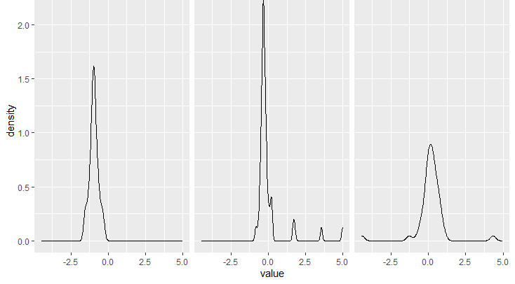
Figure 1: The kernel density function of factor loadings $\bm{b}_{1},\bm{b}_{2},\bm{b}_{3}$ (from left to right respectively) estimated by the PCA method

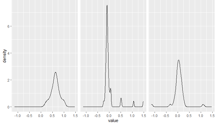
Figure 2: The kernel density function of factor loadings $\bm{b}_{1},\bm{b}_{2},\bm{b}_{3}$ (from left to right respectively) estimated by the PPCA method

The information criterion introduced in (2.14) identifies 9 distinct groups by the PPCA estimators. The details of the membership for all 9 groups of our method and Tu method are reported in the supplement. We then investigate the homogeneity structure among the estimated loading vectors. For better comparison, the Sankey diagram in figure 3 shows the flow of the group membership estimated by our methods to those of Tu and Wang (2023). Our identified group structure has similarities to that identified by TU method. On one hand, the factor loadings for Gold industry and Coal industry are quite different to form a unique group separately. Likewise, the Mines and Oil should be combined in one group. On the other hand, there also exist remarkable distinctions between the grouping structures identified by our method and TU method. For example, our method combined the Cluster1 and Cluster2 of membership estimated by Tu and Wang (2023) into one group. Besides, our method divided the Cluster4 grouped by Tu and Wang (2023) into two groups. Detailed grouping results can be found in the appendix.

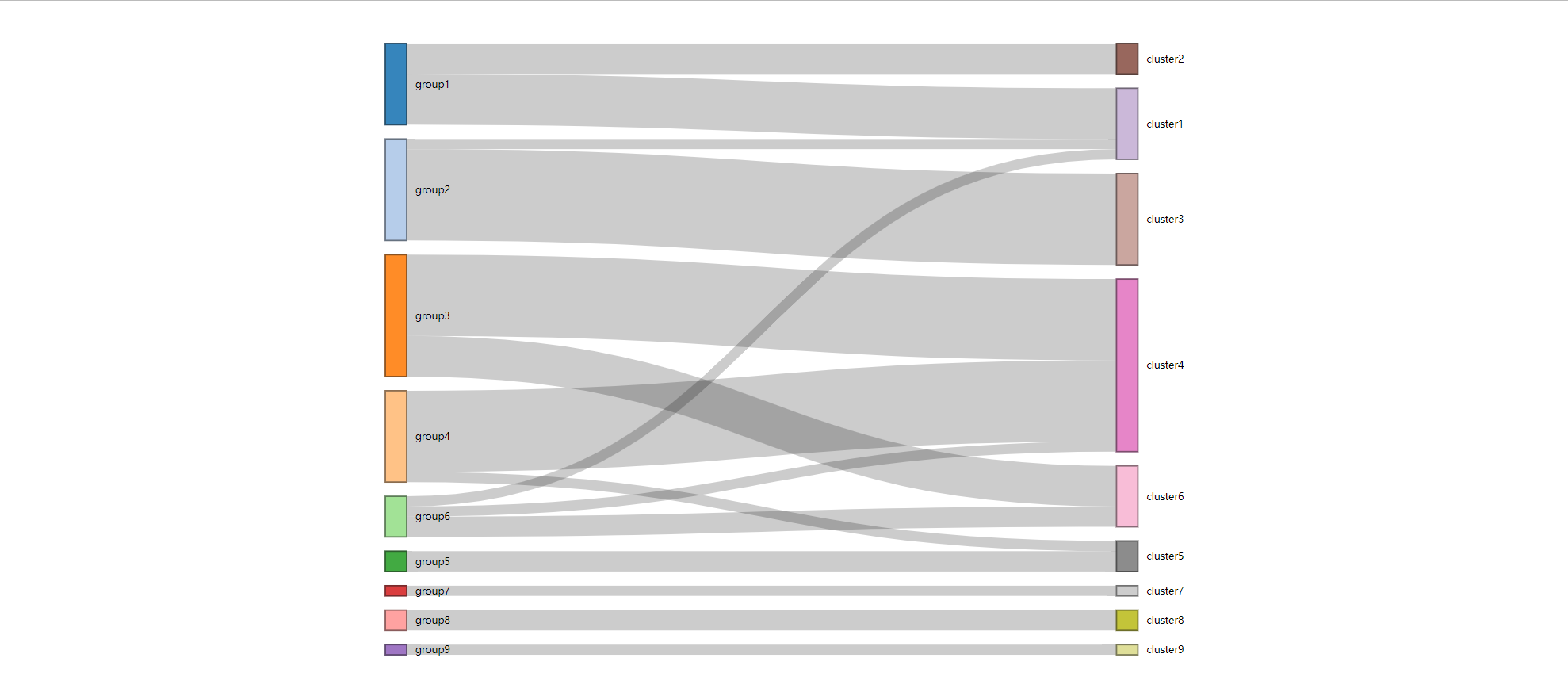
Figure 3: The Sankey diagram: the flows of portfolios from our identified groups (left) to those of Tu and Wang (2023) (right)

Finally, we compare the out-of-sample prediction performance of our proposed method with that of Tu and Wang (2023) for the returns ranging from December 2017 to September 2018. For the accuracy measure, we follow Guo and Li (2022) to use the out-of-sample prediction error(OSPE) of a given month, which is defined as

$$\text{OSPE}=\frac{\sum_{i=1}^{49}\sum_{t\in\tau}(x_{ti}-\widehat{x}_{ti})^{2}}{49\times|\tau|},$$

where $\tau$ denotes the set of days in this month remained after removing the missing values and $\widehat{x}_{ti}$ is the predicted value of the $i$-$th$ series at time $t$-$th$ day of a month by using all data prior to this month. We start with extracting factors from the standardized 49 industry portfolios between January 2016 and November 2017, and then we estimate the homogeneity structure using our proposed method, with which the factors are re-estimated. To forecast the daily returns in December 2017, we use a training set from January 2016 to November 2017 to estimate the loading matrix and then form the forecast with factors estimated from the full sample. Next, to forecast the returns in January 2018, the training set is further augmented with data in December 2017. We continue this process until September 2018, and the OSPEs are sequentially calculated, presented in Table 4, where the OSPE1 represents the OPSE results of Tu, while the OPSE2 represents that of PPCA. From Table 4, we can see that our proposed method always outperforms that of Tu and Wang (2023) for OPSE.

Table 4: OPSE1 and OPSE2 from 2017.12-2018.9

	2017.12	2018.1	2018.2	2018.3	2018.4	2018.5	2018.6	2018.7	2018.8	2018.9
OPSE1	1.8036	1.5782	3.4238	2.7635	2.3107	1.3026	2.0564	1.3511	1.5763	1.4675
OPSE2	1.7761	1.4815	3.4121	2.7463	2.1952	1.2439	1.9313	1.3066	1.4938	1.3973

6 Conclusions and discussions

In this paper, we first propose an PPCA method with $\ell_{2}$-norm penalty for group pursuit under factor model and provide a closed-form solution. We give the asymptotic properties of the PPCA estimators. We further present an AHC approach for estimating the latent homogeneity structure in the loadings. Then we adopt the constrained least squares method to obtain the group-specific loading vectors. We also propose an information criterion to determine the unknown group number. Consistency and asymptotic normality are derived for both the PPCA estimators and the post-grouping estimators under very mild conditions. It is demonstrated that our proposed PPCA method outperforms the PCA method when latent groups exist. We also conclude that the PPCA estimators act as more promising initial values for subsequent clustering procedure. The real data analysis illustrates the practical merits of our methodology.

The current work can be extended in several directions. Firstly, the proposed PPCA method can be used to locate change points in the presence of group structure (Baltagi et al., 2017). Secondly, the matrix factor model (Han et al., 2020, 2022; Chen et al., 2022; Yu et al., 2022; He et al., 2023a, b, 2024a) has been well studied in the literature in the last few years and pursuit for two-way group homogeneity is an interesting and challenging problem. Such extensions deserve separate study and are left as our future work.

References

- Ahn and Horenstein (2013) Ahn, S.C., Horenstein, A.R., 2013. Eigenvalue ratio test for the number of factors. Econometrica 81, 1203–1227.
- Bai (2003) Bai, J., 2003. Inferential theory for factor models of large dimensions. Econometrica 71, 135–171.
- Bai and Li (2012) Bai, J., Li, K., 2012. Statistical analysis of factor models of high dimension. The Annals of Statistics 40, 436 – 465.
- Bai and Li (2016) Bai, J., Li, K., 2016. Maximum likelihood estimation and inference for approximate factor models of high dimension. Review of Economics and Statistics 98, 298–309.
- Bai and Ng (2002) Bai, J., Ng, S., 2002. Determining the number of factors in approximate factor models. Econometrica 70, 191–221.
- Bai and Ng (2006) Bai, J., Ng, S., 2006. Determining the number of factors in approximate factor models, errata. Manuscript, Columbia University .
- Baltagi et al. (2017) Baltagi, B.H., Kao, C., Wang, F., 2017. Identification and estimation of a large factor model with structural instability. Journal of Econometrics 197, 87–100.
- Barigozzi et al. (2024) Barigozzi, M., Cho, H., Maeng, H., 2024. Tail-robust factor modelling of vector and tensor time series in high dimensions. arXiv preprint arXiv:2407.09390 .
- Bates et al. (2013) Bates, B.J., Plagborg-Møller, M., Stock, J.H., Watson, M.W., 2013. Consistent factor estimation in dynamic factor models with structural instability. Journal of Econometrics 177, 289–304.
- Chamberlain and Rothschild (1982) Chamberlain, G., Rothschild, M., 1982. Arbitrage, Factor Structure, and Mean-Variance Analysis on Large Asset Markets. Working Paper 996. National Bureau of Economic Research.
- Chen (2019) Chen, J., 2019. Estimating latent group structure in time-varying coefficient panel data models. The Econometrics Journal 22, 223–240.
- Chen et al. (2021a) Chen, J., Li, D., Wei, L., Zhang, W., 2021a. Nonparametric homogeneity pursuit in functional-coefficient models. Journal of Nonparametric Statistics 33, 387–416.
- Chen et al. (2021b) Chen, L., Dolado, J.J., Gonzalo, J., 2021b. Quantile factor models. Econometrica 89, 875–910.
- Chen et al. (2022) Chen, R., Yang, D., Zhang, C.H., 2022. Factor models for high-dimensional tensor time series. Journal of the American Statistical Association 117, 94–116.
- Fama and French (1992) Fama, E.F., French, K.R., 1992. The cross-section of expected stock returns. The Journal of Finance 47, 427–465.
- Fama and French (1993) Fama, E.F., French, K.R., 1993. Common risk factors in the returns on stocks and bonds. Journal of Financial Economics 33, 3–56.
- Fan et al. (2019) Fan, J., Ke, Y., Sun, Q., Zhou, W., 2019. Farmtest: Factor-adjusted robust multiple testing with approximate false discovery control. Journal of the American Statistical Association 114, 1880–1893.
- Fan et al. (2013) Fan, J., Liao, Y., Mincheva, M., 2013. Large covariance estimation by thresholding principal orthogonal complements. Journal of the Royal Statistical Society Series B: Statistical Methodology 75, 603–680.
- Fan et al. (2015) Fan, J., Liao, Y., Shi, X., 2015. Risks of large portfolios. Journal of Econometrics 186, 367–387.
- Fan et al. (2018) Fan, J., Liu, H., Wang, W., 2018. Large covariance estimation through elliptical factor models. Annals of statistics 46, 1383.
- Forni et al. (2005) Forni, M., Hallin, M., Lippi, M., Reichlin, L., 2005. The generalized dynamic factor model: one-sided estimation and forecasting. Journal of the American statistical Association 100, 830–840.
- Guo and Li (2022) Guo, C., Li, J., 2022. Homogeneity and structure identification in semiparametric factor models. Journal of Business & Economic Statistics 40, 408–422.
- Han and Caner (2017) Han, X., Caner, M., 2017. Determining the number of factors with potentially strong within-block correlations in error terms. Econometric Reviews 36, 946–969.
- Han et al. (2020) Han, Y., Chen, R., Yang, D., Zhang, C., 2020. Tensor factor model estimation by iterative projection. The Annals of Statistics, in press .
- Han et al. (2022) Han, Y., Zhang, C.H., Chen, R., 2022. Rank determination in tensor factor model. Electronic Journal of Statistics 16, 1726–1803.
- He et al. (2023a) He, Y., Kong, X., Trapani, L., Yu, L., 2023a. One-way or two-way factor model for matrix sequences? Journal of Econometrics 235, 1981–2004.
- He et al. (2022) He, Y., Kong, X., Yu, L., Zhang, X., 2022. Large-dimensional factor analysis without moment constraints. Journal of Business & Economic Statistics 40, 302–312.
- He et al. (2023b) He, Y., Kong, X., Yu, L., Zhang, X., Zhao, C., 2023b. Matrix factor analysis: From least squares to iterative projection. Journal of Business and Economic Statistics 42, 322–334.
- He et al. (2024a) He, Y., Kong, X.B., Trapani, L., Yu, L., 2024a. Online change-point detection for matrix-valued time series with latent two-way factor structure. The Annals of Statistics, in press .
- He et al. (2024b) He, Y., Ma, X., Wang, X., Wang, Y., 2024b. Large-dimensional robust factor analysis with group structure. arXiv preprint arXiv:2405.07138 .
- Ma and Tu (2023) Ma, C., Tu, Y., 2023. Group fused lasso for large factor models with multiple structural breaks. Journal of Econometrics 233, 132–154.
- Ma and Huang (2017) Ma, S., Huang, J., 2017. A concave pairwise fusion approach to subgroup analysis. Journal of the American Statistical Association 112, 410–423.
- Ma et al. (2020) Ma, S., Huang, J., Zhang, Z., Liu, M., 2020. Exploration of heterogeneous treatment effects via concave fusion. The International Journal of Biostatistics 16, 20180026.
- Mayrink and Lucas (2013) Mayrink, V.D., Lucas, J.E., 2013. Sparse latent factor models with interactions: Analysis of gene expression data. The Annals of Applied Statistics , 799–822.
- Ross (1977) Ross, S.A., 1977. The capital asset pricing model (capm), short-sale restrictions and related issues. The Journal of Finance 32, 177–183.
- Ross (2013) Ross, S.A., 2013. The arbitrage theory of capital asset pricing, in: Handbook of the fundamentals of financial decision making: Part I. World Scientific, pp. 11–30.
- Shi et al. (2022) Shi, Z., Su, L., Xie, T., 2022. -Relaxation: With Applications to Forecast Combination and Portfolio Analysis. The Review of Economics and Statistics , 1–44.
- Tsai and Tsay (2010) Tsai, H., Tsay, R.S., 2010. Constrained factor models. Journal of the American Statistical Association 105, 1593–1605.
- Tu and Wang (2023) Tu, Y., Wang, B., 2023. On structurally grouped approximate factor models. Manuscript.
- Vogt and Linton (2017) Vogt, M., Linton, O., 2017. Classification of non-parametric regression functions in longitudinal data models. Journal of the Royal Statistical Society Series B: Statistical Methodology 79, 5–27.
- Wang (2022) Wang, F., 2022. Maximum likelihood estimation and inference for high dimensional generalized factor models with application to factor-augmented regressions. Journal of Econometrics 229, 180–200.
- Wang (2012) Wang, H., 2012. Factor profiled sure independence screening. Biometrika 99, 15–28.
- Wang et al. (2018) Wang, W., Phillips, P.C., Su, L., 2018. Homogeneity pursuit in panel data models: Theory and application. Journal of Applied Econometrics 33, 797–815.
- Wang and Zhu (2024) Wang, W., Zhu, Z., 2024. Homogeneity and sparsity analysis for high-dimensional panel data models. Journal of Business & Economic Statistics 42, 26–35.
- Wei et al. (2023) Wei, K., Qin, G., Zhu, Z., 2023. Subgroup analysis for longitudinal data based on a partial linear varying coefficient model with a change plane. Statistics in Medicine 42, 3716–3731.
- Xiang et al. (2023) Xiang, J., Guo, G., Li, J., 2023. Determining the number of factors in constrained factor models via bayesian information criterion. Econometric Reviews 42, 98–122.
- Yu et al. (2022) Yu, L., He, Y., Kong, X., Zhang, X., 2022. Projected estimation for large-dimensional matrix factor models. Journal of Econometrics 229, 201–217.
- Yu et al. (2019) Yu, L., He, Y., Zhang, X., 2019. Robust factor number specification for large-dimensional elliptical factor model. Journal of Multivariate Analysis 174, 104543.
- Yu et al. (2020) Yu, L., He, Y., Zhang, X., Zhu, J., 2020. Network-assisted estimation for large-dimensional factor model with guaranteed convergence rate improvement. arXiv preprint arXiv:2001.10955 .