A spring–block theory of feature learning in deep neural networks

Abstract

A central question in deep learning is how deep neural networks (DNNs) learn features. DNN layers progressively collapse data into a regular low-dimensional geometry. This collective effect of non-linearity, noise, learning rate, width, depth, and numerous other parameters, has eluded first-principles theories which are built from microscopic neuronal dynamics. Here we present a noise–non-linearity phase diagram that highlights where shallow or deep layers learn features more effectively. We then propose a macroscopic mechanical theory of feature learning that accurately reproduces this phase diagram, offering a clear intuition for why and how some DNNs are “lazy” and some are “active”, and relating the distribution of feature learning over layers with test accuracy.

Deep neural networks (DNNs) progressively compute features from which the final layer generates predictions. Something remarkable happens when they are optimized via stochastic dynamics over a data-dependent energy: Each layer learns to compute better features than the previous one [1], ultimately transforming the data to a regular low-dimensional geometry [2, 3, 4, 5]. Feature learning is a striking departure from kernel machines or random feature models (RFM) which compute linear functions of a fixed set of features [6, 7, 8]. How it emerges from microscopic interactions between millions or billions of artificial neurons remains a central open question in deep learning [9, 10, 11, 12, 13].

Existing theories often focus on shallow networks [14, 15, 16, 17], non-feature learning regimes such as the neural tangent kernel (NTK) [18, 19], or linear DNNs [20, 21]. Even with a single hidden layer, the complex interplay of factors like initialization [22], layer width [23], learning rates [24, 25], batch size [26, 27], and dataset properties [28, 29, 30] challenges a statistical mechanics approach to theory building, where feature learning would emerge bottom-up from microscopic interactions. As a result there are scarcely any feature learning theories which address realistic DNNs which are deep and non-linear.

In this paper we rather take a thermodynamical, top-down approach and look for a simplest well-understood phenomenological model which captures the essential aspects of feature learning. We first show that DNNs can be mapped to a phase diagram defined by noise and non-linearity, with phases where layers learn features at equal rates, and where deep or shallow layers learn better features. “Better” is quantified through the notion of data separation—the ratio of feature variance within and across classes. To explain this phase diagram, we propose a macroscopic theory of feature learning in deep, non-linear neural networks: we show that the stochastic dynamics of a non-linear spring–block chain with asymmetric friction fully reproduce the phenomenology of data separation over training epochs and layers. The phase diagram is universal with respect to the source of stochasticity: varying dropout rate, batch size, label noise, or learning rate all result in the same phenomenology.

These findings considerably generalize recent work which showed that in many DNNs each layer improves data separation by the same factor, with surprising regularity [3]. This law of data separation can be proved for linear DNNs with a particular choice of data and initialization [31, 32], but it is puzzling why just as many networks do not abide by it. Fig. 4 illustrates the challenge: the same DNN trained with three different parameter sets results in strikingly different distributions of data separation over layers. Understanding how these non-uniform distributions arise and how it affects generalization is key to understanding feature learning.

Even linear DNNs induce a complex energy landscape and highly non-linear training dynamics [21] that can result in non-even separation. The relationship between the energy landscape and learning has been studied with tools from statistical mechanics [33, 34, 35, 36], random matrix theory [37], and optimal transport [38, 15] but it remains unclear how to connect these insights to macroscopic feature learning in real DNNs.

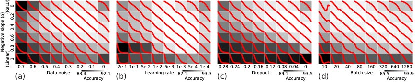
Figure 1: Phase diagrams of DNN load curves (red) for non-linearity v.s. (a) data noise, (b) learning rate, (c) dropout, and (d) batch size. In all cases, noise is strongest on the left, and non-linearity strongest at the top. Background shading encodes test accuracy. Results are averaged over 10 independent runs on MNIST.

In our theory, spring elongations model data separation. The empirical risk exerts a load on the network to which its layers respond by separating the data, subject to non-linearity modeled by friction. Difference in length between consecutive springs gives a load on the incident block. Asymmetric friction models the propagation of signal and noise in forward and backward passes. It models dynamical non-linearity in a network which absorbs load (or spoils signal in gradient) causing the shallow layers to “extend less” (do not learn features). Stochasticity, be it from stochastic gradient descent (SGD) [39, 40], dropout [41], or noisy data [42], reequilibrates the load.

The resulting reproduces the dynamics and the phase diagram of feature learning surprisingly well. It explains when data separation is uniformly distributed across layers but also when deep or shallow layers learn faster. It shows why depth may be problematic for learning and why non-linearity is a double-edged sword, resulting in expressive models but facilitating overfitting. A stability argument suggests a link between generalization and layerwise data separation which we remarkably find true in real DNNs.

Feature learning across layers of DNNs—

A DNN with $L$ hidden layers, weights $\bm{{W}}_{\ell}\in\mathbb{R}^{d_{\ell}\times d_{\ell-1}}$, biases $\bm{{b}}_{\ell}\in\mathbb{R}^{d_{\ell}}$, and activation $\sigma$ maps the input $\bm{{x}}_{0}\equiv\bm{{x}}$ to the output (a label) $\bm{{y}}\equiv\bm{{x}}_{L+1}$ via a sequence of intermediate representations $\bm{{x}}_{0}\to\bm{{x}}_{1}\to\cdots\to\bm{{x}}_{L}\to\bm{{x}}_{L+1}\equiv\bm{{y}}$, where $\bm{{x}}_{L+1}=F(\bm{{x}})=\bm{{W}}_{L+1}\bm{{x}}_{L}+\bm{{b}}_{L+1}$ and

$$\bm{{h}}_{\ell}=\bm{{W}}_{\ell}\bm{{x}}_{\ell-1}+\bm{{b}}_{\ell},\quad\bm{{x}}_{\ell}=c_{\ell}\sigma(\bm{{h}}_{\ell}),$$ (1)

for $\ell=1,\ldots,L$. The activation-dependent normalization factors $c_{\ell}$ scale the variance of hidden features in each layer close to $1$ [43, 44, 45]; they can be replaced by batch normalization [46].

It is natural to expect that in a well-trained DNN the intermediate features $\bm{{x}}_{\ell}$ improve progressively over $\ell$. Following recent work on neural collapse we measure separation as the ratio of variance within and across classes [2, 3, 4, 5, 31]; in supplemental material (SM) [47] we show that analogous phenomenology exists in regression. Let $\mathcal{X}_{\ell}^{k}$ collect the $\ell$th postactivation for examples from class $k$, with $\bar{\bm{{x}}}_{\ell}^{k}$ and $N_{k}$ its mean and cardinality. The between-class and within-class covariances are

$$\Sigma_{\ell}^{\mathrm{w}}:=\operatorname*{Ave}_{k}\,(\mathrm{Cov}\mathcal{X}_{\ell}^{k}),\quad\quad\Sigma_{\ell}^{\mathrm{b}}:=\mathrm{Cov}\left(\tfrac{N_{k}}{N}\bar{\bm{{x}}}_{\ell}^{k}\right)_{k=1}^{K},$$ (2)

where $\mathrm{Ave}$ is the average; $\Sigma^{\mathrm{b}}_{\ell}$ is the between-class “signal” for classification, and $\Sigma^{\mathrm{w}}_{\ell}$ is the within-class variability. Data separation at layer $\ell$ is then defined as

$$D_{\ell}:=\log\left(\mathrm{Tr}\left(\Sigma_{\ell}^{\mathrm{w}}\right)/\mathrm{Tr}\left({\Sigma_{\ell}^{\mathrm{b}}}\right)\right).$$ (3)

The difference $d_{\ell}=D_{\ell-1}-D_{\ell}$ represents the contribution of the $\ell$th layer. We call the “discrete curve” $D_{\ell}$ vs $\ell$ the load curve in anticipation of the mechanical analogy. If indeed each layer improves the representation the load curve should monotonically decrease.

Modern overparameterized DNNs may perfectly fit the training data for different choices of hyperparameters, while yielding different load curves. An extreme is an RFM where only the last layer learns while the rest are frozen at initialization [7, 48]. As the entire load is concentrated on one layer, one might intuitively expect that a more even distribution will result in better performance.

A law of data separation?—

He and Su [3] show that in many well-trained DNNs the load is distributed uniformly over layers,

$$d_{\ell}\approx d_{\ell^{\prime}}\quad\text{for}\quad 1\leq\ell,\ell^{\prime}\leq L,$$

which results in a linear load curve [49]. This can be proved in linear DNNs with orthogonal initialization and gradient flow training [50, 31, 32], but as we show below it is a brittle phenomenon: non-linear activations immediately break the balance. Equiseparation thus requires additional ingredients; He and Su highlight the importance of an appropriate learning rate.

The non-linearity–noise phase diagram—

We show that DNNs define a family of phase diagrams such that (i) increasing non-linearity results in increasingly “concave” load curves, with deeper layers learning better features and thus taking a higher load, $d_{\ell}<d_{\ell^{\prime}}$ for $\ell<\ell^{\prime}$; (ii) adding noise to the dynamics rebalances the load across layers; and (iii) further increasing noise results in convex load curves, with shallower layers learning better features.

We report these findings in Fig. 1. In all panels the abscissa measures stochasticity while the ordinate measures non-linearity. To measure non-linearity we use the slope $\alpha\in[0,1]$ of the negative part of a LeakyReLU activation, $\mathrm{LReLU}(x):=\max(\alpha x,x)$; $\alpha=1$ gives a linear DNN, $\alpha=0$ the ReLU. Consider for example Fig. 1(a) where noise is introduced in labels and data (we randomly reset a fraction $p$ of the labels $\mathbf{y}$, and add Gaussian noise with variance $p^{2}$ to $\bm{{x}}_{0}$). Without noise (upper right corner), the load curve is concave; this resembles an RFM or a kernel machine. Increasing noise (right to left) yields a linear and then a convex load curve.

Interestingly, the same phenomenology results from varying learning rate, dropout, and batch size (Fig. 1(b, c, d)). Lower learning rate, smaller dropout, and larger batch size all indicate less stochasticity in dynamics. Martin and Mahoney [51] call them temperature-like parameters in the statistical mechanics sense; see also Zhou et al. [52]. In all cases high non-linearity and low noise result in “lazy” training [53] and a concave load curve. Low non-linearity and high noise (bottom-left) result in convex load curves. This phenomenology is at the heart of feature learning. It asks how we go from non-feature learning models like RFM or NTK (where only or mostly deep layers learn) to models where all layers learn.

A spring–block theory of feature learning—

We now show something surprising: the complete phenomenology of feature learning, as seen through layerwise data separation, can be reproduced by the stochastic dynamics of a simple spring–block chain. As in Fig. 2, we interpret $d_{\ell}$, the signed elongation of the $\ell$th Hookean spring, as data separation afforded by the $\ell$th layer. Block movement is impeded by friction which models the effect of dynamical non-linearity on gradients; noise in the force models stochasticity from mini-batching, dropout, or elsewhere.

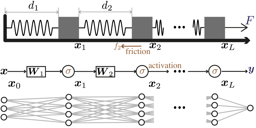
Figure 2: An illustration of the analogy between a spring–block chain and a deep neural network.

The equation of motion for the position of the $\ell$th block, $x_{\ell}=\sum_{i=1}^{\ell}d_{i}$, ignoring block widths, is

$$\ddot{x}_{\ell} =k(x_{\ell+1}-2x_{\ell}+x_{\ell-1})-\gamma\dot{x}_{\ell}+f_{\ell}+\varepsilon\xi_{\ell},$$ (4)

for $\ell=1,\ldots,L$, where we assumed unit masses, $k$ is the elastic modulus, $\gamma$ a linear damping coefficient sufficiently large to avoid oscillations, and $\xi_{\ell}$ is noise such that $\langle\xi_{\ell}(t)\xi_{\ell}(s)\rangle=\delta(t-s)$. As DNNs at initialization do not separate data we let $x_{\ell}(0)=0$. The dynamics is driven by force applied to the last block $F=k(y-x_{L})$. We set $x_{0}\equiv 0$ and $x_{L+1}\equiv y$ to model training data and targets. The load curve plots the distance of the $\ell$th block from the target $D_{\ell}=y-x_{\ell}$. It reflects how much the $\ell$th spring—or the $\ell$th layer—contributes to “explaining” the total extension—or the total data separation. One key insight is that the friction must be asymmetric to model the propagation of noise during training as we elaborate below. We set the sliding and maximum static friction to $\mu_{\rightarrow}$ for rightward and $\mu_{\leftarrow}$ for leftward movement. In this model the friction acts on noisy force. If noise is added to the velocity independently of the friction we obtain a more standard Langevin dynamics. Although this is physically less realistic it shows similar qualitative behavior (for additional details see SM [47]).

The spring–block dynamics of data separation in DNNs—

We now show experimentally and analytically that the proposed model results in a phenomenology analogous to that of data separation in real networks. Indeed, there is a striking similarity between the phase diagram of the spring–block model in Fig. 3 and the DNN phase diagrams in Fig. 1. Surprisingly, it is not only the equilibria of the two systems that are similar, but also the stochastic dynamics; we show this in Fig. 4.

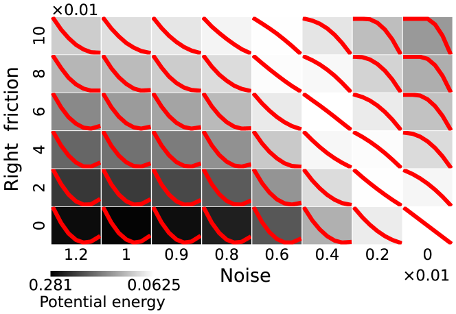
Figure 3: Phase diagram of the spring–block system (5) for friction $\mu_{\rightarrow}$ v.s. noise level $\epsilon$. We set $k=1,\mu_{\leftarrow}=0.2$ and $L=7$. The load curves ($D_{\ell}=y-x_{\ell}$) are recorded at $t=100$; the shading corresponds to the elastic potential energy.

1: Non-linearity breaks the separation balance.

Let us first analyze how our model explains concave load curves and lazy training. For simplicity we work in the overdamped approximation $\gamma\gg 1$; in SM [47] we show that the second order system has the same qualitative behavior. Scaling time by $\gamma$, Eq. (4) then yields

$$\dot{x}_{\ell}=\sigma\big{(}k\,(\bm{L}x)_{\ell}+\varepsilon\xi_{\ell}\big{)}$$ (5)

where $(\bm{L}x)_{\ell}:=x_{\ell+1}-2x_{\ell}+x_{\ell-1}$ and

$$\sigma(z) =\begin{cases}0&\text{~{}if~{}}-\mu_{\leftarrow}\leq z\leq\mu_{\rightarrow}\\ z-\mu_{\rightarrow}&\text{~{}if~{}}z>\mu_{\rightarrow}\\ z+\mu_{\leftarrow}&\text{~{}if~{}}z<-\mu_{\leftarrow}\\ \end{cases}.$$ (6)

Without noise and friction ($\varepsilon=0$, $\mu_{\leftarrow}=\mu_{\rightarrow}=0$) the system is linear with the trivial unique equilibrium $d_{\ell}^{*}\equiv y/(L+1)$ for all $\ell$, which corresponds to the state of lowest elastic potential energy. However, analyzing the resulting system of ODEs shows that adding friction in (5) immediately breaks the symmetry and results in an unbalanced equilibrium,

$$x_{\ell}^{*}=\frac{y\ell}{L+1}-\frac{\mu_{\rightarrow}}{k}\left(\frac{L\ell}{2}-\frac{\ell\left(\ell-1\right)}{2}\right)$$ (7)

if we assume the initial elastic potential $k(y-x_{0})^{2}/2$ is sufficiently large such that all blocks will eventually move. In this case $\Delta d^{*}_{\ell}:=d^{*}_{\ell+1}-d^{*}_{\ell}=(\bm{{L}}x^{*})_{\ell}={\mu_{\rightarrow}}/{k}>0$ and the load curve is concave. Note that this result only involves $\mu_{\rightarrow}$ but not $\mu_{\leftarrow}$ as without noise and with sufficient damping the blocks only move to the right. The interpretation is that in equilibrium, the friction at each block absorbs some of the load so that the shallower springs extend less; in a DNN this corresponds to lazy training where the deepest layer, whose gradients do not experience non-linearity, does most of the separation.

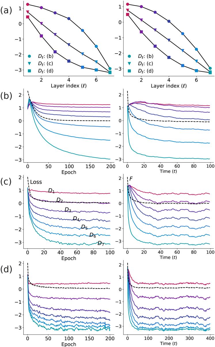
Figure 4: The load curves at convergence (a) and trajectories (b, c, d) for an $7-$hidden layer ReLU fully connected DNN on MNIST (left) and the proposed spring–block model (right). For the DNN (left), the ordinate is $D_{\ell}$ (data separation at layer $\ell$); the dashed line is the training loss. Characteristic behaviors: (b) high non-linearity (high friction) and low randomness in training (noise in force); (c): balanced non-linearity (friction) and randomness (force noise); (d) low non-linearity (friction) and large training randomness (force noise). In the spring system (right), the ordinate represents the distance to the target $D_{\ell}=y-x_{\ell}$ for colored lines. These values are scaled to match the same regime used in the DNN for visualization purposes. The dashed line represents the force at the rightmost block $F$ which is at a different scale from $D_{\ell}$.

2: Noise reequilibrates the load.

If friction reduces load, how can then a chain with friction—or a non-linear DNN—result in a uniformly distributed load? We know from Fig. 1 that in DNNs stochastic training helps achieve this. We now show how our model reproduces this behavior and in particular a counterintuitive phenomenon in Fig. 1 where large noise results in convex load curves where shallow layers learn better than deep. We show that this happens when $\mu_{\leftarrow}>\mu_{\rightarrow}$.

We begin by defining the effective friction over a time window of length $\eta$. Let $\overline{\varepsilon}:=\varepsilon/\sqrt{\eta}$ and $\zeta_{t}\sim(\xi_{t+\eta}-\xi_{t})/\sqrt{\eta}$ (iid). We will assume for convenience that the increments $\zeta$ are bounded (see SM [47] for details). The effective friction is then

$$\mu_{\text{eff}}:=\text{E}_{\zeta}\big{[}\left(\sigma(k\Delta d+\overline{\varepsilon}\zeta)-k\Delta d\right)\mid\sigma(k\Delta d+\overline{\varepsilon}\zeta)\neq 0\big{]}.$$

For large noise we will have that $\mu_{\text{eff}}\approx\lim_{\overline{\varepsilon}\to\infty}\mu_{\text{eff}}=\frac{1}{2}(\mu_{\rightarrow}-\mu_{\leftarrow})$. Since this effective friction is approximately independent of $x$, the load curve can be approximated by substituting $\mu_{\text{eff}}$ for $\mu_{\rightarrow}$ in Eq. (7), which leads to

$$\Delta d^{*}\approx\frac{1}{k}\lim_{\overline{\varepsilon}\to\infty}\mu_{\text{eff}}(\overline{\varepsilon})=\frac{\mu_{\rightarrow}-\mu_{\leftarrow}}{2k}.$$ (8)

It is now clear that with sufficient noise the load curve is concave if $\mu_{\rightarrow}>\mu_{\leftarrow}$, linear if $\mu_{\rightarrow}=\mu_{\leftarrow}$, and convex if $\mu_{\rightarrow}<\mu_{\leftarrow}$. We can also see that for $\overline{\varepsilon}=0$, $\mu_{\text{eff}}=\mu_{\rightarrow}$, so that this effective friction correctly generalizes the noiseless case Eq. (7) and we have that $\Delta d^{*}\in[\frac{\mu_{\rightarrow}-\mu_{\leftarrow}}{2k},\frac{\mu_{\rightarrow}}{k}]$.

Further, when $\Delta d\in[\frac{\mu_{\rightarrow}-\mu_{\leftarrow}}{2k},\frac{\mu_{\rightarrow}}{k}]$, it holds that $\frac{\mathrm{d}\mu_{\text{eff}}}{\mathrm{d}\varepsilon}\leq 0$. It implies that increasing noise always decreases effective friction which resembles phenomena like acoustic lubrication or noise-induced superlubricity [54]. When $\mu_{\leftarrow}>\mu_{\rightarrow}>0$, as we vary $\varepsilon$ from $0$ to $\infty$ we will first see a concave, then a linear, and finally a convex load curve, corresponding to the transition from lazy to active training in DNNs [53]. As a result, when $\mu_{\leftarrow}>\mu_{\rightarrow}>0$ our model explains the entire DNN phase diagram.

How can we relate the condition $\mu_{\leftarrow}>\mu_{\rightarrow}>0$ to DNN phenomenology? Note that in our model $\mu_{\leftarrow}$ is activated only due to the noise, since the signal (the pulling force) is always to the right. In a DNN, the forward pass of the backpropagation algorithm computes the activations while the backward pass computes the gradients and updates the weights. In the forward pass, the input is multiplied by the weight matrices starting from the shallowest to the deepest. With noise (e.g. dropout), the activations of the deepest layer accumulate the largest noise. Thus noise in DNN training chiefly propagates from shallow to deep. This is exactly what $\mu_{\leftarrow}>\mu_{\rightarrow}$ in our model implies, since $\mu_{\leftarrow}$ is only triggered by noise.

Indeed, from Eq. (8) we see that when only friction for leftward move is present, $\mu_{\leftarrow}>\mu_{\rightarrow}=0$, the load curve is convex if $\varepsilon>0$ and linear if $\varepsilon=0$ (Fig. 5(b)). This equilibrium is independent of $\mu_{\leftarrow}$ since no block moves left. This observation parallels findings in linear DNNs where training with gradient flow and “whitened” data leads to a linear load curve [31]. In contrast, introducing dropout or large learning rate makes the load curve convex (Fig. 5(a)). This shows that dynamical non-linearity—or friction in our model—exists even in linear DNNs, so that their learning dynamics are non-linear [21].

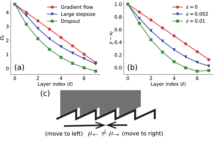
Figure 5: (a) Load curve of a deep linear neural network on random orthonormal datasets. (b) Spring–block model without left friction ($\mu_{\rightarrow}=0$) with $\mu_{\leftarrow}=0.1$, under varying levels of noise $\varepsilon$. (c) An illustration of asymmetric friction.

3: Equiseparation minimizes elastic potential energy and improves generalization—

We finally give an example of how the proposed theory yields practical insights. Among all spring–block chains under a fixed load, the equiseparated one is the most stable in the sense of having the lowest potential energy. This motivates us to look at the test accuracy of DNNs as a function of load curve curvature; this is shown as background shading in Fig. 1. The result is intriguing: Linear load curves correspond to the highest test accuracy. It suggests that by balancing non-linearity with noise, DNNs are at once highly expressive and not overfitting.

That a uniform load distribution yields the best performance is intuitively pleasing. It is also valuable operationally as it may help guide training to find better networks. In Fig. 6, we illustrate an experiment where we first train a CNN using Adam [55] at a learning rate of $10^{-4}$. The training nearly converges after $20\times 200$ epochs, resulting in a concave load curve (purple). Motivated by the above finding, we may try to linearize the load curve. A $5\%$ dropout causes the training to resume and the load curve to become linear (blue). Importantly, it improves accuracy. Higher noise (a $30\%$ dropout at $40\times 200$ epochs) gives a convex load curve and worse generalization.

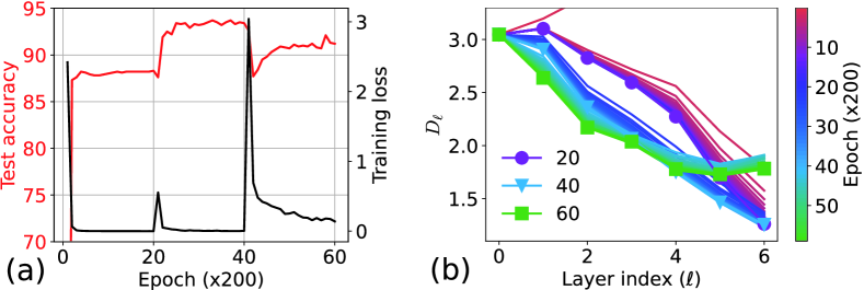
Figure 6: The dynamics of load curves for a deep convolution network (CNN) on FashionMNIST dataset. (a) test accuracy versus training loss. (b) the corresponding load curves during training. In the experiments, we introduce $5\%$ at epoch $20\times 200$ and $30\%$ dropout at epoch $40\times 200$.

Conclusion—

Deep learning theories are primarily built bottom-up, by analyzing the collective behavior of the myriad artificial neurons interacting in a data-driven energy from first principles. But fields like physics, biology, neuroscience, and economics, which have long dealt with comparable complexity (or, sometimes, worse) have long benefitted from both bottom-up and top-down, phenomenological approaches. We think that deep learning can similarly benefit from both paradigms. Our study attempts to introduce a simple phenomenological model to help understand feature learning—an essential aspect of modern real-world DNNs which requires us to simultaneously consider depth, non-linearity, and noise, something that at the moment seems to be out of reach of the bottom-up paradigm. It is a priori not obvious that such a model exists: it requires identifying a suitable low-dimensional description of the system and demonstrating its approximately autonomous behavior. Inspired by a series of works on neural collapse and data separation, our theory elucidates the role of non-linearity and randomness and suggests exciting connections with generalization and conjectures that are worth pursuing rigorously. Analogies such as spring-block models have historically played important roles across science; a prime example is the Burridge–Knopoff model in seismology [56] and related ideas in neuroscience [57]. We find it intriguing that a simple phenomenological model holds significant explanatory power for realistic DNNs, serving as a valuable tool for applying intuitive physical insights to complex, abstract objects. In closing, we mention that we initially considered various cascade structures from daily life as possible analogies to DNNs. For amusing videos involving a folding ruler, see the SM [47].

A spring–block theory of feature learning in deep neural networks
SUPPLEMENTAL MATERIAL

I S1. A folding ruler experiment

We describe an experiment showing that another cascade structure, a folding ruler, may anecdotally serve as a DNN analogy. The goal of the experiment is to show that noise can renegotiate the imbalance caused by friction. As shown in Fig. S1, we pin the left end of the folding ruler and pull the right end by hand. Due to friction, if we pull it very slowly and steadily, the outer layer extends far while the inner layers are close to stuck. This reminds us of lazy training where the outer layers take the largest proportion of the load. Conversely, shaking while pullings helps “activate” the inner layers and redistribute the force, and ultimately results in a uniformly distributed extension of each layer. Videos can be found at https://github.com/DaDaCheng/DNN_Spring

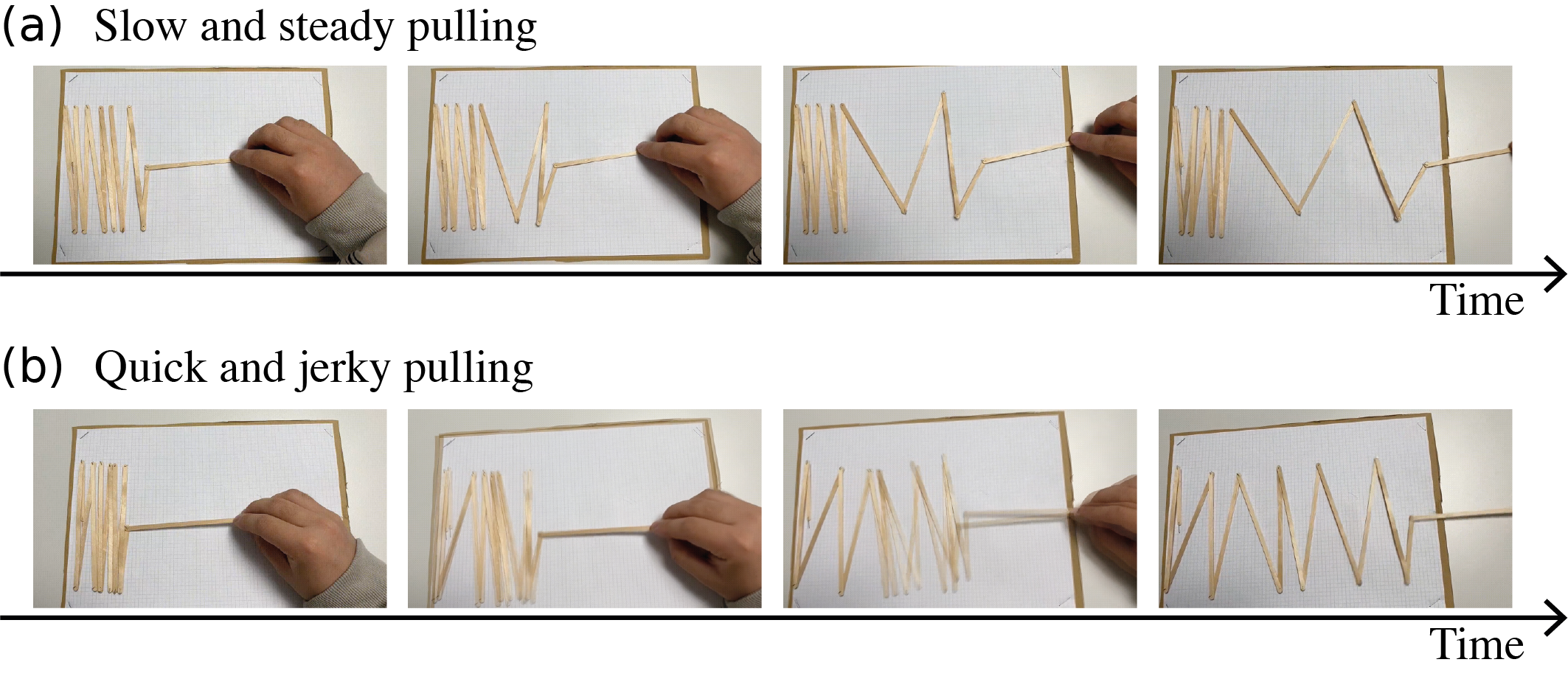
Figure S1: Two ways to extend a folding ruler: (a) With slow and steady pulling, the outer layer extends more than the inner layer due to friction. (b) With quick and jerky pulling, the “active” dynamics redistribute the extension across the different layers.

II S2. Details of numerical experiments and reproducibility

In Figs. 1, 4, and S2, the networks are $8$-layer fully connected MLPs (7 hidden layers), with layer width equal to $100$. We use ReLU activations, BatchNorm in each layer, and no dropout unless stated otherwise. All parameters are initialized using the default settings in PyTorch. The networks are trained using the ADAM optimizer on 2560 training samples from the MNIST dataset, with cross-entropy loss for classification tasks. Unless otherwise specified, the learning rate is set to 0.001 and the batch size is 2560. The test accuracy is measured on the entire 10,000-sample test dataset after training 100 epochs. Notably, when we replace BatchNorm with the scaling constant $c_{\ell}$ mentioned in the main text, we still observe similar convex–concave patterns in the phase diagram corresponding to noise and non-linearity. However, without the adaptive BatchNorm, the load curves exhibit more fluctuations and are less smooth. Additionally, the variations between independent runs become more pronounced.

In the left column of Fig. 4, we train the described DNN with learning rate of 0.0001 and batch size of 200 in panel (b); learning rate of 0.001, dropout of 0.1 and batch size of 100 in panel (c); learning rate of 0.003, and batch size of 50, and dropout of 0.2 in panel (d). In the right column we set $k=1,y=1$ for all three cases, and $\mu_{\rightarrow}=0.11,\mu_{\leftarrow}=0.03$ and $\varepsilon=0.006$ for (b); $\mu_{\rightarrow}=\mu_{\leftarrow}=0.04$ and $\varepsilon=0.01$ for (c); $\mu_{\rightarrow}=0.04,\mu_{\leftarrow}=0.12$ and $\varepsilon=0.011$ for (d). These parameters are chosen to produce qualitatively similar curves with the previous three characteristic training dynamics. For the spring experiments in Fig. 4, we use the same noise for all blocks $\xi_{\ell}(t)=\xi_{\ell^{\prime}}(t)$, to mimic the training of DNNs in which the randomness (e.g., data noise, learning rate, and batch size) in each layer are not independent. This synchronous noise results in more similar dynamics over epochs (in particular the fluctuations) but ultimately leads to similar load curves as independent noise as shown in Fig. 2.

In Fig. 5(a), we adopt the setting from [31]. We use SGD (instead of ADAM) with learning rate of 0.001 to train a linear DNN. All weight matrices are initialized as random orthogonal matrices; the data is also a random orthogonal matrix with random binary labels. There is no batch normalization. We set the learning rate to $0.01$ to generate the “large stepsize” result (blue curve) and apply $10\%$ dropout to generate the “dropout” results (green curve).

In Fig. 6, we consider a CNN with 16 channels and 7 convolutional layers on the Fashion-MNIST dataset. We use ReLU activations and BatchNorm between the convolutional layers. Pooling and linear layers are applied only after the final convolutional layer. All experiments are reproducible using code at https://github.com/DaDaCheng/DNN_Spring.

III S3. Regression

The same phenomenology described in the main text for classification can also be observed for regression if we define the load as the MSE (or RMSE) of the optimal linear regressor from the $\ell$th layer features,

$$D_{\ell}:=\sqrt{\min_{\bm{{w}},\bm{{b}}}\frac{1}{2N}\sum_{(\bm{{x}}_{\ell},\bm{{y}})}\|\bm{{y}}-\bm{{w}}^{\top}\bm{{x}}_{\ell}+\bm{{b}}\|^{2}_{2}},$$

where $N$ is the number of data pairs and the summation is taken over all data. As shown in Fig. S2, noisier training results in a convex load curve, whereas lazy training results in a concave curve.

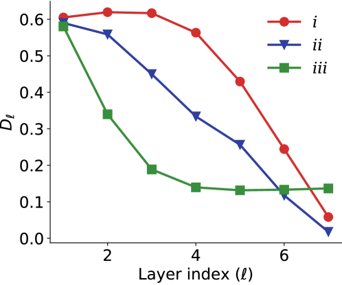
Figure S2: Regression load curve on Diabetes dataset [58] for a 7 hidden-layer ReLU network. (i) learning rate of 0.001 without dropout. (ii) learning rate of 0.01 without dropout (iii) learning rate of 0.02 and with 30% dropout.

IV S4. Additional details about the spring block systems

IV.1 Friction in the second order system

To build intuition about the second order system dynamics (4), we can rewrite it as

$$F_{\ell} =k(x_{\ell+1}-2x_{\ell}+x_{\ell-1})-\gamma v_{\ell}+\varepsilon\xi_{\ell},$$ (9)

$$\ddot{x}_{\ell} =F_{\ell}+f_{\ell}=\sigma(F_{\ell};\dot{x}_{\ell})$$

where the friction $f_{\ell}$ depends on the force $F_{\ell}$ and the velocity $\dot{x}_{\ell}$. If a block is moving to the right ($\dot{x}_{\ell}>0$), sliding friction resists its movement as $f_{\ell}=-\mu_{\rightarrow}$. If a block is moving to the left ($\dot{x}_{\ell}<0$), sliding friction is $f_{\ell}=\mu_{\leftarrow}$. When a block is stationary ($\dot{x}=0$), static friction compensates for all other forces as long as they do not exceed the maximum static friction, i.e., $f_{\ell}=-F_{\ell}$ when $-\mu_{\leftarrow}\leq F_{\ell}\leq\mu_{\rightarrow}$. We take the maximum static friction to be equal to the sliding friction to simplify the model. We can summarize the above cases in an activation-like form,

$$\sigma(z;\dot{x}) =\begin{cases}0&\text{~{}if~{}}\dot{x}=0\text{~{}and~{}}-\mu_{\leftarrow}\leq z\leq\mu_{\rightarrow}\\ z-\mu_{\rightarrow}&\text{~{}if~{}}\dot{x}>0\text{~{}or~{}}(\dot{x}=0\text{~{}and~{}}z>\mu_{\rightarrow})\\ z+\mu_{\leftarrow}&\text{~{}if~{}}\dot{x}<0\text{~{}or~{}}(\dot{x}=0\text{~{}and~{}}z<-\mu_{\leftarrow}).\\ \end{cases}$$ (10)

The phase diagram of this second order system is shown in Fig S3.

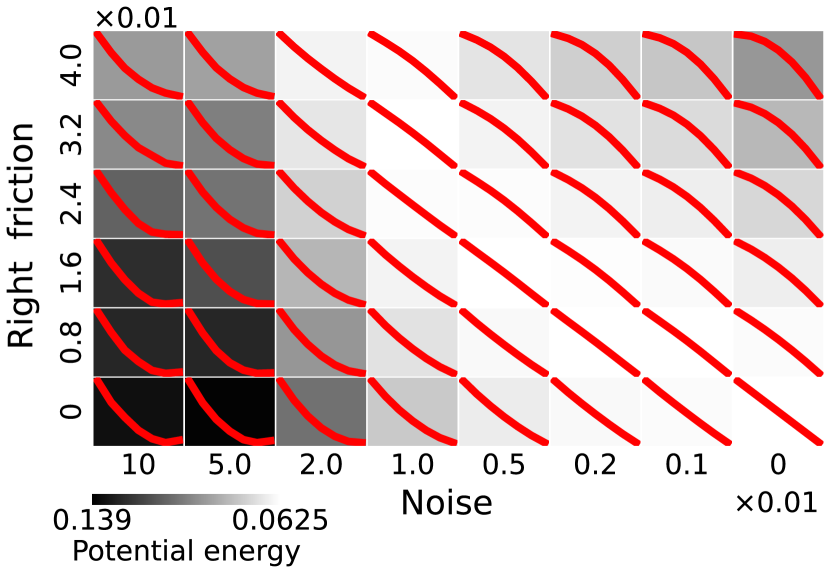
Figure S3: Phase diagram of the second order spring block system (4) for friction $\mu_{\rightarrow}$ v.s. noise level $\epsilon$. We set $k=\gamma=1,\mu_{\leftarrow}=0.12$ and $L=7$. Red load curves ($D_{\ell}=y-x_{\ell}$) are recorded at $t=100$; the shading corresponds to the elastic potential energy.

IV.2 Noisy equilibiria and separation of time scales

In the main text, we mentioned that it is convenient to assume bounded (zero-mean, symmetric) noise increments, for example by using a truncated Gaussian distribution. Without truncation, the trajectories of the spring–block system exhibit two stages. In the first stage, the elastic force dominates the Gaussian tails and the block motion is primarily driven by the (noisy) spring force. At the end of this period, the spring force is balanced with friction. At this point the blocks can only move due to a large realization of noise. These low-probability realizations will move the blocks very slowly close to the equilibrium $\Delta d^{*}=\frac{\mu_{\rightarrow}-\mu_{\rightarrow}}{2k}$ which is stable under symmetric noise perturbations. This is undesirable for analysis since this stable point does not depend on the noise level; in particular, it will be eventually reached even for arbitrarily small $\varepsilon$. This, however, will happen in an exponentially long time, longer than $e^{c_{0}/\epsilon^{2}}$ for some constant $c_{0}$. We can obviate this nuisance in three natural ways: by assuming bounded noise incremenents, by applying noise decay, or by introducing a stopping criterion, for example via a relative change threshold. All are well-rooted in DNN practice: common noise sources are all bounded, and standard training practices involve a variety of parameter scheduling and stopping criteria.

IV.3 Second order Langevin equation

We can obtain a more standard Langevin dynamics formulation of Eq. (9) by adding noise to the velocity independently of the friction, i.e., computing the friction before adding noise. We note that this is less realistic from a physical point of view. The position of the $\ell$th block $x_{\ell}=\sum_{i=1}^{\ell}d_{i}$ then obeys the equation of motion $\mathrm{d}x=v\mathrm{d}t$ with

$$\mathrm{d}v_{\ell}=\left(k(\bm{L}x)_{\ell}-f(v_{\ell})-\gamma v_{\ell}\right)\mathrm{d}t+\varepsilon(t)\mathrm{d}W_{\ell}(t),$$ (11)

where the sliding friction $f$ resists movement as

$$f(v)=\begin{cases}\mu_{\rightarrow}&\text{if~{}}v>0\\ -\mu_{\leftarrow}&\text{if~{}}v<0.\end{cases}$$ (12)

In Eq. (11), $W_{\ell}(t)$ represents the Wiener process with $\varepsilon$ controlling the amount of the noise (temperature parameters). To ensure convergence in this formulation we have to decay the noise; we set $\varepsilon(t)=\varepsilon_{0}e^{-\tau t}$. The friction at zero speed $f(0)$ is defined similarly to the static friction $f_{\ell}$ in Eq. 9, but with $F_{\ell}=k(\bm{{L}}x)_{\ell}$ without considering noise. This dynamics can be solved by standard SDE integration. It results in a similar phase diagram at convergence, as shown in Fig S4, although the fluctuations do not appear as similar as with the formulation in the main text.

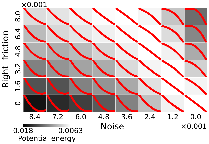
Figure S4: Phase diagram of spring block system with Langevin equation (11) for friction $\mu_{\rightarrow}$ v.s. noise level $\epsilon_{0}$. We set $k=0.1,\gamma=1,\tau=0.002,\mu_{\leftarrow}=0.016$ and $L=7$. Red load curves ($D_{\ell}=y-x_{\ell}$) are recorded at $t=300$; the shading corresponds to the elastic potential energy.

References

- Zeiler and Fergus [2014] M. D. Zeiler and R. Fergus, Visualizing and understanding convolutional networks, in Computer Vision–ECCV 2014: 13th European Conference, Zurich, Switzerland, September 6-12, 2014, Proceedings, Part I 13 (Springer, 2014) pp. 818–833.
- Papyan et al. [2020] V. Papyan, X. Han, and D. L. Donoho, Prevalence of neural collapse during the terminal phase of deep learning training, Proceedings of the National Academy of Sciences 117, 24652 (2020).
- He and Su [2023] H. He and W. J. Su, A law of data separation in deep learning, Proceedings of the National Academy of Sciences 120, e2221704120 (2023).
- Zarka et al. [2021] J. Zarka, F. Guth, and S. Mallat, Separation and concentration in deep networks, in ICLR 2021-9th International Conference on Learning Representations (2021).
- Rangamani et al. [2023] A. Rangamani, M. Lindegaard, T. Galanti, and T. A. Poggio, Feature learning in deep classifiers through intermediate neural collapse, in International Conference on Machine Learning (PMLR, 2023) pp. 28729–28745.
- Hofmann et al. [2008] T. Hofmann, B. Schölkopf, and A. J. Smola, Kernel methods in machine learning, The Annals of Statistics 36, 1171 (2008).
- Rahimi and Recht [2007] A. Rahimi and B. Recht, Random features for large-scale kernel machines, Advances in neural information processing systems 20 (2007).
- Daniely et al. [2016] A. Daniely, R. Frostig, and Y. Singer, Toward deeper understanding of neural networks: The power of initialization and a dual view on expressivity, Advances in neural information processing systems 29 (2016).
- Radhakrishnan et al. [2024] A. Radhakrishnan, D. Beaglehole, P. Pandit, and M. Belkin, Mechanism for feature learning in neural networks and backpropagation-free machine learning models, Science 383, 1461 (2024).
- Lou et al. [2022] Y. Lou, C. E. Mingard, and S. Hayou, Feature learning and signal propagation in deep neural networks, in International Conference on Machine Learning (PMLR, 2022) pp. 14248–14282.
- Baratin et al. [2021] A. Baratin, T. George, C. Laurent, R. D. Hjelm, G. Lajoie, P. Vincent, and S. Lacoste-Julien, Implicit regularization via neural feature alignment, in International Conference on Artificial Intelligence and Statistics (PMLR, 2021) pp. 2269–2277.
- Yang and Hu [2021] G. Yang and E. J. Hu, Tensor programs IV: Feature learning in infinite-width neural networks, in International Conference on Machine Learning (PMLR, 2021) pp. 11727–11737.
- Chizat and Netrapalli [2023] L. Chizat and P. Netrapalli, Steering deep feature learning with backward aligned feature updates, arXiv preprint arXiv:2311.18718 (2023).
- Mei et al. [2018] S. Mei, A. Montanari, and P.-M. Nguyen, A mean field view of the landscape of two-layer neural networks, Proceedings of the National Academy of Sciences 115, E7665 (2018).
- Chizat and Bach [2018] L. Chizat and F. Bach, On the global convergence of gradient descent for over-parameterized models using optimal transport, Advances in neural information processing systems 31 (2018).
- Wang et al. [2021] Y. Wang, J. Lacotte, and M. Pilanci, The hidden convex optimization landscape of regularized two-layer relu networks: an exact characterization of optimal solutions, in International Conference on Learning Representations (2021).
- Arnaboldi et al. [2023] L. Arnaboldi, L. Stephan, F. Krzakala, and B. Loureiro, From high-dimensional & mean-field dynamics to dimensionless odes: A unifying approach to sgd in two-layers networks, in The Thirty Sixth Annual Conference on Learning Theory (PMLR, 2023) pp. 1199–1227.
- Jacot et al. [2018] A. Jacot, F. Gabriel, and C. Hongler, Neural tangent kernel: Convergence and generalization in neural networks, Advances in neural information processing systems 31 (2018).
- Arora et al. [2019] S. Arora, S. S. Du, W. Hu, Z. Li, R. R. Salakhutdinov, and R. Wang, On exact computation with an infinitely wide neural net, Advances in neural information processing systems 32 (2019).
- Arora et al. [2018a] S. Arora, N. Cohen, N. Golowich, and W. Hu, A convergence analysis of gradient descent for deep linear neural networks, arXiv preprint arXiv:1810.02281 (2018a).
- Li and Sompolinsky [2021] Q. Li and H. Sompolinsky, Statistical mechanics of deep linear neural networks: The backpropagating kernel renormalization, Physical Review X 11, 031059 (2021).
- Luo et al. [2021] T. Luo, Z.-Q. J. Xu, Z. Ma, and Y. Zhang, Phase diagram for two-layer relu neural networks at infinite-width limit, Journal of Machine Learning Research 22, 1 (2021).
- Maillard et al. [2023] A. Maillard, A. S. Bandeira, D. Belius, I. Dokmanić, and S. Nakajima, Injectivity of relu networks: perspectives from statistical physics, arXiv preprint arXiv:2302.14112 (2023).
- Cui et al. [2024] H. Cui, L. Pesce, Y. Dandi, F. Krzakala, Y. M. Lu, L. Zdeborová, and B. Loureiro, Asymptotics of feature learning in two-layer networks after one gradient-step, arXiv preprint arXiv:2402.04980 (2024).
- Sohl-Dickstein [2024] J. Sohl-Dickstein, The boundary of neural network trainability is fractal, arXiv preprint arXiv:2402.06184 (2024).
- Marino and Ricci-Tersenghi [2024] R. Marino and F. Ricci-Tersenghi, Phase transitions in the mini-batch size for sparse and dense two-layer neural networks, Machine Learning: Science and Technology 5, 015015 (2024).
- Dandi et al. [2024] Y. Dandi, E. Troiani, L. Arnaboldi, L. Pesce, L. Zdeborová, and F. Krzakala, The benefits of reusing batches for gradient descent in two-layer networks: Breaking the curse of information and leap exponents, arXiv preprint arXiv:2402.03220 (2024).
- Ben Arous et al. [2022] G. Ben Arous, R. Gheissari, and A. Jagannath, High-dimensional limit theorems for sgd: Effective dynamics and critical scaling, Advances in Neural Information Processing Systems 35, 25349 (2022).
- Boursier and Flammarion [2024] E. Boursier and N. Flammarion, Early alignment in two-layer networks training is a two-edged sword, arXiv preprint arXiv:2401.10791 (2024).
- Goldt et al. [2020] S. Goldt, M. Mézard, F. Krzakala, and L. Zdeborová, Modeling the influence of data structure on learning in neural networks: The hidden manifold model, Physical Review X 10, 041044 (2020).
- Yaras et al. [2023] C. Yaras, P. Wang, W. Hu, Z. Zhu, L. Balzano, and Q. Qu, The law of parsimony in gradient descent for learning deep linear networks, arXiv preprint arXiv:2306.01154 (2023).
- Wang et al. [2023] P. Wang, X. Li, C. Yaras, Z. Zhu, L. Balzano, W. Hu, and Q. Qu, Understanding deep representation learning via layerwise feature compression and discrimination, arXiv preprint arXiv:2311.02960 (2023).
- Gardner and Derrida [1988] E. Gardner and B. Derrida, Optimal storage properties of neural network models, Journal of Physics A: Mathematical and general 21, 271 (1988).
- Baldassi et al. [2021] C. Baldassi, C. Lauditi, E. M. Malatesta, G. Perugini, and R. Zecchina, Unveiling the structure of wide flat minima in neural networks, Physical Review Letters 127, 278301 (2021).
- Becker et al. [2020] S. Becker, Y. Zhang, and A. A. Lee, Geometry of energy landscapes and the optimizability of deep neural networks, Physical review letters 124, 108301 (2020).
- Shi et al. [2024] C. Shi, L. Pan, H. Hu, and I. Dokmanić, Homophily modulates double descent generalization in graph convolution networks, Proceedings of the National Academy of Sciences 121, e2309504121 (2024).
- Pennington and Bahri [2017] J. Pennington and Y. Bahri, Geometry of neural network loss surfaces via random matrix theory, in International conference on machine learning (PMLR, 2017) pp. 2798–2806.
- Fernández-Real and Figalli [2022] X. Fernández-Real and A. Figalli, The continuous formulation of shallow neural networks as wasserstein-type gradient flows, in Analysis at Large: Dedicated to the Life and Work of Jean Bourgain (Springer, 2022) pp. 29–57.
- Yang et al. [2023] N. Yang, C. Tang, and Y. Tu, Stochastic gradient descent introduces an effective landscape-dependent regularization favoring flat solutions, Physical Review Letters 130, 237101 (2023).
- Sclocchi and Wyart [2024] A. Sclocchi and M. Wyart, On the different regimes of stochastic gradient descent, Proceedings of the National Academy of Sciences 121, e2316301121 (2024).
- Srivastava et al. [2014] N. Srivastava, G. Hinton, A. Krizhevsky, I. Sutskever, and R. Salakhutdinov, Dropout: a simple way to prevent neural networks from overfitting, The journal of machine learning research 15, 1929 (2014).
- Sukhbaatar and Fergus [2014] S. Sukhbaatar and R. Fergus, Learning from noisy labels with deep neural networks, arXiv preprint arXiv:1406.2080 2, 4 (2014).
- He et al. [2015] K. He, X. Zhang, S. Ren, and J. Sun, Delving deep into rectifiers: Surpassing human-level performance on imagenet classification, in Proceedings of the IEEE international conference on computer vision (2015) pp. 1026–1034.
- Poole et al. [2016] B. Poole, S. Lahiri, M. Raghu, J. Sohl-Dickstein, and S. Ganguli, Exponential expressivity in deep neural networks through transient chaos, Advances in neural information processing systems 29 (2016).
- Schoenholz et al. [2016] S. S. Schoenholz, J. Gilmer, S. Ganguli, and J. Sohl-Dickstein, Deep information propagation, arXiv preprint arXiv:1611.01232 (2016).
- Ioffe and Szegedy [2015] S. Ioffe and C. Szegedy, Batch normalization: Accelerating deep network training by reducing internal covariate shift, in International conference on machine learning (pmlr, 2015) pp. 448–456.
- [47] See Supplemental Material (SM), which includes (1): A folding ruler experiment, (2) Details of numerical experiments and reproducibility, (3) Regression and (4) Additional details about the spring block systems. .
- Hu and Lu [2022] H. Hu and Y. M. Lu, Universality laws for high-dimensional learning with random features, IEEE Transactions on Information Theory 69, 1932 (2022).
- [49] He and Su [3] and some other previous works [2, 4] define the data separation slightly different as where denotes the Moore-Penrose inverse of . As mentioned in [32], Eq. (3) can be regarded as a simplified version of the above definition .
- Arora et al. [2018b] S. Arora, N. Cohen, and E. Hazan, On the optimization of deep networks: Implicit acceleration by overparameterization, in International conference on machine learning (PMLR, 2018) pp. 244–253.
- Martin and Mahoney [2017] C. H. Martin and M. W. Mahoney, Rethinking generalization requires revisiting old ideas: Statistical mechanics approaches and complex learning behavior, arXiv preprint arXiv:1710.09553 (2017).
- Zhou et al. [2024] Y. Zhou, T. Pang, K. Liu, M. W. Mahoney, Y. Yang, et al., Temperature balancing, layer-wise weight analysis, and neural network training, Advances in Neural Information Processing Systems 36 (2024).
- Chizat et al. [2019] L. Chizat, E. Oyallon, and F. Bach, On lazy training in differentiable programming, Advances in neural information processing systems 32 (2019).
- Shi et al. [2021] S. Shi, D. Guo, and J. Luo, Micro/atomic-scale vibration induced superlubricity, Friction 9, 1163 (2021).
- Kingma and Ba [2014] D. P. Kingma and J. Ba, Adam: A method for stochastic optimization, arXiv preprint arXiv:1412.6980 (2014).
- Burridge and Knopoff [1967] R. Burridge and L. Knopoff, Model and theoretical seismicity, Bulletin of the seismological society of america 57, 341 (1967).
- Hopfield [1994] J. J. Hopfield, Neurons, dynamics and computation, Physics today 47, 40 (1994).
- Efron et al. [2004] B. Efron, T. Hastie, I. Johnstone, and R. Tibshirani, Least angle regression, The Annals of Statistics 32, 407 (2004).