Annealing of Ant Colony Optimization in the infinite-range Ising model
Abstract
Ant colony optimization (ACO) leverages the parameter to modulate the decision function’s sensitivity to pheromone levels, balancing the exploration of diverse solutions with the exploitation of promising areas. Identifying the optimal value for and establishing an effective annealing schedule remain significant challenges, particularly in complex optimization scenarios. This study investigates the -annealing process of the linear Ant System within the infinite-range Ising model to address these challenges. Here, ”linear” refers to the decision function employed by the ants. By systematically increasing , we explore its impact on enhancing the search for the ground state. We derive the Fokker-Planck equation for the pheromone ratios and obtain the joint probability density function (PDF) in stationary states. As increases, the joint PDF transitions from a mono-modal to a multi-modal state. In the homogeneous fully connected Ising model, -annealing facilitates the transition from a trivial solution at to the ground state. The parameter in the annealing process plays a role analogous to the transverse field in quantum annealing. Our findings demonstrate the potential of -annealing in navigating complex optimization problems, suggesting its broader application beyond the infinite-range Ising model.
I Introduction
Ant colony optimization (ACO) is a popular meta-heuristic of swarm intelligence for approximating solutions to combinatorial optimization problems [1, 2]. Inspired by the foraging behavior of ant colonies [3, 4, 5, 6, 7, 8], ACO employs simple agents, known as ’ants,’ that search for the optimal solution through a combination of random search and indirect communication. This stigmergic communication involves ants depositing ’pheromone’ following the construction and evaluation of a candidate solution, with the pheromone quantity reflecting the solution’s quality, thereby guiding solution construction. ACO’s effectiveness has been demonstrated across numerous NP-hard combinatorial optimization problems, with its success largely attributable to the cooperative interactions among ants via pheromones [9, 10, 11, 12].
Following ACO’s practical successes, several studies have elucidated its underlying mechanisms. Meuleau and Dorigo illustrated the strong relationship between ACO algorithms and stochastic gradient descent, demonstrating that specific ACO forms probabilistically converge to a local optimum [13]. Here, ’convergence’ implies ants consistently constructing the same solution in ACO. Stützle and Dorigo provided proof of convergence for a class of ACO systems to the globally optimal solution [14], a finding further substantiated by Gutjahr’s proof, which drew parallels with the convergence of simulated annealing [15, 16].
For ACO algorithm performance enhancement, controlling the diversity of candidate solutions is paramount [17, 18, 19]. Achieving an optimal balance between exploration (solution diversity) and exploitation (effective use of available solutions) requires meticulously designed convergence dynamics. Premature convergence can restrict exploration to a narrow search space segment, while excessively slow convergence may render the search process inefficient.
Meyer has emphasized the critical role of the algorithmic parameter in controlling diversity [20, 19, 21]. determines how the choice function depends on the pheromone amount , represented as . A low value encourages ants to explore broadly, while a high focuses the search more narrowly, similar to the role of temperature in simulated annealing. Adjusting allows for a desirable balance between exploration and exploitation. The significance of noise in ACO has also been emphasized using stochastic differential equations in both static and dynamic environments [19, 21, 22, 23]. Ants respond to a two-choice question, and the noisy communication among ants prevents them from selecting suboptimal choices.
This paper explores the -annealing process of ACO within the infinite-range Ising model. Here, -annealing refers to a systematic method of gradually increasing to balance the trade-off between exploration and exploitation. We adopt a linear decision function and explore the system through stochastic differential equations (SDEs). We derive the stationary solution of the Fokker-Planck equation for the pheromone ratios. Our analysis predicts a transition from a mono-modal joint probability density function (PDF) to a multi-modal one upon surpassing a critical threshold (). The trajectory of the stationary states induced by changes in bridges the trivial solution and the global minimum of the homogeneous fully connected Ising model. The parameter in the annealing process plays a role analogous to the transverse field in quantum annealing [24].
The organization of the paper is as follows: Section II introduces our ACO model that searches for the ground state of the infinite-range Ising model. We adopt an Ant System (AS) with a linear decision function, which is the simplest formulation of the Ant Colony Optimization system. In Section III, we derive the SDEs for the pheromone ratios and obtain the stationary state of the joint PDF. Section IV studies the transition of the PDF for the homogeneous fully connected Ising model. The results are supported by numerical simulation in Section V. The probability of finding the ground state is maximized in the -annealing process. Finally, Section VI summarizes our findings.
II Linear Ant System and Ground State Search of Ising Model
We address the problem of identifying the ground state of the Ising model, characterized by binary variables [25]. The system’s energy is defined as
| (1) |
In this model, signifies the exchange interaction strength, and represents the external field. Without loss of generality, we can assume and . The Ising-lattice gas transformation maps the binary variables to Ising spin variables . At thermal equilibrium, the joint probability distribution of aligns with the Boltzmann weight, scaled as , where is the inverse temperature. A positive external field () biases towards , and a positive exchange interaction () encourages alignment, i.e., .
Considering the homogeneous scenario where and , the model is a homogeneous fully connected Ising model, where all variables interact equally. The ground state for is uniformly , with the energy being . At , two ground states exist with the ground state energy : for all and for all . The external field breaks the degeneracy and the energy difference between these states for is . The energy, given the magnetization , is . The energy barrier from to is and makes the ground state discovery () challenging if is initially found, especially when and .
In the Ant System (AS) described in this paper, ants sequentially search for the ground state of the Ising model. The choice made by the -th ant for is denoted as . In typical AS implementations, multiple ants search for the optimal solution simultaneously in each iteration. However, in this model, only one ant conducts the search during each iteration. Since the ants communicate through the pheromones they deposit, this difference is not essential, provided that the pheromones do not evaporate too rapidly. The evaluation of the choice is based on the energy value, denoted as . Ant deposits pheromones on their choices , with the amount of pheromone given by the Boltzmann weight . In our previous work, we studied the case where , , and the pheromone value was set to [26]. Here, the term in ensures that the pheromone value remains non-negative. The Boltzmann weight pheromone can avoid the negative value of the pheromone, one sees that the approximation in the derivation of SDE needs the restrictions and .
We assume that the pheromones evaporate and decrease by a factor of after each iteration, where represents the time scale of the pheromone evaporation. The total value of pheromones that remains after ant ’s choices is,
| (2) |
The remaining pheromone on the choice is
| (3) |
Here, represents the Kronecker delta function, which is defined to be 1 if and 0 otherwise.
Ant makes decisions based on simple probabilistic rules. The information provided by gives ant an indirect clue about the choice . In Bayesian statistics, if , then the posterior probability that exceeds ; conversely, it is less than if . We adopt a linear decision function with a positive parameter as follows:
Here, determines the response of the choice to the values of the pheromones. and are the absorbing states for , we restrict . When , and the ants choose at random. As increases, the ants take into account the pheromone in their decisions. In the typical ACO implementation, the decision function adopts a nonlinear form . In the binary choice case, the decision under the case is crucial. The above linear form approximates the typical decision function in the crucial case () as,
We denote the ratio of the remaining pheromones on the choice as ,
| (4) |
The probability of the choice is expressed as
| (5) |
Here, we introduce a decision function ,
The first ant () makes her choice at random, following a Bernoulli distribution for each from 1 to :
We denote the history of the process as . Here means all choices . The conditional expected value of under is
Likewise, the conditional expected value of under is estimated as,
Here, we use the fact that and are conditionally independent. We also introduce the conditional expected value of under , which we call ”magnetization” , as
The conditional expected value of is expressed with as
III Dynamics of Pheromone Ratios and Stationary Distribution
In this section, we investigate the temporal evolution of the system, focusing on the dynamics of pheromone ratios, . Starting from the recursive relationship for ,
| (6) |
we examine , especially in the regime where , leading to
This difference equation illustrates the rate of change of over time. In the continuous time limit, the differential equation for is obtained as
Here, we neglect the random force term from the variance of . Assuming the system reaches a stationary state as , converges to . The subscript st on signifies that the average is taken in the stationary distribution of the process . The expected value of in this stationary state, denoted as , is given by
III.1 Stochastic Differential Equation of Pheromone Ratios
To derive the SDEs for , we analyze the temporal evolution of . Decomposing provides the foundational step:
We then partition into components based on their dependence on :
Introducing the concept of the ”effective field” , we define it as follows:
For a choice , the energy simplifies to:
Assuming a small effective field , which is valid for and , the approximation of is:
Accordingly, can be reformulated as:
Leveraging the above formulation and eq. (6), we deduce that:
The incremental change in is thus estimated as:
In the stationary state approximation where , we have:
The expected value and the variance of , conditioned on the history , are approximated as follows:
Here, we approximate the expected value of the product of the random variables as the product of the expected values of the random variables. In addition, we neglect the variance of the third term of , which is valid when .
The conditional expected value of the effective field under is,
We note that the conditional expected value of under is a function of . Given the decision function , and its complement , . We have:
| (7) |
The SDEs describing the dynamics of are given by:
| (8) |
where , represents an independent and identically distributed Wiener process, and follows a distribution. We denote -dimensional normal distribution with expectation and variance as .
III.2 Stationary Distribution of Pheromone Ratios
We derive the stationary solution of the Fokker-Planck equation (10). We define and as follows:
The Fokker-Planck equation (10) can be expressed as:
We define as:
Thus, the Fokker-Planck equation simplifies to:
To obtain the stationary solution where , we solve for [27]. We apply the reflecting boundary condition:
From , we obtain:
We define as:
It follows that:
The potential for the potential solution satisfies:
The existence of is guaranteed by the condition [27]:
The potential is given by:
The joint PDF of the stationary state is given as:
| (11) |
We assume the stability of the system and that should be the unique mode for . We restrict so that the coefficient of is positive. We set the upper bound of as and ensure that .
In the derivation of the SDEs, we assume that . We neglect the last term in , which is valid for and . We introduce the energy term of the Ising model in the stationary state as a function of as:
We also introduce the entropy energy of the AS as:
The stationary distribution is expressed as:
| (12) |
The terms in the square bracket in the right-hand side of eq. (12) define the ”free energy” of the AS. When , the entropy energy term dominates the free energy. As , the modes of should exist near . A small initially enables the system to avoid premature convergence by maintaining a broad exploration space, which is vital for escaping local minima. As increases, the energy term begins to dominate the free energy. The exploration space is restricted to a local minimum of , allowing for intensive exploration and exploitation around the promising regions. When , , the entropy energy term disappears and the stationary distribution of is governed by the Boltzmann weight . The inverse temperature of the AS is given by:
The range of is wide and the mode of corresponds to the local minimum of .
In terms of Bayesian statistics, the AS provides as a prior. Multiplied by the likelihood of , , the posterior gives . In order to obtain the global minimum of in the -annealing process, the inverse temperature should be increased with the increase of .
The essential difference between Simulated Annealing (SA) and -annealing of ACO is the path of the annealing process. In -annealing, the system connects the unique and trivial global minimum of the entropy energy and the global minimum of the Ising energy . This feature reminds us of the similarity between -annealing and quantum annealing [24]. Additionally, in -annealing, the range of the solution should be restricted as . With these two factors, the -annealing process addresses the problem of exploration-exploitation trade-off.
The modes of satisfy the following relation:
This equation corresponds with the TAP equation in spin-glass theory [28]. The fluctuation of around can be approximated by a Gaussian distribution as:
where is given by:
In the Gaussian approximation, obeys a multi-dimensional normal distribution as:
In the stationary distribution , the local behavior around each mode approximates a normal distribution. When there are multiple modes, , the relative probabilities of the system being near any particular mode are roughly determined by . Consequently, the overall distribution of can be characterized as a mixture of normal distributions. Each component of this mixture corresponds to a normal distribution centered at a mode , with the mixing weights given by the values of at these modes. This formulation captures the system’s tendencies towards different stable states under varying conditions, reflecting the multimodal nature of the landscape defined by the stationary distribution.
IV Homogeneous fully connected Ising model Case
We study the stationary distribution for the homogeneous fully connected Ising model. We adopt and . The mode is homogeneous, so we write , where is an -dimensional vector with all components equal to 1. We define as:
satisfies the following relation:
| (13) |
This is a cubic equation with at most three real solutions.
 |
 |
IV.1 Case
When , satisfies:
| (14) |
In addition to the solution , when , there appear two other real solutions. At , holds. is given as:
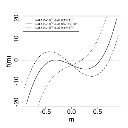
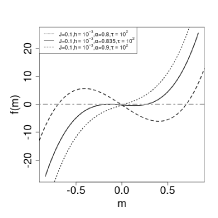
The left figure in Figure 1 shows the plot of the cubic equation (13) vs. for . , and we choose , and .
For , is the unique solution. Above , two other solutions appear: and . They are given as:
We summarize the results as:
For , becomes maximal at . For , becomes maximal at and . At , becomes minimal.
IV.2 Case
When , there is also a threshold value for . For , there is a positive real solution, , where becomes maximal. At , there are two real solutions, . The smaller solution is a multiple root of eq. (13), and is not maximal. At , becomes maximal. For , there are three real solutions: . We denote the smallest and the largest solutions as and , respectively. becomes maximal at these solutions. At the middle solution , is minimal.
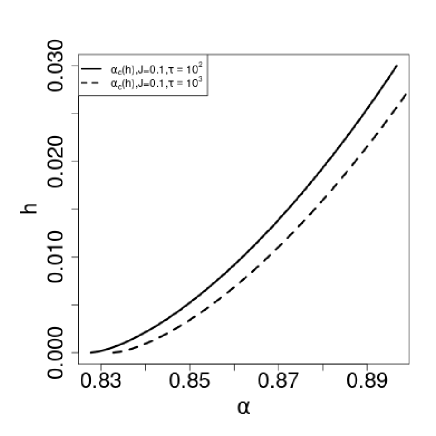
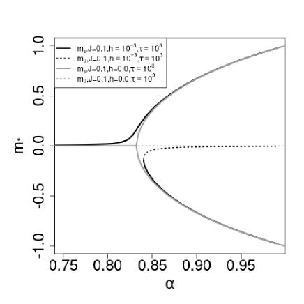
IV.3 and
We solve eq. (13) numerically to obtain . We also obtain the real solutions vs. . Figure 2 summarizes the results.
 |
 |
IV.4 Correlation of
The inverse of the covariance is given as:
The inverse matrix of , where is the identity matrix and is the matrix with all components equal to 1, is given as:
Using this result, we obtain :
The correlation coefficient between and is:
In the case , at , and . holds, and .
IV.5 Marginal pdf of
In the Gaussian approximation, for , the marginal distribution of around the mode is given as:
Here, is the unique solution of eq. (13).
For , at the critical point , diverges and the Gaussian approximation breaks down. We cannot neglect the higher order terms in , and is given as:
At the critical point , the first term on the right-hand side of becomes 1, and the second term describes the PDF.
Above , has two modes at and , where and . We denote the relative probabilities for the two modes and as and , respectively. For , . is the mixture of the two normal distributions approximately:
Here, and are estimated using and , respectively. For , we need to estimate and using the relation:
V Numerical Study of -annealing
We have conducted numerical simulations to validate the theoretical predictions associated with -annealing in the homogeneous fully connected Ising model. were sampled according to the following annealing schedule:
We set and and refer to them as ”slow” and ”fast” annealing, respectively. In the annealing process, the increment of is given by . We conducted trials for each schedule. represents the magnetization at time for during trial .
We considered a system size of spins. We set the parameters as , , and . In addition, when studying the stationary distribution of for specific , , and , we adopted the slow annealing schedule with fixed and . If reaches a specific value, we sampled only once in order to ensure the independence of the sampling process. We repeated the process times and studied the PDF of . The sample size of is .
When comparing the performance of -annealing with simulated annealing (SA), we performed SA with the conventional Metropolis-Hastings update algorithm. For , we set the final inverse temperature as and the increment of after each Monte Carlo step is set as:
We have done the sampling process times and estimated the success probability to find the ground state of the model.
The conditions for comparison of the two algorithms were kept identical. In ACO, every ant chose and the number of ants was about under the slow annealing schedule. While in SA, the final inverse temperature was reached after Monte Carlo steps (MCS). In one MCS, the number of trials for the spin update is .
V.1 Stationary distribution of
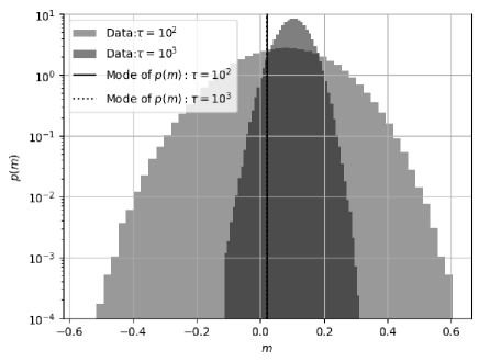
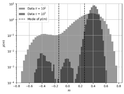
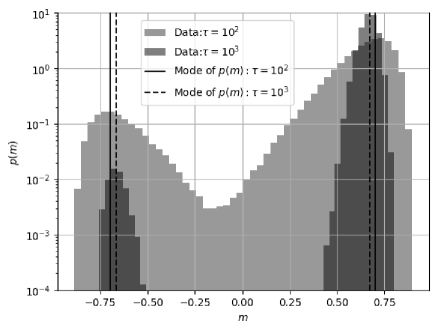
We studied the stationary distribution of . Figure 3 shows the results for the PDF of . We adopted , , and and . There are three figures for , , and , respectively. The fourth figure shows the plot of the cubic equation (13) versus for , , and . for and we chose , , and .
 |
 |
 |
 |
As one can see clearly, for , there is a unique mode for . The variance of the PDF is smaller for larger . The vertical broken line shows the position of the mode in the theory, where a discrepancy is observed. For , there are two modes and the values of the modes are almost consistent with the theoretical ones. At , for , the PDF has two modes, which is consistent with the plot of the cubic equation in the last figure (Lower Right). The profile of the cubic equation is almost flat near . The probability current is positive for , indicating that the lower mode should disappear finally. However, the stability of the mode of at is a very subtle problem. For , the profile of the PDF is not smooth and the result suggests that the equilibration is not enough for .
V.2 The comparison of -annealing with simulated annealing
We studied the performance of -annealing in ACO. We determined from by , where is the step function, i.e., for and for . The ACO system finds the ground state of the homogeneous fully connected Ising model, , if . We counted the number of samples where holds among samples and estimated the success probability. Figure 4 plots the success probability versus . For and , there are two results for both fast and slow annealing processes, respectively.
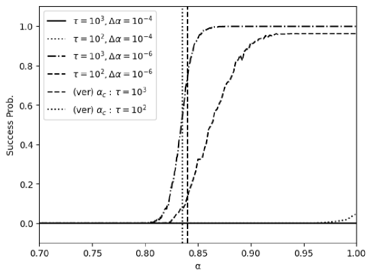
In the fast annealing cases, the success probability is almost zero and the system cannot find the ground state. In the slow annealing cases, the success probability begins to increase near . It reaches 998/1000(961/1000) at for . The success probability in SA is 0.6024 for trials. The results show that the performance of -annealed ACO is much better than that of SA.
When , the critical value of is for in SA. reaches at for . It is a rather fast annealing process and SA cannot find the ground state with high success probability. When , the correlation among the spin variables becomes strong and it becomes random whether or .
As seen in Figure 2, there is a continuous curve that connects the trivial solution for with the correct solution at . By slow annealing of , the PDF is concentrated around and the mode of is brought along the curve. When passes , the gap between and is large compared with the width of for . At , it is possible to keep the PDF around for . The system can find the ground state with high success probability. For , the width of is wide and jumps from to occur. As a result, the success probability becomes small. In fast annealing cases (), the equilibration of is not sufficient and it is difficult to align all . The success probability is much lower than the result of SA.
VI Conclusion
This paper has explored the effectiveness of -annealing within the Ant Colony Optimization (ACO) framework, particularly in seeking the ground state of the infinite-range Ising model. Our analysis, underpinned by Stochastic Differential Equations (SDEs), revealed that the joint probability density function (PDF) of the pheromone ratios is composed of two factors: entropy from the Ant System (AS) and energy from the Ising model. The parameter plays a crucial role in balancing these factors, providing a mechanism to adjust the system’s focus from broad exploratory searches to more targeted exploitative searches as increases.
We demonstrated that a smaller initially enables the system to avoid premature convergence by maintaining a broad exploration space, which is vital for escaping local minima. As increases, the exploration space narrows, allowing for intensive exploration around promising regions previously identified. This dynamic is akin to the principles observed in quantum annealing, making -annealing a potent strategy for navigating complex optimization landscapes.
Moreover, the careful management of and —particularly the rate of pheromone evaporation—is shown to be essential for the system’s ability to equilibrate and ultimately find the global minimum. Similar to temperature control in simulated annealing, and control in -annealing ensures that the system can effectively balance between exploration and exploitation, adapting to the complexity of the optimization challenges.
In conclusion, -annealing emerges as a sophisticated and efficient strategy for enhancing ACO’s performance in complex optimization scenarios. This study not only underscores the potential of -annealing as a viable alternative to traditional optimization techniques like simulated annealing but also highlights its unique ability to manage and manipulate exploration spaces dynamically. Future work will explore further applications of -annealing across different types of optimization problems, seeking to generalize these findings and refine the approach for broader practical implementation.
Acknowledgements.
This work was supported by JPSJ KAKENHI [Grant No. 22K03445].
References
- Dorigo [1992] M. Dorigo, Optimization, learning and Natural algorithms, Ph.D. thesis, Poltecnico di Milan (1992).
- Dorigo and Gambardella [1997] M. Dorigo and L. M. Gambardella, Ant colonies for the travelling salesman problem, Biosystems 43, 73 (1997).
- Deneubourg et al. [1987] J. Deneubourg, S. Aron, S. Goss, and J. Pasteels, Error, communication and learning in ant societies, European Journal of Operational Research 30, 168 (1987), modelling Complex Systems I.
- Pasteels et al. [1987] J. Pasteels, J.-L. Deneubourg, and S. Goss, Transmission and amplification of information in a changing environment: The case of insect societies, Law of Nature and Human Conduct , 129 (1987).
- Pasteels et al. [2007] J. Pasteels, J. Deneubourg, and C. Detrain, Information processing in social insects (Birkhauser Verlag, Basel, 2007).
- Camazine and Deneubourg [2001] S. Camazine and J. Deneubourg, Self-organization in biological systems (Princeton University Press, NJ, 2001).
- Kirman [1993] A. Kirman, Ants, rationality and recruitment, Q. J. Econ. 108, 137 (1993).
- Hisakado and Mori [2015] M. Hisakado and S. Mori, Information cascade, kirman’s ant colony model, and kinetic ising model, Physica A: Statistical Mechanics and its Applications 417, 63 (2015).
- Cordón et al. [2002] O. Cordón, F. Herrera, and T. Stützle, A review on the ant colony optimization metaheuristic: basis, models and new trends., Mathware and Soft Computing 9, 141 (2002).
- Dorigo and Stützle [2010] M. Dorigo and T. Stützle, Ant colony optimization: Overview and recent advances, in Handbook of Metaheuristics, edited by M. Gendreau and J.-Y. Potvin (Springer US, Boston, MA, 2010) pp. 227–263.
- Li et al. [2022] W. Li, L. Xia, Y. Huang, and S. Mahmoodi, An ant colony optimization algorithm with adaptive greedy strategy to optimize path problems, Journal of Ambient Intelligence and Humanized Computing 13, 1557 (2022).
- Tang et al. [2023] K. Tang, X.-F. Wei, Y.-H. Jiang, Z.-W. Chen, and L. Yang, An adaptive ant colony optimization for solving large-scale traveling salesman problem, Mathematics 11, 10.3390/math11214439 (2023).
- Meuleau and Dorigo [2002] N. Meuleau and M. Dorigo, Ant Colony Optimization and Stochastic Gradient Descent, Artificial Life 8, 103 (2002).
- Stutzle and Dorigo [2002] T. Stutzle and M. Dorigo, A short convergence proof for a class of ant colony optimization algorithms, IEEE Transactions on Evolutionary Computation 6, 358 (2002).
- Gutjahr [2002] W. J. Gutjahr, Aco algorithms with guaranteed convergence to the optimal solution, Information Processing Letters 82, 145 (2002).
- Gutjahr [2003] W. J. Gutjahr, A converging aco algorithm for stochastic combinatorial optimization, in Stochastic Algorithms: Foundations and Applications, edited by A. Albrecht and K. Steinhöfel (Springer Berlin Heidelberg, Berlin, Heidelberg, 2003) pp. 10–25.
- Nakamichi and Arita [2004] Y. Nakamichi and T. Arita, Diversity control in ant colony optimization, Artificial Life and Robotics 7, 198 (2004).
- Randall and Tonkes [2002] M. Randall and E. Tonkes, Intensification and diversification strategies in ant colony system, Complexity International 9, 1 (2002).
- Meyer [2008a] B. Meyer, On the convergence behaviour of ant colony search, Complexity International 12, 1 (2008a).
- Meyer [2004] B. Meyer, On the convergence behaviour of ant colony search, in Proceedings of the 7th Asia-Pacific Complex Systems Conference (COMPLEX 2004), edited by R.Stonier, Q.Han, and W.Li (Central Queensland University, Australia, 2004) pp. 153 – 167, asia-Pacific Complex Systems Conference (COMPLEX) ; Conference date: 01-01-2004.
- Meyer [2008b] B. Meyer, A tale of two wells: Noise-induced adaptiveness in self-organized systems, in 2008 Second IEEE International Conference on Self-Adaptive and Self-Organizing Systems (SASO) (IEEE Computer Society, Los Alamitos, CA, USA, 2008) pp. 435–444.
- Meyer [2017] B. Meyer, Optimal information transfer and stochastic resonance in collective decision making, Swarm Intelligence 11, 131 (2017).
- Meyer et al. [2017] B. Meyer, A. Cedrick, and T. Nakagaki, The role of noise in self-organized decision making by the true slime mold physarum polycephalum, PLOS ONE 12, 1 (2017).
- Kadowaki and Nishimori [1998] T. Kadowaki and H. Nishimori, Quantum annealing in the transverse ising model, Phys. Rev. E 58, 5355 (1998).
- Stanley [1987] H. Stanley, Introduction to Phase Transitions and Critical Phenomena, International series of monographs on physics (Oxford University Press, 1987).
- Mori et al. [2024] S. Mori, S. Nakamura, K. Nakayama, and M. Hisakado, Phase transition in ant colony optimization, Physics 6, 123 (2024).
- Gardiner [2009] C. Gardiner, Stochastic Methods: A handbook for the Natural and Social Science, 4th ed. (Springer, Berlin, 2009).
- Thouless et al. [1977] D. J. Thouless, P. W. Anderson, and R. G. Palmer, Solution of ’solvable model of a spin glass’, The Philosophical Magazine: A Journal of Theoretical Experimental and Applied Physics 35, 593 (1977), https://doi.org/10.1080/14786437708235992 .